Dynamics of a Class of Extended Duffing–Van Der Pol Oscillators: Melnikov’s Approach, Simulations, Control over Oscillations

Abstract

The Duffing–van der Pol oscillator is a very prominent and interesting standard model. There is a substantial body of varied literature on this topic. In this article, we propose a new class of oscillators by adding new factors to its dynamics. Investigations in light of Melnikov’s approach are considered. Several simulations are composed. A few specialized modules for testing the dynamics of the hypothetical oscillator under consideration are also given. This will be an essential component of a much broader Web-based scientific computing application that is planned. Possible control over oscillations: approximation with restrictions is also discussed; some probabilistic constructions are also presented.

1. Introduction

The non-autonomous Duffing–van der Pol oscillator is a very prominent and interesting standard model. The literature devoted to this issue is significant in volume and diversity.

The investigations of chemical oscillating reactions in a continuously stirred tank reactor (CSTR) [1,2,3,4,5,6,7,8] have revealed non-equilibrium phenomena such as oscillations, bi-stability, complex oscillations, and quasi-chaotic behavior of the reaction. A detailed study of a nonlinear Duffing-type oscillator driven by two voltage sources can be found in [9]. For some stochastic Duffing equations, see [10,11,12,13,14,15].

Modeling nonlinear dissipative chemical dynamics by a forced modified van der Pol–Duffing oscillator with asymmetric potential is considered in [16]

$$\left\{\begin{array}{ccc}{\displaystyle \frac{\mathrm{d}x}{\mathrm{d}t}}\hfill & =& y\hfill \\ {\displaystyle \frac{\mathrm{d}y}{\mathrm{d}t}}\hfill & =& -\alpha x-\gamma x^3-\beta +ϵ\left(-\mu (1-x^2)y+Ecos\left(\omega t\right)\right),\hfill \end{array}\right.$$

(1)

where $ϵ$ is a tiny parameter that describes how small the forced and dissipative terms are. Some additional related studies are [17,18,19,20,21].

Chaos in a nonlinear dissipative chemical oscillator, coexisting attractors, and chaos control are considered in [22] (also see [23]).

To be more specific, the authors take the model into the following [22]:

$$\left\{\begin{array}{ccc}{\displaystyle \frac{\mathrm{d}x}{\mathrm{d}t}}\hfill & =& y\hfill \\ {\displaystyle \frac{\mathrm{d}y}{\mathrm{d}t}}\hfill & =& -\alpha x-\gamma x^3-\beta +ϵ\left(-\mu (1-x^2-k_{1}xy-k_2{y}^2)y+fcos\left(\omega t\right)\right).\hfill \end{array}\right.$$

(2)

Simulations and oscillation control of a type of chemical oscillator with asymmetry potential are considered in [24]. More precisely, the next new classes of altered oscillators are presented:

$$\left\{\begin{array}{ccc}{\displaystyle \frac{\mathrm{d}x}{\mathrm{d}t}}\hfill & =& y\hfill \\ {\displaystyle \frac{\mathrm{d}y}{\mathrm{d}t}}\hfill & =& -\alpha x-\gamma x^3-\beta +ϵ\left(-\mu y+{\displaystyle \sum _{j=1}^N}{g}_{j}cos\left(j\omega t\right)\right),\hfill \end{array}\right.$$

(3)

where $0\le ϵ<1$, $\mu >0$, $g_i\ge 0,i=1,2,\dots ,N$, and N is an integer.

$$\left\{\begin{array}{ccc}{\displaystyle \frac{\mathrm{d}x}{\mathrm{d}t}}\hfill & =& y\hfill \\ {\displaystyle \frac{\mathrm{d}y}{\mathrm{d}t}}\hfill & =& -\alpha x-\gamma x^3-\beta +ϵ\left(-{\mu y\left|y\right|}^{p-1}+{\displaystyle \sum _{j=1}^N}{g}_{j}cos\left(j\omega t\right)\right),\hfill \end{array}\right.$$

(4)

where $0\le ϵ<1$, $\mu >0$, $g_i\ge 0,i=1,2,\dots ,N$, N is an integer, and p is the damping exponent.

In [25], By adding a nonlinear quintic term, the authors take into account an extended Duffing–van der Pol oscillator. The system’s dynamical behavior

$$\left\{\begin{array}{ccc}{\displaystyle \frac{\mathrm{d}x}{\mathrm{d}t}}\hfill & =& y\hfill \\ {\displaystyle \frac{\mathrm{d}y}{\mathrm{d}t}}\hfill & =& -ax-b{x}^3-c{x}^5+ϵ\left(\mu (1-x^2)y+fcos\left(\omega t\right)\right)\hfill \end{array}\right.$$

(5)

is examined by numerical simulations and Melnikov analysis. Understanding the nature of a particular nonlinear system can be aided by the findings.

Refs. [26,27] contain an analysis of the robustness and mechanism for managing chaos using a random phase. The study of parallelism in random dynamical systems and its impact on system behavior are the main topics of the paper [28]. Numerous academics have thoroughly examined this idea for deterministic dynamical systems. In the cited article, the reader can find additional references. For other results, see [29,30,31,32,33,34,35,36].

Ref. [37] examines the analysis of chaotic behavior in the extended Duffing–van der Pol system under additive non-symmetry biharmonical excitation. More precisely, the following differential model is considered:

$$\left\{\begin{array}{ccc}{\displaystyle \frac{\mathrm{d}x}{\mathrm{d}t}}\hfill & =& y\hfill \\ {\displaystyle \frac{\mathrm{d}y}{\mathrm{d}t}}\hfill & =& -c_{1}x-c_2{x}^3-c_3{x}^5-a(b_1-b_2{x}^2)y+fcos(\mathrm{\Omega }t+\mathrm{\Psi })+\hfill \\ \hfill & & +gsin(\omega t+\sigma \xi (t\left)\right),\hfill \end{array}\right.$$

(6)

where $\sigma$ is the intensity of the typical Winner process and $\xi \left(t\right)$ is the process itself.

The study of fifth-order non-smooth modified Duffing–van der Pol oscillators’ chaotic dynamics is important for upcoming studies in contemporary engineering applications.

The homoclinic and heteroclinic bifurcations in the nonlinear dynamics of models (5) and (6) can be considered in the light of the methodology proposed in the excellent article by Lenci, Menditto, and Tarantino [38].

In the cited article, the reader can find additional references on the topic under discussion.

In [39], the chaotic dynamics of an extended Duffing–van der Pol system of the following sort is examined by the authors:

$$\left\{\begin{array}{ccc}{\displaystyle \frac{\mathrm{d}x}{\mathrm{d}t}}\hfill & =& y\hfill \\ {\displaystyle \frac{\mathrm{d}y}{\mathrm{d}t}}\hfill & =& -ax-b{x}^3-c{x}^5+ϵ\left(\mu (1-x^2)y+fxcos\left(\omega t\right)-dg\left(x\right)\right),\hfill \end{array}\right.$$

(7)

where $a>0,b<0,c>0$ and the excitation amplitude, damping coefficient, excitation frequency, and disturbance amplitude are $f>0,\mu >0,\omega >0,d>0$, respectively.

In (7), $g\left(x\right)$ is considered as a periodic function of x that is not smooth with period $2l$.

Specifically, the differential model that follows has been suggested [39]:

$$\left\{\begin{array}{ccc}{\displaystyle \frac{\mathrm{d}x}{\mathrm{d}t}}\hfill & =& y\hfill \\ {\displaystyle \frac{\mathrm{d}y}{\mathrm{d}t}}\hfill & =& -ax-b{x}^3-c{x}^5+ϵ\left(\mu (1-x^2)y+fxcos\left(\omega t\right)\right.\hfill \\ \hfill & & \left.{\displaystyle -\frac{2d}{\pi }\left({\displaystyle 1-2{\displaystyle \sum _{k=1}^{\infty }}\frac{cos\left(2kx\right)}{4k^2-1}}\right)}\right).\hfill \end{array}\right.$$

(8)

We intend to add new components to the dynamics of this differential system in order to broaden its theoretical foundation. Studies are examined in the context of Melnikov’s methodology [40]. A number of simulations are created. Possible control over oscillations: approximation with restrictions is also discussed. Additionally, we present a few specific modules for examining the dynamics of the hypothetical oscillator under consideration. The obtained results can be included into a much broader scientific computing application; see [41] for additional information.

2. The New Model

We examine a novel class of hypothetical oscillators of the following kind:

$$\left\{\begin{array}{ccc}{\displaystyle \frac{\mathrm{d}x}{\mathrm{d}t}}\hfill & =& y\hfill \\ {\displaystyle \frac{\mathrm{d}y}{\mathrm{d}t}}\hfill & =& -ax-b{x}^3-c{x}^5+ϵ(\mu (1-x^2-m_{1}xy-k_1{y}^2)y+\hfill \\ \hfill & & +x{\displaystyle \sum _{i=1}^N}{g}_{i}cos\left(i\omega t\right)),\hfill \end{array}\right.$$

(9)

where $a>0$, $b<0$, $0\le ϵ<1$, $\mu >0$, $m_1>0$, $k_1>0$, $\omega >0$, $g_i\ge 0,i=1,2,\dots ,N$ (N is an integer), and c is chosen such that $b^2-4ac>0$.

We will note that the physical significance of the above-mentioned restrictive condition in terms of the coefficients of the unperturbed oscillator indicates the periodicity of the unperturbed differential system.

Let

$$\left\{\begin{array}{ccc}{\displaystyle \frac{\mathrm{d}x}{\mathrm{d}t}}\hfill & =& f_1(x,y)+ϵg_1(x,y,t)\hfill \\ {\displaystyle \frac{\mathrm{d}y}{\mathrm{d}t}}\hfill & =& f_2(x,y)+ϵg_2(x,y,t)\hfill \end{array}\right.$$

and ${\mathrm{\Gamma }}_0\left(t\right)=(x_0\left(t\right),y_0\left(t\right))$ be one of the homoclinic orbits. The Melnikov function corresponding to the system is of the form

$$M\left(t_0\right)={\displaystyle {\int }_{-\infty }^{\infty }}{e}^{-\int \nabla .f\left({\mathrm{\Gamma }}_0\left(s\right)\right)\mathrm{d}s}.f({\mathrm{\Gamma }}_0\left(t\right)\wedge g({\mathrm{\Gamma }}_0\left(t\right),t+t_0)\mathrm{d}t.$$

Considerations in the Light of Melnikov’s Approach

There are five equilibrium points for the model (9), defined as $(0,0);(\pm x_1,0);(\pm x_2,0)$, where

$$x_1=\sqrt{{\displaystyle \frac{-b-\sqrt{\mathrm{\Delta }}}{2c}}},x_2=\sqrt{{\displaystyle \frac{-b+\sqrt{\mathrm{\Delta }}}{2c}}},\mathrm{\Delta }=b^2-4ac>0.$$

The homoclinic and heteroclinic orbits connecting saddles $(\pm x_1,0)$ are as follows (see for example [38,39]):

$$\left\{\begin{array}{c}{x}_{0,\pm }\left(t\right)=\pm {\displaystyle \frac{\sqrt{2}{x}_{1}cosh\left(\frac{\gamma }{2}t\right)}{\sqrt{\beta +cosh\left(\gamma t\right)}}}\hfill \\ y_{0,\pm }\left(t\right)=\pm {\displaystyle \frac{\sqrt{2}{x}_1(\beta -1)\gamma sinh\left(\frac{\gamma }{2}t\right)}{2{(\beta +cosh\left(\gamma t\right))}^{\frac{3}{2}}}},\hfill \end{array}\right.$$

$$\left\{\begin{array}{c}{x}_{1,\pm }\left(t\right)=\pm {\displaystyle \frac{\sqrt{2}{x}_{1}sinh\left(\frac{\gamma }{2}t\right)}{{(-\beta +cosh\left(\gamma t\right))}^{\frac{1}{2}}}}\hfill \\ y_{1,\pm }\left(t\right)=\pm {\displaystyle \frac{\sqrt{2}{x}_1(1-\beta )\gamma cosh\left(\frac{\gamma }{2}t\right)}{2{(-\beta +cosh\left(\gamma t\right))}^{\frac{3}{2}}}},\hfill \end{array}\right.$$

where

$$\gamma =x_1^2\sqrt{2c({\theta }^2-1)};\beta ={\displaystyle \frac{5-3{\theta }^2}{3{\theta }^2-1}};\theta ={\displaystyle \frac{x_2}{x_1}}.$$

The homoclinic orbit for $a=0.2;b=-0.5;c=0.1$ is depicted in Figure 1.

When $ϵ\ne 0$, the Melnikov function provides a measure of the leading order distance between the stable and unstable manifolds, which may be used to determine the transverse intersection of the stable and unstable manifolds.

The integral of Melnikov by definition along the homoclinic orbit corresponding to the new model (9) is given by

$$\begin{array}{ccc}{M}_{0,\pm }\left(t_0\right)\hfill & =& {\displaystyle {\int }_{-\infty }^{\infty }}{y}_{0,\pm }\left(t\right)(\mu y_{0,\pm }\left(t\right)-\mu x_{0,\pm }^2\left(t\right)y_{0,\pm }\left(t\right)-\mu m_1{x}_{0,\pm }\left(t\right)y_{0,\pm }^2\left(t\right)-\hfill \\ \hfill & & \mu k_1{y}_{0,\pm }^3\left(t\right)+x_{0,\pm }\left(t\right){\displaystyle \sum _{i=1}^N}{g}_{i}cos\left(i\omega (t+t_0)\right))\mathrm{d}t.\hfill \end{array}$$

(10)

The task of determining the root of $M_{0,\pm }\left(t_0\right)$ is more intriguing from a numerical perspective because the parameters that appear in the suggested differential model are subject to several practical and physical constraints.

It is known that if $M_{0,\pm }\left(t_0\right)=0$ and ${\displaystyle \frac{\mathrm{d}{M}_{0,\pm }\left(t_0\right)}{\mathrm{d}{t}_0}}\ne 0$ for some $t_0$ and some sets of parameters (transversal junction conditions), then a homoclinic bifurcation takes place, indicating the potential for chaotic behavior.

For the Melnikov function $M_{0,\pm }\left(t_0\right)$, in the specific situation $N=1$, we have

$$M_{0,\pm }\left(t_0\right)=\mu \left(I_1-I_2-m_1{I}_3-k_1{I}_4\right)-g_{1}sin\left(\omega t_0\right)I_5,$$

(11)

where

$$I_1={\displaystyle {\int }_{-\infty }^{\infty }}{y}_{0,\pm }^2\left(t\right)\mathrm{d}t,$$

$$I_2={\displaystyle {\int }_{-\infty }^{\infty }}{x}_{0,\pm }^2\left(t\right)y_{0,\pm }^2\left(t\right)\mathrm{d}t,$$

$$I_3={\displaystyle {\int }_{-\infty }^{\infty }}{x}_{0,\pm }\left(t\right)y_{0,\pm }^3\left(t\right)\mathrm{d}t,$$

$$I_4={\displaystyle {\int }_{-\infty }^{\infty }}{y}_{0,\pm }^4\left(t\right)\mathrm{d}t,$$

$$I_5={\displaystyle {\int }_{-\infty }^{\infty }}{x}_{0,\pm }\left(t\right)y_{0,\pm }\left(t\right)sin\left(\omega t\right)\mathrm{d}t.$$

Proposition 1. 

If $N=1$, then the roots of the Melnikov function $M_{0,\pm }\left(t_0\right)$ are given as solutions of the equation $M_{0,\pm }\left(t_0\right)=0$ (see Figure 2).

Remark 1. 

In formulating and proving Proposition 1, we used a significantly specialized module for investigating the dynamics of the considered hypothetical oscillator, implemented in the computer algebraic system for scientific calculations—CAS Mathematica.

Remark 2. 

From Proposition 1, we obtain the condition that the Melnikov function $M_{0,\pm }\left(t_0\right)$ has simple zeros and chaos occurs as follows:

$$\left|{\displaystyle \frac{\mu (I_1-I_2-m_1{I}_3-k_1{I}_4)}{g_1{I}_5}}\right|<1.$$

We leave the detailed study of this criterion (as a function of the parameters of our model (9)) to the reader. Below, we will consider some typical examples.

Remark 3. 

Chaotic features on system parameters for heteroclinic orbit, and also the Melnikov functions and parameter conditions for these orbits, are investigated in a similar way and will be omitted here. It is enough for the reader to strictly follow the research plan proposed for such oscillators in the excellent article in [39].

Example 1. 

For $N=1$, $a=0.37$, $b=-0.5$, $c=0.16$, $\mu =0.5$, $k_1=0.9$, $m_1=0$, $\omega =0.27$, $g_1=0.25$, the Melnikov function is depicted in Figure 3a.

Example 2. 

For $N=1$, $a=0.37$, $b=-0.5$, $c=0.16$, $\mu =0.71$, $k_1=0.06$, $m_1=0$, $\omega =0.1$, $g_1=0.1$, the Melnikov function is depicted in Figure 3b.

Some notes:

• Melnikov’s criterion for the occurrence of the intersection between the disturbed and unperturbed separatrices for a fixed N can be formulated by the reader. In this case, the explicit representation of $M_{0,\pm }\left(t_0\right)$ (moreover, for high values of the parameter N) is laborious. In order to employ specialized modules provided in current computer algebraic systems for scientific study, the user should first conduct a series of preparatory operations on the integrals $I_j$ as previously stated.
• Prior to that, while calculating the integral (8), it is convenient to adopt the following representation: $cos\left(i\omega (t+t_0)\right)=cos\left(i\omega t\right)cos\left(i\omega t_0\right)-sin\left(i\omega t\right)sin\left(i\omega t_0\right)$.

Some extended differential models are examined in the context of Melnikov’s method (see [42,43,44,45,46,47]). Refs. [48,49,50,51] contain numerical techniques for resolving nonlinear equations.

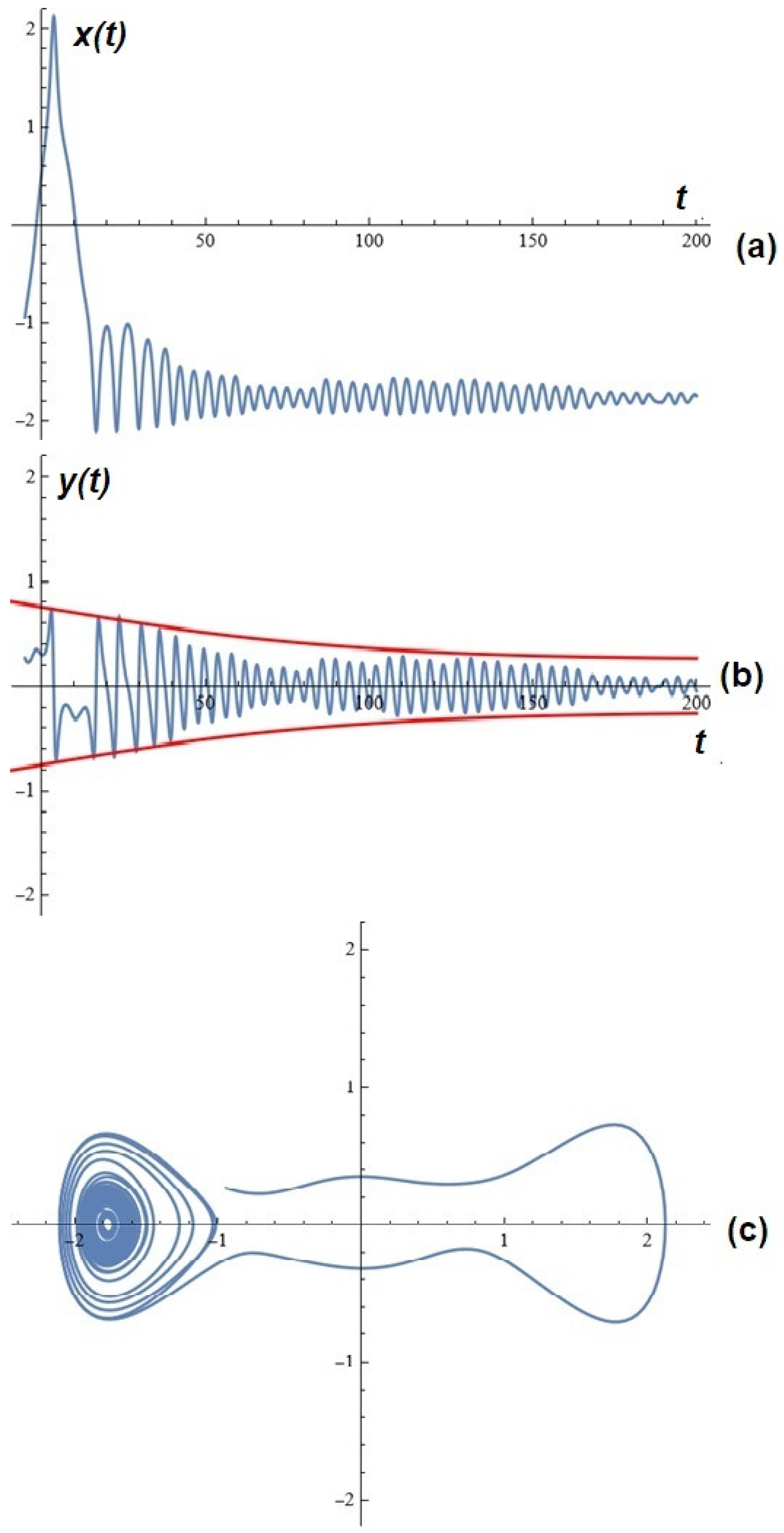
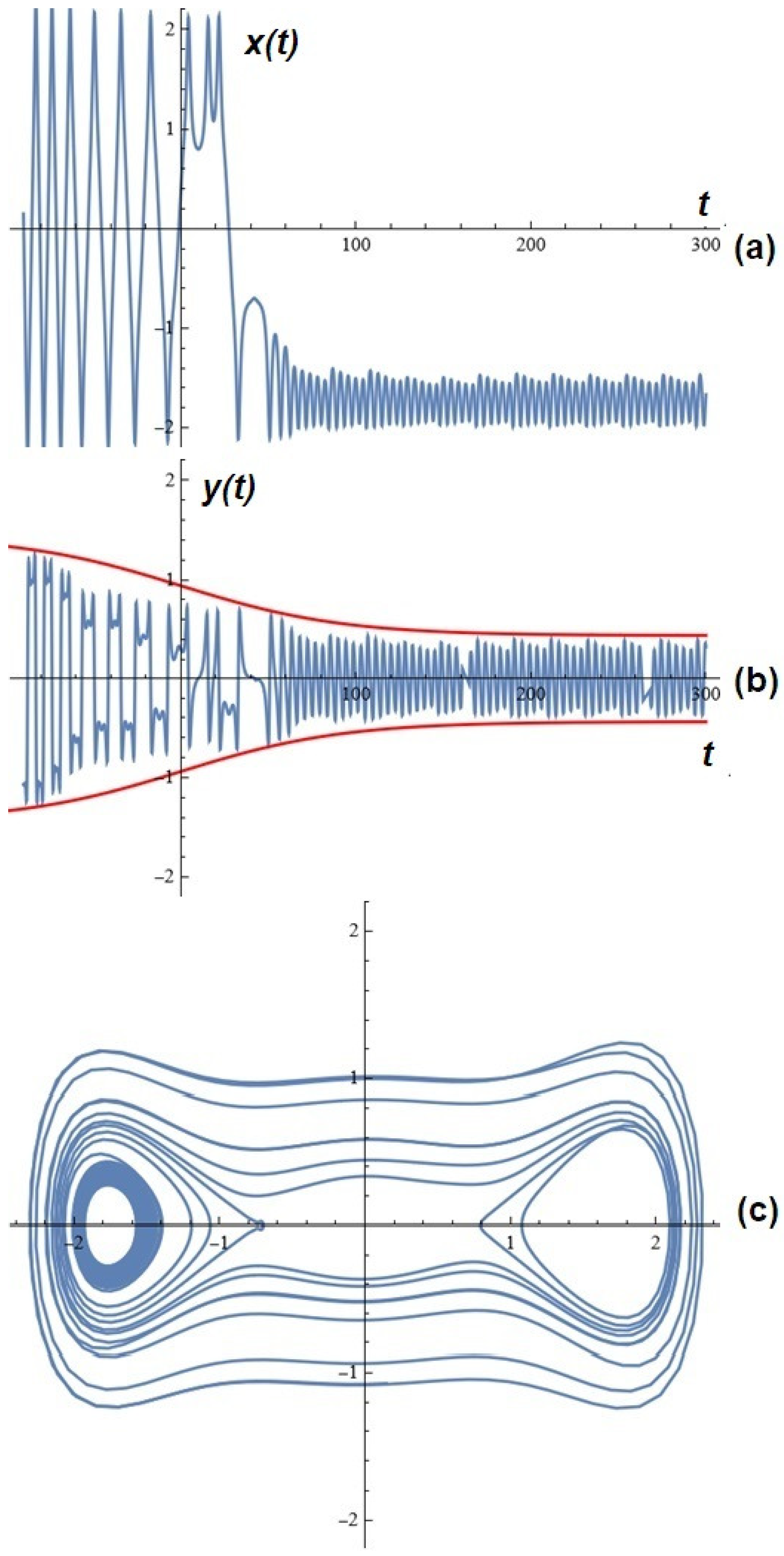
3. A Few Simulations

Here, we will focus on some interesting simulations:

Example 3. 

For given $N=4$, $a=0.2$, $b=-0.5$, $c=0.1$, $\mu =0.2$, $k_1=0.1$, $m_1=0.1$, $\omega =0.4$, $g_1=0.9$, $g_2=0.1$, $g_3=0.3$, $g_4=0.7$, and $ϵ=0.015$, the system’s simulations (9) for $x_0=0.4$ and $y_0=0.1$ are depicted in Figure 4.

Example 4. 

For given $N=6$, $a=0.25$, $b=-0.56$, $c=0.15$, $\mu =3$, $k_1=0.1$, $m_1=0.09$, $\omega =0.4$, $g_1=0.9$, $g_2=0.1$, $g_3=0.3$, $g_4=0.2$, $g_5=0.4$, and $g_6=0.8ϵ=0.015$, the system’s simulations (9) for $x_0=0.5$ and $y_0=0.3$ are depicted in Figure 5.

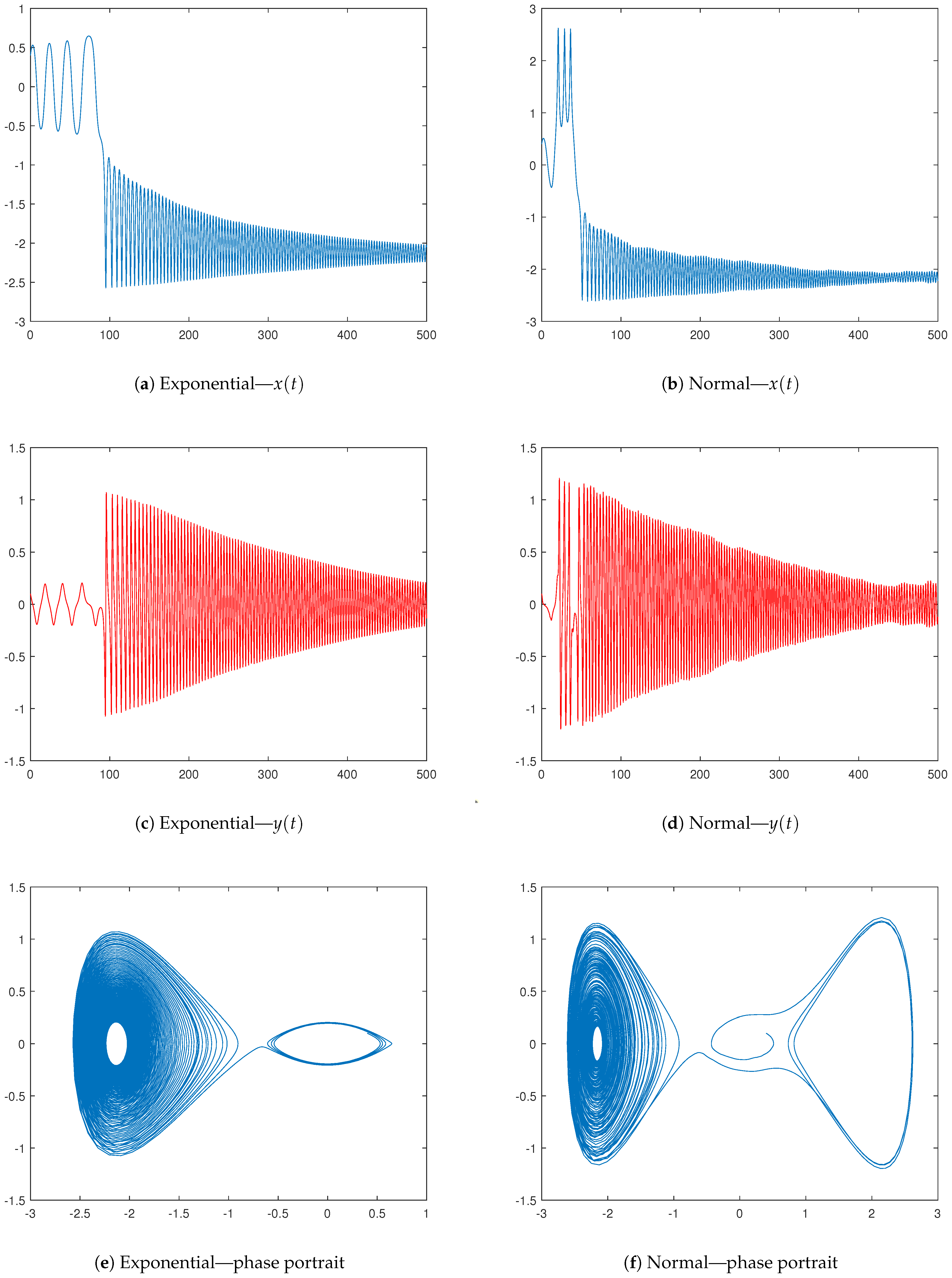
4. Potential Control over Oscillations

A user-preset level (or fork) for the oscillations of the y component of the differential system solution is one of the several free parameters that make the new model (9) appealing for engineering computations.

Assume that the fork or constraint $\left(F\right(t),-F(t\left)\right)$ is of the following type (most typical restriction):

$$F\left(t\right)=a_1+{\displaystyle \frac{a_2}{1+e^{a_{3}t}}}.$$

(12)

To be thorough, we will look at another simulation using the differential model (9) that was previously suggested.

Example 5. 

For given $N=8$, $a=0.256$, $b=-0.567$, $c=0.1545$, $\mu =1.8$, $k_1=0.12$, $m_1=0.078$, $\omega =0.3$, $g_1=0.9$, $g_2=\dots =g_7=0.851$, $g_8=0.9$, and $ϵ=0.01$, the system’s simulations (9) for $x_0=0.5$ and $y_0=0.3$ are depicted in Figure 6.

Using the exponential-type function $F\left(t\right)$ and user-fixed $N=8$

$$F\left(t\right)=-0.25-{\displaystyle \frac{1.01}{1+{\displaystyle e^{0.0211t}}}}$$

for the parameters specified in Example 5 (see Figure 6b), the desired control over oscillations is obtained.

Example 6. 

For given $N=10$, $a=0.256$, $b=-0.567$, $c=0.1545$, $\mu =1.8$, $k_1=0.12$, $m_1=0.078$, $\omega =0.3$, $g_1=0.9$, $g_2=\dots =g_7=0.85$, $g_8=0.9$, $g_9=0.4$, $g_{10}=0.1$, and $ϵ=0.01$, the system’s simulations (9) for $x_0=0.4$ and $y_0=0.3$ are depicted in Figure 7.

With $N=10$ set by the user and the function $F\left(t\right)$ of the kind

$$F\left(t\right)=-0.44-{\displaystyle \frac{0.995}{1+{\displaystyle e^{0.02181t}}}}$$

for the parameters specified in Example 6 (see Figure 7b), the desired control over oscillations is obtained.

Remark 4. 

Depending on the oscillator profile, other approximations may be used, for example, $F\left(t\right)$ may be of the exponential, log-logistic, hyper-log-logistic, piecewise smooth sigmoid, Gompertz, or activation type.

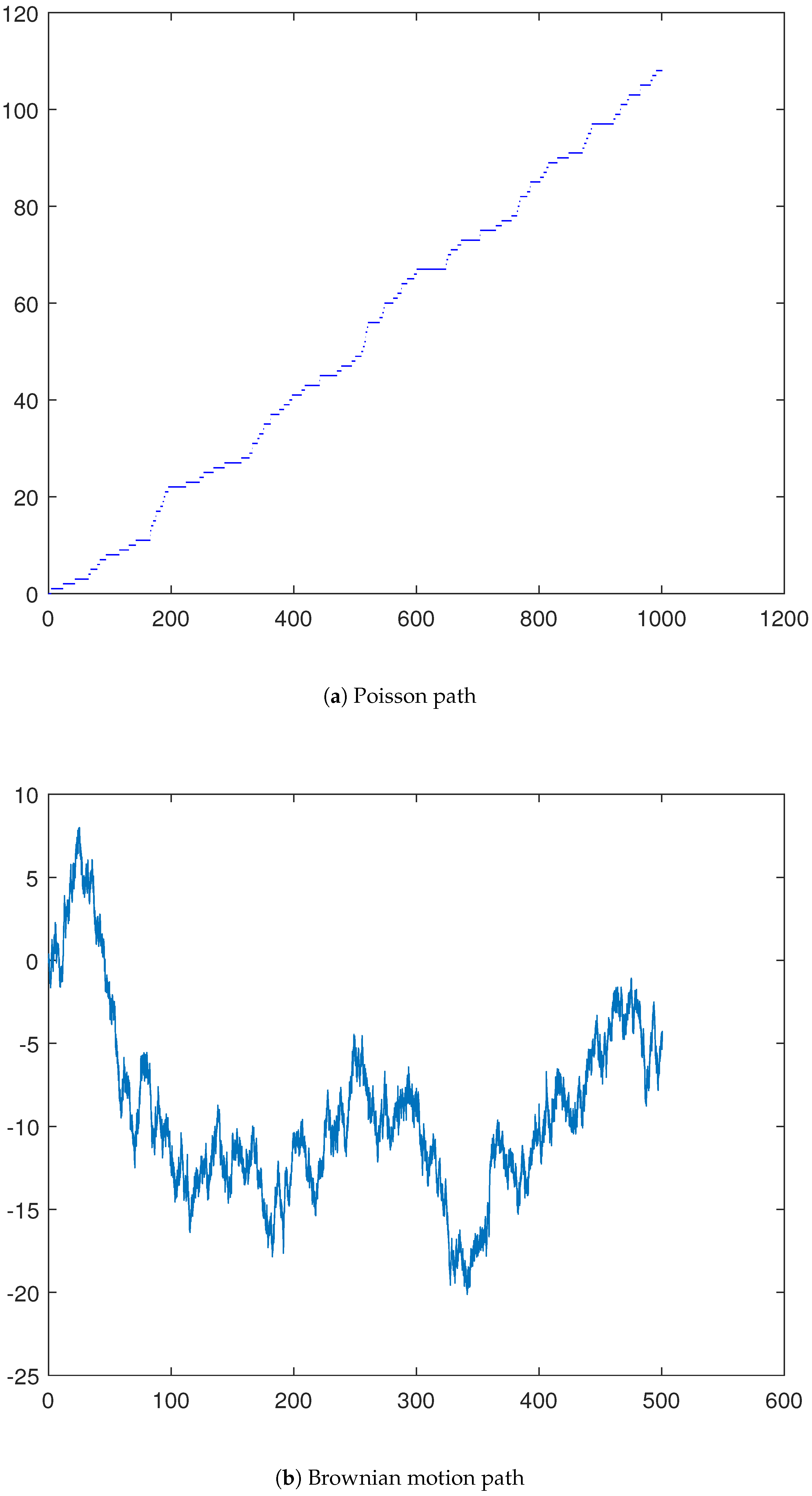
Some Probabilistic Constructions

Suppose that ${\sum }_{j=1}^N{g}_j=1$—this restriction is not essential since we may achieve it after scaling. The probabilities of a random variable $\xi$ specified on the domain $\left\{1,2,\dots ,N\right\}$ can therefore be viewed as the coefficient $g_j$. Let $\mathrm{\Psi }\left(·\right)$ be its characteristic function. Keeping in mind the exponential presentation of the cos function

$$cos\left(x\right)={\displaystyle \frac{e^{ix}+e^{-ix}}{2}},$$

(13)

we transform model (9) into

$$\begin{array}{cc}\hfill {\displaystyle \frac{\mathrm{d}y}{\mathrm{d}t}}& =-ax-b{x}^3-c{x}^5+ϵ\left(\begin{array}{c}\mu \left(1-x^2-m_{1}xy-k_1{y}^2\right)y\hfill \\ +x{\displaystyle \sum _{j=1}^N}{g}_j{\displaystyle \frac{e^{ij\omega t}+e^{-ij\omega t}}{2}}\hfill \end{array}\right)\hfill \\ \hfill & =-ax-b{x}^3-c{x}^5+ϵ\left(\begin{array}{c}\mu \left(1-x^2-m_{1}xy-k_1{y}^2\right)y\hfill \\ +x{\displaystyle \frac{\mathbb{E}\left[e^{i\omega t\xi }\right]+\mathbb{E}\left[e^{-i\omega t\xi }\right]}{2}}\hfill \end{array}\right)\hfill \\ \hfill & =-ax-b{x}^3-c{x}^5+ϵ\left(\begin{array}{c}\mu \left(1-x^2-m_{1}xy-k_1{y}^2\right)y\hfill \\ +x{\displaystyle \frac{\mathrm{\Psi }\left(\omega t\right)+\mathrm{\Psi }\left(-\omega t\right)}{2}}\hfill \end{array}\right).\hfill \end{array}$$

(14)

We can conclude that the condition $\xi$ to be distributed on the domain $\left\{1,2,\dots ,N\right\}$ is not essential. If we generalize it to the set D, then we can rewrite the dynamics (9) as

$${\displaystyle \frac{\mathrm{d}y}{\mathrm{d}t}}=-ax-b{x}^3-c{x}^5+ϵ\left(\begin{array}{c}\mu \left(1-x^2-m_{1}xy-k_1{y}^2\right)y\hfill \\ +x\underset{D}{\int }cos\left(u\omega t\right)g\left(du\right)\hfill \end{array}\right).$$

(15)

Note that the probabilities $g_j$ are generalized to the measure $g\left(du\right)$.

We prepare some simulations based on the $\left(q,\sigma \right)$-normal distribution and on the exponential one, whose intensity is denoted by $\lambda$. Their probability densities are

$$\begin{array}{cc}\hfill f_{Gaussian}\left(x\right)& ={\displaystyle \frac{1}{\sqrt{2\pi {\sigma }^2}}}{e}^{-{\displaystyle \frac{{\left(x-q\right)}^2}{2{\sigma }^2}}},\hfill \\ \hfill f_{exponential}\left(x\right)& =\lambda e^{-\lambda x}.\hfill \end{array}$$

(16)

The domains are $D=\mathbb{R}$ and $D={\mathbb{R}}^{+}$, respectively. The characteristic functions

$$\begin{array}{cc}\hfill {\mathrm{\Psi }}_{Gaussian}\left(x\right)& =e^{iqx-{\displaystyle \frac{{\sigma }^2{x}^2}{2}}},\hfill \\ \hfill {\mathrm{\Psi }}_{exponential}\left(x\right)& ={\displaystyle \frac{\lambda }{\lambda -ix}}.\hfill \end{array}$$

(17)

Keeping in mind the following relations for the characteristic functions

$$\begin{array}{cc}\hfill & {\mathrm{\Psi }}_{Gaussian}\left(x\right)+{\mathrm{\Psi }}_{Gaussian}\left(-x\right)=2e^{-{\displaystyle \frac{{\sigma }^2{x}^2}{2}}}cos\left(qx\right),\hfill \\ \hfill & {\mathrm{\Psi }}_{exponential}\left(x\right)+{\mathrm{\Psi }}_{exponential}\left(-x\right)=2{\displaystyle \frac{{\lambda }^2}{{\lambda }^2+x^2}},\hfill \end{array}$$

(18)

we transform the dynamics (14) into

$${\displaystyle \frac{\mathrm{d}y}{\mathrm{d}t}}=-ax-b{x}^3-c{x}^5+ϵ\left(\begin{array}{c}\mu \left(1-x^2-m_{1}xy-k_1{y}^2\right)y\hfill \\ +x{e}^{-{\displaystyle \frac{{\sigma }^2{\omega }^2{t}^2}{2}}}cos\left(q\omega t\right)\hfill \end{array}\right)$$

(19)

for the Gaussian simulation. Let us discuss the effect of the parameters on the model. The expectation q has a scaling role in the periodic function and thus it does not lead to a significant generalization. However, this is not the case for $\sigma$. First, for small time values, $\sigma$ has a more significant impact. When sigma is near zero, the exponent is near one and thus the model is similar to the original formulation with one periodic function. On the other hand, when $\sigma$ tends to infinity, then the exponent vanishes and thus the impact of the periodic function is negligible. The same conclusions can be deduced for the larger values of t but for closer to zero (infinity) values of $\sigma$—at larger t, extreme values of $\sigma$ are necessary to capture the desired behavior.

We have the following for the exponential distribution:

$${\displaystyle \frac{\mathrm{d}y}{\mathrm{d}t}}=-ax-b{x}^3-c{x}^5+ϵ\left(\begin{array}{c}\mu \left(1-x^2-m_{1}xy-k_1{y}^2\right)y\hfill \\ +x{\displaystyle \frac{{\lambda }^2}{{\lambda }^2+{\omega }^2{t}^2}}\hfill \end{array}\right).$$

(20)

We can see that the exponential distribution introduces a damping x-term in the model reciprocal to the square of the time. The intensity $\lambda$ can be viewed as a scaling parameter—as the larger $\lambda$ is, the larger t has to be. Furthermore, this dependence is linear. We present the x- and y-dynamics as well as the phase portraits in Figure 8. The first column is for the normal distribution ($q=1,\sigma =1$), whereas the exponential simulations with intensity $\lambda =1$ are presented in the second column. For the rest of the parameters, we chose Example 3.

5. Concluding Remarks and Further Work

In this research, we have examined a novel hypothetical differential model that has a large number of free parameters, which makes it appealing to users. To examine the behavior of these oscillators, we present a several specialized modules.

For some of them, a cloud version is available that just requires a browser and an internet connection.

This will be an essential component of a much broader Web-based program for scientific computing that is in the works.

We have tried, as far as possible, to comply with the proposed standard for the publication of new chaotic systems [52].

We envisage future research on the topic—the modeling of chaotic systems with a desired set of properties [53,54].

Last but not least, we provide some simulations based on the idea of [37] to introduce a stochastic element in the dynamical model. We suggest two methods. The first one is inspired by [37]—thus, the dynamics (14) turn into

$$\begin{array}{cc}\hfill {\displaystyle \frac{\mathrm{d}y}{\mathrm{d}t}}& =-ax-b{x}^3-c{x}^5+ϵ\left(\begin{array}{c}\mu \left(1-x^2-m_{1}xy-k_1{y}^2\right)y\hfill \\ +x{\displaystyle \frac{\mathrm{\Psi }\left(\omega t+N_t\right)+\mathrm{\Psi }\left(-\omega t-N_t\right)}{2}}\hfill \end{array}\right).\hfill \end{array}$$

(21)

We assume that $N_t$ is a homogenous Poisson process. We present in the first column of Figure 9 the related simulations when we consider the exponential modification from Section Some Probabilistic Constructions. The intensity of the Poisson process is assumed to be $\delta =10$. Alternatively, in the second column we present the results for the following dynamics:

$$\begin{array}{cc}\hfill {\displaystyle \frac{\mathrm{d}y}{\mathrm{d}t}}& =-ax-b{x}^3-c{x}^5+ϵ\left(\begin{array}{c}\mu \left(1-x^2-m_{1}xy-k_1{y}^2\right)y\hfill \\ +x{\displaystyle \frac{\mathrm{\Psi }\left(\omega t\right)+\mathrm{\Psi }\left(-\omega t\right)}{2}}+B_t\hfill \end{array}\right),\hfill \end{array}$$

(22)

where $B_t$ is a standard Brownian motion. We apply the Gaussian example from Section Some Probabilistic Constructions. The generated sample paths of the Poisson process and the Brownian motion can be viewed in Figure 10.

The analysis of models (21) and (22) is left for further work.

Analytical estimates of the effect of an amplitude-modulated (AM) signal in nonlinearly damped Duffing–van der Pol oscillators are considered in [55]. More precisely, the authors presented the following model:

$$\left\{\begin{array}{ccc}{\displaystyle \frac{\mathrm{d}x}{\mathrm{d}t}}\hfill & =& y\hfill \\ {\displaystyle \frac{\mathrm{d}y}{\mathrm{d}t}}\hfill & =& ax-b{x}^3+ϵ(-\gamma (1-x^2)y{\left|y\right|}^{p-1}+\hfill \\ & & +(f+2gcos(\mathrm{\Omega }t\left)\right)sin\left(\omega t\right)),\hfill \end{array}\right.$$

where $2g$ is the degree of modulation, and $\mathrm{\Omega }$ and $\omega$ are the frequencies of the amplitude-modulated (AM) signal.

We plan to expand the theoretical basis of this differential system in a future paper by adding new factors to its dynamics:

$$\left\{\begin{array}{ccc}{\displaystyle \frac{\mathrm{d}x}{\mathrm{d}t}}\hfill & =& y\hfill \\ {\displaystyle \frac{\mathrm{d}y}{\mathrm{d}t}}\hfill & =& -ax-b{x}^3-c{x}^5+ϵ(-\gamma (1-x^2)y{\left|y\right|}^{p-1}+\hfill \\ & & +(f+2gcos\left(\mathrm{\Omega }t\right)){\displaystyle \sum _{i=1}^N}{g}_{i}sin\left(i\omega t\right)).\hfill \end{array}\right.$$

Such an interpretation would allow for a detailed study of the dynamics of similar models at a higher energy level. The stochastic analysis of the mentioned model is also left for further work.

The reader may find other results on the topics—chaotic transitions in stochastic dynamical systems and the application of Melnikov processes in engineering, physics, and neuroscience in the book in [56].

Over the past few years, intensive work has been carried out on the important topic of estimating rate-induced tipping via asymptotic series and a Melnikov-like method.

So, for example, in [57], the authors show that a Melnikov-inspired method employing the asymptotic series allows the tipping point to be asymptotically approximated.

Investigations on bifurcation and rate-induced tipping can be found in [58]. For other basic results, see [59,60].

We envisage research in the light of the results obtained in the above-cited articles on new differential models, which are modifications of the models described in the present article.

Examples 5 and 6 considered in Section 4 are study examples. The real task that we set for the students is as follows: For fixed N, $ϵ$, and $x_0$, $y_0$, generate an appropriate simulation of model (9), if the additional user constraint is set, the oscillations on the y- component of the system solutions fall into the fork $(-F(t),F(t\left)\right)$.

After using the specialized module provided by us (with additional approximation and optimization algorithms included) implemented in CAS Mathematica, the students relatively easily arrive at the answer to the task, namely determining all the remaining parameters of the model.

Our problems to be solved are about making the use of modern GPT technologies harder (or even impossible), as they are massively used by students for the realization of their scientific tasks.

We will be glad if this article provokes an interesting discussion about the teaching methodology in this field of scientific knowledge.

References

- Boissonade, J.; De Kepper, P. Transitions from bistability to limit cycle oscillations. Theoretical analysis and experimental evidence in an open chemical system. J. Phys. Chem. 1980, 84, 501–506. [Google Scholar] [CrossRef]
- Zhabotinskii, A.M. Biological and Biochemical Oscillators; Academic Press: New York, NY, USA, 1972. [Google Scholar]
- Epstein, I.R.; Showalter, K. Nonlinear chemical dynamics: Oscillations, patterns, and chaos. J. Phys. Chem. 1996, 100, 13132–13147. [Google Scholar] [CrossRef]
- Belousov, B.P. Oscillations and Travelling Waves in Chemical Systems; Wiley: New York, NY, USA, 1985. [Google Scholar]
- Zhabotinsky, A.M.; Buchholtz, F.; Kiyatkin, A.B.; Epstein, I.R. Oscillations and waves in metal-ion-catalyzed bromate oscillating reactions in highly oxidized states. J. Phys. Chem. 1993, 97, 7578–7584. [Google Scholar] [CrossRef]
- Zhang, D.; Gyorgyi, L.; Peltier, W.R. Deterministic chaos in the Belousov-Zhabotinsky reaction: Experiments and simulations. Chaos 1993, 3, 723–745. [Google Scholar] [CrossRef]
- Ali, F.; Menzinger, M. Stirring effects and phase-dependent inhomogeneity in chemical oscillations: The Belousov-Zhabotinsky reaction in a CSTR. J. Phys. Chem. A 1997, 101, 2304–2309. [Google Scholar] [CrossRef]
- Bartuccelli, M.; Gentile, G.; Wright, J.A. Stable dynamics in forced systems with sufficiently high/low forcing frequency. Chaos 2016, 26, 083108. [Google Scholar] [CrossRef]
- Maaita, J.O.; Kyprianidis, I.M.; Volos, C.K.; Meletlidou, E. The study of a nonlinear duffing–type oscillator driven by two voltage sources. J. Eng. Sci. Technol. Rev. 2013, 6, 74–80. [Google Scholar] [CrossRef]
- Ott, E.; Grebogi, C.; Yorke, J.A. Controlling chaos. Phys. Rev. Lett. 1990, 64, 1196. [Google Scholar] [CrossRef]
- Ariaratnam, S.T.; Xie, W.C. Almost-sure stochastic stability of coupled non-linear oscillators. Int. J. Non-Linear Mech. 1994, 29, 197–204. [Google Scholar] [CrossRef]
- Kloeden, P.E.; Platen, E. Numerical Solution of Stochastic Differential Equations; Springer: Berlin/Heidelberg, Germany, 1992. [Google Scholar]
- Lin, H.; Yim, S.C.S. Analysis of a nonlinear system exhibiting chaotic, noisy chaotic and random behaviors. J. Appl. Mech. 1996, 63, 509–516. [Google Scholar] [CrossRef]
- Liu, W.Y.; Zhu, W.Q.; Huang, Z.L. Effect of bounded noise on chaotic motion of duffing oscillator under parametric excitation. Chaos Solitons Fractals 2001, 12, 527–537. [Google Scholar] [CrossRef]
- Lin, Y.K.; Cai, G.Q. Probabilistic Structural Dynamics: Advanced Theory and Applications; McGraw-Hill College: New York, NY, USA, 1995. [Google Scholar]
- Miwadinou, C.H.; Monwanou, A.V.; Yovogan, J.; Hinvi, L.A.; Tuwa, P.N.; Orou, J.C. Modeling nonlinear dissipative chemical dynamics by a forced modified Van der Pol-Duffing oscillator with asymmetric potential: Chaotic behaviors predictions. Chin. J. Phys. 2018, 56, 1089–1104. [Google Scholar] [CrossRef]
- Miwadinou, C.H.; Monwanou, A.V.; Hinvi, L.A.; Koukpemedji, A.A.; Ainamon, C.; Chabi Orou, J.B. Melnikov chaos in a modified Rayleigh-Duffing oscillator with ϕ6 potential. Int. J. Bifurc. Chaos 2016, 26, 1650085. [Google Scholar] [CrossRef]
- Ainamon, C.; Miwadinou, C.H.; Monwanou, A.V.; Orou, J.C. Analysis of multiresonance and chaotic behavior of the polarization in materials modeled by a duffing equation with multifrequency excitations. Appl. Phys. Res. 2014, 6, 74–86. [Google Scholar] [CrossRef]
- Miwadinou, C.H.; Monwanou, A.V.; Orou, J.B. Active control of the parametric resonance in the modified Rayleigh-Duffing oscillator. Afr. Rev. Phys. 2014, 9, 227–235. [Google Scholar]
- Miwadinou, C.H.; Monwanou, A.V.; Orou, J.B. Effect of nonlinear dissipation on the basin boundaries of a driven two-well modified Rayleigh-Duffing oscillator. Int. J. Bifurc. Chaos 2015, 25, 1550024. [Google Scholar] [CrossRef]
- Miwadinou, C.H.; Hinvi, A.L.; Monwanou, A.V.; Orou, J.B. Nonlinear dynamics of a ϕ6 modified duffing oscillator: Resonant oscillations and transition to chaos. Nonlinear Dyn. 2017, 88, 97–113. [Google Scholar] [CrossRef]
- Adéchinan, A.J.; Kpomahou, Y.J.F.; Hinvi, L.A.; Miwadinou, C.H. Chaos, coexisting attractors and chaos control in a nonlinear dissipative chemical oscillator. Chin. J. Phys. 2022, 77, 2694–2697. [Google Scholar] [CrossRef]
- Adéchinan, J.A.; Kpomahou, Y.J.F.; Miwadinou, C.H.; Hinvi, L.A. Dynamics and active control of chemical oscillations modeled as a forced generalized Rayleigh oscillator with asymmetric potential. Int. J. Basic Appl. Sci. 2021, 10, 20–31. [Google Scholar]
- Kyurkchiev, N.; Zaevski, T.; Iliev, A.; Kyurkchiev, V.; Rahnev, A. Dynamics of a class of chemical oscillators with asymmetry potential: Simulations and control over oscillations. Mathematics 2025, 13, 1129. [Google Scholar] [CrossRef]
- Yu, J.; Li, J. Investigation on dynamics of the extended Duffing-Van der Pol system. Z. Naturforsch. A 2009, 64, 341–346. [Google Scholar] [CrossRef]
- Lei, Y.; Xu, W.; Xu, Y.; Fang, T. Chaos control by harmonic excitation with proper random phase. Chaos Solitons Fractals 2004, 21, 1175–1181. [Google Scholar] [CrossRef]
- Xu, Y.; Mahmoud, G.M.; Xu, W.; Lei, Y. Suppressing chaos of a complex Duffing’s system using a random phase. Chaos Solitons Fractals 2005, 23, 265–273. [Google Scholar] [CrossRef]
- Kadhim, I.J.; Yasir, A.A. Lyapunov stability, parallelizablity, and symmetry of random dynamical systems. Symmetry 2025, 17, 325. [Google Scholar] [CrossRef]
- Arnold, L.; Schmalfuss, B. Lyapunov’s second method for random dynamical systems. J. Differ. Eq. 2001, 177, 235–265. [Google Scholar] [CrossRef]
- Lukashiv, T.; Litvinchuk, Y.; Malyk, I.V.; Golebiewska, A.; Nazarov, P.V. Stabilization of stochastic dynamical systems of a random structure with Markov switches and Poisson perturbations. Mathematics 2023, 11, 582. [Google Scholar] [CrossRef]
- Chueshov, I. Monotone Random Systems Theory and Applications; Springer: Heidelberg, Germany, 2002. [Google Scholar]
- Molchanov, I. Theory of Random Sets; Springer: London, UK, 2005. [Google Scholar]
- Alkhrayfawee, N.G.; Kadhim, I.J.; Albukhuttar, A.N. P- Omega limit set in random dynamical systems. J. Phys. Conf. Ser. 2022, 2322, 012041. [Google Scholar] [CrossRef]
- Wei, J.G.; Leng, G. Lyapunov exponent and chaos of Duffing’s equation perturbed by white noise. Appl. Math. Comput. 1997, 88, 77–93. [Google Scholar] [CrossRef]
- Kumar, P.; Narayanan, S.; Gupta, S. Stochastic bifurcations in a vibro-impact Duffing–Van der Pol oscillator. Nonlinear Dyn. 2016, 85, 439–452. [Google Scholar] [CrossRef]
- Abdullah, N.; Kadhim, I.J.; Kadhim, A.N. Attraction properties and asymptotically equivalent of random dynamical system. Int. J. Mech. Eng. 2022, 7, 3674–3680. [Google Scholar]
- Li, Z.G.; Xu, W.; Zhang, X.Y. Analysis of chaotic behavior in the extended duffing–van der Pol system subject to additive non-symmetry biharmonical excitation. Appl. Math. Comput. 2006, 183, 858–871. [Google Scholar] [CrossRef]
- Lenci, S.; Menditto, G.; Tarantino, A.M. Homoclinic and heteroclinic bifurcations in the non-linear dynamics of a beam resting on an elastic substrate. Int. J. Non-Linear Mech. 1999, 34, 615–632. [Google Scholar] [CrossRef]
- Hu, S.; Zhou, L. Chaotic dynamics of an extended Duffing-van der Pol system with a non-smooth perturbation and parametric excitation. Z. Naturforsch. A 2023, 78, 1015–1030. [Google Scholar] [CrossRef]
- Melnikov, V.K. On the stability of a center for time–periodic perturbation. Trans. Mosc. Math. Soc. 1963, 12, 3–52. [Google Scholar]
- Golev, A.; Terzieva, T.; Iliev, A.; Rahnev, A.; Kyurkchiev, N. Simulation on a generalized oscillator model: Web-based application. C. R. L’Acad. Bulg. Sci. 2024, 77, 230–237. [Google Scholar] [CrossRef]
- Kyurkchiev, N.; Zaevski, T.; Iliev, A.; Kyurkchiev, V.; Rahnev, A. Modeling of some classes of extended oscillators: Simulations, algorithms, generating chaos, and open problems. Algorithms 2024, 17, 121. [Google Scholar] [CrossRef]
- Kyurkchiev, N.; Zaevski, T.; Iliev, A.; Kyurkchiev, V.; Rahnev, A. Generating chaos in dynamical systems: Applications, symmetry results, and stimulating examples. Symmetry 2024, 16, 938. [Google Scholar] [CrossRef]
- Kyurkchiev, N.; Zaevski, T.; Iliev, A.; Kyurkchiev, V.; Rahnev, A. Notes on modified planar Kelvin-Stuart models: Simulations, applications, probabilistic control on the perturbations. Axioms 2024, 13, 720. [Google Scholar] [CrossRef]
- Kyurkchiev, N.; Zaevski, T.; Iliev, A.; Branzov, T.; Kyurkchiev, V.; Rahnev, A. Dynamics of Some Perturbed Morse-Type Oscillators: Simulations and Applications. Mathematics 2024, 12, 3368. [Google Scholar] [CrossRef]
- Kyurkchiev, N.; Zaevski, T.; Iliev, A.; Kyurkchiev, V.; Rahnev, A. Investigations of modified classical dynamical models: Melnikov’s approach, simulations and applications, and probabilistic control of perturbations. Mathematics 2025, 13, 231. [Google Scholar] [CrossRef]
- Kyurkchiev, N.; Iliev, A.; Kyurkchiev, V.; Rahnev, A. One more thing on the subject: Generating chaos via x|x|a-1, Melnikov’s approach using simulations. Mathematics 2025, 12, 232. [Google Scholar] [CrossRef]
- Ullah, M.; Behl, R.; Argyros, I. Some high-order iterative methods for nonlinear models originating from real life problems. Mathematics 2020, 8, 1249. [Google Scholar] [CrossRef]
- Argyros, I.K.; Sharma, D.; Argyros, C.I.; Parhi, S.K.; Sunanda, S.K. A family of fifth and sixth convergence order methods for nonlinear models. Symmetry 2021, 13, 715. [Google Scholar] [CrossRef]
- Kumar, S.; Bhagwan, J.; Jäntschi, L. Optimal derivative-free one-point algorithms for computing multiple zeros of nonlinear equations. Symmetry 2022, 14, 1881. [Google Scholar] [CrossRef]
- Shams, M.; Kausar, N.; Araci, S.; Oros, G.I. Artificial hybrid neural network-based simultaneous scheme for solving nonlinear equations: Applications in engineering. Alex. Eng. J. 2024, 108, 292–305. [Google Scholar] [CrossRef]
- Sprott, J.C. A proposed standard for the publication of new chaotic systems. Int. J. Bifurcat. Chaos 2011, 21, 2391–2394. [Google Scholar] [CrossRef]
- Petavratzis, E.; Moysis, L.; Volos, C.; Stouboulos, I.; Nistazakis, H.; Valavanis, K. A chaotic path planning generator enhanced by a memory technique. Robot. Auton. Syst. 2021, 143, 103826. [Google Scholar] [CrossRef]
- Messias, M.; Cândido, M.R. Analytical results on the existence of periodic orbits and canard-type invariant torus in a simple dissipative oscillator. Chaos Solitons Fractals 2024, 182, 114845. [Google Scholar] [CrossRef]
- Sethu Meenakshi, M.V.; Athisayanathan, S.; Chinnathambi, V.; Rajasekar, S. Analytical estimates of the effect of amplitude modulated signal in nonlinearly damped Duffing-vander pol oscillator. Chin. J. Phys. 2017, 55, 2208–2217. [Google Scholar] [CrossRef]
- Simiu, E. Chaotic Transitions in Deterministic and Stochastic Dynamical Systems: Applications of Melnikov Processes in Engineering, Physics, and Neuroscience; Princeton University Press: Princeton, NJ, USA, 2002. [Google Scholar]
- Kuehn, C.; Longo, I. Estimating Rate-Induced Tipping via Asymptotic Series and a Melnikov-like Method. arXiv 2022, arXiv:2011.04031v2. [Google Scholar] [CrossRef]
- Ashwin, P.; Perryman, C.; Wieczorek, S. Parameter Shifts for Nonautonomous Systems in Low Dimension: Bifurcation and Rate-Induced Tipping. Nonlinearity 2017, 30, 2185–2210. [Google Scholar] [CrossRef]
- Ashwin, P.; Wieczorek, S.; Vitolo, R.; Cox, P. Tipping Points in Open Systems: Bifurcation, Noise-Induced and Rate-Dependent Examples in the Climate System. Philos. Trans. R. Soc. A 2012, 370, 1166–1184. [Google Scholar] [CrossRef] [PubMed]
- Wieczorek, S.; Xie, C.; Ashwin, P. Rate-Induced Tipping: Thresholds, Edge States and Connecting Orbits. Nonlinearity 2023, 36, 3238–3293. [Google Scholar] [CrossRef]
Disclaimer/Publisher’s Note: The statements, opinions and data contained in all publications are solely those of the individual author(s) and contributor(s) and not of MDPI and/or the editor(s). MDPI and/or the editor(s) disclaim responsibility for any injury to people or property resulting from any ideas, methods, instructions or products referred to in the content. |
© 2025 by the authors. Licensee MDPI, Basel, Switzerland. This article is an open access article distributed under the terms and conditions of the Creative Commons Attribution (CC BY) license (https://creativecommons.org/licenses/by/4.0/).
Share and Cite
Kyurkchiev, N.; Zaevski, T.; Vasileva, M.; Kyurkchiev, V.; Iliev, A.; Rahnev, A. Dynamics of a Class of Extended Duffing–Van Der Pol Oscillators: Melnikov’s Approach, Simulations, Control over Oscillations. Mathematics 2025, 13, 2240. https://doi.org/10.3390/math13142240
Kyurkchiev N, Zaevski T, Vasileva M, Kyurkchiev V, Iliev A, Rahnev A. Dynamics of a Class of Extended Duffing–Van Der Pol Oscillators: Melnikov’s Approach, Simulations, Control over Oscillations. Mathematics. 2025; 13(14):2240. https://doi.org/10.3390/math13142240
Chicago/Turabian StyleKyurkchiev, Nikolay, Tsvetelin Zaevski, Maria Vasileva, Vesselin Kyurkchiev, Anton Iliev, and Asen Rahnev. 2025. "Dynamics of a Class of Extended Duffing–Van Der Pol Oscillators: Melnikov’s Approach, Simulations, Control over Oscillations" Mathematics 13, no. 14: 2240. https://doi.org/10.3390/math13142240
APA StyleKyurkchiev, N., Zaevski, T., Vasileva, M., Kyurkchiev, V., Iliev, A., & Rahnev, A. (2025). Dynamics of a Class of Extended Duffing–Van Der Pol Oscillators: Melnikov’s Approach, Simulations, Control over Oscillations. Mathematics, 13(14), 2240. https://doi.org/10.3390/math13142240