Simple k-Crashing Plan with a Good Approximation Ratio ^†

Abstract

In project management, a project is typically described as an activity-on-edge network, where each activity/job is represented as an edge of some network N (which is a directed acyclic graph). To speed up the project (i.e., reduce the duration), the manager can crash a few jobs (namely, reduce the length of the corresponding edges) by investing extra resources into those jobs. Greedily and repeatedly choosing the cheapest solution to crash the project by one unit is the simplest way to achieve the crashing goal and has been implemented countless times throughout the history. However, the algorithm does not guarantee an optimum solution and analysis of it is limited. Through theoretical analysis, we prove that the above algorithm has an approximation ratio upper bound of ${\displaystyle \frac{1}{1}}+\dots +{\displaystyle \frac{1}{k}}$ for this k-crashing problem.

1. Introduction

Critical Path Method (CPM) is commonly used in network analysis and project management. A fundamental problem in CPM is optimizing the total project cost subject to a prescribed completion date [1]. The general setting is that the project manager can expedite a few jobs by investing extra resources, hence reducing the duration of the entire project and thus meeting the desired completion date. Meanwhile, the extra resources spent should be as few as possible. A formal description of the problem is given in Section 1.1.

In this paper, we revisit a simple incremental algorithm for solving this problem and prove that it has an approximation ratio upper bound ${\displaystyle \frac{1}{1}}+\dots +{\displaystyle \frac{1}{k}}$, where k denotes the amount of days the duration of the project has to be shortened (which is easily determined by the prescribed completion date and the original duration of the project). The same result is also obtained for a similar but different k-extending problem, and we will go through that by the end of this paper. See more about this algorithm in [2], where it is called the “Kaufmann and Desbazeille Algorithm” (denoted by Algorithm KD) and is given a constructive example indicating its cost can be arbitrarily far from the optimum cost in terms of the absolute value of their difference (meanwhile, in this paper, we study the ratio between the two costs).

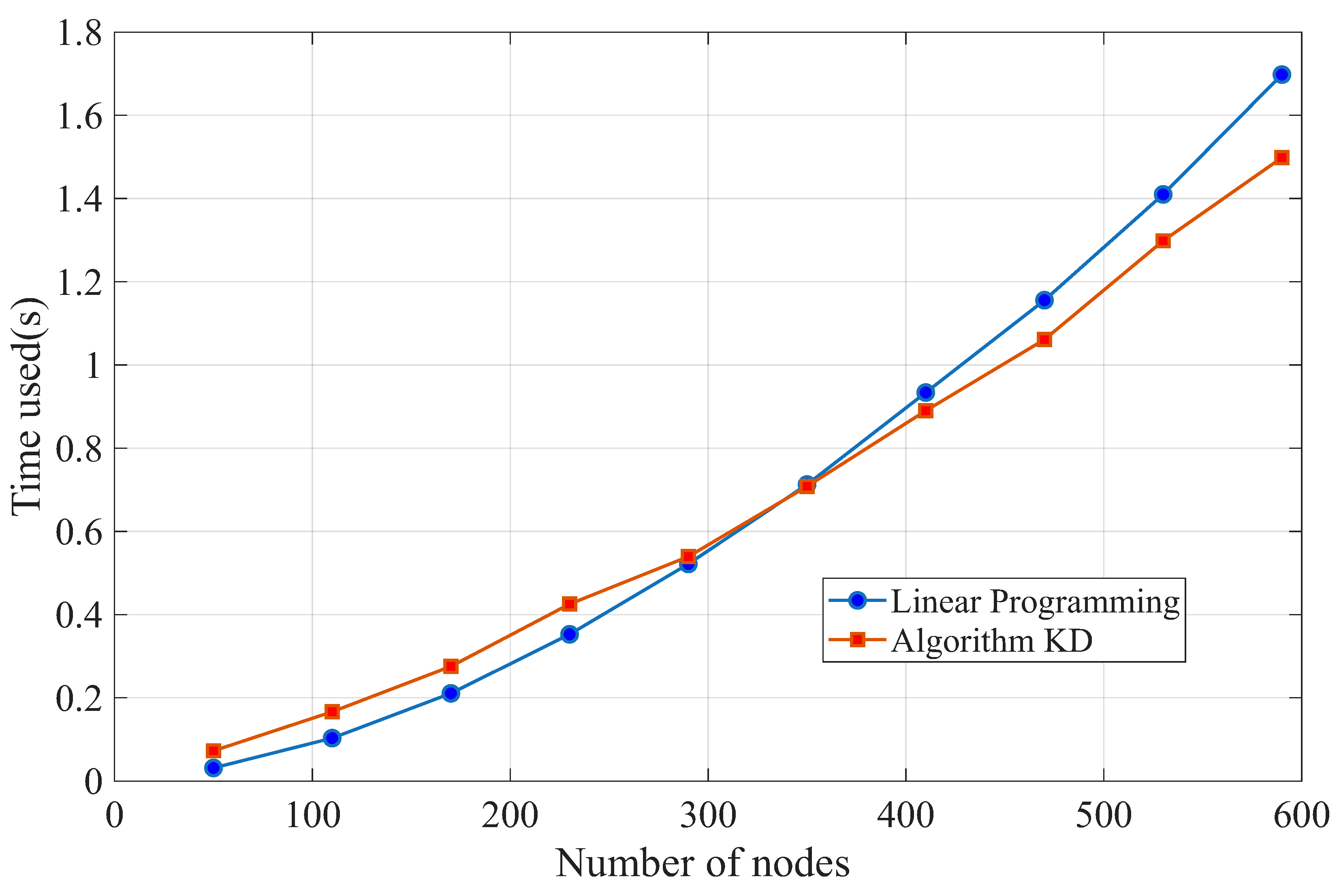
The mentioned algorithm is based on a greedy approach. It speeds up the project by only one day at a time, and repeats it k times. Each time it adopts the minimum cost strategy to shorten the project (by one day). This does not guarantee the minimum total cost when $k>1$ (see an example in Section 5.1). Nevertheless, it is a simple, efficient, and practical algorithm, which has been implemented in certain applications [3]. Therefore, a theoretical analysis of its approximation performance seems to be important and may benefit the relevant researchers and engineers. Such an analysis is not easy and is absent in the literature, hence we cover it in this paper.

1.1. Description of the k-Crashing Problem

A project is considered as an activity-on-edge network (AOE network, which is a directed acyclic graph) N, where each activity/job of the project is an edge. Some jobs must be finished before others can be started, as described by the topology structure of N.

It is known that job $j_i$ in normal speed would take $b_i$ days to be finished after it is started, and hence the (normal) duration of the project N, denoted by $d\left(N\right)$, is determined, which equals the length of the critical path (namely, the longest path) of N.

To speed up the project, the manager can crash a few jobs (namely, reduce the length of the corresponding edges) by investing extra resources into those jobs, such as deploying more staff, upgrading current procedures, and purchasing more equipment. However, the time for completing $j_i$ has a lower bound due to technological limits—it requires at least $a_i$ days to be completed. Following the convention, assume that the duration of a job has a linear relation with the extra resources put into this job; equivalently, there is a parameter $c_i$ (slope), so that shortening $j_i$ by $d(0\le d\le b_i-a_i)$ days costs $c_i·d$ resources.

Given project N and an integer $k\ge 1$, the k-crashing problem asks the minimum cost to speed up the project by k days.

In fact, many people also care about the case of non-linear relation, especially the convex case, where shortening an edge becomes more difficult after a previous shortening. Delightfully, the greedy algorithm performs equally well for this convex case. Without any change, it still finds a solution with the approximation ratio upper bound ${\displaystyle \frac{1}{1}}+\dots +{\displaystyle \frac{1}{k}}$.

1.2. Our Contribution and Paper Structure

The main contributions of this paper are as follows:

• We revisit a simple and efficient greedy algorithm for solving the k-crashing problem in project management, which aims to minimize the resources required to shorten a project’s duration by k days. We prove that this algorithm achieves an approximation ratio upper bound of ${\displaystyle \frac{1}{1}}+\dots +{\displaystyle \frac{1}{k}}$, providing a theoretical guarantee for its performance.
• We explore the generalization of the algorithm to the convex case, where the cost of shortening an edge increases as more resources are invested, and it shows that the approximation ratio upper bound remains valid in this more complex scenario.
• We extend the analysis to a similar problem, the k-extending problem, where the goal is to extend the shortest paths of a network by k days, and we prove that the same approximation ratio upper bound holds for this problem, demonstrating the generalizability of our analysis.

The conference version of this paper only involves the approximation ratio bound of the first contribution all other contributions are only demonstrated in this paper. We believe these contributions provide insights for project managers and researchers working on time-cost trade-offs in project scheduling.

The organization of this paper is as follows. In Section 2, we discuss the work related to our research. In Section 3, we prove the approximation ratio upper bound of ${\displaystyle \frac{1}{1}}+\dots +{\displaystyle \frac{1}{k}}$ for Algorithm KD in the original k-crashing problem. Then, in Section 4, we generalize the approximation ratio upper bound to the convex case where shortening an edge gets more and more costly as we shorten it. 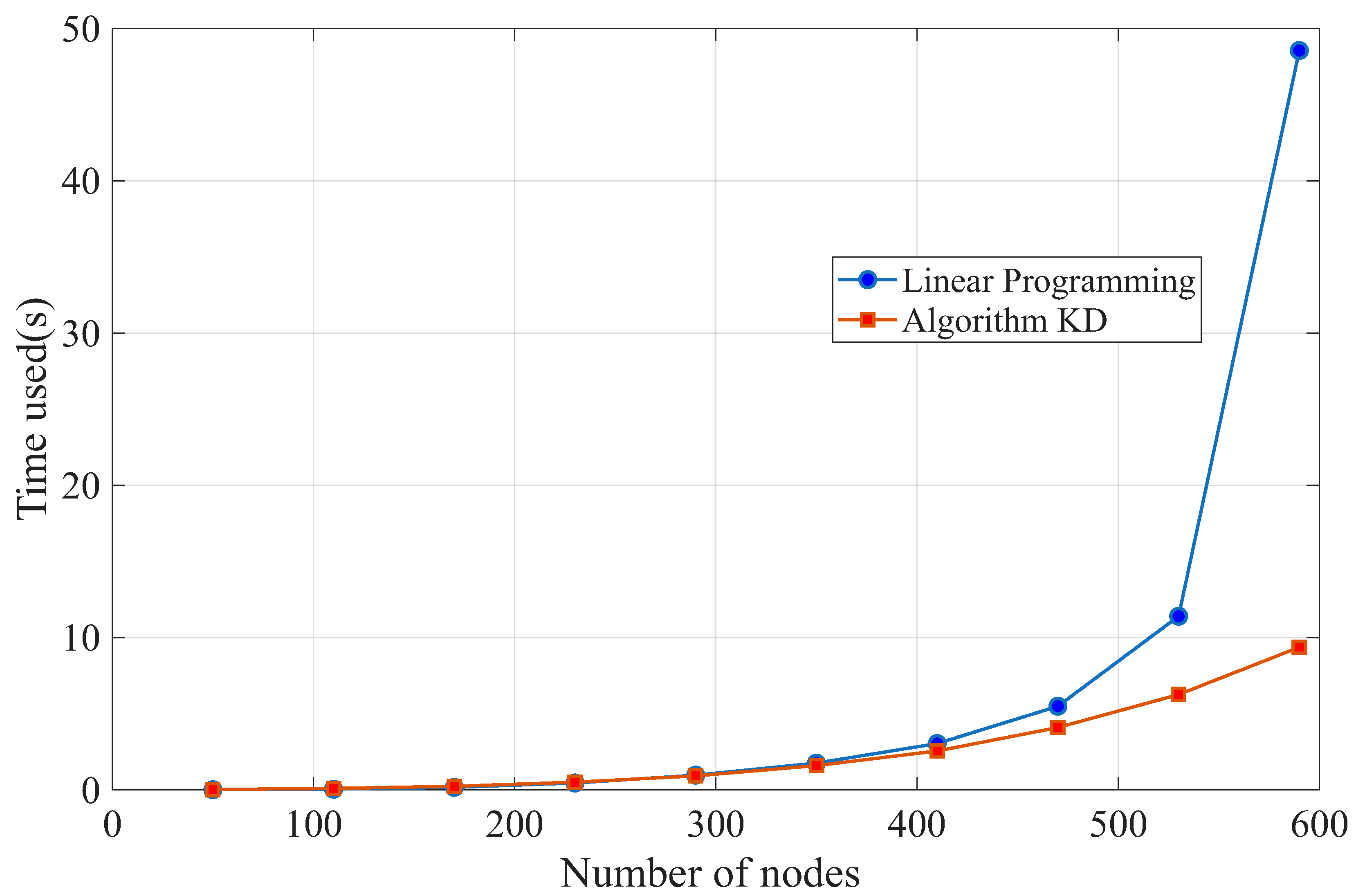Next, in Section 6, we discuss the tightness of our bound with a counterexample where Algorithm KD does not produce an optimum solution and demonstrate the experimental results reflecting the efficiency of Algorithm KD. In Section 6, we implement the same procedure and prove the same approximation ratio upper bound of ${\displaystyle \frac{1}{1}}+\dots +{\displaystyle \frac{1}{k}}$ for the greedy algorithm in the k-extending problem. Finally, in Section 7, we summarize our work from this paper and point out some of the possible directions for future research.

2. Related Work

The first solution to the k-crashing problem was given by Fulkerson [4] and by Kelley [5], respectively, in 1961. The results in these two papers are independent, yet the approaches are essentially the same, as pointed out in [6]. In both of them, the problem is first formulated into a linear program problem, whose dual problem is a minimum-cost flow problem, which can then be solved efficiently.

Later in 1977, Phillips and Dessouky [6] reported another clever approach (denoted by Algorithm PD). Similar to the greedy algorithm mentioned above, Algorithm PD also consists of k steps, and at each step it locates a minimal cut in a flow network derived from the original project network. This minimal cut is then utilized to identify the jobs which should be expedited or de-expedited in order to reduce the project reduction. It is however not clear whether this algorithm can always find an optimum solution (it is believed so in many sources [7,8,9,10]). We tend to believe the correctness yet cannot find a proof in [6].

It is noteworthy to mention that Algorithm PD shares a lot of common logic with the greedy algorithm we considered. Both of them locate a minimal cut in some flow network and then use it to identify the set of jobs to expedite/de-expedite in the next round. However, the constructed flow networks are different. The one in the greedy algorithm has only capacity upper bounds, whereas the one in Algorithm PD has both capacity upper bounds and lower bounds and is thus more complex.

Algorithm KD is simpler and easier to implement compared to all the approaches above. Since it is arguably the simplest algorithm for the problem, it has been brought up in the literature multiple times [2,11,12,13,14]. Compared with Algorithm PD, there is no de-expedite option allowed in Algorithm KD. As a result, for online cases where the project duration must be reduced optimally unit by unit (where each step must be the cheapest at the time) and the crashing is non-revocable, Algorithm KD can still be implemented but Algorithm PD cannot. So the approximation ratio of Algorithm KD can also be regarded as the price of “online” property, which is also known as the concept of competitive ratio studied for multiple problems, such as online allocation [15], linear search [16], chasing convex bodies [17], bin packing [18], online matching [19], and perimeter defense [20].

Other approaches for the problem are proposed by Siemens [1] and Goyal [21], but these are heuristic algorithms without any guarantee—approximation ratios are not proved in these papers.

Many variants of the k-crashing problem have been studied in the past decades; see [9,10,22,23], and the references within.

3. k-Crashing Problem

To begin with, we now introduce the basic notations and definitions needed for this research as follows.

Project N. 

Assume $N=(V,E)$ is a directed acyclic graph with a single source node s and a single sink node t (a source node refers to a node without incoming edge, and a sink node refers to a node without outgoing edges). Each edge $e_i\in E$ has three attributes $(a_i,b_i,c_i)$, as introduced in Section 1.1.

Critical paths and critical edges. 

A path of N refers to a path of N from source s to sink t. Its length is the total length of the edges included, and the length of edge $e_i$ equals $b_i$. The path of N with the longest length is called a critical path. The duration of N equals the length of the critical paths. There may be more than one critical path. An edge that belongs to some critical paths is called a critical edge.

Accelerate plan X. 

Denote by $E_{b\setminus a}$ the multiset of edges of N that contains $e_i$ with a multiplicity $b_i-a_i$. Each subset X of $E_{b\setminus a}$ (which is also a multiset) is called an accelerate plan, or plan for short. The multiplicity of $e_i$ in X, denoted by $x_i(0\le x_i\le b_i-a_i)$, describes how much length $j_i$ is shortened; i.e., $j_i$ takes $b_i-x_i$ days when plan X is applied. The cost of plan X, denoted by $\mathsf{cost}\left(X\right)$, is ${\sum }_i{c}_i{x}_i$.

Accelerated project $N\left(X\right)$. 

Define $N\left(X\right)$ as the project that is the same as N, but with $b_i$ decreased by $x_i$; in other words, $N\left(X\right)$ stands for the project optimized with plan X.

k-crashing. 

We say a plan X is k-crashing if the duration of the project N is shortened by k when we apply plan X.

Cut of N. 

Suppose that V is partitioned into two subsets $S,T$, which, respectively, contain s and t. Then, the set of edges from S to T is referred to as a cut of N. Notice that we cannot reach t from s if any cut of N is removed.

Let $k_{\max }$ be the duration of the original project N minus the duration of the accelerated project $N\left(E_{b\setminus a}\right)$. Clearly, the duration of $N\left(X\right)$ is at least the duration of $N\left(E_{b\setminus a}\right)$, since X is a subset of $E_{b\setminus a}$. It follows that a k-crashing plan only exists for $k\le k_{\max }$.

Throughout the paper, we assume that $k\le k_{\max }$.

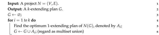
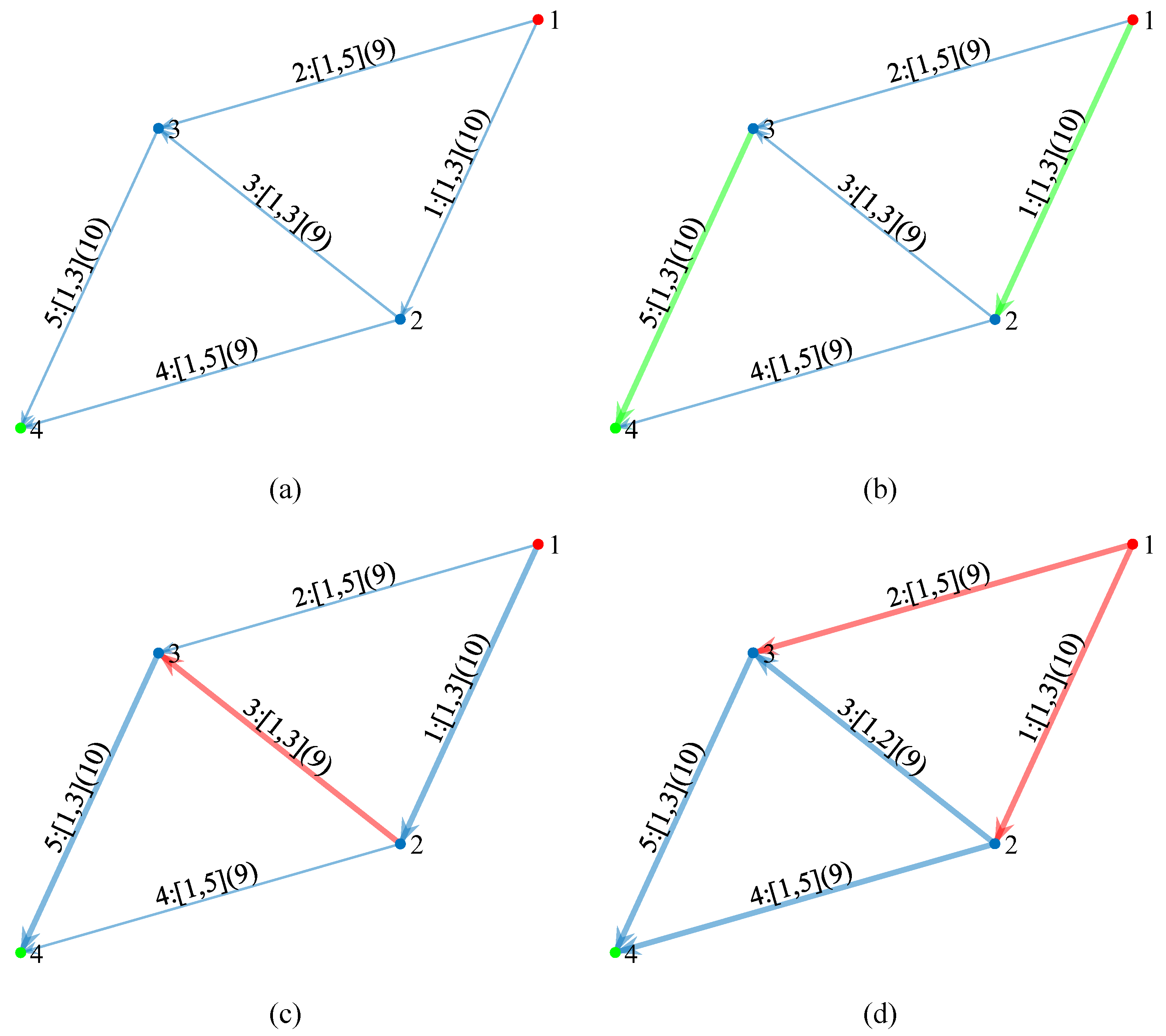
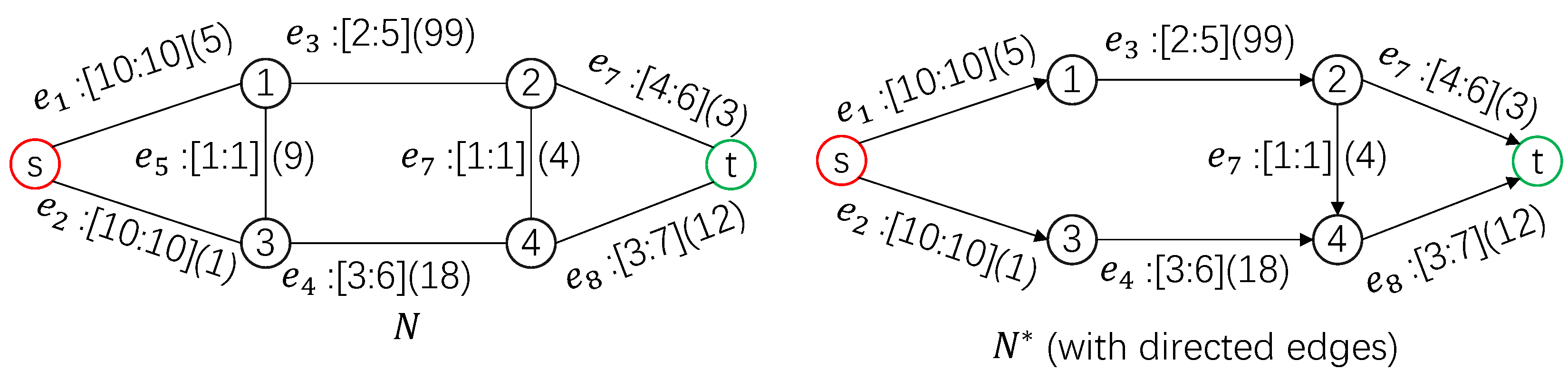
The greedy algorithm (Algorithm KD) in the following (see Algorithm 1) finds a k-crashing plan efficiently. It finds the plan incrementally—each time it reduces the duration of the project by 1. See Figure 1 for an example of a 1-crashing problem of a project network.

Algorithm 1: Greedy algorithm for finding a k-crashing plan.(Algorithm KD).

Observe that G is an i-crashing plan of N after the i-th iteration $G\leftarrow G\cup A_i$, as the duration of $N\left(G\right)$ is reduced by 1 at each iteration. Therefore, G is a k-crashing plan at the end.

If a 1-crashing plan of $N\left(G\right)$ does not exist in the i-th iteration $i\le k$, we determine that there is no k-crashing plan; i.e., $k>k_{\max }$.

Theorem 1. 

Let $G=A_1\cup \dots \cup A_k$ be the k-crashing plan found by Algorithm 1. Let $\mathsf{OPT}$ denote the optimum k-crashing plan. Then,

$$\mathsf{cost}\left(G\right)\le \sum _{i=1}^k{\displaystyle \frac{1}{i}}\mathsf{cost}\left(\mathsf{OPT}\right).$$

The proof of the theorem is given in the following, which applies Lemma 1. This applied lemma is nontrivial and is proven below.

Lemma 1. 

For any project N, its k-crashing plan (where $k\le k_{\mathit{max}}$) costs at least k times the cost of the optimum 1-crashing plan.

Proof of Theorem 1. 

For convenience, let $N_i=N(A_1\cup \dots \cup A_i)$, for $0\le i\le k$. Note that $N_0=N$ is the original project.

Fix i in $\{1,\dots ,k\}$ in the following. By the algorithm, $A_i$ is the optimum 1-crashing plan of $N_{i-1}$. Using Lemma 1, we know (1) any $(k+1-i)$-crashing plan of $N_{i-1}$ costs at least $(k+1-i)·\mathsf{cost}\left(A_i\right)$.

Let $Y=A_1\cup \dots \cup A_{i-1}$ and $X=\mathsf{OPT}\setminus Y$; hence $X\cup Y\supseteq \mathsf{OPT}$.

Observe that $N(Y\cup X)$ saves k days compared to N, because $Y\cup X\supseteq \mathsf{OPT}$ is k-crashing, whereas $N\left(Y\right)=N_{i-1}$ saves $i-1$ days compared to N. So, $N(Y\cup X)$ saves $k-(i-1)$ days compared to $N\left(Y\right)$, which means (2) X is a $(k-i+1)$-crashing plan of $N\left(Y\right)=N_{i-1}$. Combining (1) and (2), $\mathsf{cost}\left(X\right)\ge (k+1-i)\mathsf{cost}\left(A_i\right)$.

Furthermore, since $\mathsf{cost}\left(X\right)\le \mathsf{cost}\left(\mathsf{OPT}\right)$ (as $X\subseteq \mathsf{OPT}$), we obtain a relation $(k-i+1)\mathsf{cost}\left(A_i\right)\le \mathsf{cost}\left(\mathsf{OPT}\right)$. Therefore,

$$\mathsf{cost}\left(G\right)=\sum _{i=1}^k\mathsf{cost}\left(A_i\right)\le \sum _{i=1}^k{\displaystyle \frac{1}{k-i+1}}\mathsf{cost}\left(\mathsf{OPT}\right).$$

   □

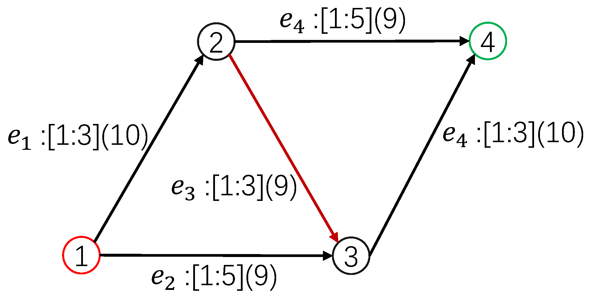
The critical graph of network H, denoted by $H^{*}$, is formed by all the critical edges of H; all the edges that are not critical are removed in $H^{*}$.

Before presenting the proof to the key lemma (Lemma 1), we shall briefly explain how we find the optimum 1-crashing plan of some project H (e.g., the accelerated project $N\left(G\right)$ in Algorithm 1). First, compute the critical graph $H^{*}$ and define the capacity of $e_i$ in $H^{*}$ by $c_i$ if $e_i$ in H can still be shortened (i.e., its length is more than $a_i$); otherwise, define the capacity of $e_i$ in $H^{*}$ to be ∞. Then we compute the minimum $s-t$ cut of $H^{*}$ (using the max-flow algorithm [24]), and this cut gives the optimum 1-crashing plan of H.

3.1. Proof (Part I)

Proposition 1. 

A k-crashing plan X of N contains a cut of $N^{*}$.

Proof. 

Because X is k-crashing, each critical path of N will be shortened in $N\left(X\right)$, and that means it contains an edge of X. Furthermore, since the paths of $N^{*}$ are critical paths of N (which simply follows from the definition of $N^{*}$), each path of $N^{*}$ contains an edge in X.

As a consequence, after removing the edges in X that belong to $N^{*}$, we disconnect source s and sink t in $N^{*}$. Now, let S denote the vertices of $N^{*}$ that can still be reached from s after removal, and let T denote the remaining part. Observe all edges from S to T in $N^{*}$ which form a cut of $N^{*}$ that belongs to X.    □

When X contains at least one cut of network H, let $\mathsf{mincut}(H,X)$ be the minimum cut of H among all cuts of H that belong to X.

Recall that $d\left(H\right)$ is the duration of network H.

In the following, suppose X is a k-crashing plan of N. We introduce a decomposition of X which is crucial to our proof.

First, define

$$\left\{\begin{array}{ccc}{N}_1& =& N,\\ X_1& =& X,\\ C_1& =& \mathsf{mincut}(N_1^{*},X_1).\end{array}\right.$$

(1)

(Because $X_1=X$ is k-crashing, applying Proposition 1, $X_1$ contains at least one cut of $N_1^{*}$. It follows that $C_1$ is well-defined.)

Next, for $1<i\le k$, define

$$\left\{\begin{array}{ccc}{N}_i& =& N_{i-1}^{*}\left(C_{i-1}\right),\\ X_i& =& X_{i-1}\setminus C_{i-1}.\\ C_i& =& \mathsf{mincut}(N_i^{*},X_i).\end{array}\right.$$

(2)

See Figure 2 for an example.

Proposition 2. 

For $1<i\le k$, it holds that

1. $d\left(N_i\right)=d\left(N_{i-1}\right)-1$ (namely, $d\left(N_i\right)=d\left(N\right)-i+1$).

2. $X_i$ contains a cut of $N_i^{*}$ (and thus $C_i$ is well-defined).

Proof. 

1. Because $C_{i-1}$ is a cut of $N_{i-1}^{*}$, set $C_{i-1}$ is a 1-crashing plan of $N_{i-1}^{*}$, which means $d\left(N_{i-1}^{*}\left(C_{i-1}\right)\right)\le d\left(N_{i-1}^{*}\right)-1$.

Moreover, $d\left(N_{i-1}^{*}\left(C_{i-1}\right)\right)\le d\left(N_{i-1}^{*}\right)-2$ cannot hold. Otherwise, cancel one edge of $C_{i-1}$ and $d\left(N_{i-1}^{*}\left(C_{i-1}\right)\right)\le d\left(N_{i-1}^{*}\right)-1$ still holds, which means $C_{i-1}$ is at least 1-crashing for $N_{i-1}^{*}$, and thus contains a cut of $N_{i-1}^{*}$ (by Proposition 1). This contradicts the assumption that $C_{i-1}$ is the minimum cut.

Therefore, $d\left(N_i\right)=d\left(N_{i-1}^{*}\left(C_{i-1}\right)\right)=d\left(N_{i-1}^{*}\right)-1=d\left(N_{i-1}\right)-1$.

2. According to Proposition 1, it is sufficient to prove that $X_i$ is a 1-crashing plan to $N_i$.

Suppose the opposite, where $X_i$ is not 1-crashing to $N_i$. There exists a path P in $N_i^{*}$ that is disjoint with $X_i$. Observe that

(1) The length of P in $N\left(X\right)$ is the original length of P (in N) minus the number of edges in X that fall in P.

(2) The length of P in $N_i^{*}$ is the original length of P (in N) minus the number of edges in $(C_1\cup \dots \cup C_{i-1})$ that fall in P.

(3) The number of edges in $(C_1\cup \dots \cup C_{i-1})$ that fall in P equals the number of edges in X that fall in P, because $X\setminus (C_1\cup \dots \cup C_{i-1})=X_i$ is disjoint with P.

Together, the length of P in $N\left(X\right)$ equals the length of P in $N_i^{*}$, which equals $d\left(N_i^{*}\right)=d\left(N_i\right)=d\left(N\right)-i+1>d\left(N\right)-k$. This means X is not a k-crashing plan of P, contradicting our assumption. □

The following lemma easily implies Lemma 1.

Lemma 2. 

$\mathsf{cost}\left(C_i\right)\le \mathsf{cost}\left(C_{i+1}\right)$ for any $i(1\le i<k)$.

We show how to prove Lemma 1 in the following. The proof of Lemma 2 will be shown in the next subsection.

Proof of Lemma 1. 

Suppose X is k-crashing to N.

By Lemma 2, we know $\mathsf{cost}\left(C_1\right)\le \mathsf{cost}\left(C_i\right)(1\le i\le k)$.

Furthermore, since ${\bigcup }_{i=1}^k{C}_i\subseteq X$,

$$k·\mathsf{cost}\left(C_1\right)\le \mathsf{cost}\left(\bigcup _{i=1}^k{C}_i\right)\le \mathsf{cost}\left(X\right).$$

Because $C_1$ is the minimum cut of $N^{*}$ that is contained in X, whereas $A_1$ is the minimum cut of $N^{*}$ among all, $\mathsf{cost}\left(A_1\right)\le \mathsf{cost}\left(C_1\right)$. To sum up, we have $k·\mathsf{cost}\left(A_1\right)\le \mathsf{cost}\left(X\right).$    □

It is noteworthy to mention that ${\bigcup }_{i=1}^k{C}_i$ is not always equal to X and ${\bigcup }_{i=1}^k{C}_i$ may not be k-crashing.

3.2. Proof (Part II)

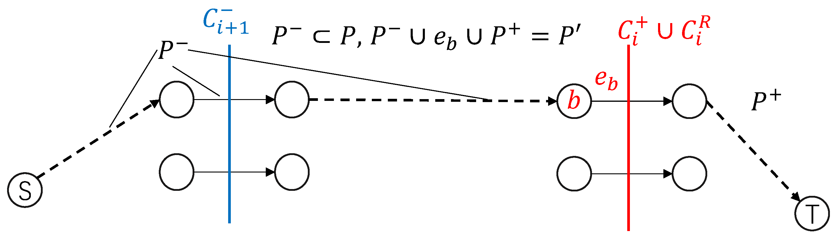
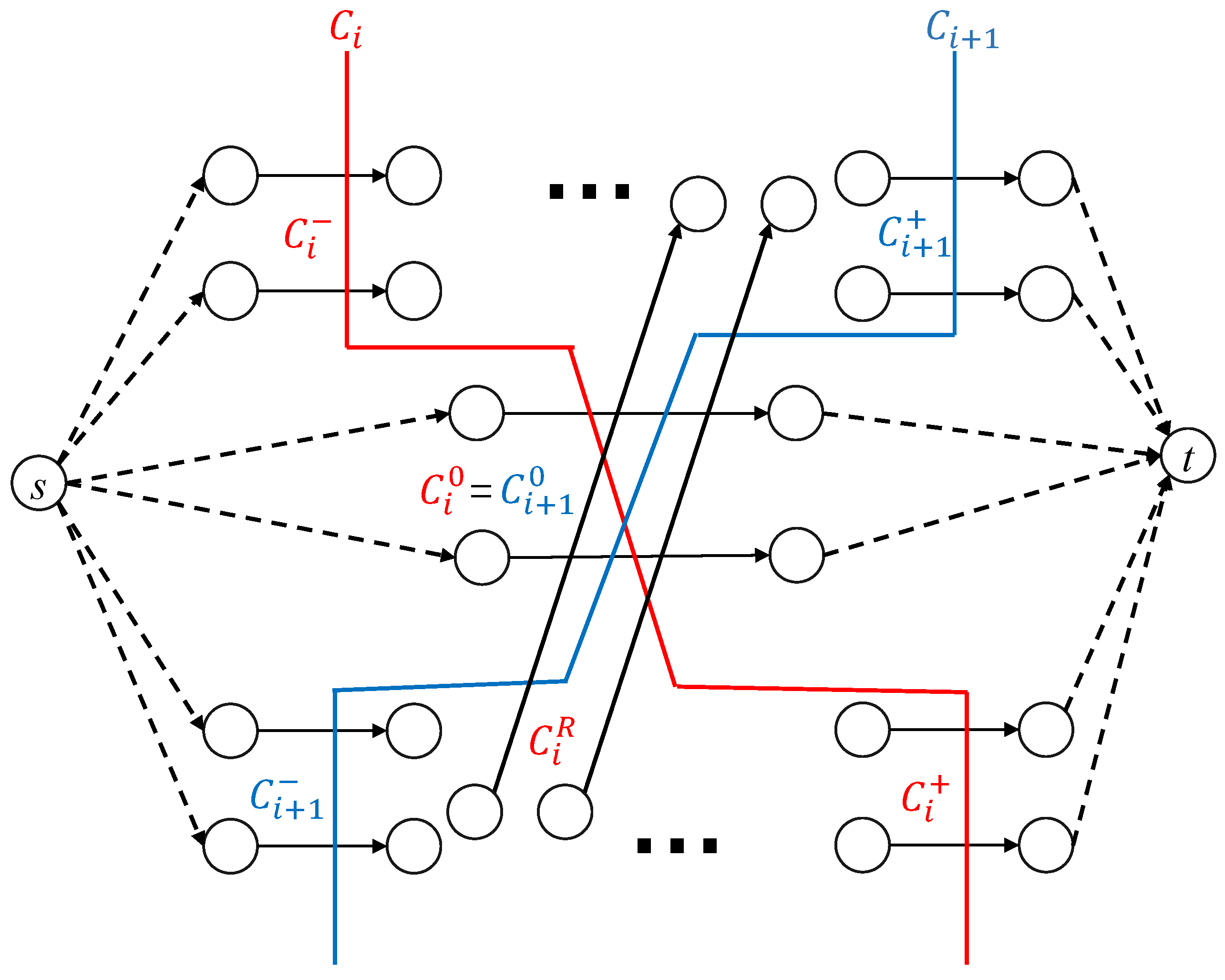
Assume $i(1\le i<k)$ is fixed. In the following we prove that $\mathsf{cost}\left(C_i\right)\le \mathsf{cost}\left(C_{i+1}\right)$, as stated in Lemma 2. Some additional notation shall be introduced here. See Figure 3 and Figure 4.

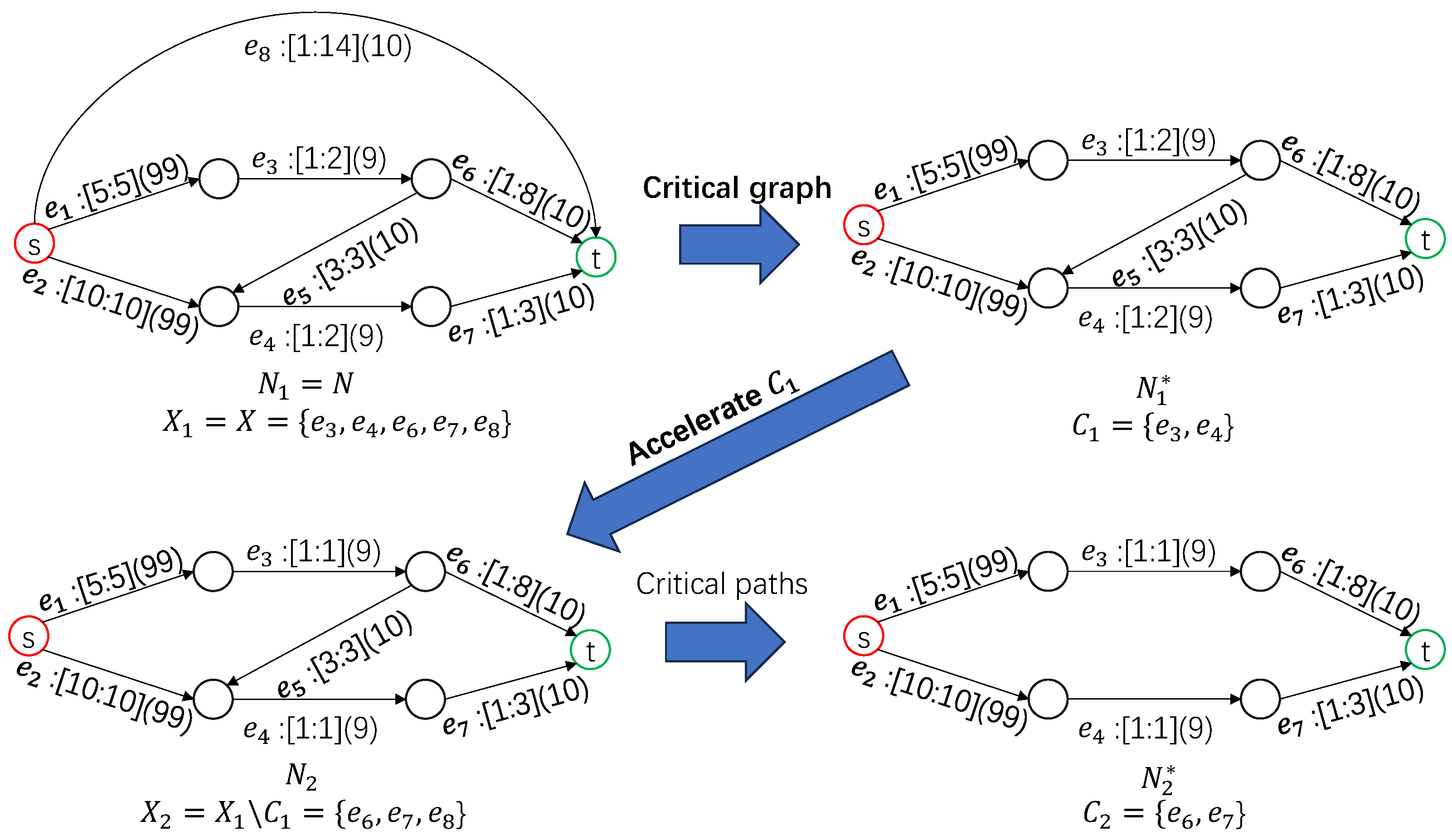
Assume the cut $C_i$ of $N_i^{*}$ divides the vertices of $N_i^{*}$ into two parts, $U_i,W_i$, where $s\in U_i$ and $t\in W_i$. The edges of $N_i^{*}$ are divided into four parts as follows: 1. $S_i$—the edges within $U_i$; 2. $T_i$—the edges within $W_i$; 3. $C_i$—the edges from $U_i$ to $W_i$; and 4. $R{C}_i$—the edges from $W_i$ to $U_i$.

Proposition 3.

(1) $C_{i+1}\cap R{C}_i=\varnothing$ and (2) $C_i\subseteq N_{i+1}^{*}$.

Proof. 

(1) Consider $N_i^{*}$. Any path involving $R{C}_i$ goes through $C_i$ at least twice. Such paths are shortened by $C_i$ by at least 2 and are thus excluded from $N_{i+1}$. However, $C_{i+1}$ are the edges in $N_{i+1}^{*}$ and so are included in $N_{i+1}$. Together, $C_{i+1}\cap R{C}_i=\varnothing$.

(2) Suppose there is an edge $e_i\in C_i$ and $e_i\notin N_{i+1}^{*}$. All paths in $N_i^{*}$ passing $e_i$ will be shortened by at least 2 after expediting $C_i$ to avoid becoming a critical path (which makes $e_i$ critical). If the shortening of $e_i$ is canceled, the paths can still be shortened by 1. So $C_i\setminus \left\{e_i\right\}$ still contains a cut to $N_i^{*}$, which violates the assumption that $C_i$ is the minimum cut and is contradictory. So $C_i\subseteq N_{i+1}^{*}$.    □

Because $C_{i+1}$ is a subset of the edges of $N_{i+1}^{*}$, and the edges of $N_{i+1}^{*}$ are also in $N_i^{*}$, we see $C_{i+1}\subseteq T_i\cup S_i\cup C_i\cup R{C}_i$. Furthermore, since $C_{i+1}\cap R{C}_i=\varnothing$ (Proposition 3), set $C_{i+1}$ consists of the following three disjoint parts:

$$\left\{\begin{array}{cc}\hfill C_{i+1}^{+}& =C_{i+1}\cap T_i;\hfill \\ \hfill C_{i+1}^0& =C_{i+1}\cap C_i;\hfill \\ \hfill C_{i+1}^{-}& =C_{i+1}\cap S_i.\hfill \end{array}\right.$$

(3)

Due to $C_i\subseteq N_{i+1}^{*}$ (Proposition 3), set $C_i$ consists of four disjoint parts as follows:

$$\left\{\begin{array}{cc}\hfill C_i^{+}& =C_i\cap T_{i+1}\hfill \\ \hfill C_i^0& =C_i\cap C_{i+1}\hfill \\ \hfill C_i^{-}& =C_i\cap S_{i+1}\hfill \\ \hfill C_i^R& =C_i\cap R{C}_{i+1}\hfill \end{array}\right.$$

(4)

See Figure 4 for an illustration. Note that $C_i^0=C_{i+1}^0$.

Proposition 4. 

 

1. $C_{i+1}^{+}\cup C_i^0\cup C_i^{+}$ contains a cut of $N_i^{*}$.

2. $C_{i+1}^{-}\cup C_i^0\cup C_i^{-}$ contains a cut of $N_i^{*}$.

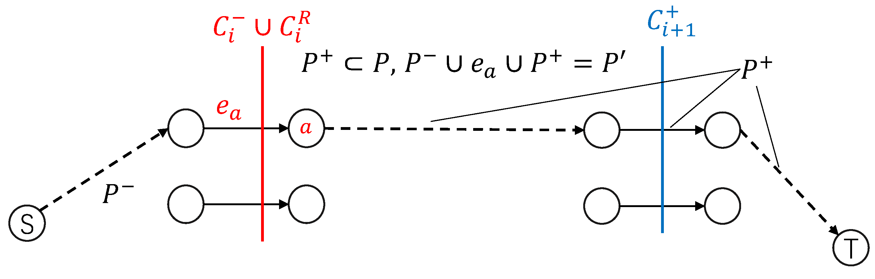
Proof. 

To show that $C_{i+1}^{+}\cup C_i^0\cup C_i^{+}$ contains a cut of $N_i^{*}$, it is sufficient to prove that any path P in $N_i^{*}$ goes through $C_{i+1}^{+}\cup C_i^0\cup C_i^{+}$.

Assume that P is disjoint with $C_i^{+}\cup C_i^0$; otherwise, it is trivial. We shall prove that P goes through $C_{i+1}^{+}$.

Clearly, P goes through $C_i=C_i^{+}\cup C_i^0\cup C_i^{-}\cup C_i^R$, a cut of $N_i^{*}$. Therefore, P goes through $C_i^{-}\cup C_i^R$. See Figure 5.

Take the last edge in $C_i^{-}\cup C_i^R$ that P goes through; denoted by $e_a$ with endpoint a. Denote the part of P after $e_a$ by $P^{+}$ ($P^{+}\cap C_i=\varnothing$).

We now claim that

(1) $P^{+}\subseteq T_i$.

(2) In $N_i^{*}$, there must be a path $P^{-}\subseteq S_i$ from the source to $e_a$ that does not pass through $C_i$ ($P^{-}\cap C_i=\varnothing$).

(3) $a\in U_{i+1}$.

Since P is disjoint with $C_i^{+}\cup C_i^0$ and $P^{+}$ has gone through $C_i^{-}\cup C_i^R$, we obtain (1).

If (2) does not hold, then all paths in $N_i^{*}$ that pass through $e_a$ have passed through $C_i$ already. In this case, $C_i\setminus e_a$ also contains a cut of $N_i^{*}$, which contradicts our definition of minimum cut $C_i$. Thus, we have (2).

By definition (4), any edge of $C_i^{-}\cup C_i^R$ ends at a vertex of $U_{i+1}$. Since a is the endpoint of $e_a\in C_i^{-}\cup C_i^R$, we have (3).

By (2), we can obtain a $P^{-}$ from s to $e_a$. Concatenating $P^{-},e_a,P^{+}$, we obtain a path $P^{\prime }$ in $N_i^{*}$. $(P^{-}\cup P^{+})\cap C_i=\varnothing$ and $e_a\in C_i$, $P^{\prime }$ only goes through $C_i^{-}\cup C_i^R$ once. So $P^{\prime }$ is only shortened by 1 and is still critical after expediting $C_i$. Therefore, $P^{\prime }$ exists in $N_{i+1}^{*}$.

According to (3), we know that $P^{+}\in P^{\prime }$ starts with $a\in U_{i+1}$ and ends at the sink in $W_{i+1}$. Thus, it must go though cut $C_{i+1}$.

According to (1) and definition (3), path $P^{+}$ (which is a subset of $T_i$ due to (1)) can only go through $C_{i+1}^{+}\subset T_i$.

Since $P^{+}\subset P$, we know that P goes through $C_{i+1}^{+}$. So any path P in $N_i^{*}$ goes through $C_{i+1}^{+}\cup C_i^0\cup C_i^{+}$.

Therefore, $C_{i+1}^{+}\cup C_i^0\cup C_i^{+}$ contains a cut of $N_i^{*}$.

Symmetrically, we can show that $C_{i+1}^{-}\cup C_i^0\cup C_i^{-}$ contains a cut of $N_i^{*}$,    □

We are ready to prove Lemma 2.

Proof of Lemma 2. 

According to Proposition 4, $C_{i+1}^{+}\cup C_i^0\cup C_i^{+}$ and $C_i^{-}\cup C_i^0\cup C_{i+1}^{-}$ each contain a cut of $N_i^{*}$. Notice that $((C_{i+1}^{+}\cup C_i^0\cup C_i^{+})\cup (C_i^{-}\cup C_i^0\cup C_{i+1}^{-})\cup C_i^R)=(C_i\cup C_{i+1})\subset X_i$, so the mentioned two cuts are in $X_i$. Furthermore, since $C_i$ is the minimum cut of $N_i^{*}$ in $X_i$. We obtain

$$\begin{array}{cc}\hfill \mathsf{cost}\left(C_i\right)& =\mathsf{cost}(C_i^{+}\cup C_i^0\cup C_i^{-}\cup C_i^R)\le \mathsf{cost}(C_{i+1}^{+}\cup C_i^0\cup C_i^{+})\hfill \\ \hfill \mathsf{cost}\left(C_i\right)& =\mathsf{cost}(C_i^{+}\cup C_i^0\cup C_i^{-}\cup C_i^R)\le \mathsf{cost}(C_{i+1}^{-}\cup C_i^0\cup C_i^{-})\hfill \end{array}$$

By adding the inequalities above (and noting that $C_{i+1}^0=C_i^0=C_i\cap C_{i+1}$), we have

$$\begin{array}{cc}\hfill & 2\mathsf{cost}(C_i^{+}\cup C_i^0\cup C_i^{-}\cup C_i^R)\le \hfill \\ \hfill & \mathsf{cost}(C_{i+1}^{+}\cup C_i^0\cup C_i^{+})+\mathsf{cost}(C_i^{-}\cup C_{i+1}^0\cup C_{i+1}^{-})\hfill \end{array}$$

Equivalently,

$$\begin{array}{cc}\hfill & 2\mathsf{cost}(C_i^{+}\cup C_i^0\cup C_i^{-})+2\mathsf{cost}\left(C_i^R\right)\le \hfill \\ \hfill & \mathsf{cost}(C_i^{-}\cup C_i^0\cup C_i^{+}\cup C_{i+1}^{+}\cup C_{i+1}^0\cup C_{i+1}^{-}).\hfill \end{array}$$

By removing one piece of $\mathsf{cost}(C_i^{-}\cup C_i^0\cup C_i^{+})$ from both sides,

$$\mathsf{cost}\left(C_i\right)+\mathsf{cost}\left(C_i^R\right)\le \mathsf{cost}(C_{i+1}^{+}\cup C_{i+1}^0\cup C_{i+1}^{-})=\mathsf{cost}\left(C_{i+1}\right)$$

Therefore, $\mathsf{cost}\left(C_i\right)\le \mathsf{cost}\left(C_{i+1}\right)$.    □

Besides, with Lemma 2, we can now prove that the cost of the greedy steps is incremental during Algorithm 1.

Corollary 1. 

For neighboring greedy steps $A_i$ and $A_{i+1}$, we have $\mathsf{cost}\left(A_i\right)\le \mathsf{cost}\left(A_{i+1}\right)$.

Proof. 

Note that any neighboring greedy steps $A_i$ and $A_{i+1}$ can be seen as the two greedy steps of a 2-crashing problem. Therefore, we can reduce it to proving that $\mathsf{cost}\left(A_1\right)\le \mathsf{cost}\left(A_2\right)$ for any 2-crashing problem.

In this case, recall the definitions related to Lemma 2. We now let $k=2$ and X be the greedy solution for the 2-crashing problem. Naturally, we have $A_1\subseteq X$ and $A_2=X\setminus A_1$. By definition, we know that $A_1=C_1$ and $C_1\cup C_2\subseteq X$. Then, we have $C_2\subseteq X\setminus C_1=X\setminus A_1=A_2$.

By Lemma 2, we know that $\mathsf{cost}\left(C_1\right)\le \mathsf{cost}\left(C_2\right)$. Since $A_1=C_1$ and $C_2\subseteq A_2$, we have $\mathsf{cost}\left(A_1\right)=\mathsf{cost}\left(C_1\right)\le \mathsf{cost}\left(C_2\right)\le \mathsf{cost}\left(A_2\right)$.    □

With the upper bound of cost for Algorithm 1 (i.e., Theorem 1) and Corollary 1, we can also obtain the lower bound of k for the greedy algorithm when the budget is fixed and the target k is not.

For this symmetric problem, we describe the algorithm as follows.

Note that Algorithms 1 and 2 are essentially the same procedure. The difference is merely the termination condition of the loop. Therefore, for the same k-crashing result, they deliver exactly the same plan. Then, for the k in Algorithm 2, we have the following corollary. (For simplicity, we use the harmonic number $H\left(n\right)={\sum }_{i=1}^n{\displaystyle \frac{1}{i}}$ below.)    

Algorithm 2: Greedy algorithm for finding a crashing plan with a limited budget a.

Corollary 2. 

For budget a, project $N=(V,E)$. Suppose we can shorten the network by $k_1$ with Algorithm 2 and by $k_2$ in the optimum solution. We have

$${\displaystyle \frac{k_2}{H\left(k_2\right)}}-1\le k_1.$$

Proof. 

Suppose Algorithm 2 can deliver a $k_2$-crashing plan with a budget of at least x. Since Algorithm 1 delivers the same plan for the $k_2$-crashing problem, by Theorem 1, we have

$$x\le H\left(k_2\right)a.$$

Then by Corollary 1, we know that the cost of greedy steps is incremental. Then the average cost of the greedy procedure is incremental as well. Therefore, we have

$${\displaystyle \frac{a}{k_1+1}}\le {\displaystyle \frac{x}{k_2}}.$$

Together we have

$$a{k}_2\le x(k_1+1)\le H\left(k_2\right)a(k_1+1)$$

Thus,

$${\displaystyle \frac{k_2}{H\left(k_2\right)}}-1\le k_1.$$

   □

4. Generalization for the Convex Case

Recall the “convex case” mentioned in Section 1.1, in which shortening an edge becomes more and more expensive. More formally, for a crashing plan X, we have $\mathsf{cost}\left(X\right)={\sum }_i{\sum }_{j=1}^{x_i}{c}_{i,j}$, where $c_{i,j}$ indicates the cost of shortening the j th unit of edge i and $c_{i,j}\le c_{i,j+1}$. We claim that

Theorem 2. 

Let $G=A_1\cup \dots \cup A_k$ be the k-crashing plan found by Algorithm 1 in the convex case. Let $\mathsf{OPT}$ denote the optimum k-crashing plan in the convex case. Then,

$$\mathsf{cost}\left(G\right)\le \sum _{i=1}^k{\displaystyle \frac{1}{i}}\mathsf{cost}\left(\mathsf{OPT}\right).$$

Proof. 

First, let us start regarding the function $\mathsf{cost}(*)$ as the evaluation of the cost of a multiset of edges when they are applied to the original network N.

Now, recalling the definition of $N_i^{*}$, we define $\mathsf{cost}(A,i)$ by evaluating each edge in A according to their current cost in $N_i^{*}$ only. So the cost function $\mathsf{cost}(*,i)$ is fixed and linear for every $i(1\le i<k)$.

Therefore, by keeping the cost function fixed and linear as $\mathsf{cost}(*,i)$, we can directly apply Lemma 2 to obtain

$$\mathsf{cost}(C_i,i)\le \mathsf{cost}(C_{i+1},i)\mathrm{for}\mathrm{any}i(1\le i<k).$$

Note that $\mathsf{cost}(\left(C_{i+1}\right),i)\le \mathsf{cost}(\left(C_{i+1}\right),i+1)$ in the convex case since the edges become more and more expensive as we keep shortening the edges. We further have

$$\mathsf{cost}(\left(C_i\right),i)\le \mathsf{cost}(\left(C_{i+1}\right),i+1).$$

Since $A_1$ is the minimum cut of $N_1^{*}$, we have $\mathsf{cost}\left(A_1\right)\le \mathsf{cost}\left(C_1\right)=\mathsf{cost}(C_1,1)$. Thus, by $\mathsf{cost}(C_i,i)\le \mathsf{cost}(C_{i+1},i+1)$ and ${\bigcup }_{i=1}^k{C}_i\subseteq X$, we have

$$k·\mathsf{cost}\left(A_1\right)\le k·\mathsf{cost}\left(C_1\right)\le \sum _{i=1}^k\mathsf{cost}(C_i,i)\le \mathsf{cost}\left(X\right).$$

Let $X=\mathsf{OPT}$, we have

$$\mathsf{cost}\left(A_1\right)\le {\displaystyle \frac{1}{k}}·\mathsf{cost}\left(\mathsf{OPT}\right).$$

Since $A_i$ can be seen as the $A_1$ for a $(k-i+1)$-crashing problem and $\mathsf{OPT}$ contains a plan for the $(k-i+1)$-crashing problem. We can derive

$$\mathsf{cost}\left(G\right)=\sum _{i=1}^k\mathsf{cost}\left(A_i\right)\le \sum _{i=1}^k{\displaystyle \frac{1}{k-i+1}}\mathsf{cost}\left(\mathsf{OPT}\right)=\sum _{i=1}^k{\displaystyle \frac{1}{i}}\mathsf{cost}\left(\mathsf{OPT}\right).$$

Therefore, in the convex case, the approximation ratio upper bound ${\displaystyle \frac{1}{1}}+\dots +{\displaystyle \frac{1}{k}}$ still holds.    □

5. Constructive and Experimental Results

In this section, we present the results we obtained by constructing instances or running experiments to further demonstrate the properties of Algorithm 1.

5.1. Counterexample of Algorithm 1 and Tightness of the Bound

Algorithm 1 does not always find an optimum k-crashing plan. Here we first show an example.

The network is as shown in Figure 6a, and we consider $k=2$. The critical path of this network has length 9. The unique critical path consists of jobs $j_1$, $j_3$, and $j_5$.

Algorithm KD expedites job $j_3$ for one day in the first iteration; see Figure 6c. It further expedites jobs $j_1$ and $j_2$ for one day in the second iteration; see Figure 6d. The total cost is $9+9+10=28$.

The optimum k-crashing plan is to expedite jobs $j_1$ and $j_5$, as shown in Figure 6b, which costs $10+10=20$.

In fact, we let the cost of job $j_2,j_3$, and $j_5$ be x instead of 9. We have the ratio between Algorithm KD’s result and the optimum solution as

$${\displaystyle \frac{10+2x}{20}}.$$

As x approaches 10, we have limit

$$\underset{x\to 10}{lim}{\displaystyle \frac{10+2x}{20}}=1.5,$$

which matches the approximation ratio upper bound of $1+{\displaystyle \frac{1}{2}}=1.5$ for $k=2$. However, we find it difficult to construct a counterexample that matches the approximation ratio upper bound for cases where $k\ge 3$. So the tightness of this approximation ratio upper bound for $k\ge 3$ remains open. We conjecture that the upper bound obtained in the paper may have overly relaxed in the summation process of the proof of Theorem 1, and perhaps more properties can be found to further limit the upper bound for $k>2$.

In terms of approximation ratios, in certain cases, the worst case we ever know lies in [2], but the k is relatively large and the approximation ratio of the case becomes constant when k approaches infinity.

5.2. Experimental Results and Analysis

Algorithm KD repeatedly finds and crashes the minimum cut of the current critical graph to obtain the results. Let $T(m,n)$ denote the time required to search for the minimum cut (maximum flow) in a graph. Algorithm KD takes $kT(m,n)$ time to obtain a solution. Here, we regard $T(m,n)$ as $O\left(mn\right)$ [25] and thus obtain an $O\left(kmn\right)$ ($O\left(mn\right)$ when k is a constant) time bound for Algorithm KD. On the other hand, as is known in the literature [4], a k-crashing problem can also be solved by linear programming (denoted by LP), obtaining an optimum k-crashing plan. To the best of our knowledge, solving such a linear programming problem is currently still $O({(m+n)}^{2+\frac{1}{18}})$ [26]. So Algorithm KD is faster than LP when k is limited, which is not uncommon in practice.

To demonstrate the efficiency of Algorithm KD in practice, when k is small, we compare the efficiency between Algorithm KD and LP on randomly generated directed acyclic graphs when $k=2$. The default max-flow algorithm and interior point method of MATLAB (latest v. R2025a) are implemented, respectively. The results are shown in Figure 7 and Figure 8 for dense graphs and sparse graphs with n nodes and m edges (parameters’ distributions are shown in

Table 1. Data generation method.

Parameters	Distribution
Current duration $b_i$	[10, 50]
Minimum duration $a_i$	[1, $b_i$]
Crash cost $c_i$	[1, 10]

).

As is shown in Figure 7 and Figure 8, as the scale of the graph increases, the time used by LP increases faster than Algorithm KD’s. Besides, Algorithm KD produces the optimum result in all the 1000 instances, indicating that although Algorithm KD does not guarantee an optimum solution, it produces an optimum solution with high probability when $k=2$.

For cases of a larger k, the runtime of Algorithm KD would be proportional to k and the performance of LP would not be affected since k is just one single constraint. So we expect the figure to be visually the same except that the line of Algorithm KD goes upward proportionally to k compared with Figure 7 and Figure 8 for larger k. Since the theoretical time bound for $LP$ has larger exponents for m and n, as the size of the graph increases, the runtime of LP would always overtake Algorithm KD’s at some point.

6. k-Extending Problem

In Section 3, we have proven the upper bound of Algorithm KD in k-crashing problem. The result naturally leads us to a similar problem. With most of the notations unchanged, we now consider the network to be not directed in this k-extending problem. In this problem, we try to extend the length of the project (i.e., lengthening all the shortest paths (from s to t) in the network). This problem actually shares a lot of properties in common with the k-crashing problem. Using a similar technique, we can obtain the same $H\left(k\right)$ upper bound for the greedy algorithm of the k-extending problem below.

Here are some notations that have changed in this section compared with the k-crashing context.

Project N. 

Assume $N=(V,E)$ is a directed acyclic graph with a single source node s and a single sink node t. Each edge $e_i\in E$ has three attributes $(a_i,b_i,c_i)$, where $a_i$ denotes its current duration, $b_i$ denotes its maximum durations, and $c_i$ denotes its cost per unit extension.

Shortest paths and critical edges. 

The path from s to t with the shortest length is called the shortest path. The duration of N equals the length of the shortest paths. There may be more than one shortest path. An edge that belongs to some of the shortest paths is called a critical edge.

Extend plan X. 

Denote by $E_{b\setminus a}$ the multiset of the edges of N that contains $e_i$ with a multiplicity $b_i-a_i$. Each subset X of $E_{b\setminus a}$ (which is also a multiset) is called an extend plan, or plan for short. The multiplicity of $e_i$ in X, denoted by $x_i(0\le x_i\le b_i-a_i)$, describes how much the length $j_i$ is extended; i.e., $j_i$ takes $a_i+x_i$ days when plan X is applied. The cost of plan X, denoted by $\mathsf{cost}\left(X\right)$, is ${\sum }_i{c}_i{x}_i$.

Extended project $N\left(X\right)$. 

Define $N\left(X\right)$ as the project that is the same as N, but with $a_i$ increased by $x_i$; in other words, $N\left(X\right)$ stands for the project optimized with plan X.

k-extending. 

We say a plan X is k-extending, if the length of the shortest paths of the project N is extended by k when we apply plan X.

Formally, for a k-extending problem, we have

Theorem 3. 

Let $G=A_1\cup \dots \cup A_k$ be the k-extending plan found by Algorithm 3. Let $\mathsf{OPT}$ denote the optimum k-extending plan. Then,

$$\mathsf{cost}\left(G\right)\le \sum _{i=1}^k{\displaystyle \frac{1}{i}}\mathsf{cost}\left(\mathsf{OPT}\right).$$

Let $N^{*}$ denote the network consisting of all the shortest paths (from s to t) in N. Although the network N is undirected in this case, we can still assign a direction for every edge of the critical edges of the network and thus have $N^{*}$ as a directed path.   

Algorithm 3: Greedy algorithm for finding a k-extending plan.

For a given network and two nodes a and b, let $d_a$ and $d_b$ denote the lengths of their shortest path to s. If $d_a<d_b$, the edge between a and b (if it exists) is assigned a direction from a to b since a comes before b in all shortest paths. As a result, we can always assume that each edge in the shortest paths has a direction.

As a result, although the original network is not directed, the shortest path network $N^{*}$ can be treated as a directed network. See Figure 9 for an example.

Similar to Proposition 1, we know that an optimum 1-extending plan contains a cut of $N^{*}$ (treated as directed, like described above).

Proposition 5. 

A k-extending plan X of N contains a cut of $N^{*}$.

Proof. 

Because X is k-extending, each shortest path of N will be extended in $N\left(X\right)$ and that means it contains an edge of X. Furthermore, since the paths of $N^{*}$ are the shortest paths of N (with directions now), each path of $N^{*}$ contains an edge in X.

As a consequence, after removing the edges in X that belong to $N^{*}$, we disconnect source s and sink t in $N^{*}$. Now, let S denote the vertices of $N^{*}$ that can still be reached from s after removal and let T denote the remaining part. Observe that all edges from S to T in $N^{*}$ form a cut of $N^{*}$ that belongs to X.

□

Let $\mathsf{mincut}(H^{*},X)$ be the minimum cut of $H^{*}$ among all cuts of $H^{*}$ (a directed network) that belong to X.

Decomposition of plan X 

Recall the decomposition procedure in Section 3. We can a execute similar procedure for any k-extending plan X. Namely,

$$\left\{\begin{array}{ccc}{N}_1& =& N,\\ X_1& =& X,\\ C_1& =& \mathsf{mincut}(N_1^{*},X_1).\end{array}\right.$$

Next, let $\mathrm{undirect}\left(N\right)$ denote the network N without directions on its edges. For $1<i\le k$, define (like in Equation (2))

$$\left\{\begin{array}{ccc}{N}_i& =& \left(\mathrm{undirect}\left(N_{i-1}^{*}\right)\right)\left(C_{i-1}\right),\\ X_i& =& X_{i-1}\setminus C_{i-1}.\\ C_i& =& \mathsf{mincut}(N_i^{*},X_i).\end{array}\right.$$

Decomposition of plan $N_i^{*}$ and $C_i$

Assume the cut $C_i$ of $N_i^{*}$ divides the vertices of $N_i^{*}$ into two parts, $U_i,W_i$, where $s\in U_i$ and $t\in W_i$. The edges of $N_i^{*}$ are divided into four parts as follows: 1. $S_i$—the edges within $U_i$; 2. $T_i$—the edges within $W_i$; 3. $C_i$—the edges from $U_i$ to $W_i$; and 4. $R{C}_i$—the edges from $W_i$ to $U_i$;

Therefore, we can still divide $C_{i+1}$ into three parts like in Equation (3).

$$\left\{\begin{array}{cc}\hfill C_{i+1}^{+}& =C_{i+1}\cap T_i;\hfill \\ \hfill C_{i+1}^0& =C_{i+1}\cap C_i;\hfill \\ \hfill C_{i+1}^{-}& =C_{i+1}\cap S_i.\hfill \end{array}\right.$$

(5)

Then, just like in Equation (4), $C_i$ also consists of

$$\left\{\begin{array}{cc}\hfill C_i^{+}& =C_i\cap T_{i+1};\hfill \\ \hfill C_i^0& =C_i\cap C_{i+1};\hfill \\ \hfill C_i^{-}& =C_i\cap S_{i+1};\hfill \\ \hfill C_i^R& =C_i\cap R{C}_{i+1}.\hfill \end{array}\right.$$

(6)

Similar to Proposition 4, we can prove that

Proposition 6. 

 

1. $C_{i+1}^{+}\cup C_i^0\cup C_i^{+}$ contains a cut of $N_i^{*}$.

2. $C_{i+1}^{-}\cup C_i^0\cup C_i^{-}$ contains a cut of $N_i^{*}$.

Proof. 

Symmetric to Proposition 4, here we prove that $C_{i+1}^{-}\cup C_i^0\cup C_i^{-}$ contains a cut of $N_i^{*}$. To show that, it is sufficient to prove that any path P in $N_i^{*}$ goes through $C_{i+1}^{-}\cup C_i^0\cup C_i^{-}$.

Assume that P is disjoint with $C_i^{-}\cup C_i^0$; otherwise, it is trivial. We shall prove that P goes through $C_{i+1}^{-}$.

Clearly, P goes through $C_i=C_i^{+}\cup C_i^0\cup C_i^{-}\cup C_i^R$, a cut of $N_i^{*}$. Therefore, P goes through $C_i^{+}\cup C_i^R$. See Figure 10.

Take the first edge in $C_i^{+}\cup C_i^R$ that P goes through; denoted by $e_b$ with start point b. Denote the part of P before $e_b$ by $P^{-}$ ($P^{-}\cap C_i=\varnothing$).

We now claim that

(1) $P^{-}\subseteq S_i$.

(2) In $N_i^{*}$, there must be a path $P^{+}\subseteq T_i$ from $e_b$ to the sink that does not pass $C_i$ ($P^{+}\cap C_i=\varnothing$).

(3) $b\in W_{i+1}$.

Since P is disjoint with $C_i^{-}\cup C_i^0$ and $P^{-}$ has not gone through $C_i^{+}\cup C_i^R$ yet, we obtain (1).

If (2) does not hold, then all paths in $N_i^{*}$ that pass through $e_b$ will pass through $C_i$ again. In this case, $C_i\setminus e_b$ also contains a cut of $N_i^{*}$, which contradicts our definition of minimum cut $C_i$. Thus, we have (2).

By definition (6), any edge of $C_i^{+}\cup C_i^R$ starts at a vertex of $W_{i+1}$. Since b is the start point of $e_b\in C_i^{+}\cup C_i^R$, we have (3).

By (2), we can obtain a $P^{+}$ from $e_b$ to the sink. Concatenating $P^{-},e_b,P^{+}$, we obtain a path $P^{\prime }$ in $N_i^{*}$. $(P^{-}\cup P^{+})\cap C_i=\varnothing$ and $e_b\in C_i$, $P^{\prime }$ only goes through $C_i^{+}\cup C_i^R$ once. So $P^{\prime }$ is only extended by 1 and it is still the shortest after extending $C_i$. Therefore, $P^{\prime }$ exists in $N_{i+1}^{*}$.

According to (3), we know that $P^{-}\in P^{\prime }$ ends with $b\in W_{i+1}$ and starts at the source in $U_{i+1}$. Thus, it must go though the cut $C_{i+1}$.

According to (1) and definition (5), path $P^{-}$ (which is a subset of $S_i$ due to (1)) can only go through $C_{i+1}^{-}\subset S_i$.

Since $P^{-}\subset P$, we obtain that P goes through $C_{i+1}^{-}$. So any path P in $N_i^{*}$ goes through $C_{i+1}^{-}\cup C_i^0\cup C_i^{-}$.

Therefore, $C_{i+1}^{-}\cup C_i^0\cup C_i^{-}$ contains a cut of $N_i^{*}$.

Symmetrically, we can show that $C_{i+1}^{-}\cup C_i^0\cup C_i^{-}$ contains a cut of $N_i^{*}$. □

Critical inequality $\mathsf{cost}\left(C_i\right)\le \mathsf{cost}\left(C_{i+1}\right)$ 

Notice that $((C_{i+1}^{+}\cup C_i^0\cup C_i^{+})\cup (C_i^{-}\cup C_i^0\cup C_{i+1}^{-}))\subset (C_i\cup C_{i+1})\subset X_i$, so the mentioned two cuts are in $X_i$. Furthermore, since $C_i$ is the minimum cut of $N_i^{*}$ in $X_i$, we obtain

$$\begin{array}{cc}\hfill \mathsf{cost}\left(C_i\right)& =\mathsf{cost}(C_i^{+}\cup C_i^0\cup C_i^{-}\cup C_i^R)\le \mathsf{cost}(C_{i+1}^{+}\cup C_i^0\cup C_i^{+}),\hfill \\ \hfill \mathsf{cost}\left(C_i\right)& =\mathsf{cost}(C_i^{+}\cup C_i^0\cup C_i^{-}\cup C_i^R)\le \mathsf{cost}(C_{i+1}^{-}\cup C_i^0\cup C_i^{-}).\hfill \end{array}$$

By adding the inequalities above (and noting that $C_{i+1}^0=C_i^0=C_i\cap C_{i+1}$), we have

$$\begin{array}{cc}\hfill & 2\mathsf{cost}(C_i^{+}\cup C_i^0\cup C_i^{-}\cup C_i^R)\le \hfill \\ \hfill & \mathsf{cost}(C_i^{-}\cup C_i^0\cup C_i^{+}\cup C_{i+1}^{+}\cup C_{i+1}^0\cup C_{i+1}^{-}).\hfill \end{array}$$

By removing one piece of $\mathsf{cost}(C_i^{-}\cup C_i^0\cup C_i^{+})$ from both sides,

$$\mathsf{cost}(C_i\cup C_i^R)\le \mathsf{cost}(C_{i+1}^{+}\cup C_{i+1}^0\cup C_{i+1}^{-})=\mathsf{cost}\left(C_{i+1}\right).$$

Therefore, $\mathsf{cost}\left(C_i\right)\le \mathsf{cost}\left(C_{i+1}\right)$.

Obtaining Theorem 3 

Since $A_1$ is the minimum cut of $N_1^{*}$, we have $\mathsf{cost}\left(A_1\right)\le \mathsf{cost}\left(C_1\right)$. Thus, by $\mathsf{cost}\left(C_i\right)\le \mathsf{cost}\left(C_{i+1}\right)$ and ${\bigcup }_{i=1}^k{C}_i\subseteq X$, we have

$$k·\mathsf{cost}\left(A_1\right)\le k·\mathsf{cost}\left(C_1\right)\le \mathsf{cost}\left(\bigcup _{i=1}^k{C}_i\right)\le \mathsf{cost}\left(X\right).$$

Let $X=\mathsf{OPT}$, we have

$$k·\mathsf{cost}\left(A_1\right)\le \mathsf{cost}\left(\mathsf{OPT}\right).$$

$A_i$ can be seen as the $A_1$ for a $(k-i+1)$-extending problem and $\mathsf{OPT}$ contains a plan for the $(k-i+1)$-extending problem. Similar to Theorem 1, we can derive

$$\mathsf{cost}\left(G\right)=\sum _{i=1}^k\mathsf{cost}\left(A_i\right)\le \sum _{i=1}^k{\displaystyle \frac{1}{k-i+1}}\mathsf{cost}\left(\mathsf{OPT}\right).$$

The above inequality is exactly the same as Theorem 3

$$\mathsf{cost}\left(G\right)\le \sum _{i=1}^k{\displaystyle \frac{1}{i}}\mathsf{cost}\left(\mathsf{OPT}\right).$$

7. Conclusions and Future Work

We have shown that simple greedy algorithms achieve a relatively small approximation ratio upper bound ${\displaystyle \frac{1}{1}}+\dots +{\displaystyle \frac{1}{k}}$ in k-crashing problems and k-extending problems and the analysis is non-trivial. Hopefully, the techniques developed in this paper can be used to analyze the greedy algorithms of other related problems.

We would like to conclude this paper with the following challenging problem: Can we prove a constant approximation ratio for Algorithm 1? If so, this may require a more detailed analysis of the structure of a crashing plan generated by Algorithm 1. If not, a more complex counterexample needs to be constructed.