
A Spatial–Temporal Time Series Decomposition for Improving Independent Channel Forecasting †


Abstract
1. Introduction
- An interpretable and low-complexity front-end for decomposing multivariate time series is proposed. The front-end captures the spatial–temporal inter-dependencies within the 2D data symbols without requiring complex multi-dimensional or deep learning methods for extracting relevant features. The front-end is followed by a bank of interpretable univariate (single-channel) predictors. The equal-sized segments avoid the need for optimizing the size of each 2D segment separately. In addition, 2D EMD with bivariate spline interpolations instead of the previously assumed 1D EMD is employed for extracting the spatial–temporal IMF components.
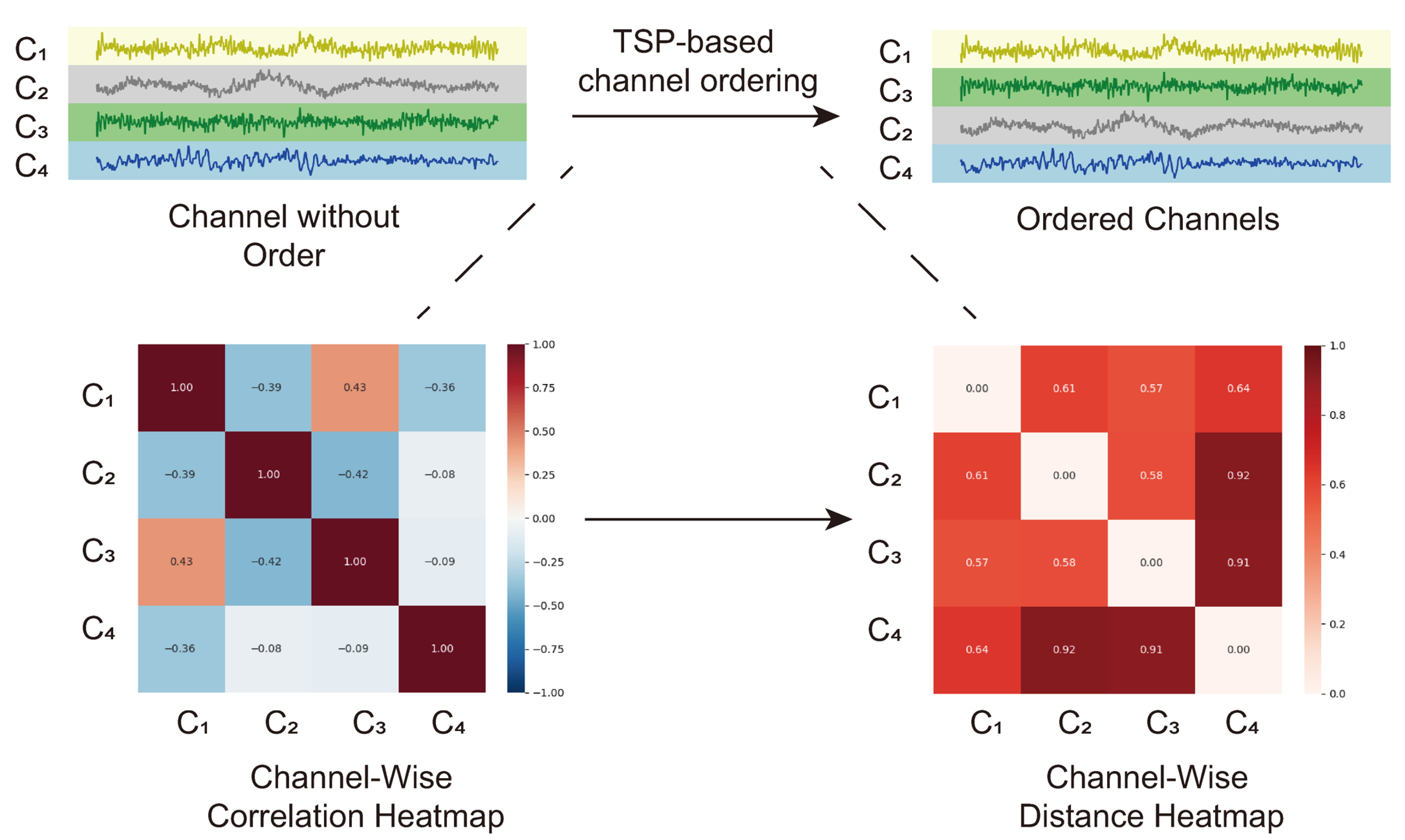
- It is shown that the overall prediction accuracy can be improved by reordering the channels, so that more correlated channels are put closer together. The channel reordering is formulated as the TSP. Since solving the TSP is computationally expensive, only the channels of the weakest UPs are reordered, and the corresponding predictors are retrained. Such a two-stage training extends other existing methods proposed in the literature.
- The improvements in the prediction accuracy due to the designed 2D symbol-EMD front-end with channel reordering are demonstrated numerically using a bank of the most common UPs, including DLinear, FITS, and TCN, respectively.
2. Data Processing Modules
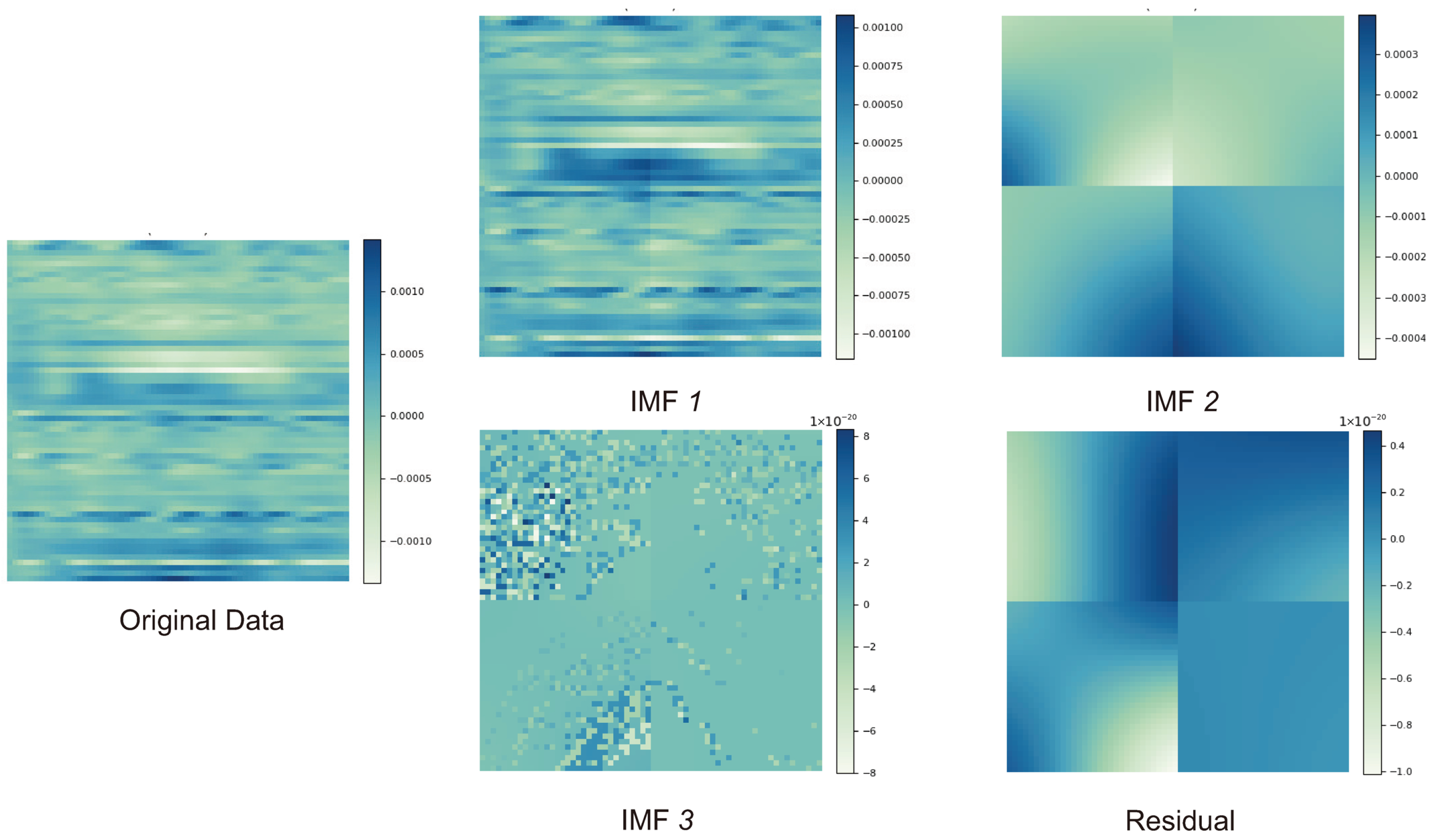
2.1. A 2D-EMD Module
- Input normalization: The input samples are transformed to using the min–max normalization, i.e.,The normalization ensures consistent properties across space and time for extrema detection and envelope interpolation.
- Boundary extension: The normalized symbols are extended to using mirror-padding reflecting their values along the horizontal and vertical directions. This creates larger matrices in which the original samples are surrounded by their mirrored copies. It improves the accuracy of extrema detection near the original symbol boundaries, which yields smoother and more consistent IMF components.
- Extrema detection: The local maxima and minima, and , respectively, within the symbol are identified by comparing the samples with their neighboring values using a sliding 2D window. The extrema detection can be repeated multiple times in order to improve the robustness.
- Envelope construction: The extrema are interpolated in order to construct the upper and lower envelopes, and , respectively, using the bivariate splines , i.e.,
- Mean removal: The mean envelope is computed and subtracted, i.e.,The resulting symbol becomes the candidate IMF after one sifting iteration.
- The IMF criterion check: Steps 3–5 are performed repeatedly until the IMF condition is satisfied. In such a case, satisfying the IMF condition becomes the i-th IMF component, .
- Residual update and decomposition loops: The extracted IMF components are subtracted from the current residual until the remaining residual have no significant oscillatory modes, and the sifting process of extracting the IMF components can be terminated.
- Inverse (re-)normalization: At the final step, all extracted IMF components are re-normalized using an inverse min–max normalization in order to restore the scale of the original data samples.
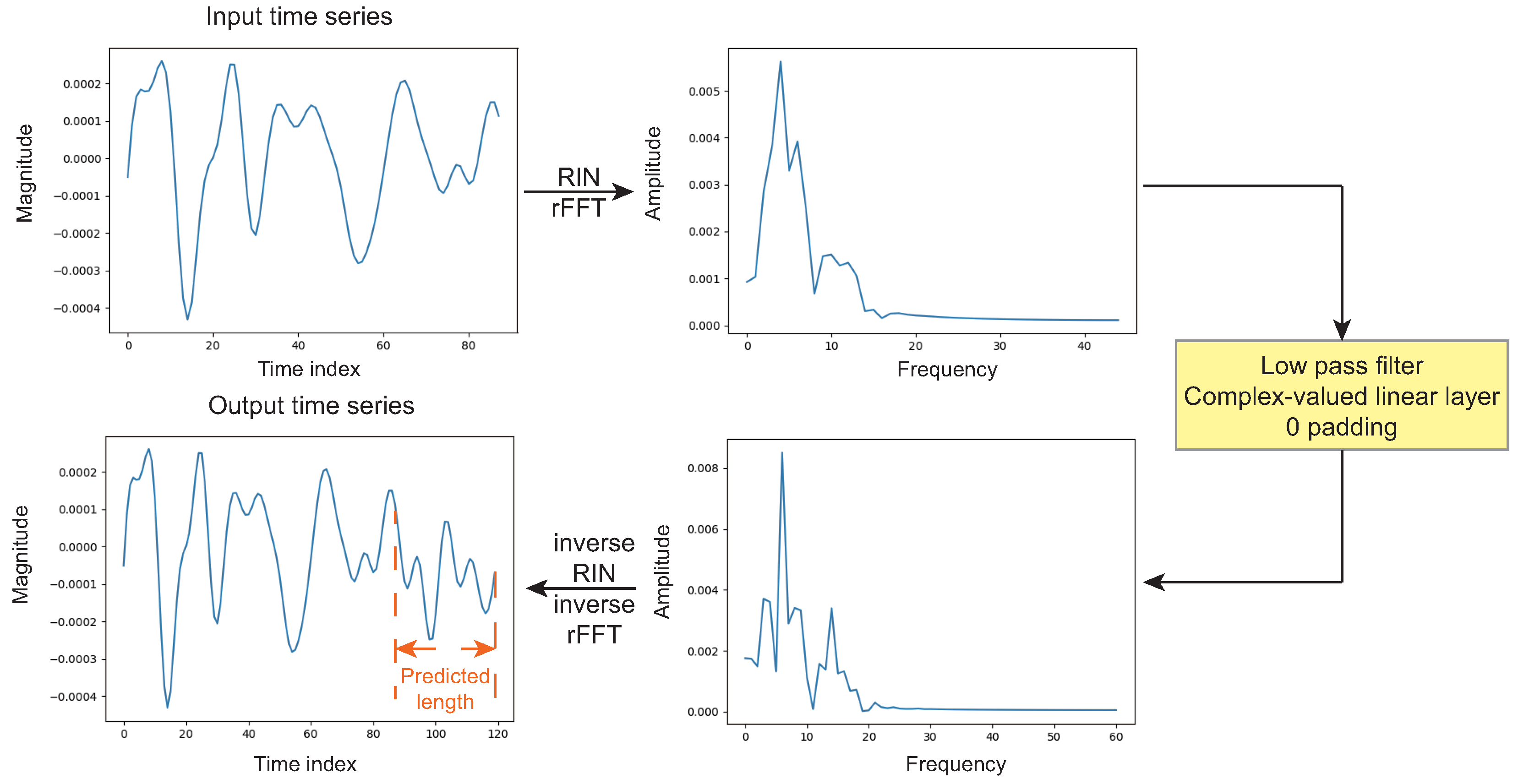
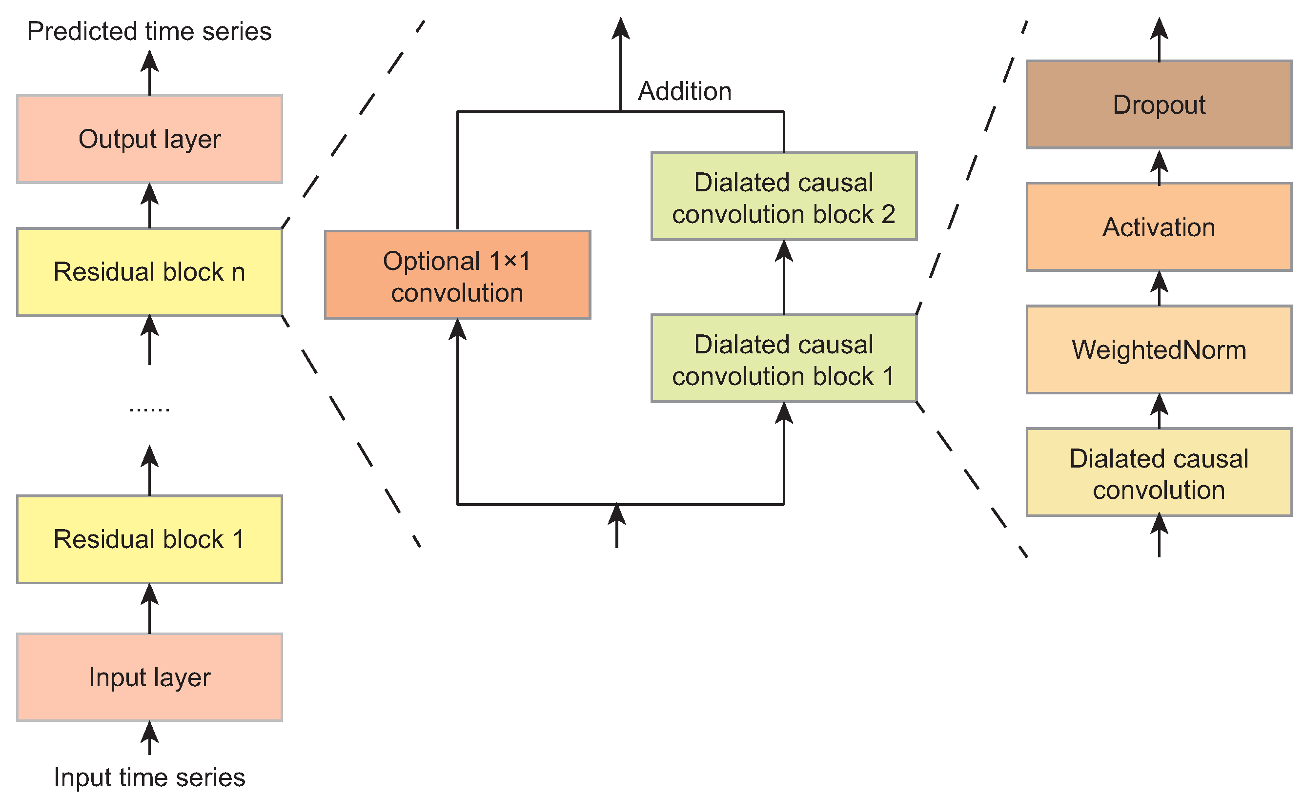
2.2. UP Modules
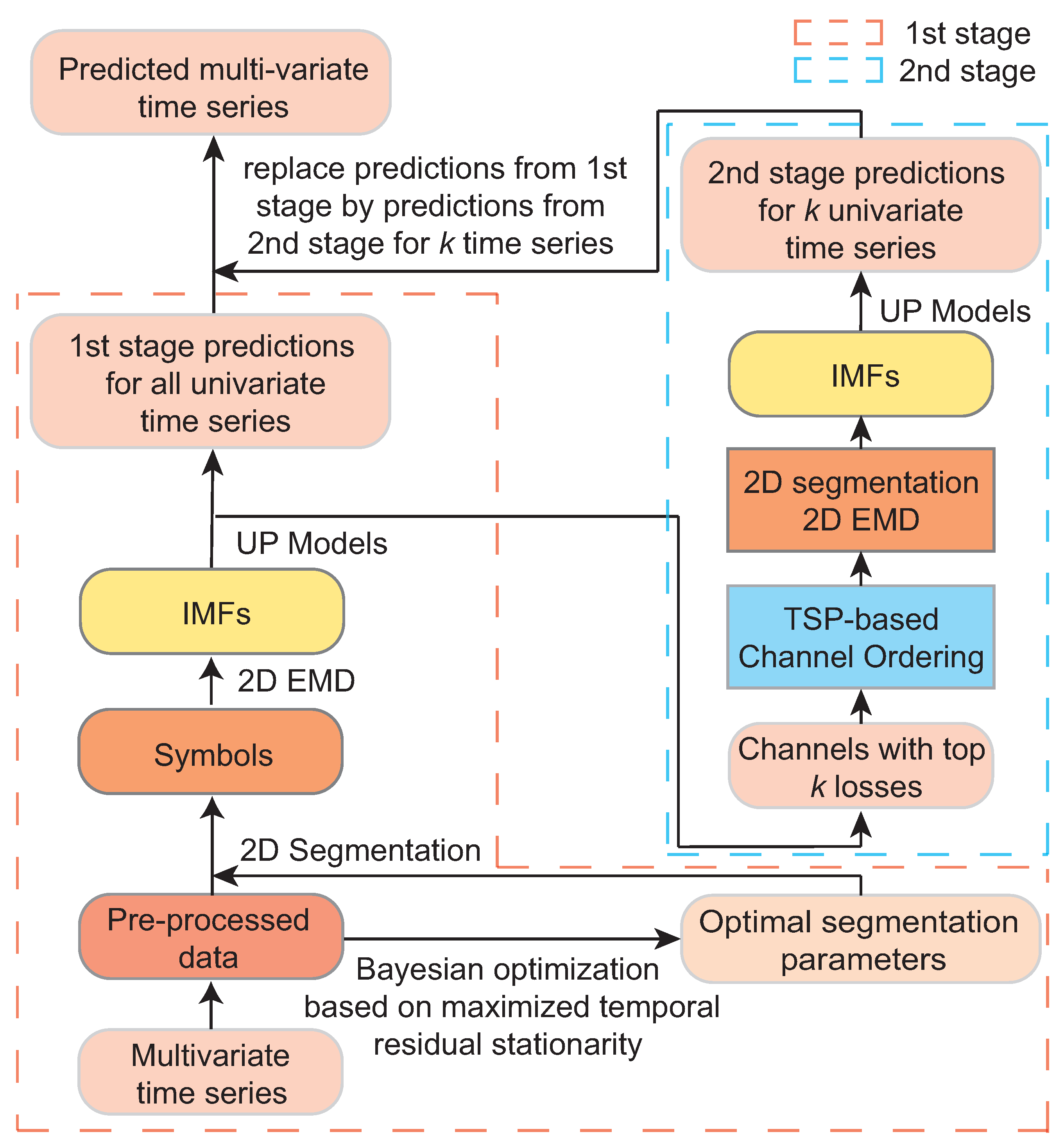
3. A Two-Stage Symbol-EMD-UP
3.1. TSP-Based Channel Reordering
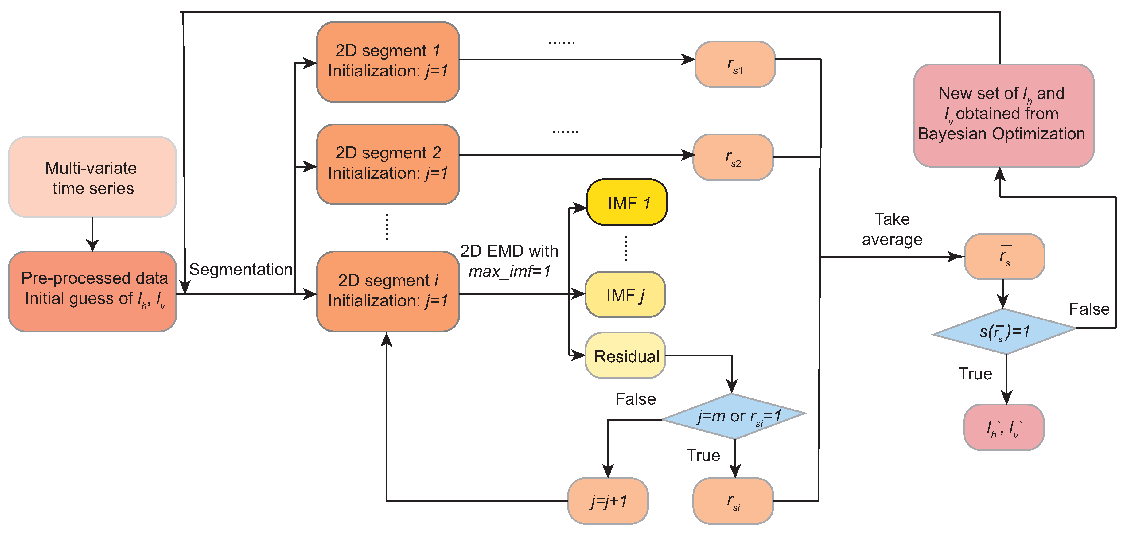
3.2. The Overall Architecture
4. Numerical Experiments
4.1. Evaluation Metrics
4.2. Experimental Setting
4.3. Comparison of Forecasting Accuracy of Different Systems
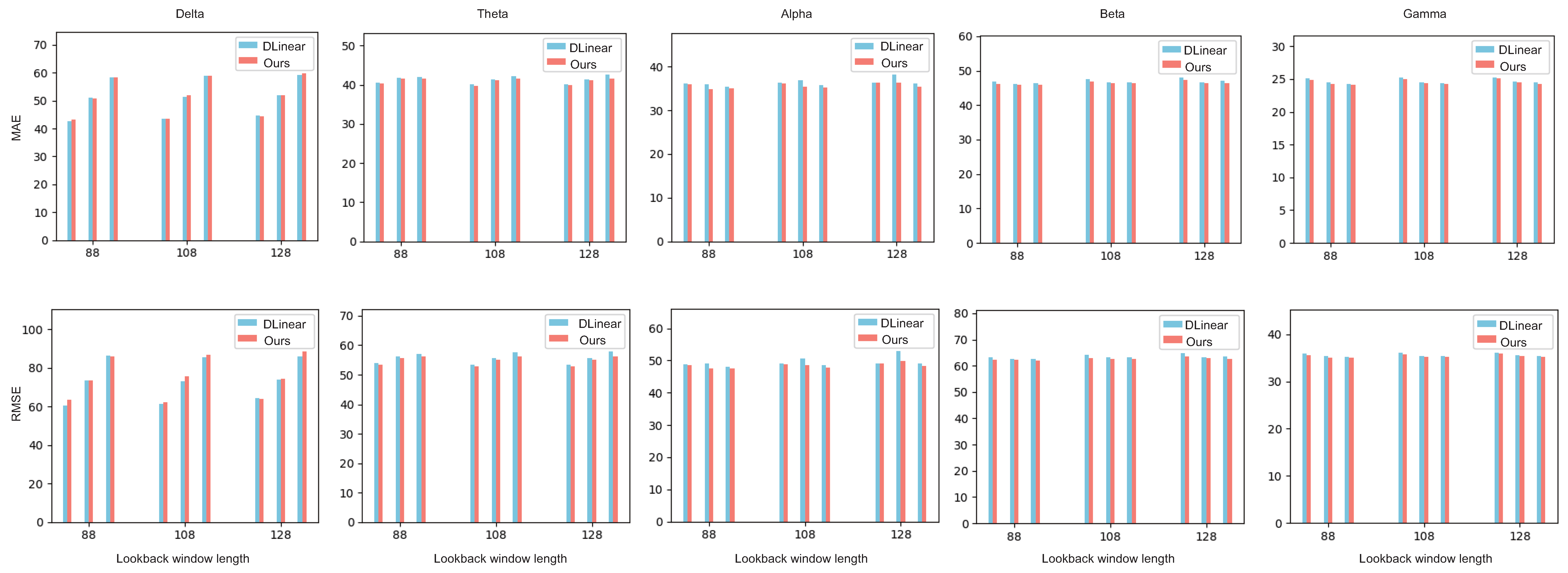
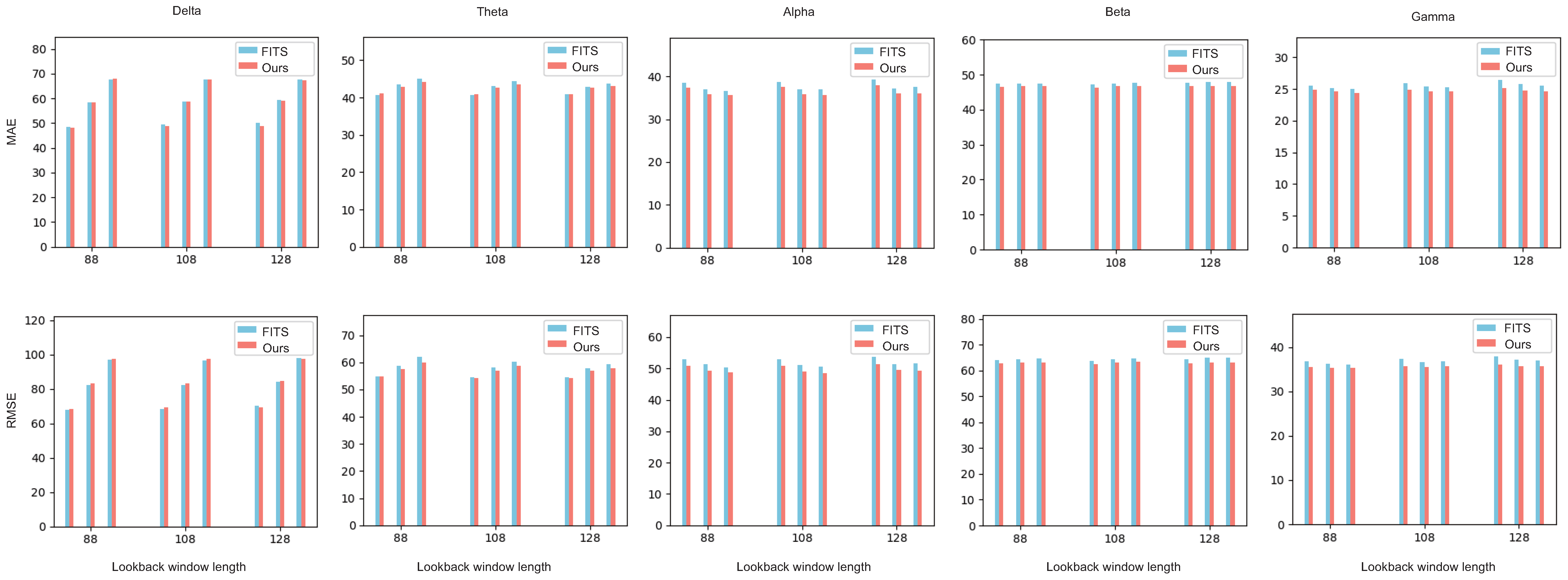
4.4. Forecasting Accuracy in Different Frequency Bands
4.5. Impact of Channel Reordering on Forecasting Accuracy
5. Conclusions
Author Contributions
Funding
Data Availability Statement
Conflicts of Interest
References
- Cho, H.; Ahn, M.; Ahn, S.; Kwon, M.; Jun, S. EEG Datasets for Motor Imagery Brain Computer Interface. GigaScience 2017, 6, gix034. [Google Scholar] [CrossRef]
- Pankka, H.; Lehtinen, J.; Ilmoniemi, R.J.; Roine, T. Enhanced EEG Forecasting: A Probabilistic Deep Learning Approach. Neural Comput. 2025, 37, 793–814. [Google Scholar] [CrossRef] [PubMed]
- Diebold, F.X. Elements of Forecasting, 4th ed.; Thomson South-Western: Mason, OH, USA, 2006. [Google Scholar]
- Zhou, H.; Zhang, S.; Peng, J.; Zhang, S.; Li, J.; Xiong, H.; Zhang, W. Informer: Beyond Efficient Transformer for Long Sequence Time-Series Forecasting. Proc. AAAI 2021, 35, 11106–11115. [Google Scholar] [CrossRef]
- Wu, H.; Xu, J.; Wang, J.; Long, M. Autoformer: Decomposition Transformers with Auto-Correlation for Long-Term Series Forecasting. Proc. NeurIPS 2021, 34, 22419–22430. [Google Scholar]
- Zeng, A.; Chen, M.; Zhang, L.; Xu, Q. Are Transformers Effective for Time Series Forecasting? Proc. AAAI 2023, 1248, 11121–11128. [Google Scholar] [CrossRef]
- Zhang, T.; Zhang, Y.; Cao, W.; Bian, J.; Yi, X.; Zheng, S.; Li, J. Less Is More: Fast Multivariate Time Series Forecasting with Light Sampling-oriented MLP Structures. arXiv 2022, arXiv:2207.01186. [Google Scholar]
- Das, A.; Kong, W.; Leach, A.; Mathur, S.K.; Sen, R.; Yu, R. Long-Term Forecasting with TIDE: Time-Series Dense Encoder. arXiv 2023, arXiv:2304.08424. [Google Scholar]
- Lin, S.; Lin, W.; Wu, W.; Chen, H.; Yang, J. SparseTSF: Modeling Long-Term Time Series Forecasting with 1K Parameters. In Proceedings of the 41st ICML, Vienna, Austria, 21–27 July 2024. [Google Scholar]
- Han, L.; Ye, H.J.; Zhan, D.C. The Capacity and Robustness Trade-Off: Revisiting the Channel Independent Strategy for Multivariate Time Series Forecasting. IEEE Trans. Knowl. Data Eng. 2024, 36, 7129–7142. [Google Scholar] [CrossRef]
- Elsayed, S.; Thyssens, D.; Rashed, A.; Jomaa, H.S.; Schmidt-Thieme, L. Do We Really Need Deep Learning Models for Time Series Forecasting? arXiv 2021, arXiv:2101.02118. [Google Scholar]
- Ekambaram, V.; Jati, A.; Nguyen, N.; Sinthong, P.; Kalagnanam, J. TSMixer: Lightweight MLP-Mixer Model for Multivariate Time Series Forecasting. In Proceedings of the 29th ACM CKDDM, Long Beach, CA, USA, 6–10 August 2023; pp. 459–469. [Google Scholar]
- Xu, Z.; Zeng, A.; Xu, Q. FITS: Modeling Time Series with 10K Parameters. In Proceedings of the 12th ICLR, Vienna, Austria, 7–11 May 2024. [Google Scholar]
- Duarte, F.S.; Rios, R.A.; Hruschka, E.R.; de Mello, R.F. Decomposing Time Series Into Deterministic and Stochastic Influences: A Survey. Digit. Signal Process. 2019, 95, 102582. [Google Scholar] [CrossRef]
- Golyandina, N.; Nekrutkin, V.; Zhigljavsky, A.A. Analysis of Time Series Structure: SSA and Related Techniques; CRC Press: Boca Raton, FL, USA, 2001. [Google Scholar]
- Shumway, R.H.; Stoffer, D.S. Time Series Analysis and Its Applications; Springer: Berlin/Heidelberg, Germany, 2000; Volume 3. [Google Scholar]
- Huang, N.E.; Shen, Z.; Long, S.R.; Wu, M.C.; Shih, H.H.; Zheng, Q.; Yen, N.C.; Tung, C.C.; Liu, H.H. The Empirical Mode Decomposition and the Hilbert Spectrum for Nonlinear and Non-stationary Time Series Analysis. Proc. R. Soc. Lond. Ser. A 1998, 454, 903–995. [Google Scholar] [CrossRef]
- Huang, S.; Chang, J.; Huang, Q.; Chen, Y. Monthly Streamflow Prediction Using Modified EMD-Based Support Vector Machine. J. Hydrol. 2014, 511, 764–775. [Google Scholar] [CrossRef]
- Niu, W.; Feng, Z.; Chen, Y.; Zhang, H.; Cheng, C. Annual Streamflow Time Series Prediction Using Extreme Learning Machine Based on Gravitational Search Algorithm and Variational Mode Decomposition. J. Hydrol. Eng. 2020, 25, 04020008. [Google Scholar] [CrossRef]
- Feng, Z.; Niu, W.; Wan, X.; Xu, B.; Zhu, F.; Chen, J. Hydrological Time Series Forecasting via Signal Decomposition and Twin Support Vector Machine Using Cooperation Search Algorithm for Parameter Identification. J. Hydrol. 2022, 612, 128213. [Google Scholar] [CrossRef]
- Wen, X.; Feng, Q.; Deo, R.C.; Wu, M.; Yin, Z.; Yang, L.; Singh, V.P. Two-Phase Extreme Learning Machines Integrated with the Complete Ensemble Empirical Mode Decomposition with Adaptive Noise Algorithm for Multi-Scale Runoff Prediction Problems. J. Hydrol. 2019, 570, 167–184. [Google Scholar] [CrossRef]
- Wang, L.; Li, X.; Ma, C.; Bai, Y. Improving the Prediction Accuracy of Monthly Streamflow Using a Data-Driven Model Based on a Double-Processing Strategy. J. Hydrol. 2019, 573, 733–745. [Google Scholar] [CrossRef]
- Wang, W.; Cheng, Q.; Chau, K.; Hu, H.; Zang, H.; Xu, D.M. An Enhanced Monthly Runoff Time Series Prediction Using Extreme Learning Machine Optimized by Salp Swarm Algorithm Based on Time Varying Filtering Based Empirical Mode Decomposition. J. Hydrol. 2023, 620, 129460. [Google Scholar] [CrossRef]
- Abbasimehr, H.; Behboodi, A.; Bahrini, A. A novel hybrid model to forecast seasonal and chaotic time series. Expert Syst. Appl. 2024, 239, 122461. [Google Scholar] [CrossRef]
- Fan, G.; Wei, H.; Huang, H.; Hong, W. Application of ensemble empirical mode decomposition with support vector regression and wavelet neural network in electric load forecasting. Energy Sources Part B Econ. Plan. Policy 2025, 20, 2468687. [Google Scholar] [CrossRef]
- Zhong, B.; Yang, L.; Li, B.; Ji, M. Short-term power grid load forecasting based on VMD-SE-Bilstm-Attention hybrid model. Int. J.-Low-Carbon Technol. 2024, 19, 1951–1958. [Google Scholar] [CrossRef]
- Wu, B.; Wang, L. Two-stage decomposition and temporal fusion transformers for interpretable wind speed forecasting. Energy 2024, 288, 129728. [Google Scholar] [CrossRef]
- Liang, P.; Zhang, Y.; Ding, Y.; Chen, J.; Madukoma, C.S.; Weninger, T.; Shrout, J.D.; Chen, D.Z. H-EMD: A Hierarchical Earth Mover’s Distance Method for Instance Segmentation. IEEE Trans. Med. Imaging 2022, 41, 2582–2597. [Google Scholar] [CrossRef]
- Yang, L.; Lu, F.; Zhang, T.; Chen, J. Texture Feature Extraction of Image Based on 2D Hilbert-Huang Transform and Multifractal Analysis. In Proceedings of the ICICML, Chengdu, China, 3–5 November 2023; pp. 57–63. [Google Scholar] [CrossRef]
- Ma, P.; Ren, J.; Sun, G.; Zhao, H.; Jia, X.; Yan, Y.; Zabalza, J. Multiscale Superpixelwise Prophet Model for Noise-Robust Feature Extraction in Hyperspectral Images. IEEE Trans. Geosci. Remote Sens. 2023, 61, 1–12. [Google Scholar] [CrossRef]
- Zhu, H.; Sun, R.; Xu, Z.; Lv, C.; Bi, R. Prediction of Soil Nutrients Based on Topographic Factors and Remote Sensing Index in a Coal Mining Area, China. Sustainability 2020, 12, 1626. [Google Scholar] [CrossRef]
- Bai, S.; Kolter, J.Z.; Koltun, V. An Empirical Evaluation of Generic Convolutional and Recurrent Networks for Sequence Modeling. arXiv 2018, arXiv:1803.01271. [Google Scholar]
- Dickey, D.A. 192-30: Stationarity Issues in Time Series Models. In Proceedings of the SUGI 30, Philadelphia, PA, USA, 10–13 April 2005; pp. 1–17. [Google Scholar]
- Yu, Y.; Loskot, P.; Zhang, W.; Zhang, Q.; Gao, Y. Joint Multivariate Time Series Forecasting Using Empirical Symbol Mode Decomposition Modeling. In Proceedings of the ICCCM, Okinawa, Japan, 11–13 July 2025; pp. 1–10. [Google Scholar]
- Koh, M.S.; Rodriguez-Marek, E.; Fischer, T.R. A New Two Dimensional Empirical Mode Decomposition for Images Using Inpainting. In Proceedings of the 10th ICSP, Beijing, China, 24–28 October 2010; pp. 13–16. [Google Scholar] [CrossRef]
- Laszuk, D. Python Implementation of Empirical Mode Decomposition Algorithm. GitHub Repository. 2017. Available online: https://github.com/laszukdawid/PyEMD (accessed on 5 July 2025).
- Déaz-Rós, D.; Salazar-González, J.J. Mathematical Formulations for Consistent Travelling Salesman Problems. Eur. J. Oper. Res. 2024, 313, 465–477. [Google Scholar] [CrossRef]
- Aggarwal, S.; Chugh, N. Review of Machine Learning Techniques for EEG Based Brain Computer Interface. Arch. Comput. Methods Eng. 2022, 29, 3001–3020. [Google Scholar] [CrossRef]


| System | Parameter | Value |
|---|---|---|
| Symbol-EMD | [32, 1024] | |
| {16, 32, 64} | ||
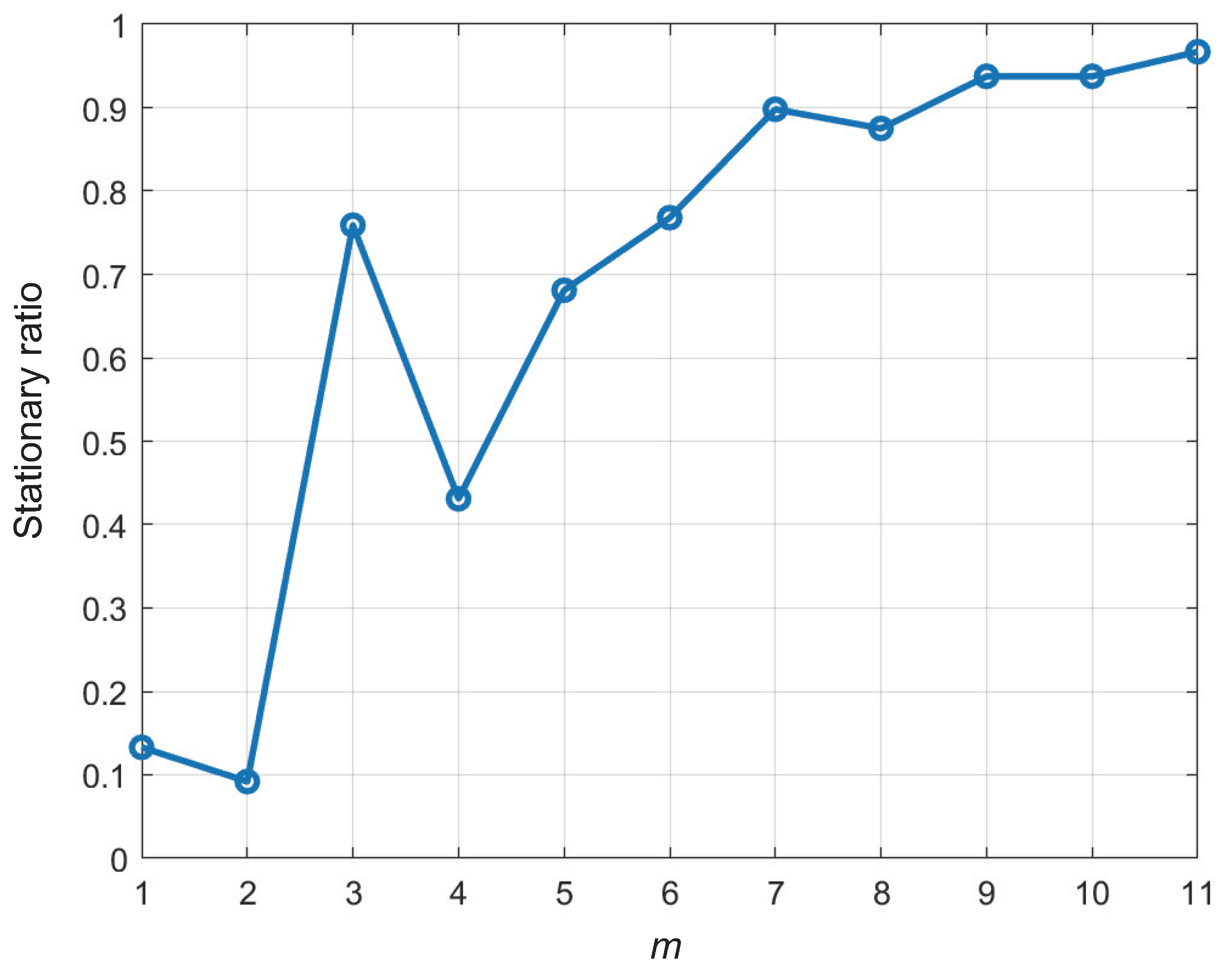
| m | 3 | |
| All UP predictions | Look-back window | {88, 108, 128} |
| Prediction horizon | {32, 48, 64} | |
| DLinear | Batch size | 32 |
| FITS | Batch size | 32 |
| LPF cut-off freq. | 40 Hz | |
| TCN | Batch size | 16 |
| Number of layers | 4 | |
| Dropout | 0.2 | |
| Ordering | k | 4 |
| Look-Back | Horizon | DLinear | EMD-DLinear | Symbol-EMD- DLinear | Two-Stage Symbol-EMD-DLinear with Ordering | ||||
|---|---|---|---|---|---|---|---|---|---|
| MAE | RMSE | MAE | RMSE | MAE | RMSE | MAE | RMSE | ||
| 88 | 32 | 106.63 | 146.77 | 106.20 | 146.96 | 105.60 | 146.54 | 105.13 | 145.62 |
| 48 | 112.26 | 154.64 | 111.49 | 153.85 | 110.70 | 152.99 | 110.10 | 151.67 | |
| 64 | 117.83 | 163.58 | 116.92 | 162.32 | 116.09 | 161.26 | 115.58 | 160.18 | |
| 108 | 32 | 108.13 | 148.35 | 107.55 | 147.71 | 106.90 | 147.29 | 106.36 | 146.22 |
| 48 | 113.68 | 155.86 | 112.99 | 154.99 | 112.37 | 155.28 | 111.72 | 153.98 | |
| 64 | 119.83 | 165.24 | 118.95 | 164.67 | 117.91 | 163.49 | 117.29 | 162.20 | |
| 128 | 32 | 109.46 | 150.29 | 108.43 | 148.77 | 107.66 | 147.80 | 107.48 | 147.84 |
| 48 | 115.07 | 157.38 | 114.43 | 156.72 | 113.57 | 155.75 | 112.97 | 154.71 | |
| 64 | 121.12 | 166.98 | 120.52 | 166.38 | 119.32 | 165.06 | 118.73 | 164.21 | |
| Look-Back | Horizon | FITS | EMD-FITS | Symbol-EMD- FITS | Two-Stage Symbol-EMD-FITS with Ordering | ||||
|---|---|---|---|---|---|---|---|---|---|
| MAE | RMSE | MAE | RMSE | MAE | RMSE | MAE | RMSE | ||
| 88 | 32 | 108.65 | 150.74 | 108.34 | 149.38 | 107.04 | 147.85 | 106.86 | 147.62 |
| 48 | 115.33 | 159.06 | 114.79 | 157.83 | 113.76 | 156.80 | 113.60 | 156.62 | |
| 64 | 122.04 | 169.30 | 121.65 | 168.17 | 120.70 | 166.94 | 120.62 | 166.70 | |
| 108 | 32 | 109.26 | 150.65 | 108.68 | 149.48 | 107.30 | 147.87 | 107.24 | 148.01 |
| 48 | 115.57 | 159.08 | 114.80 | 157.60 | 113.67 | 156.20 | 113.64 | 156.24 | |
| 64 | 122.20 | 169.27 | 121.50 | 167.76 | 120.48 | 166.45 | 120.48 | 166.39 | |
| 128 | 32 | 110.63 | 152.54 | 109.44 | 150.37 | 107.96 | 148.57 | 107.82 | 148.42 |
| 48 | 116.43 | 160.12 | 115.51 | 158.31 | 114.39 | 156.94 | 114.35 | 157.10 | |
| 64 | 122.54 | 169.75 | 121.76 | 168.01 | 120.67 | 166.53 | 120.62 | 166.36 | |
| Look-Back | Horizon | TCN | EMD-TCN | Symbol-EMD- TCN | Two-Stage Symbol-EMD-TCN with Ordering | ||||
|---|---|---|---|---|---|---|---|---|---|
| MAE | RMSE | MAE | RMSE | MAE | RMSE | MAE | RMSE | ||
| 88 | 32 | 101.71 | 143.12 | 103.91 | 147.96 | 101.75 | 144.22 | 98.37 | 136.75 |
| 48 | 106.73 | 148.12 | 106.79 | 148.11 | 106.80 | 148.50 | 103.81 | 144.60 | |
| 64 | 111.68 | 155.67 | 111.79 | 155.99 | 111.85 | 157.09 | 108.74 | 155.88 | |
| 108 | 32 | 102.02 | 143.98 | 103.70 | 145.38 | 101.95 | 144.39 | 98.67 | 137.41 |
| 48 | 107.04 | 150.18 | 107.00 | 147.97 | 107.10 | 149.92 | 103.61 | 142.61 | |
| 64 | 111.87 | 156.26 | 112.53 | 161.34 | 112.05 | 157.29 | 109.02 | 154.60 | |
| 128 | 32 | 102.43 | 148.39 | 104.14 | 147.87 | 102.26 | 143.83 | 99.13 | 138.54 |
| 48 | 107.11 | 148.94 | 107.07 | 148.16 | 106.95 | 148.63 | 103.94 | 145.09 | |
| 64 | 112.50 | 158.60 | 112.30 | 157.27 | 112.53 | 159.34 | 109.85 | 158.81 | |
| Look-Back | Horizon | Two-Stage Symbol-EMD-DLinear with Ordering | Two-Stage Symbol-EMD-FITS with Ordering | Two-Stage Symbol-EMD-TCN with Ordering | |||
|---|---|---|---|---|---|---|---|
| MAERR | RMSERR | MAERR | RMSERR | MAERR | RMSERR | ||
| 88 | 32 | 1.41 | 0.78 | 1.65 | 2.07 | 3.29 | 4.45 |
| 48 | 1.92 | 1.92 | 1.50 | 1.53 | 2.74 | 2.38 | |
| 64 | 1.91 | 2.08 | 1.16 | 1.54 | 2.63 | −0.13 | |
| 108 | 32 | 1.68 | 1.44 | 1.85 | 1.75 | 3.29 | 4.56 |
| 48 | 1.72 | 1.20 | 1.67 | 1.79 | 3.20 | 5.04 | |
| 64 | 2.12 | 1.840 | 1.41 | 1.70 | 2.54 | 1.07 | |
| 128 | 32 | 1.81 | 1.629 | 2.54 | 2.705 | 3.22 | 6.64 |
| 48 | 1.83 | 1.69 | 1.78 | 1.884 | 2.96 | 2.58 | |
| 64 | 1.97 | 1.66 | 1.57 | 2.00 | 2.36 | −0.13 | |
| Average | 1.81 | 1.58 | 1.68 | 1.89 | 2.91 | 2.94 | |
| Wave Bands | Symbol-EMD-DLinear with Ordering | Symbol-EMD-FITS with Ordering | Symbol-EMD-TCN with Ordering | |||
|---|---|---|---|---|---|---|
| MAERR | RMSERR | MAERR | RMSERR | MAERR | RMSERR | |
| Delta | −0.29 | −1.61 | 0.52 | −0.46 | 1.20 | 1.20 |
| Theta | 1.06 | 1.41 | 0.79 | 1.59 | 1.6 | 0.76 |
| Alpha | 1.87 | 2.08 | 3.24 | 3.97 | 2.4 | 2.78 |
| Beta | 1.05 | 1.14 | 1.93 | 2.26 | 2.92 | 3.71 |
| Gamma | 0.69 | 0.68 | 3.28 | 3.52 | 4.90 | 7.51 |
| Look-Back | Horizon | MCCMA Ordered | LCCMA Ordered | Not Ordered | |||
|---|---|---|---|---|---|---|---|
| MAERR | RMSERR | MAERR | RMSERR | MAERR | RMSERR | ||
| 88 | 32 | 1.41 | 0.78 | 1.11 | 0.60 | 0.85 | −0.13 |
| 48 | 1.92 | 1.92 | 1.61 | 1.29 | 1.51 | 1.02 | |
| 64 | 1.91 | 2.08 | 1.42 | 1.09 | 1.48 | 1.37 | |
| 108 | 32 | 1.64 | 1.44 | 1.77 | 2.10 | 1.71 | 2.01 |
| 48 | 1.72 | 1.20 | 1.77 | 2.13 | 1.72 | 1.90 | |
| 64 | 2.12 | 1.84 | 1.96 | 1.94 | 2.00 | 1.98 | |
| 128 | 32 | 1.81 | 1.63 | 1.37 | 0.78 | 1.36 | 1.18 |
| 48 | 1.82 | 1.69 | 1.81 | 2.03 | 1.70 | 1.87 | |
| 64 | 1.97 | 1.66 | 2.12 | 2.27 | 2.16 | 2.26 | |
| Average | 1.81 | 1.58 | 1.66 | 1.58 | 1.61 | 1.50 | |
| Look-Back | Horizon | MCCMA Ordered | LCCMA Ordered | Not Ordered | |||
|---|---|---|---|---|---|---|---|
| MAERR | RMSERR | MAERR | RMSERR | MAERR | RMSERR | ||
| 88 | 32 | 1.65 | 2.07 | 1.26 | 1.10 | 1.30 | 1.21 |
| 48 | 1.50 | 1.53 | 1.36 | 0.87 | 1.41 | 0.94 | |
| 64 | 1.16 | 1.54 | 1.12 | 1.32 | 1.11 | 1.33 | |
| 108 | 32 | 1.85 | 1.75 | 1.42 | 0.65 | 1.54 | 0.95 |
| 48 | 1.67 | 1.79 | 1.51 | 1.17 | 1.50 | 1.13 | |
| 64 | 1.41 | 1.70 | 1.36 | 1.49 | 1.42 | 1.53 | |
| 128 | 32 | 2.54 | 2.70 | 2.11 | 1.66 | 2.21 | 1.88 |
| 48 | 1.78 | 1.88 | 1.51 | 1.14 | 1.54 | 1.15 | |
| 64 | 1.57 | 2.00 | 1.51 | 1.79 | 1.61 | 1.98 | |
| Average | 1.68 | 1.89 | 1.46 | 1.24 | 1.51 | 1.34 | |
| Look-Back | Horizon | MCCMA Ordered | LCCMA Ordered | Not Ordered | |||
|---|---|---|---|---|---|---|---|
| MAERR | RMSERR | MAERR | RMSERR | MAERR | RMSERR | ||
| 88 | 32 | 3.29 | 4.45 | 3.30 | 4.95 | 3.04 | 2.99 |
| 48 | 2.74 | 2.38 | 2.51 | 1.94 | 2.77 | 3.56 | |
| 64 | 2.63 | −0.13 | 2.87 | 2.55 | 2.87 | 2.09 | |
| 108 | 32 | 3.29 | 4.56 | 2.73 | −0.39 | 3.01 | 3.84 |
| 48 | 3.20 | 5.04 | 2.65 | 1.58 | 2.97 | 3.20 | |
| 64 | 2.54 | 1.07 | 2.65 | −2.54 | 2.41 | −0.94 | |
| 128 | 32 | 3.22 | 6.64 | 3.12 | 6.44 | 2.53 | −0.03 |
| 48 | 2.96 | 2.58 | 2.76 | 2.25 | 2.68 | −1.54 | |
| 64 | 2.35 | −0.13 | 2.77 | 2.49 | 2.25 | 2.19 | |
| Average | 2.91 | 2.94 | 2.82 | 2.14 | 2.73 | 1.71 | |
Disclaimer/Publisher’s Note: The statements, opinions and data contained in all publications are solely those of the individual author(s) and contributor(s) and not of MDPI and/or the editor(s). MDPI and/or the editor(s) disclaim responsibility for any injury to people or property resulting from any ideas, methods, instructions or products referred to in the content. |
© 2025 by the authors. Licensee MDPI, Basel, Switzerland. This article is an open access article distributed under the terms and conditions of the Creative Commons Attribution (CC BY) license (https://creativecommons.org/licenses/by/4.0/).
Share and Cite
Yu, Y.; Loskot, P.; Zhang, W.; Zhang, Q.; Gao, Y. A Spatial–Temporal Time Series Decomposition for Improving Independent Channel Forecasting. Mathematics 2025, 13, 2221. https://doi.org/10.3390/math13142221
Yu Y, Loskot P, Zhang W, Zhang Q, Gao Y. A Spatial–Temporal Time Series Decomposition for Improving Independent Channel Forecasting. Mathematics. 2025; 13(14):2221. https://doi.org/10.3390/math13142221
Chicago/Turabian StyleYu, Yue, Pavel Loskot, Wenbin Zhang, Qi Zhang, and Yu Gao. 2025. "A Spatial–Temporal Time Series Decomposition for Improving Independent Channel Forecasting" Mathematics 13, no. 14: 2221. https://doi.org/10.3390/math13142221
APA StyleYu, Y., Loskot, P., Zhang, W., Zhang, Q., & Gao, Y. (2025). A Spatial–Temporal Time Series Decomposition for Improving Independent Channel Forecasting. Mathematics, 13(14), 2221. https://doi.org/10.3390/math13142221