Variational Bayesian Variable Selection in Logistic Regression Based on Spike-and-Slab Lasso

Abstract

Logistic regression is often used to solve classification problems. This article combines the advantages of Bayesian methods and spike-and-slab Lasso to select variables in high-dimensional logistic regression. The method of introducing a new hidden variable or approximating the lower bound is used to solve the problem of logistic functions without conjugate priors. The Laplace distribution in spike-and-slab Lasso is expressed as a hierarchical form of normal distribution and exponential distribution, so that all parameters in the model are posterior distributions that are easy to deal with. Considering the high time cost of parameter estimation and variable selection in high-dimensional models, we use the variational Bayesian algorithm to perform posterior inference on the parameters in the model. From the simulation results, it can be seen that it is an adaptive prior that can perform parameter estimation and variable selection well in high-dimensional logistic regression. From the perspective of algorithm running time, the method proposed in this article also has high computational efficiency in many cases.

1. Introduction

Logistic regression is widely used for classification problems and remains a popular model among statisticians and machine learning researchers [1]. Let $X\in {\mathbb{R}}^{p+1}$ denote the $(p+1)$-dimensional covariate vector, where the first element of X is set to 1, and let $y\in \{0,1\}$ be the binary response. Suppose we observe n pairs of data $(X_i,y_i)$ for $i=1,\dots ,n$, the standard form of the logistic regression model is:

$$P\left(y_i=1\mid X_i\right)=1-P\left(y_i=0\mid X_i\right)=\sigma \left(X_i^T\mathit{\beta }\right)={\displaystyle \frac{e^{X_i^T\mathit{\beta }}}{1+e^{X_i^T\mathit{\beta }}}},$$

(1)

where $\mathit{\beta }=({\beta }_0,{\beta }_1,\dots ,{\beta }_p)\in {\mathbb{R}}^{p+1}$ denotes the regression coefficients, ${\beta }_0$ is the intercept term, and $\sigma \left(t\right)=e^t/(1+e^t)$ is the logistic function.

With the advent of the “big data era,” high-dimensional sparsity has become a common assumption in regression modeling. In settings where $p>n$ or even $p\gg n$, variable selection is essential for identifying simpler models in which most regression coefficients are zero (or near zero). This not only enhances model interpretability but also mitigates overfitting and multicollinearity.

Variable selection approaches can be broadly grouped into three categories: (1) Traditional methods based on significance testing or information criteria (e.g., AIC, BIC); (2) Penalization-based approaches that perform selection via regularization, such as the LASSO (Least Absolute Shrinkage and Selection Operator) [2], Smoothly Clipped Absolute Deviation (SCAD) [3], and the Minimax Concave Penalty (MCP) [4]; (3) Bayesian methods that induce sparsity through shrinkage priors, including continuous shrinkage priors and two-component mixture priors such as the spike-and-slab prior.

Among these, significance-based and information-theoretic approaches are increasingly seen as unreliable in high-dimensional settings or in the presence of multicollinearity. Penalization-based methods like the LASSO have gained widespread popularity, and many such methods can be reinterpreted within a Bayesian framework by specifying appropriate priors. In fact, Bayesian variable selection has been shown—both theoretically and empirically—to perform on par with or even outperform frequentist approaches [5,6,7]. Consequently, this work adopts the Bayesian paradigm for variable selection.

While Bayesian shrinkage priors do not perform variable selection in a strict sense, practitioners often apply thresholding rules on posterior estimates to identify important variables—that is, variables are retained if their posterior mean or inclusion probability exceeds a certain threshold. Although widely used, the theoretical properties of such thresholding procedures remain underexplored.

Variable selection can also be viewed as a special case of model selection. A popular Bayesian prior for this purpose is the spike-and-slab prior, expressed as:

$${\beta }_j\mid {\gamma }_j\sim {\gamma }_j{\phi }_1\left({\beta }_j\right)+(1-{\gamma }_j){\phi }_0\left({\beta }_j\right),j=1,2,\dots ,p,$$

(2)

where ${\phi }_1\left({\beta }_j\right)$ is typically a diffuse distribution (“slab”) modeling large coefficients, and ${\phi }_0\left({\beta }_j\right)$ is a concentrated distribution (“spike”) capturing small or null coefficients. The binary indicator ${\gamma }_j$ determines whether the j-th variable is included (${\gamma }_j=1$) or excluded (${\gamma }_j=0$). The spike-and-slab prior therefore provides an explicit mechanism for variable selection, with ${\gamma }_j$ serving as a measure of variable importance.

A well-known formulation is the Stochastic Search Variable Selection (SSVS) prior by George and McCulloch [8], where both ${\phi }_1$ and ${\phi }_0$ are Gaussian distributions with differing variances. However, SSVS is often sensitive to the choice of hyperparameters, and inappropriate tuning may result in the under- or over-selection of variables.

Another widely adopted formulation sets ${\phi }_0\left({\beta }_j\right)$ to be a point mass at zero, known as the point-mass spike-and-slab prior:

$${\beta }_j\mid {\gamma }_j\sim {\gamma }_j{\phi }_1\left({\beta }_j\right)+(1-{\gamma }_j){\delta }_0,j=1,2,\dots ,p,$$

(3)

where ${\delta }_0$ denotes the Dirac delta function at zero. This prior is regarded as the “gold standard” in sparse Bayesian inference [9]. Mitchell and Beauchamp [10] specify a Gaussian slab, while Castillo and van der Vaart [11] advocate for heavy-tailed distributions to ensure good recovery. Ročková and George [12] proposed the spike-and-slab Lasso (SSL), wherein both components are Laplace distributions. For a comprehensive review of SSL, see Bai et al. [13].

Despite their flexibility, spike-and-slab priors can be computationally intensive. Even for moderate p, traditional MCMC methods become infeasible. Variational Bayes (VB) offers a scalable alternative, especially in high-dimensional settings ($p>n$ or $p\gg n$). In linear regression, Carbonetto and Stephens [14] used variational inference with SSVS for genomic applications; Huang et al. [15] developed a variational framework using the point-mass spike-and-slab prior and established its asymptotic properties; Ray et al. [16] used a Laplace slab in this context, noting its superior performance due to heavier tails.

In logistic regression, the lack of conjugacy complicates Bayesian computation. To address this, MacKay [17] used Gaussian approximations; Jaakkola and Jordan [18] proposed lower bounds for the logistic function; Wang and Blei [19] employed Laplace and delta methods; and Polson et al. [20] introduced Polya-Gamma augmentation, which restores conjugacy. More recently, Zhang et al. [21] incorporated binary indicators ${\gamma }_j$ under a lower-bound framework for logistic variable selection, while Ray et al. [22] applied a Laplace slab in variational inference. Tang et al. [23] first introduced SSL into generalized linear models via an EM algorithm.

In this paper, we incorporate SSL priors into Bayesian variable selection for logistic regression. To address the computational burden in high-dimensional settings, we adopt a variational Bayes framework. Due to the non-conjugacy of the logistic likelihood, we use either lower-bound approximations or Polya-Gamma augmentation to facilitate tractable updates. Our key contribution lies not in the novelty of the SSL+VB combination itself, but in designing an efficient and scalable implementation tailored for high-dimensional logistic regression. In particular, we propose a refined reparameterization of the SSL prior that allows for closed-form updates in VB optimization, significantly improving both convergence speed and numerical stability.

The remainder of the paper is organized as follows. Section 2 introduces the Bayesian logistic regression model with both Pólya-Gamma and lower-bound approximations, and describes the SSL prior in detail. Section 3 presents the hierarchical model and the variational Bayes algorithm. Section 4 provides a theoretical analysis of the variational posterior. Section 5 reports the simulation results and real data applications. Section 6 concludes the paper.

2. Bayesian Logistic Regression

2.1. Bayesian Logistic Regression Based on Pólya-Gamma Latent Variables

Logistic regression lacks a conjugate prior, making Bayesian inference challenging. To address this issue, Polson et al. [20] proposed a novel data augmentation strategy using the Pólya-Gamma distribution. If $\omega \sim PG(b,c)$, where $PG(b,c)$ denotes the Pólya-Gamma distribution with parameters $(b,c)$, its expectation is given by:

$$\mathbb{E}\left(\omega \right)={\displaystyle \frac{b}{2c}}tanh\left({\displaystyle \frac{c}{2}}\right)={\displaystyle \frac{b}{2c}}\left({\displaystyle \frac{e^c-1}{e^c+1}}\right).$$

Its density has the following property:

$$p(\omega \mid b,c)\propto exp\left(-{\displaystyle \frac{c^2}{2}}\omega \right)p(\omega \mid b,0),$$

where $p\left(\omega \right)$ denotes the density of $PG(b,0)$. Furthermore, for $b>0$ and $\kappa =a-b/2$, the following identity holds:

$${\displaystyle \frac{e^{a\psi }}{{(1+e^{\psi })}^b}}=2^{-b}{e}^{\kappa \psi }{\int }_0^{\infty }exp\left(-\omega {\psi }^2/2\right)p\left(\omega \right)d\omega .$$

Applying this identity to logistic regression, the likelihood becomes:

$$L(\mathit{\beta },\mathit{\omega })=\prod _{i=1}^n{\displaystyle \frac{{\left(e^{X_i^T\mathit{\beta }}\right)}^{y_i}}{1+e^{X_i^T\mathit{\beta }}}}\propto \prod _{i=1}^{n}exp\left\{\left(y_i-{\displaystyle \frac{1}{2}}\right)X_i^T\mathit{\beta }-{\displaystyle \frac{{\omega }_i}{2}}{(X_i^T\mathit{\beta })}^2\right\}p({\omega }_i\mid 1,0),$$

where $\mathit{\omega }=({\omega }_1,\dots ,{\omega }_n)$ and ${\omega }_i\sim PG(1,0)$.

Assuming a prior $p(\mathit{\beta })$, the posterior of $\mathit{\beta }$ is:

$$q(\mathit{\beta }\mid \mathit{\omega },\mathit{y})\propto p(\mathit{\beta })\prod _{i=1}^{n}exp\left\{{\kappa }_i{X}_i^T\mathit{\beta }-{\displaystyle \frac{{\omega }_i}{2}}{(X_i^T\mathit{\beta })}^2\right\},$$

where ${\kappa }_i=y_i-1/2$. If $p(\mathit{\beta })$ is a Gaussian prior, then the posterior is conjugate with the prior.

The posterior density of the latent variable ${\omega }_i$ is:

$$q({\omega }_i\mid \mathit{\beta })\propto exp\left(-{\displaystyle \frac{{\omega }_i}{2}}{(X_i^T\mathit{\beta })}^2\right)p({\omega }_i\mid 1,0),$$

which implies ${\omega }_i\sim PG(1,X_i^T\mathit{\beta })$, and

$$\mathbb{E}({\omega }_i\mid \mathit{\beta })={\displaystyle \frac{1}{2X_i^T\mathit{\beta }}}tanh\left({\displaystyle \frac{X_i^T\mathit{\beta }}{2}}\right).$$

2.2. Bayesian Logistic Regression Based on Lower-Bound Approximation

The log-likelihood of logistic regression is:

$$l(\mathit{\beta })=logL(\mathit{\beta })=\sum _{i=1}^n{y}_i{X}_i^T\mathit{\beta }-g(X_i^T\mathit{\beta }),$$

where $g\left(t\right)=log(1+e^t),t\in \mathbb{R}$.

We can rewrite the log-sigmoid function as:

$$log\sigma \left(t\right)=log\left({\displaystyle \frac{1}{1+e^{-t}}}\right)={\displaystyle \frac{t}{2}}-log\left(e^{t/2}+e^{-t/2}\right).$$

Jaakkola and Jordan [18] approximated the second term via a first-order Taylor expansion:

$$\begin{array}{cc}\hfill log\sigma \left(t\right)& \ge {\displaystyle \frac{t}{2}}-log\left(e^{\eta /2}+e^{-\eta /2}\right)-{\displaystyle \frac{1}{4\eta }}tanh\left({\displaystyle \frac{\eta }{2}}\right)(t^2-{\eta }^2)\hfill \\ & ={\displaystyle \frac{t-\eta }{2}}+log\sigma \left(\eta \right)-{\displaystyle \frac{1}{4\eta }}tanh\left({\displaystyle \frac{\eta }{2}}\right)(t^2-{\eta }^2).\hfill \end{array}$$

By substituting $-g(X_i^T\mathit{\beta })=log\sigma (-X_i^T\mathit{\beta })$ into $l(\mathit{\beta })$, we obtain a lower bound:

$$l(\mathit{\beta })\ge \sum _{i=1}^{n}log\sigma \left({\eta }_i\right)-{\displaystyle \frac{{\eta }_i}{2}}+\left(y_i-{\displaystyle \frac{1}{2}}\right)X_i^T\mathit{\beta }-{\displaystyle \frac{1}{4{\eta }_i}}tanh\left({\displaystyle \frac{{\eta }_i}{2}}\right)\left({(X_i^T\mathit{\beta })}^2-{\eta }_i^2\right)=:f(\mathit{\beta },\mathit{\eta }).$$

Thus, the posterior becomes:

$$q(\mathit{\beta })=p(\mathit{\beta })L(\mathit{\beta })\approx p(\mathit{\beta })exp\left(f(\mathit{\beta },\mathit{\eta })\right)\propto p(\mathit{\beta })\prod _{i=1}^{n}exp\left\{\left(y_i-{\displaystyle \frac{1}{2}}\right)X_i^T\mathit{\beta }-{\displaystyle \frac{1}{4{\eta }_i}}tanh\left({\displaystyle \frac{{\eta }_i}{2}}\right){(X_i^T\mathit{\beta })}^2\right\}.$$

We aim to maximize the lower bound $f(\mathit{\beta },\mathit{\eta })$. For a given $\mathit{\beta }$, define:

$$f_a\left(x\right)=log\sigma \left(x\right)-{\displaystyle \frac{x}{2}}-{\displaystyle \frac{1}{4x}}tanh(x/2)(a^2-x^2),$$

where $f_a:\mathbb{R}\to \mathbb{R},a\ge 0$. Ray et al. [22] show that $f_a\left(x\right)$ is symmetric at about $x=0$ and attains its maximum at $x=\pm a$. Therefore, the lower bound $f(\mathit{\beta },\mathit{\eta })$ is maximized when ${\eta }_i=X_i^T\mathit{\beta }$.

Comparing $q(\mathit{\beta })$ under both methods (Pólya-Gamma and lower-bound approximation), we find that the posterior form of $\mathit{\beta }$ is essentially the same in both frameworks.

2.3. Spike-and-Slab Lasso Prior

The spike-and-slab Lasso (SSL) prior [12] is defined as:

$$\begin{array}{cc}\hfill {\beta }_j\mid {\gamma }_j& ={\gamma }_j{\phi }_1\left({\beta }_j\right)+(1-{\gamma }_j){\phi }_0\left({\beta }_j\right),j=1,2,\dots ,p,\hfill \\ \hfill {\phi }_1\left({\beta }_j\right)& ={\displaystyle \frac{{\lambda }_1}{2}}exp(-{\lambda }_1|{\beta }_j\left|\right),{\phi }_0\left({\beta }_j\right)={\displaystyle \frac{{\lambda }_0}{2}}exp(-{\lambda }_0|{\beta }_j\left|\right),\hfill \end{array}$$

where ${\lambda }_1$ is typically small to allow for large coefficients, while ${\lambda }_0$ is large to encourage shrinkage.

Since the Laplace distribution is not conjugate, it is typically expressed as a hierarchical representation involving a Gaussian distribution and an exponential distribution:

$$\begin{array}{cc}\hfill {\beta }_j\mid {\tau }_{1j}^2,{\gamma }_j=1& \sim N(0,{\tau }_{1j}^2),{\tau }_{1j}^2\mid {\lambda }_1^2\sim \mathrm{Exp}({\lambda }_1^2/2),\hfill \\ \hfill {\beta }_j\mid {\tau }_{0j}^2,{\gamma }_j=0& \sim N(0,{\tau }_{0j}^2),{\tau }_{0j}^2\mid {\lambda }_0^2\sim \mathrm{Exp}({\lambda }_0^2/2).\hfill \end{array}$$

When ${\lambda }_1={\lambda }_0=\lambda$, the SSL prior reduces to the Lasso prior. As ${\lambda }_0\to \infty$, ${\phi }_0\left({\beta }_j\right)\to 0$, and the SSL prior approaches the “gold standard” spike-and-slab formulation. Thus, SSL effectively integrates penalized likelihood (via Lasso) with spike-and-slab Bayesian variable selection. Moreover, the SSL prior is adaptive; its adaptivity is discussed in detail by Ročková and George [12].

3. Variational Bayesian Variable Selection

In the previous section, we clarified the likelihood function and prior specification of $\mathit{\beta }$ in logistic regression. To avoid manual tuning of hyperparameters, we specify prior distributions on them. The Bayesian logistic regression hierarchical model considered in this paper is

$$\begin{array}{c}p\left(y_i\mid \mathit{\beta },{\omega }_i\right)\propto exp\left\{\left(y_i-{\displaystyle \frac{1}{2}}\right)\left(X_i^T\mathit{\beta }\right)-{\displaystyle \frac{{\omega }_i}{2}}{\left(X_i^T\mathit{\beta }\right)}^2\right\},i=1,2,\dots ,n,\\ p\left({\omega }_i\right)\sim PG(1,0),{\beta }_0|{\sigma }^2\sim N\left(0,{\sigma }^2\right),\\ {\beta }_j\left|{\tau }_{1j}^2,{\gamma }_j=1\sim N\left(0,{\tau }_{1j}^2\right),{\tau }_{1j}^2\right|{\lambda }_1^2\sim Exp\left({\lambda }_1^2/2\right),j=1,2,\dots ,p,\\ {\beta }_j\left|{\tau }_{0j}^2,{\gamma }_j=0\sim N\left(0,{\tau }_{0j}^2\right),{\tau }_{0j}^2\right|{\lambda }_0^2\sim Exp\left({\lambda }_0^2/2\right),\\ {\gamma }_j\mid \pi \sim Bernoulli\left(\pi \right),\pi \sim Beta\left(a_0,b_0\right),\\ {\lambda }_1^2\sim \Gamma \left(c_1,d_1\right),{\lambda }_0^2\sim \Gamma \left(c_0,d_0\right),\end{array}$$

where $Bernoulli(·)$ denotes the Bernoulli distribution, $Beta(·,·)$ the beta distribution, and $\Gamma (·,·)$ the gamma distribution.

This paper adopts mean-field variational Bayes (VB). Based on the results in Blei et al. [24], the posterior distribution of each parameter can be derived. Let ${\mathit{\beta }}_p=({\beta }_1,{\beta }_2,\dots ,{\beta }_p)$ and $\mathit{\beta }=({\beta }_0,{\mathit{\beta }}_p)$. The notation ${\mathbb{E}}_{-z}$ represents the expectation with respect to all variables except z. Then, the variational posterior for ${\beta }_0$ is

$$q\left({\beta }_0\right)\propto exp\left\{{\mathbb{E}}_{-{\beta }_0}\left[\sum _{i=1}^n\left(y_i-{\displaystyle \frac{1}{2}}\right){\beta }_0-{\displaystyle \frac{{\omega }_i}{2}}{\beta }_0^2-{\displaystyle \frac{{\beta }_0^2}{2{\sigma }^2}}\right]\right\}.$$

It follows that $q\left({\beta }_0\right)\sim N({\mu }_0,{\sigma }_0^2)$, where

$${\sigma }_0^2={\displaystyle \frac{1}{{\sum }_{i=1}^n\mathbb{E}\left[{\omega }_i\right]+\frac{1}{{\sigma }^2}}},{\mu }_0={\sigma }_0^2\sum _{i=1}^n\left(y_i-{\displaystyle \frac{1}{2}}\right).$$

The variational posterior for ${\mathit{\beta }}_p$ is

$$\begin{array}{c}q\left({\mathit{\beta }}_p\right)\propto exp\left\{{\mathbb{E}}_{-{\mathit{\beta }}_p}\left[\sum _{i=1}^n\left(y_i-{\displaystyle \frac{1}{2}}\right)X_i^T\mathit{\beta }-{\displaystyle \frac{{\omega }_i}{2}}{\left(X_i^T\mathit{\beta }\right)}^2-{\displaystyle \frac{1}{2}}{\mathit{\beta }}_p^T{D}_{\tau }{\mathit{\beta }}_p\right]\right\},\\ D_{\tau }=diag\left({\displaystyle \frac{1}{{\tau }_1^2}},{\displaystyle \frac{1}{{\tau }_2^2}},\dots ,{\displaystyle \frac{1}{{\tau }_p^2}}\right),{\tau }_j^2={\gamma }_j{\tau }_{1j}^2+(1-{\gamma }_j){\tau }_{0j}^2,\end{array}$$

which gives $q\left({\mathit{\beta }}_p\right)\sim N(\mathit{\mu },\mathbf{\Sigma })$, where

$$\begin{array}{c}\mathbf{\Sigma }={\left(X^{T}WX+D\right)}^{-1},W=\mathbb{E}[diag(\mathbf{\omega })],D=\mathbb{E}\left[D_{\tau }\right],\\ \mathbf{\mu }=\mathbf{\Sigma }{X}^T\left(\mathit{y}-{\displaystyle \frac{1}{2}}{\mathbf{1}}_n\right),\mathit{y}={(y_1,\dots ,y_n)}^T,{\mathbf{1}}_n={(1,1,\dots ,1)}^T.\end{array}$$

When $p>n$, we apply the Woodbury identity to avoid direct inversion of large matrices and improve computational efficiency. Let $U=X\sqrt{W}$, $V=\sqrt{W}{X}^T$, and ${\mathbf{I}}_{n\times n}$ be the n-dimensional identity matrix, then

$$\mathbf{\Sigma }=D^{-1}-D^{-1}U{\left({\mathbf{I}}_{n\times n}+V{D}^{-1}U\right)}^{-1}V{D}^{-1}.$$

The variational posterior of ${\omega }_i$ is

$$q\left({\omega }_i\right)\propto exp\left\{{\mathbb{E}}_{-{\omega }_i}\left[-{\displaystyle \frac{{\omega }_i}{2}}{\left(X_i^T\mathit{\beta }\right)}^2\right]\right\}p({\omega }_i\mid 1,0),$$

which yields $q\left({\omega }_i\right)\sim PG(1,{\tilde{c}}_i)$, where

$${\tilde{c}}_i=\sqrt{\mathbb{E}\left[{\left(X_i^T\mathit{\beta }\right)}^2\right]}=\sqrt{{(X_i^T\mathit{\mu })}^2+X_i^T\mathbf{\Sigma }{X}_i}.$$

The variational posterior for ${\tau }_{1j}^2$ is

$$q\left({\tau }_{1j}^2\right)\propto exp\left\{{\mathbb{E}}_{-{\tau }_{1j}^2}\left[{\gamma }_j\left(-{\displaystyle \frac{1}{2}}log{\tau }_{1j}^2-{\displaystyle \frac{{\beta }_j^2}{2{\tau }_{1j}^2}}-{\displaystyle \frac{{\lambda }_1^2}{2}}{\tau }_{1j}^2\right)\right]\right\}.$$

Recall that if $X\sim GIG(\kappa ,a,b)$ with density

$$GIG(x\mid \kappa ,a,b)\propto x^{\kappa -1}exp\left\{-{\displaystyle \frac{1}{2}}\left({\displaystyle \frac{a}{x}}+bx\right)\right\},x>0,$$

then the expectations are given by

$$\mathbb{E}\left[X\right]={\displaystyle \frac{\sqrt{a}{K}_{\kappa +1}\left(\sqrt{ab}\right)}{\sqrt{b}{K}_{\kappa }\left(\sqrt{ab}\right)}},$$

where $K_{\kappa }(·)$ denotes the modified Bessel function of the second kind. Hence,

$$q\left({\tau }_{1j}^2\right)\sim GIG\left({\displaystyle \frac{1}{2}},a_{1j},b_{1j}\right),$$

with

$$a_{1j}=\mathbb{E}\left[{\gamma }_j\right]\mathbb{E}\left[{\beta }_j^2\right],b_{1j}=\mathbb{E}\left[{\gamma }_j\right]\mathbb{E}\left[{\lambda }_1^2\right].$$

Similarly, for ${\tau }_{0j}^2$,

$$q\left({\tau }_{0j}^2\right)\propto exp\left\{{\mathbb{E}}_{-{\tau }_{0j}^2}\left[(1-{\gamma }_j)\left(-{\displaystyle \frac{1}{2}}log{\tau }_{0j}^2-{\displaystyle \frac{{\beta }_j^2}{2{\tau }_{0j}^2}}-{\displaystyle \frac{{\lambda }_0^2}{2}}{\tau }_{0j}^2\right)\right]\right\},$$

so

$$q\left({\tau }_{0j}^2\right)\sim GIG\left({\displaystyle \frac{1}{2}},a_{0j},b_{0j}\right),$$

where

$$a_{0j}=\mathbb{E}[1-{\gamma }_j]\mathbb{E}\left[{\beta }_j^2\right],b_{0j}=\mathbb{E}[1-{\gamma }_j]\mathbb{E}\left[{\lambda }_0^2\right].$$

The variational posterior for ${\gamma }_j$ satisfies

$$\begin{array}{cc}\hfill q\left({\gamma }_j\right)\propto & exp\left\{{\mathbb{E}}_{-{\gamma }_j}\left[{\gamma }_j\left({\displaystyle \frac{1}{2}}log{\displaystyle \frac{{\tau }_{0j}^2}{{\tau }_{1j}^2}}+{\displaystyle \frac{{\beta }_j^2}{2}}\left({\displaystyle \frac{1}{{\tau }_{0j}^2}}-{\displaystyle \frac{1}{{\tau }_{1j}^2}}\right)+log{\displaystyle \frac{{\lambda }_1^2}{{\lambda }_0^2}}+{\displaystyle \frac{{\lambda }_0^2}{2}}{\tau }_{0j}^2-{\displaystyle \frac{{\lambda }_1^2}{2}}{\tau }_{1j}^2+log{\displaystyle \frac{\pi }{1-\pi }}\right)\right]\right\},\hfill \end{array}$$

leading to

$$q\left({\gamma }_j\right)\sim Bernoulli\left({\varphi }_j\right),$$

$${\varphi }_j=\sigma \left(\mathbb{E}\left[{\displaystyle \frac{1}{2}}log{\displaystyle \frac{{\tau }_{0j}^2}{{\tau }_{1j}^2}}+{\displaystyle \frac{{\beta }_j^2}{2}}\left({\displaystyle \frac{1}{{\tau }_{0j}^2}}-{\displaystyle \frac{1}{{\tau }_{1j}^2}}\right)+log{\displaystyle \frac{{\lambda }_1^2}{{\lambda }_0^2}}+{\displaystyle \frac{{\lambda }_0^2}{2}}{\tau }_{0j}^2-{\displaystyle \frac{{\lambda }_1^2}{2}}{\tau }_{1j}^2+log{\displaystyle \frac{\pi }{1-\pi }}\right]\right),$$

where $\sigma (·)$ is the sigmoid function.

The variational posterior for $\pi$ is

$$q\left(\pi \right)\propto exp\left\{{\mathbb{E}}_{-\pi }\left[\left(a_0-1+\sum _{j=1}^p{\gamma }_j\right)log\pi +\left(b_0-1+p-\sum _{j=1}^p{\gamma }_j\right)log(1-\pi )\right]\right\},$$

which gives

$$q\left(\pi \right)\sim Beta(a,b),$$

where

$$a=a_0+\sum _{j=1}^p\mathbb{E}\left[{\gamma }_j\right],b=b_0+p-\sum _{j=1}^p\mathbb{E}\left[{\gamma }_j\right],$$

and

$$\mathbb{E}\left[\pi \right]={\displaystyle \frac{a}{a+b}},\mathbb{E}[log\pi ]=\psi \left(a\right)-\psi (a+b),\mathbb{E}\left[log{\displaystyle \frac{\pi }{1-\pi }}\right]=\psi \left(a\right)-\psi \left(b\right),$$

with $\psi (·)$ the digamma function.

The variational posterior for ${\lambda }_1^2$ is

$$q\left({\lambda }_1^2\right)\propto exp\left\{{\mathbb{E}}_{-{\lambda }_1^2}\left[\left(c_1-1+\sum _{j=1}^p{\gamma }_j\right)log{\lambda }_1^2-\left(d_1+\sum _{j=1}^p{\displaystyle \frac{{\gamma }_j{\tau }_{1j}^2}{2}}{\lambda }_1^2\right)\right]\right\},$$

Thus

$$q\left({\lambda }_1^2\right)\sim \Gamma ({\tilde{c}}_1,{\tilde{d}}_1),$$

where

$${\tilde{c}}_1=c_1+\sum _{j=1}^p\mathbb{E}\left[{\gamma }_j\right],{\tilde{d}}_1=d_1+\sum _{j=1}^p{\displaystyle \frac{\mathbb{E}\left[{\gamma }_j\right]\mathbb{E}\left[{\tau }_{1j}^2\right]}{2}},$$

and

$$\mathbb{E}\left[{\lambda }_1^2\right]={\displaystyle \frac{{\tilde{c}}_1}{{\tilde{d}}_1}},\mathbb{E}[log{\lambda }_1^2]=\psi \left({\tilde{c}}_1\right)-log{\tilde{d}}_1.$$

The variational posterior for ${\lambda }_0^2$ is

$$q\left({\lambda }_0^2\right)\propto exp\left\{{\mathbb{E}}_{-{\lambda }_0^2}\left[\left(c_0-1+p-\sum _{j=1}^p{\gamma }_j\right)log{\lambda }_0^2-\left(d_0+\sum _{j=1}^p{\displaystyle \frac{(1-{\gamma }_j){\tau }_{0j}^2}{2}}{\lambda }_0^2\right)\right]\right\},$$

which implies

$$q\left({\lambda }_0^2\right)\sim \Gamma ({\tilde{c}}_0,{\tilde{d}}_0),$$

with

$${\tilde{c}}_0=c_0+p-\sum _{j=1}^p\mathbb{E}\left[{\gamma }_j\right],{\tilde{d}}_0=d_0+\sum _{j=1}^p{\displaystyle \frac{\mathbb{E}[1-{\gamma }_j]\mathbb{E}\left[{\tau }_{0j}^2\right]}{2}},$$

and

$$\mathbb{E}\left[{\lambda }_0^2\right]={\displaystyle \frac{{\tilde{c}}_0}{{\tilde{d}}_0}},\mathbb{E}[log{\lambda }_0^2]=\psi \left({\tilde{c}}_0\right)-log{\tilde{d}}_0.$$

In summary, the algorithm proceeds as follows:

• Input data: $(\mathit{y},\mathit{X})$;
• Initialize the variational parameters;
• Set iteration counter $t=1$ and maximum iteration T;
• While the convergence criterion is not met and $t<T$:

  (a)

  Update ${\mu }_0,{\sigma }_0^2$ and $\mathit{\mu },\mathbf{\Sigma }$ via $q\left({\beta }_0\right)$ and $q\left({\beta }_p\right)$;

  (b)

  Update ${\tilde{c}}_i$ for $q\left({\omega }_i\right)$;

  (c)

  Update $(a_{1j},b_{1j})$ and $(a_{0j},b_{0j})$ for $q\left({\tau }_{1j}^2\right)$ and $q\left({\tau }_{0j}^2\right)$;

  (d)

  Update ${\varphi }_j$ from $q\left({\gamma }_j\right)$;

  (e)

  Update $(a,b)$ for $q\left(\pi \right)$;

  (f)

  Update $({\tilde{c}}_1,{\tilde{d}}_1)$ and $({\tilde{c}}_0,{\tilde{d}}_0)$ for $q\left({\lambda }_1^2\right)$ and $q\left({\lambda }_0^2\right)$;

  (g)

  Compute entropy of $\mathit{\varphi }$:

  $$Ent=\mathit{\varphi }log\mathit{\varphi }+(1-\mathit{\varphi })log(1-\mathit{\varphi });$$

  (h)

  Check convergence: if the change of entropy between successive iterations is below a preset threshold (e.g., ${10}^{-3}$), then stop.

• Output $\mathit{\mu }$, $\mathbf{\Sigma }$, and ${\varphi }_j$.

This algorithm uses coordinate ascent variational inference (CAVI) to update each variational distribution sequentially until convergence. Although the evidence lower bound (ELBO) is usually employed as the convergence criterion, here we monitor the entropy of $\mathit{\varphi }$ for practical convergence checks. Through this approach, we can efficiently estimate parameters and perform variable selection in Bayesian logistic regression.

4. Theoretical Results

Let ${\beta }_{*}$ denote the true regression coefficients of model (1). The number of non-zero elements in ${\beta }_{*}$ is defined as $s\stackrel{\mathrm{def}}{=}{∥{\beta }_{*}∥}_0$, and the index set of non-zero elements in ${\beta }_{*}$ is denoted by ${\xi }_{*}=\left\{j:{\beta }_{*j}\ne 0\right\}$. Let E represent the maximum absolute value of non-zero elements: ${max}_{j\in {\xi }_{*}}\left|{\beta }_{*j}\right|<E$. The prior distribution of $\beta$ is denoted by ${\Pi }_{\alpha }\left(\beta \right)$, where $\alpha$ is the hyperparameter of the prior. The prior can be expressed as a product of component-wise terms: ${\Pi }_{\alpha }\left(\beta \right)\stackrel{\mathrm{def}}{=}{\prod }_{j=1}^p{\pi }_{\alpha }\left({\beta }_j\right)$.

Based on Theorem 2.1 of Wei [25], for a sequence ${\overline{ϵ}}_n\downarrow 0$ with $n{\overline{ϵ}}_n^2\to \infty$, the prior of $\beta$ satisfies:

$$1-{\int }_{-a_n}^{a_n}{\pi }_{\alpha }\left(\beta \right)d\beta \le p^{-(1+\mu )}$$

(4)

$$-log\left({\int }_{{\sum }_{j=s+1}^p\left|{\beta }_j\right|\le \eta {\widetilde{ϵ}}_n}\prod _{j=s+1}^p{\pi }_{\alpha }\left({\beta }_j\right)d{\beta }_{s+1}\dots d{\beta }_p\right)\prec n{\overline{ϵ}}_n^2,$$

(5)

$$logs+2log\left(1/{\overline{ϵ}}_n\right)-log\left(\underset{\beta \in [-E,E]}{inf}{\pi }_{\alpha }\left(\beta \right)\right)\prec n{\overline{ϵ}}_n^2/s_{*},$$

(6)

where $\mu$ and $\eta$ are positive constants, and $a_n<{\overline{ϵ}}_n/p$.

Let $\overline{s}=max\left\{s_{*},Ln{\overline{ϵ}}_n^2/logp\right\}$, where $L>0$ and $log{L}_n=O(logp)$. If ${ϵ}_n=\sqrt{(\overline{s}logp)/n}\asymp {\overline{ϵ}}_n$, and there exist a sufficiently large constant $M>0$ and a constant $c_0>0$, then the true distribution of model (1), denoted by $P^{*}$, satisfies the following: Define the events $B_n=\left\{\left|\beta \right|\mathrm{has}\mathrm{at}\mathrm{least}\overline{s}\mathrm{elements}\mathrm{greater}\mathrm{than}{a}_n\right\}$ and $C_n=\left\{{∥\beta -{\beta }_{*}∥}_2>M{ϵ}_n\right\}$. As $p=p_n\to \infty$, we have:

$$P^{*}\left({\mathrm{P}}_{\alpha }\left(C_n\cup B_n\mid \mathbf{X},\mathbf{y}\right)>2e^{-c_{0}n{\overline{ϵ}}_n^2}\right)\le {\displaystyle \frac{7}{p}}\to 0.$$

(7)

The following theorem is the core of our argument. In variational Bayesian logistic regression, we measure the estimation error through the variational posterior distribution. This error consists of two parts: (1) the KL divergence between the variational posterior and the true posterior; (2) the estimation error of the true posterior.

Theorem 1.

For parameters $\mathit{\beta }\in \mathbf{\Theta }$ (parameter space), where $(\mathit{X},\mathit{y})$ represents the observed data, and Q is a distribution of β. If there exists a constant $C>0$ and a sequence $k_n\to \infty$ such that:

$$P(\mathit{\beta }\in \mathbf{\Theta }\mid \mathbf{X},\mathbf{y})\le C{e}^{-k_n},$$

(8)

then:

$$Q(\mathit{\beta }\in \mathbf{\Theta })\le {\displaystyle \frac{2}{k_n}}\left[KL(Q\left(\beta \right)\parallel P(\mathit{\beta }\mid \mathit{X},\mathit{y}))+C{e}^{-k_n/2}\right].$$

(9)

Proof of Theorem 1. 

The dual representation of the KL divergence [16] is:

$$\mathrm{KL}(Q\parallel P)=\underset{f}{sup}\left[\int fdQ-ln\int e^{f}dP\right],\mathrm{where}\int e^{f}dP<\infty .$$

Therefore,

$$\int f(\mathit{\beta })dQ(\mathit{\beta })\le KL(Q(\mathit{\beta })\parallel P(\mathit{\beta }\mid \mathit{X},\mathit{y}))+ln\int e^{f(\mathit{\beta })}dP(\mathit{\beta }\mid \mathit{X},\mathit{y}).$$

Let $f(\mathit{\beta })={\displaystyle \frac{k_n}{2}}\mathbf{I}(\mathit{\beta }\in \mathbf{\Theta })$. Then,

$$\begin{array}{cc}\hfill {\displaystyle \frac{k_n}{2}}Q(\mathit{\beta }\in \mathbf{\Theta })& \le KL(Q(\mathit{\beta })\parallel P(\mathit{\beta }\mid \mathbf{X},\mathbf{y}))+ln\left(1+P(\mathit{\beta }\in \mathbf{\Theta }\mid \mathbf{X},\mathbf{y})e^{{\displaystyle \frac{k_n}{2}}}\right)\hfill \\ & \le KL(Q(\mathit{\beta })\parallel P(\mathit{\beta }\mid \mathbf{X},\mathbf{y}))+P(\mathit{\beta }\in \mathbf{\Theta }\mid \mathbf{X},\mathbf{y})e^{k_n/2}.\hfill \end{array}$$

Since $P(\mathit{\beta }\in \mathbf{\Theta }\mid \mathbf{X},\mathbf{y})\le C{e}^{-k_n}$, it follows that:

$$Q(\mathit{\beta }\in \mathbf{\Theta })\le {\displaystyle \frac{2}{k_n}}\left[KL(Q(\mathit{\beta })\parallel P(\mathit{\beta }\mid \mathbf{X},\mathbf{y}))+C{e}^{-k_n/2}\right].$$

   □

Additionally, we assume the KL divergence between the variational posterior and the true posterior of $\mathit{\beta }$ is finite, i.e., $KL\left(Q\right(\mathit{\beta })\parallel P(\mathit{\beta }\mid \mathit{X},\mathit{y}\left)\right)<\infty$. Since $\mathit{\beta }$ follows commonly used distributions in this work, the scenario where this KL divergence is infinite is unlikely, making this assumption reasonable. When $k_n\to \infty$ and $\mathit{\beta }\in C_n\cup B_n$, it suffices to verify that (8) holds. From (9), we obtain that the variational posterior satisfies:

$$Q(\mathit{\beta }\in C_n\cup B_n)\stackrel{P^{*}}{\to }0.$$

In summary, when the true posterior satisfies (7), i.e., $\mathrm{P}(C_n\cup B_n\mid \mathbf{X},\mathbf{y})<2e^{-c_{0}n{\overline{ϵ}}_n^2}\stackrel{P^{*}}{\to }1$, and since $n{\overline{ϵ}}_n^2\to \infty$, we have $\mathrm{P}(C_n\cup B_n\mid \mathbf{X},\mathbf{y}){\le }_{P^{*}}2e^{-c_{0}n{\overline{ϵ}}_n^2}\stackrel{P^{*}}{\to }0$. Therefore, it remains to be verified whether the SSL prior satisfies (4), (5), and (6).

Theorem 2.

In the logistic regression model (1), assume the prior of β is the SSL prior. When $a_n<{ϵ}_n/p$, ${\lambda }_1<{\displaystyle \frac{\eta {ϵ}_n}{p}}$, and $E\ll {\displaystyle \frac{n{\overline{ϵ}}_n^2}{s}}$, it holds that:

$$\mathrm{P}\left(C_n\cup B_n\mid \mathit{X},\mathit{y}\right){<}_{{\mathit{P}}^{*}}2e^{-c_{0}n{\overline{ϵ}}_n^2}\to 0.$$

Proof of Theorem 2. 

Proof:

$$\begin{array}{cc}\hfill 1-{\int }_{-a_n}^{a_n}p\left(\beta \right)d\beta & =2{\int }_{a_n}^{\infty }(1-\gamma )\varphi \left(\beta ;0,{\tau }_0^2\right)Exp\left({\tau }_0^2;{\lambda }_0^2/2\right)d{\tau }_0^2\hfill \\ & +2{\int }_{a_n}^{\infty }\gamma \varphi \left(\beta ;0,{\tau }_1^2\right)Exp\left({\tau }_1^2;{\lambda }_1^2/2\right)d{\tau }_1^2\hfill \\ & \lesssim 2(1-\gamma ){\int }_{a_n}^{\infty }{e}^{-{\displaystyle \frac{{\beta }^2}{2{\tau }_0^2}}-{\displaystyle \frac{{\lambda }_0^2}{2}}{\tau }_0^2}d{\tau }_0^2+2\gamma {\int }_{a_n}^{\infty }{e}^{-{\displaystyle \frac{{\beta }^2}{2{\tau }_1^2}}-{\displaystyle \frac{{\lambda }_1^2}{2}}{\tau }_1^2}d{\tau }_1^2\hfill \\ & \approx {\int }_0^{4a_n}{e}^{-a_n^2/\psi -\psi /2}d\psi +{\int }_{4a_n}^{\infty }{e}^{-a_n^2/\psi -\psi /2}d\psi \le C+{\int }_{4a_n}^{\infty }{\psi }^{-1}{e}^{-\psi /2}d\psi ,\hfill \end{array}$$

where C is a constant independent of $a_n$. Since ${\int }_{4a_n}^{\infty }{\psi }^{-1}{e}^{-\psi /2}d\psi \le {\int }_{2a_n}^{\infty }{t}^{-1}{e}^{-t}dt\le -ln{a}_n$, and $a_n<{ϵ}_n/p$ with a constant $C^{\prime }>0$, we have:

$$1-{\int }_{-a_n}^{a_n}p\left(\beta \right)d\beta \le C^{\prime }ln\left(1/a_n\right)=C^{\prime }{p}^{-(1+v)}ln\left(1/a_n\right)\le p^{-(1+\mu )}.$$

Thus, (4) holds for $0<\mu <v$.

For (5),

$${\int }_{{\sum }_{j=s+1}^p\left|{\beta }_j\right|\le \eta {ϵ}_n}\prod _{j=s+1}^{p}P\left({\beta }_j\right)d{\beta }_{s+1}\dots d{\beta }_p\ge {\left(1-p^{-(1+\mu )}\right)}^{p-s}P\left(\sum _{j=s+1}^p\left|T_j\right|\le \eta {ϵ}_n\right).$$

Given:

$$E\left(\left|T_j\right|\right)=E\left(E\left({\beta }_j\mid {\lambda }_{1j}\right)\right)=O\left({\lambda }_1\right),E\left(\sum _{j=s+1}^p\left|T_j\right|\right)=(p-s)O\left({\lambda }_1\right),$$

and ${\lambda }_1<{\displaystyle \frac{\eta {ϵ}_n}{p}}$, we have:

$$P\left(\sum _{j=s+1}^p\left|T_j\right|\le \eta {ϵ}_n\right)\ge P\left(\sum _{j=s+1}^p\left|T_j\right|\le (p-s)O\left({\lambda }_1\right)\right)\to 1/2.$$

Hence, there exists a constant $c^{\prime \prime }>0$ such that:

$${\int }_{{\sum }_{j=s+1}^p\left|{\beta }_j\right|\le \eta {ϵ}_n}\prod _{j=s+1}^{p}P\left({\beta }_j\right)d{\beta }_{s+1}\dots d{\beta }_p\ge {\displaystyle \frac{1}{4}}{\left(1-p^{-(1+{\mu }^{\prime })}\right)}^p\ge exp\left(-c^{\prime \prime }n{\overline{ϵ}}_n^2\right).$$

Taking logarithms verifies (5).

For (6),

$$\begin{array}{cc}\hfill \underset{\beta \in [-E,E]}{inf}& \left[{\int }_0^{\infty }(1-\gamma )\varphi \left(\beta ;0,{\tau }_1^2\right)Exp\left({\tau }_1^2;{\lambda }_1^2/2\right)d{\tau }_1^2+{\int }_0^{\infty }\gamma \varphi \left(\beta ;0,{\tau }_2^2\right)Exp\left({\tau }_2^2;{\lambda }_2^2/2\right)d{\tau }_2^2\right]\hfill \\ & \ge {\int }_0^{{\eta }^{\prime }}{e}^{-E/\psi -\psi /2}d\psi \ge C^{\prime \prime }{\int }_0^{{\eta }^{\prime }}{e}^{-E/\psi }d\psi \ge C^{\prime \prime }{\int }_{1/{\eta }^{\prime }}^{\infty }{e}^{-Et}dt=C^{\prime \prime }{\displaystyle \frac{1}{E}}{e}^{-E/{\eta }^{\prime }}.\hfill \end{array}$$

When $E\ll {\displaystyle \frac{n{ϵ}_n^2}{s}}$, it follows that:

$$-ln\left(\underset{\beta \in [-E,E]}{inf}p\left(\beta \right)\right)\le -ln{C}^{″}+lnE+{\displaystyle \frac{E}{{\eta }^{\prime }}}\ll {\displaystyle \frac{n{\overline{ϵ}}_n^2}{s}}.$$

Thus, (6) holds.    □

5. Simulation Study and Actual Data Analysis

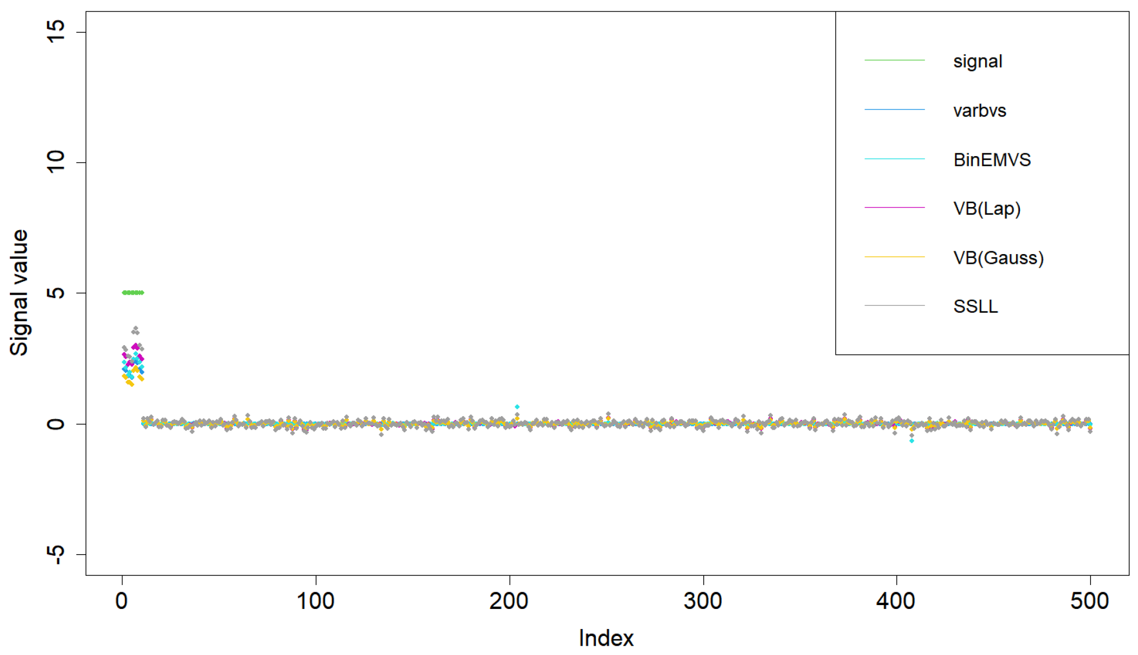
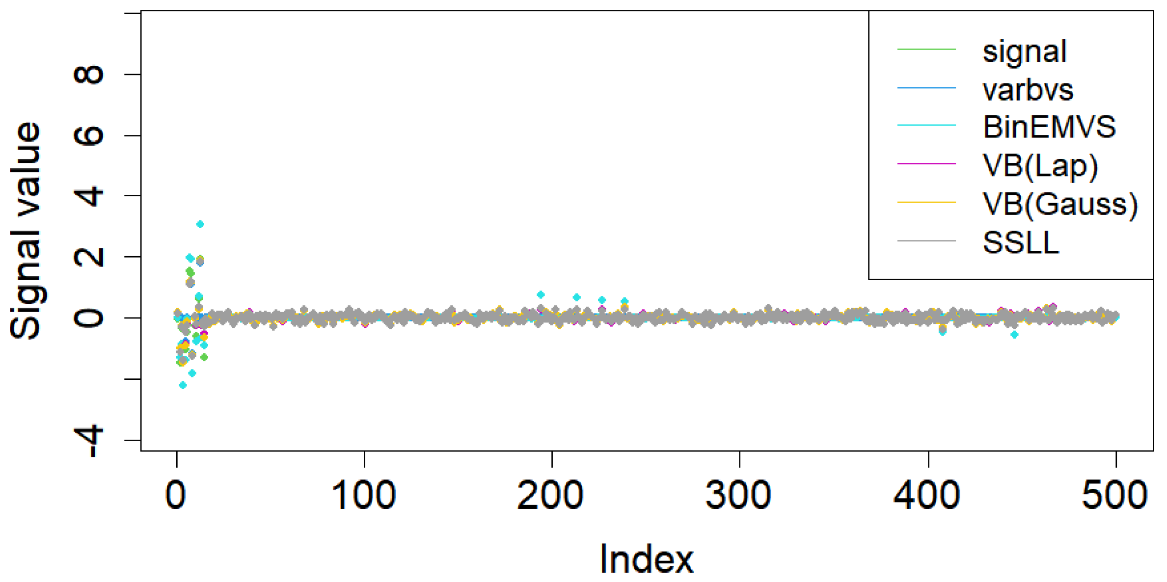
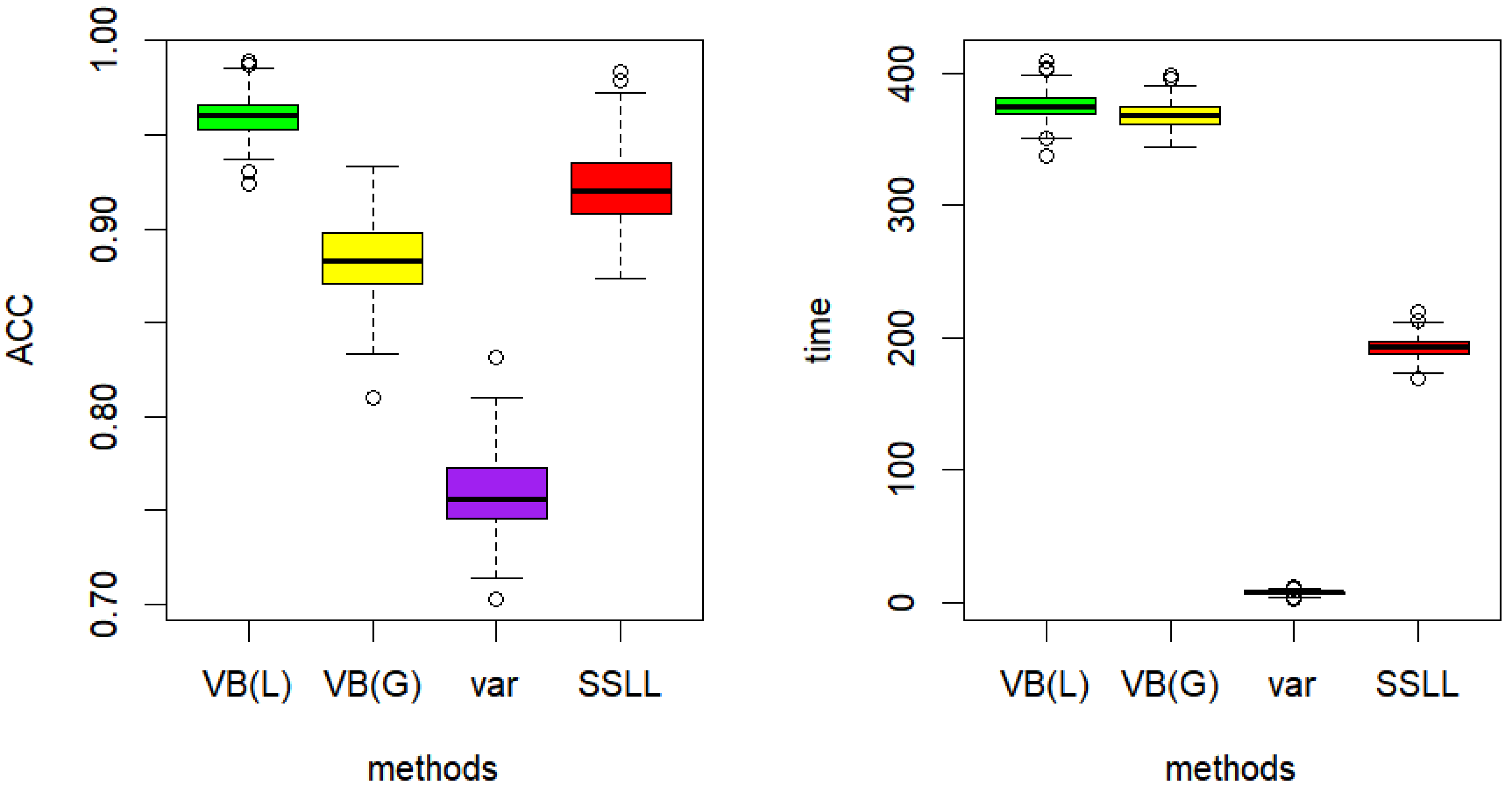
5.1. Simulation Study

We consider three data generation models, where $X_{ij}$$(j=2,\dots ,p+1)$ are independently drawn from a standard normal distribution, and $X_{i1}=1$ for $i=1,2,\dots ,n$. The simulated data are generated by the logistic model: $logit\left(u_i\right)=log\left(u_i/(1-u_i)\right)={\mathbf{X}}_i^{\mathrm{T}}\mathit{\beta }$, and $y_i$ is sampled from a Bernoulli distribution $Bernoulli\left(u_i\right)$. The values and sparsity levels of $({\beta }_0=1,{\beta }_1,\dots ,{\beta }_s,{{\displaystyle \underbrace{0,\dots ,0}}}_{p-s})$ are as follows: (1) ${\beta }_1=\dots ={\beta }_s=5$, $s=10$, $n=300$, $p=500$; (2) ${\beta }_1,\dots ,{\beta }_s$ are i.i.d. from the uniform distribution $U(-2,2)$, $s=15$, $n=300$, $p=500$; (3) ${\beta }_1=\dots ={\beta }_s=10$, $s=25$, $n=3000$, $p=5000$.

We compare the following methods: specifying that both ${\phi }_1\left({\beta }_j\right)$ and ${\phi }_0\left({\beta }_j\right)$ follow normal distributions in the spike-and-slab prior, using BinEMVS [26] (R package BinaryEMVS) for variable selection based on the EM algorithm; using the same prior but with varbvs [14] (R package varbvs) for variable selection via variational Bayesian inference; specifying ${\phi }_1\left({\beta }_j\right)$ as normal in the spike-and-slab prior, using VB (Gauss) [22] (R package sparsevb) for variational Bayesian variable selection; and specifying ${\phi }_1\left({\beta }_j\right)$ as Laplace in the spike-and-slab prior, using VB (Lap) [22] (R package sparsevb). We also compare with Bayesian Lasso (BL) for logistic regression (R package BayesLogit).

The hyperparameter settings follow those in the original references. The method proposed in this paper (SSLL) uses priors with $a_0=1,b_0=1,c_1=1,d_1=1,c_0=100,$ $d_0=1$. In our variational Bayes framework, when p is large, explicitly enumerating and reporting all $2^p$ model probabilities becomes computationally infeasible and difficult to interpret. For example, when $p=20$, the total number of possible models exceeds one million. Therefore, instead of listing all model probabilities, we summarize the posterior marginal inclusion probabilities $\mathbb{E}\left[{\gamma }_j\right]$ for each covariate, which is a widely accepted and interpretable measure in high-dimensional Bayesian variable selection. Moreover, as our method is based on variational inference rather than MCMC, we approximate the posterior distribution using a fully factorized mean-field family. Therefore, joint posterior model probabilities are not directly available as in an MCMC-based model averaging, but the marginal inclusion probabilities ${\varphi }_j=\mathbb{E}\left[{\gamma }_j\right]$ still provide informative summaries of variable relevance.

We define ${\varphi }_j={\mathbb{E}}_q\left[{\gamma }_j\right]$ as the approximate posterior inclusion probability for variable j, where ${\gamma }_j\in \{0,1\}$ indicates the selection status. These are marginal probabilities and do not correspond to the posterior probability of a particular model. Following standard practice, we apply a threshold ${\varphi }_j>0.5$ as a heuristic criterion for variable inclusion; while this is a convenient and interpretable rule, we emphasize that it does not reflect the selection of a single most probable model, but rather identifies variables with high marginal support across the model space. Hence, any weak Beta prior with initial expectation $\mathbb{E}\left[\pi \right]=a_0/(a_0+b_0)=0.5$ is acceptable. In high-dimensional settings, choosing $a_0=1$ and $b_0=p$ is known to yield an optimal posterior [11]. The parameters $c_1,d_1,c_0,d_0$ are selected such that the expectations satisfy ${\lambda }_1$ (smaller value) and ${\lambda }_0$ (larger value), respectively.

We primarily focus on variable selection and prediction. The evaluation metrics include True Positives (TPs), estimation error $\parallel \beta -\widehat{\beta }{\parallel }_2$ ($L_2$ norm), mean squared prediction error

$${\left({\displaystyle \frac{1}{n}}\sum _{i=1}^n{\left(\sigma \left({\mathit{X}}_i^{\mathrm{T}}\mathit{\beta }\right)-\sigma \left({\mathit{X}}_i^{\mathrm{T}}\widehat{\mathit{\beta }}\right)\right)}^2\right)}^{1/2}\left(\mathrm{PMSE}\right),$$

and runtime T (in seconds). The results are averaged over 20 runs, with standard errors in parentheses.

Table 1. Comparison of sparse Bayesian methods in high-dimensional logistic regression (${\beta }_1=\dots ={\beta }_s=5,s=10,n=300,p=500$. Results averaged over 500 replicates).

Methods	TP	${\mathit{L}}_2$	MSPE	T
BinEMVS	$1.00$	9.134	0.095	33.807
	(0.00)	(0.011)	(0.001)	(10.196)
VB (Lap)	$1.00$	8.218	0.145	3.683
	(0.00)	(0.050)	(0.001)	(0.033)
VB (Gauss)	$1.00$	10.841	0.150	3.087
	(0.00)	(0.010)	(0.001)	(0.034)
varbvs	$1.00$	9.532	0.086	2.118
	(0.00)	(0.000)	(0.000)	(0.053)
SSLL	$1.00$	7.012	0.113	1.165
	(0.00)	(0.031)	(0.020)	(0.018)
BL	$1.00$	9.012	0.121	30.552
	(0.00)	(0.052)	(0.031)	(1.325)

presents results for the first data generation model. All methods achieve perfect TP (1.00) across 500 simulations, indicating no important variables were missed. Regarding parameter estimation, SSLL attains the smallest $L_2$ error. Figure 1 shows the true coefficients ${\beta }_1=\dots ={\beta }_s=5$ (signal, green), where SSLL produces superior estimates, reflecting its adaptability as an SSL prior. However, all methods tend to underestimate $\beta$, likely due to the independence assumption among parameters. Prediction performance is comparable across methods. Runtime-wise, BinEMVS (EM-based) is the slowest. SSLL expresses the Laplace prior as a mixture of normal and exponential distributions, which improves estimation accuracy and computational speed. Although Bayesian Lasso remains a popular baseline, it can be computationally expensive in high-dimensional logistic regression, motivating our use of scalable shrinkage priors and variational inference for efficiency without sacrificing predictive performance.

Table 2. Comparison of sparse Bayesian methods in high-dimensional logistic regression (${\beta }_1,\dots ,{\beta }_s\sim U(-2,2),s=15,n=300,p=500$. Results averaged over 500 replicates).

Methods	TP	${\mathit{L}}_2$	MSPE	T
BinEMVS	0.80	3.231	0.258	40.028
	(0.00)	(0.178)	(0.003)	(0.945)
VB (Lap)	0.67	2.756	0.126	3.234
	(0.00)	(0.040)	(0.001)	(0.096)
VB (Gauss)	0.68	2.812	0.134	3.217
	(0.02)	(0.012)	(0.001)	(0.053)
varbvs	0.60	1.984	0.215	3.328
	(0.00)	(0.000)	(0.000)	(0.124)
SSLL	0.70	2.150	0.133	2.231
	(0.00)	(0.001)	(0.001)	(0.037)
BL	0.60	2.321	0.233	41.621
	(0.00)	(0.002)	(0.005)	(1.054)

reports results for the second data generation model, where nonzero ${\beta }_j$ are drawn from $U(-2,2)$. This model poses a greater challenge for variable selection. According to the TP results, methods select most but not all important variables. This is because variable selection probabilities ${\varphi }_j$ depend on the magnitude of ${\beta }_j$; smaller true values lead to lower selection probabilities and, thus, exclusion.

From Table 2, it can be seen that BinEMVS attains the highest TP (0.80), followed by SSLL (0.70), outperforming VB and varbvs methods. Varbvs achieves the lowest $L_2$ error (1.984), with SSLL close behind (2.150), indicating competitive parameter estimation. SSLL also records a low MSPE (0.133), better than BinEMVS and BL, and comparable to VB methods. Notably, SSLL has the shortest runtime (2.231 s), which is substantially faster than BinEMVS and BL (both over 40 s) and more efficient than VB and varbvs. Overall, SSLL balances variable selection accuracy, estimation precision, and predictive performance with superior computational efficiency, highlighting its practical advantage for sparse modeling in high-dimensional logistic regression.

Figure 2 shows estimated coefficients compared to the true signals (green). The SSLL method performs comparably to others, with generally smaller estimation errors than in the first model, possibly due to randomness in nonzero coefficients. The SSLL method also exhibits strong prediction and high computational efficiency.

Table 3. Comparison of sparse Bayesian methods in high-dimensional logistic regression (${\beta }_1=\dots ={\beta }_s=10,s=25,n=3000,p=5000$. Results averaged over 500 replicates).

Methods	TP	${\mathit{L}}_2$	MSPE	T
BinEMVS	∖	∖	∖	∖
	∖	∖	∖	∖
VB (Lap)	1.00	10.623	0.031	383.532
	(0.00)	(0.050)	(0.001)	(10.033)
VB (Gauss)	1.00	15.247	0.136	367.145
	(0.00)	(0.010)	(0.002)	(9.623)
varbvs	1.00	29.126	0.212	7.856
	(0.00)	(0.000)	(0.000)	(0.522)
SSLL	1.00	14.217	0.075	175.144
	(0.00)	(0.031)	(0.030)	(0.312)
BL	∖	∖	∖	∖
	∖	∖	∖	∖

summarizes the results for the third data generation model with $p=5000$. Due to computational cost, the BinEMVS and BL methods are excluded. VB (Lap) shows strong variable selection, parameter estimation, and prediction performance, but is relatively slow because it estimates each ${\beta }_j$ element-wise, which scales poorly with p; while varbvs is fast, it suffers from higher estimation and prediction errors. The SSLL method serves as a practical compromise between accuracy and computational efficiency.

5.2. Actual Data Analysis

We analyze a breast cancer dataset detailed by Van et al. [27], also available in the R package breastCancerNKI. The dataset comprises 295 women with breast cancer and 4919 gene microarray mRNA expression measurements (selected from 24,885 reliably expressed genes). Among these patients, 88 experienced cancer metastasis after systemic adjuvant therapy. We use the 4919 gene expressions as predictors in a logistic regression model to predict metastasis. All explanatory variables were standardized prior to model fitting.

Although variable selection is an integral part of the modeling process, we do not emphasize the specific genes selected, for two reasons. First, the high dimensionality (4919 genes vs. 295 samples) makes the selection sensitive to sampling variability and prior choices, and variable selection is known to be unstable in such settings with no unique “correct” predictor set. Second, the primary goal is accurate metastasis prediction rather than biological interpretation. Thus, we focus on evaluating predictive performance using cross-validation metrics including area under the ROC curve (AUC) and classification accuracy.

Nevertheless, we use a sparsity-inducing prior (e.g., spike-and-slab Laplace) to regularize the model and encourage parsimony. Though selected genes vary across subsamples, the predictive performance remains robust, suggesting stable predictive patterns captured by the model. For the logistic regression model, prediction accuracy is measured as

$$ACC={\displaystyle \frac{1}{n}}\sum _{i=1}^n\left|y_i-\sigma \left({\mathbf{X}}_i^{\mathrm{T}}\beta \right)\right|,i=1,2,\dots ,295,$$

where “positive” cases ($y_i=1$) indicate metastasis after treatment, and “negative” cases ($y_i=0$) indicate no metastasis.

Due to computational constraints, BinEMVS and BL are excluded from this analysis. Figure 3 compares prediction accuracy and runtime for VB (Lap), VB (Gauss), varbvs, and SSLL, mirroring the simulation results with $p=5000$. The runtime of SSLL here is shorter than in the simulation (where $n=3000$ vs. $n=295$ here), benefiting from the use of the Woodbury formula to reduce the computational cost of large matrix operations, thereby speeding up execution.

To evaluate out-of-sample prediction, we performed 5-fold stratified cross-validation, preserving the proportion of positive cases (metastasis) within each fold. Each iteration trains on four folds and tests on the remaining one. Predictive performance is measured by PMSE and AUC, with means and standard deviations reported across folds.

Figure 4 shows that SSLL achieves the highest mean AUC, indicating superior discrimination between positive and negative cases. VB (Lap) performs similarly, with AUC only slightly lower than SSLL. VB (Gauss) and varbvs lag behind by a modest but wider margin. These results confirm that SSLL provides the strongest predictive performance under repeated data splits, establishing a benchmark for the competing methods.

6. Conclusions

In Bayesian variable selection, we apply the SSL prior to high-dimensional logistic regression models. Utilizing a fast variational Bayes (VB) algorithm, we perform posterior inference on model parameters. Notably, both the lower bound approximation approach and the introduction of Pólya-Gamma variables lead to the same VB update scheme. Based on simulation studies and real data analysis, the variational Bayesian variable selection algorithm under the SSL prior exhibits several key advantages: (1) the adaptive shrinkage of coefficients, with weak shrinkage for important covariates and strong shrinkage for unimportant ones; (2) simultaneous parameter estimation and variable selection with low computational cost, where the posterior variance (or covariance) of parameters is naturally obtained; (3) no need for manual parameter tuning, as both the penalty parameter $\lambda$ and the model parameters $\beta$ are estimated jointly; (4) the use of the Woodbury matrix identity, which circumvents large matrix operations.

The SSL prior combines the strengths of the Lasso and spike-and-slab priors, while mitigating their individual limitations. As such, it provides a flexible and powerful framework that can be extended to more complex models. In this work, and in related methods, we assume parameter independence for simplicity and tractability. Although relaxing this assumption might improve estimation accuracy, it would also introduce significant complexity in modeling and computation. Thus, this simplification represents a practical trade-off.

The SSL prior framework holds substantial potential for extension to more sophisticated modeling scenarios. As a hybrid approach incorporating both continuous and discrete shrinkage components, it can be naturally generalized to a variety of advanced statistical models. Potential directions include hierarchical models with structured random effects, where SSL priors may facilitate multi-level variable selection, and semi-parametric additive models, where they could enable joint selection of both linear and nonlinear components. Additionally, extensions to multivariate response models, such as multinomial logistic regression for categorical outcomes or zero-inflated models for count data, are promising. Thanks to the computational efficiency of the variational Bayes implementation, the method can scale effectively to these more complex settings. These extensions underscore the versatility of the SSL prior while retaining its core strengths: automatic parameter tuning, adaptive shrinkage, and computationally efficient posterior approximation.

References

1. Bishop, C.M. Pattern Recognition and Machine Learning; Springer: New York, NY, USA, 2006. [Google Scholar]
2. Tibshirani, R. Regression shrinkage and selection via the lasso. J. R. Stat. Soc. Ser. (Methodol.) 1996, 58, 267–288. [Google Scholar] [CrossRef]
3. Fan, J.; Li, R. Variable selection via nonconcave penalized likelihood and its oracle properties. J. Am. Stat. Assoc. 2001, 96, 1348–1360. [Google Scholar] [CrossRef]
4. Zhang, C.H. Nearly unbiased variable selection under minimax concave penalty. Ann. Stat. 2010, 38, 894–942. [Google Scholar] [CrossRef]
5. Casella, G.; Ghosh, M.; Gill, J.; Kyung, M. Penalized regression, standard errors, and Bayesian lassos. Bayesian Anal. 2010, 5, 369–411. [Google Scholar] [CrossRef]
6. Hans, C. Bayesian lasso regression. Biometrika 2009, 96, 835–845. [Google Scholar] [CrossRef]
7. Li, Q.; Lin, N. The Bayesian elastic net. Bayesian Anal. 2010, 5, 151–170. [Google Scholar] [CrossRef]
8. George, E.I.; McCulloch, R.E. Variable selection via Gibbs sampling. J. Am. Stat. Assoc. 1993, 88, 881–889. [Google Scholar] [CrossRef]
9. Roková, V. Bayesian estimation of sparse signals with a continuous spike-and-slab prior. Ann. Stat. 2018, 46, 401–444. [Google Scholar] [CrossRef]
10. Mitchell, T.J.; Beauchamp, J.J. Bayesian variable selection in linear regression. J. Am. Stat. Assoc. 1988, 83, 1023–1032. [Google Scholar] [CrossRef]
11. Castillo, I.; van der Vaart, A. Needles and straw in a haystack: Posterior concentration for possibly sparse sequences. Ann. Stat. 2012, 40, 2069–2101. [Google Scholar] [CrossRef]
12. Roková, V.; George, E.I. The spike-and-slab lasso. J. Am. Stat. Assoc. 2018, 113, 431–444. [Google Scholar] [CrossRef]
13. Bai, R.; Rockova, V.; George, E.I. Spike-and-slab meets lasso: A review of the spike-and-slab lasso. arXiv 2020, arXiv:2010.06451. [Google Scholar]
14. Carbonetto, P.; Stephens, M. Scalable variational inference for bayesian variable selection in regression, and its accuracy in genetic association studies. Bayesian Anal. 2012, 7, 73–108. [Google Scholar] [CrossRef]
15. Huang, X.; Wang, J.; Liang, F. A variational algorithm for Bayesian variable selection. arXiv 2016, arXiv:1602.07640. [Google Scholar]
16. Ray, K.; Szabó, B. Variational Bayes for high-dimensional linear regression with sparse priors. J. Am. Stat. Assoc. 2022, 117, 1270–1281. [Google Scholar] [CrossRef]
17. MacKay, D.J.C. The evidence framework applied to classification networks. Neural Comput. 1992, 4, 720–736. [Google Scholar] [CrossRef]
18. Jaakkola, T.S.; Jordan, M.I. Bayesian parameter estimation via variational methods. Stat. Comput. 2000, 10, 25–37. [Google Scholar] [CrossRef]
19. Wang, C.; Blei, D.M. Variational inference in nonconjugate models. J. Mach. Learn. Res. 2013, 14, 1005–1031. [Google Scholar]
20. Polson, N.G.; Scott, J.G.; Windle, J. Bayesian inference for logistic models using Pólya–Gamma latent variables. J. Am. Stat. Assoc. 2013, 108, 1339–1349. [Google Scholar] [CrossRef]
21. Zhang, C.X.; Xu, S.; Zhang, J.S. A novel variational Bayesian method for variable selection in logistic regression models. Comput. Stat. Data Anal. 2019, 133, 1–19. [Google Scholar] [CrossRef]
22. Ray, K.; Szabó, B.; Clara, G. Spike and slab variational Bayes for high dimensional logistic regression. Adv. Neural Inf. Process. Syst. 2020, 33, 14423–14434. [Google Scholar]
23. Tang, Z.; Shen, Y.; Zhang, X.; Yi, N. The spike-and-slab lasso generalized linear models for prediction and associated genes detection. Genetics 2017, 205, 77–88. [Google Scholar] [CrossRef] [PubMed]
24. Blei, D.M.; Kucukelbir, A.; McAuliffe, J.D. Variational inference: A review for statisticians. J. Am. Stat. Assoc. 2017, 112, 859–877. [Google Scholar] [CrossRef]
25. Wei, R.; Ghosal, S. Contraction Properties of Shrinkage Priors in Logistic Regression. J. Stat. Plan. Inference 2020, 207, 215–229. [Google Scholar] [CrossRef]
26. Mcdermott, P.; Snyder, J.; Willison, R. Methods for Bayesian Variable Selection with Binary Response Data using the EM Algorithm. arXiv 2016, arXiv:1605.05429. [Google Scholar]
27. Van De Vijver, M.J.; He, Y.D.; Va not Veer, L.J.; Dai, H.; Hart, A.A.; Voskuil, D.W.; Schreiber, G.J.; Peterse, J.L.; Roberts, C.; Marton, M.J.; et al. A Gene-Expression Signature as a Predictor of Survival in Breast Cancer. N. Engl. J. Med. 2002, 347, 1999–2009. [Google Scholar] [CrossRef]
Figure 1. Estimation of β in sparse Bayesian methods for high-dimensional logistic regression ( β 1 = = β s = 5 , s = 10 , n = 300 , p = 500 ).
Mathematics 13 02205 g001
Figure 2. Estimation of β in sparse Bayesian methods for high-dimensional logistic regression ( β 1 , , β s U ( 2 , 2 ) , s = 15 , n = 300 , p = 500 ).
Mathematics 13 02205 g002
Figure 3. Comparison of prediction accuracy and runtime for four methods on breast cancer data.
Mathematics 13 02205 g003
Figure 4. ROC curve comparison of four methods on breast cancer data.
Mathematics 13 02205 g004