Mathematical Modeling of Signals for Weight Control of Vehicles Using Seismic Sensors

Abstract

The article presents a new method of passive dynamic weighing of vehicles based on the registration of seismic signals that occur when wheels pass through strips specially applied to the road surface. Signal processing is carried out using spectral methods, including fast Fourier transform, consistent filtering, and regularization methods for solving inverse problems. Special attention is paid to the use of linear-frequency-modulated signals, which make it possible to distinguish the responses of individual axes even when superimposed. Field tests were carried out on a real section of the road, during which signals from vehicles of various classes were recorded using eight geophones. The average error in determining the speed of 1.2 km/h and the weight of 8.7% was experimentally achieved, while the correct determination of the number of axles was 96.5%. The results confirm the high accuracy and sustainability of the proposed approach with minimal implementation costs. It is shown that this system can be scaled up for use in intelligent transport systems and applied in real traffic conditions without the need to intervene in the design of the roadway.

1. Introduction

The development of transport infrastructure and the increase in the number of vehicles on the roads in recent decades have led to the aggravation of one of the most important technical and socio-economic problems—premature wear and destruction of the road surface [1,2]. Globally, a significant proportion of asphalt damage is caused by vehicle overloads that exceed permissible axle loads. This not only accelerates the depreciation of roads and increases the cost of their maintenance, but also reduces road safety, creates economic losses, and worsens the environmental situation [3]. In this regard, the task of accurate and operational control of vehicle parameters in the flow, such as weight, number of axles, and speed, is of fundamental importance for modern intelligent transport systems, especially in the context of increasing automation and digitalization of road infrastructure [4,5].

One of the widely used approaches to solving this problem is the use of weigh-in-motion (WIM) systems based on strain gauge, piezoelectric and fiber-optic sensors built into the road surface. Works [6,7,8,9], as well as [10], are examples of the successful implementation and assessment of the accuracy of such systems. In these works, empirically calibrated regression models are used, as well as Kalman filters, to eliminate dynamic fluctuations in the axial load. At speeds of up to 60 km/h, axle load measurement accuracy is up to ±7% and under favorable conditions up to 5% (COST 323 class A (5)). However, when the speed increases to 100 km/h, the accuracy decreases sharply (to ±10–12%), especially in conditions of uneven road surfaces, temperature differences, and lack of regular calibration. The high cost of installation, the need to intervene in the road structure, and the complexity of maintenance are also significant limitations of this approach. Mathematically, such systems require numerical solutions to the problems of time series processing, temperature drift compensation, and optimization of the weight coefficients of the calibration model [11].

Another area is systems that use radar and video analytical methods. For example, the paper edited by [12] describes radar technologies based on the processing of reflected signals and the application of Doppler shift equations [13]. These methods measure speed with an accuracy of ±2 km/h and classify vehicles by size with an accuracy of 90%. The mathematical apparatus of these systems includes spectral analysis methods, pattern matching algorithms, and machine learning for classification. However, the effectiveness of such systems decreases in conditions of fog, rain, and other weather factors, as well as when obscuring objects [14].

In recent years, there has been a growing interest in passive recording methods, in particular, seismic recording of signals from vehicles. Such approaches have a number of advantages: they do not require radiation, they do not depend on visibility and weather conditions, and their implementation can be relatively inexpensive. A number of studies [15,16,17,18,19,20] show that the use of seismic sensors makes it possible to determine the speed of movement with an accuracy of ±1.5–2 km/h and to classify vehicles by the number of axles and weight with an accuracy of 85–95% in the speed range up to 80 km/h, corresponding to the impact of the wheels on the roadway. However, high sensitivity to external vibrations and difficulties in synchronizing signals from different sensors require the development of algorithms for space–time filtering and time alignment [21].

To improve the efficiency of seismic methods, an approach to spectral analysis of signals recorded by geophones was proposed, which made it possible to significantly improve the accuracy of identification. Works [22,23,24,25,26] demonstrate the possibility of distinguishing vehicle types with an accuracy of up to 90–95%, while noise immunity is achieved through the use of filtering, statistical processing, and machine learning methods. In these studies, models based on wavelet analysis, principal component analysis (PCA) methods, power spectral density estimation, as well as vector support algorithms (SVMs) and decision trees are used. Processing includes the construction of vector features based on energy content in certain frequency ranges, which makes it possible to use classification methods on a set of training data [27]. Such approaches are especially useful in the presence of a background and intersecting signals, as they allow you to effectively isolate the informative components of the signal.

A separate category is made up of methods that use neural network architectures. Studies [15,28,29,30,31,32] demonstrate the effectiveness of convolutional neural networks (CNNs), recurrent neural networks (RNNs), and hybrid structures for classifying vehicles by their seismic signatures. The achieved classification accuracy in these works is up to 95% at speeds up to 80 km/h, while the resistance to external noise remains at the level of 80–85%. Using these models requires deep training on a large volume of stamps and pre-normalizing the data. Neural network training is accompanied by the use of loss functions, such as cross-entropy, and optimization using gradient descent algorithms (Adam, RMSprop), which requires significant computational resources [33].

Some studies are aimed at reconstructing the trajectories of movement and determining the mass of vehicles without the use of embedded sensors. In the works [16,34,35], methods of temporal correlation of signals from several sensors are used; the problems of inverse modeling of the trajectory and the use of Kalman filters are solved. Mass estimation is carried out on the basis of the amplitude component of the seismic signal and numerical solution of the reversal problem, while an accuracy of less than 10% is achieved at speeds up to 60 km/h.

A comparative analysis of all the above approaches allows us to identify a common problem: either the high cost and complexity of implementation, as in WIM systems, or the limited accuracy in noise and multi-signal conditions, as in passive methods. In the mathematical aspect, these problems are reduced to multivariate models of signal processing, namely, to the problems of regression, optimization, identification, and inverse problems. The relevance of further research in this direction is due to the need to develop solutions that would provide accurate determination of vehicle parameters without expensive engineering solutions [36,37] and with the possibility of scalable implementation.

Of particular interest is passive seismic recording of signals from the interaction of vehicles with artificially created irregularities (stripes) on the roadway. This approach allows both the generation of a signal with pronounced spectral characteristics and the simplification of subsequent processing. Strips of a certain width and shape apply to the coating to induce resonant or impulse signals when the wheel hits it, which greatly simplifies the task of synchronization and interpretation. The use of such structures simulating combs with a uniform or non-uniform pitch is described in theoretical and experimental studies, which confirm the possibility of increasing the accuracy of measuring the speed and number of axes up to 95% and estimating the mass with an error of less than 10% at a speed of up to 70 km/h, as well as frequency analysis of responses.

Thus, the direction proposed in this work, based on the passive registration of seismic signals caused by the passage of a vehicle through artificial strips, has a high degree of feasibility and accuracy. Its main advantage is that there is no need to costly integrate sensors into the road structure while maintaining high measurement accuracy and resistance to interference. The mathematical novelty of the proposed approach lies in the fact that a model of the seismic signal is formed as a superimposition of responses from periodically located sources, which makes it possible to use devices for coordinated filtering, analysis of flight time, and localization along the maximum spectrum. In this work, it is planned to build an analytical and numerical model for generating a seismic signal from the movement of a vehicle on a striped structure, using the Fourier transform and algorithms for extracting phase characteristics, as well as estimating the parameters of the vehicle by solving the inverse problem based on minimizing the error functional between the model and the recorded signal.

The purpose of this work is to develop a mathematical model of a system for dynamic determination of vehicle parameters based on the passive seismic location. Within the framework of this goal, seismic signals arising from the interaction of vehicles with artificially created structures on the roadway are simulated, and the possibilities for determining the speed, number of axles, axle load, and total weight of the vehicle are analyzed. It is proposed to use the integration of spectral analysis methods, consistent filtering, regularized optimization, and verification of the model on experimental data to improve the accuracy and stability of results in real operation.

2. Materials and Methods

Within the framework of this study, a system for dynamic determination of vehicle parameters based on passive seismic location was developed and experimentally tested, implemented both on the basis of physical modeling and with the use of an extensive mathematical apparatus for signal analysis, parameter estimation, and inverse problem solving. The purpose of this work is not only to record the seismic response from the movement of the vehicle but also to restore such parameters as speed, number of axles, axle load, and total weight using formalized mathematical models. The experimental part of the study is based on the combination of field measurements with subsequent computer signal processing using MATLAB (version 2023b) and the authors’ program code that implements filtering, Fourier transform, and consistent filtering methods.

To record seismic signals, vertical geophones were used, integrated into the roadway in areas with special artificial stripes. The type of geophones used corresponds to the industrial sensitivity class (up to 70–80 dB of the dynamic range), and their amplitude–frequency response provided stable registration of oscillations in the range from 5 to 150 Hz. The signal from the sensors was transmitted to the pre-processing system, which included an amplifier and an analog-to-digital converter (16-bit, 520 Hz), and transmitted to the central computing module via an IP connection. The arrangement of the stripes, which is a comb structure with a uniform or uneven pitch, as well as the placement of geophones, made it possible to record the signals arising when the wheels of the vehicle hit the strips, ensuring the formation of high-amplitude seismic waves.

The experiments involved simulating the movement of a vehicle with specified parameters (number of axles, distance between wheels, speed, weight) and registering the corresponding signals. In some cases, vehicles with pre-known parameters were used, which made it possible to calibrate the mathematical model. The processing system used included signal whitening, spectral analysis, and time boundary estimation of pulsed fragments using a sliding window instantaneous power estimate. To improve the accuracy of the analysis, timestamp synchronization algorithms and a method for estimating speed using time delays between signal edges on different sensors were used.

The basis of the mathematical model is the representation of the seismic response as a superimposition of responses from each “wheel–strip” pair. The signal on each of the sensors is modeled according to the formula:

$$s_i(t)={\displaystyle \sum _{j=1}^J{\displaystyle \sum _{n=1}^N{h}_{ijn}}}{f}_{ijn}(t-{\tau }_{ijn}),$$

where $h_{ijn}$ is the amplitude multiplier determined by the distance from the strip to the sensor, $f_{ijn}\left(t\right)$ is the impulse response, ${\tau }_{ijn}$ is the propagation delay, J is the number of bands, and N is the number of axes. The response $f_{ijn}\left(t\right)$ is described as a damped function:

$$f_{ijn}(t)=A_{ijn}{e}^{-\alpha t}\sin (\omega t),$$

where the damping factor α and angular frequency ω are determined by the effective mechanical properties of the layered structure comprising the asphalt pavement, its base layers, and the underlying soil. While the seismic wave propagates through the pavement structure, experimental and numerical studies (e.g., [38]) show that the dominant influence on attenuation and resonance frequency stems from the stiffness and damping characteristics of the asphalt layer, including bitumen content, aggregate size, and thickness. Thus, α and ω are treated as effective parameters that are calibrated using signals from reference vehicles and take into account both the pavement and soil structure.

The simulation was carried out both using analytical formulas and using the MATLAB code provided in Appendix A. Time delays ${\tau }_{ijn}$ were calculated according to geometric relationships, taking into account the coordinates of the bands and sensors:

$${\tau }_{ijn}={\displaystyle \frac{\sqrt{{(x_j-x_i)}^2+{(y_j-y_i)}^2}}{v_g}},$$

where v_g is the speed of propagation of the seismic wave.

To identify the parameters of the vehicle, the inverse problem of minimizing the deviation between the measured signal $s_i^{\mathrm{meas}}(t)$ and the model response was formulated:

$$\underset{M,v,d_n}{\min }{\displaystyle \sum _i\left|\right|s_i^{\mathrm{meas}}(t)-s_i(t;M,v,d_n)|{|}_2^2}.$$

The solution of this problem was carried out by numerical optimization methods using Tikhonov’s regularization:

$$\min (||A\theta -b|{|}_2^2+\lambda \left|\right|\theta |{|}_2^2),$$

where A is the feature matrix, θ is the parameter vector, b is the measured power values, and λ is the regularization parameter.

Two approaches were used to estimate the velocity. The first is spectral, in which the distance between the harmonics of the spectrum Δϕ determines the velocity:

$$v=\Delta x{\displaystyle \frac{f_s}{k_2-k_1}},$$

where Δξ is the spacing between the bands; f_s is the sample rate; and k₂, k₁ are the harmonic numbers. The second is temporary, using the delay between the edges of the signals from the two bands:

$$v={\displaystyle \frac{L}{\Delta t}},$$

where L is the distance between the strips, and Δτ is the delay. Synchronization to the maximum of the coordinated filtering was also used to localize the impact time of each axis.

In addition, the mass estimation error was estimated, which depended on the accuracy of the seismic signal power measurement. The model used assumed the presence of noise ϵ~$\mathcal{N}$(0, σ2), and the mass was estimated as:

$$\widehat{M}=\sqrt{{\displaystyle \frac{P-ϵ}{\beta }}},$$

which implied the calibration of the parameter against reference vehicles.

As a test, a system installed on the Sovetskoye Highway was used, with eight geophones and two types of markings. Real signals from seven trucks were processed. Based on the analysis of their spectral, temporal, and amplitude characteristics, estimates of the speeds, mass, and number of axes were obtained. The error in determining the speed did not exceed 1.2 km/h, and the error in weight was 8.7% at speeds up to 70 km/h. The accuracy of the classification of the number of axles reached 96.5%. Thus, the developed system combines physical modeling, experimental verification, and rigorous mathematical processing, including spectral analysis, optimization methods, signal processing, and inverse problem solving.

The values of damping and frequency parameters used in signal modeling were determined empirically during field calibration on asphalt pavement, using reference vehicles with known weight and speed. This approach accounts for the layered structure of the road, including asphalt and its subbase, and incorporates their combined impact on seismic wave attenuation and frequency response.

3. General Information About Passive Seismic Location

The theory of passive seismic location is now at the initial stage of its development. Despite the many significant differences between radar and passive seismic location, there is a basic relationship between them, determined by the commonality of the tasks to be solved. The random nature of interference and useful signals is due to the use of statistical approaches in the theory of passive seismic location, as well as in radar, which have been duly applied and developed in the PSL.

For a long time, seismic technology has been successfully used to explore Earth in search of minerals. As a rule, these technologies are active, and their operation requires the use of powerful sources of seismic signals. Seismic vibrations are received by a group of seismic sensors, and the general analysis of the received signals allows you to analyze the structure of the medium in which seismic waves propagate.

At the moment, seismic signals are quite widely used for detection when organizing the protection of territory. The sensors record and then process the signals that occur in the ground when someone crosses the protected area. Most of the known seismic protection systems are passive, since their principle of operation is not related to the emission of any signals. Compared to the geophysical application of seismic methods, the appearance of seismic waves in systems for monitoring moving objects is not associated with the use of devices that specifically create seismic fields. In this regard, seismic systems based on the detection of waves, the appearance of which is not associated with deliberate primary excitation but is due to the movement of objects, are passive.

Passive seismic location (PSL) is one of the new methods of radar observation. The processing of these signals is carried out on the basis of statistical methods, since they have a pronounced random nature.

When analyzing the received seismic signals, it is possible to solve problems that are aimed at obtaining information about moving objects. The main facts of the received seismic signals are the presence or absence of an object in the observation area, determining the type of moving object, calculating the coordinates and characteristics of its movement, as well as determining the weight characteristics. Determination of weight characteristics is a topic in which both owners and builders of highways have recently been interested. It is necessary to ensure the integrity and safety of roads, in accordance with numerous standards, as well as to achieve road safety.

It is clear that if an overloaded truck is driving on the road, which puts more pressure on the road than it is able to withstand, then the road begins to collapse. This project, based on passive seismic location to determine weight characteristics, is designed to identify such intentionally or unintentionally overloaded vehicles in order to stop them, stop their movement, and force drivers and (or) owners to move part of the cargo to another vehicle.

The task of this project is to create a mathematical model describing the movement of a vehicle based on measurements of the parameters of the seismic signal arising from the interaction of the wheels of the car with artificial obstacles (stripes) applied to the road surface, designed to establish the fact of the passage of the vehicle and assess some of its parameters, namely:

• the speed of the vehicle (at the time of measurement);
• the number of axles of the vehicle;
• the load on the axles of the vehicle;
• the total weight of the vehicle.

4. Physical Foundations of Passive Seismic Location

The physical basis of passive seismic location is the excitation of seismic waves in the surface layers of the soil by an object moving along it and their registration by receiving devices. The received signals have a pronounced random nature, and useful location information lies in the parameters of the signals. Therefore, an integral part of the location process is special processing of seismic signals, performed by computing devices structurally integrated into the equipment of the seismic radar system.

The calculation of the weight parameters of the vehicle, made with the technology of assessing the power of the seismic signal, is possible only in a dynamic mode, when the force of pressure on the ground changes, since only in this case is a seismic wave propagating in the ground formed, depending on the mass of the vehicle through some multiplier that affects only their amplitude, which is the main reason to assume that the power (amplitude) of the seismic signal is a sufficient statistic to measure the weight of the vehicle.

Let:

$$F(t)=Ma(t),$$

where M is the mass of the vehicle, and a(t) is the acceleration caused by hitting an obstacle. The signal generated at the point of impact can be described as a temporary convolution:

$$s(t)={\displaystyle \int h(\tau )}F(t-\tau )d\tau ,$$

where h(t) is the momentum characteristic of the medium, describing the reaction of the soil to a single impulse action. For numerical simulation, h(t) can be represented as an attenuated sine wave:

$$h(t)=A{e}^{-\alpha t}\sin (\omega t),$$

(1)

where A, α, ω are parameters that depend on the density and elasticity of the soil.

The structural diagram of the dynamic weighing system proposed by the authors is shown in Figure 1.

In Figure 1, k and c indicate the stiffness coefficient and reduce (prevent) oscillations of the weighing system, M is the weight of the car, m is the mass of the table, and x is forced oscillations in the system (displacement of the weighing system). It is this signal that propagates in the ground in the form of a seismic wave.

5. Functional Diagram of the Measuring Setup and Seismic Signal Processing Structure

The main problem is to measure the load parameter on the axles of the vehicle. The idea presented in this paper is to measure the dynamic effect F (t) exerted by the wheels of a vehicle on the road surface. This measurement is made on the basis of measuring the power of the seismic vibration caused by the interaction of the wheels of the car with the road surface using seismic sensors (vertical geophones).

The geophone is a speed sensor and is installed in the ground (in this case, the sensor is mounted in the pavement). The structure of the geophone is shown in Figure 2.

The signal from the vehicle recorded by the geophone (after appropriate digital processing) is the source of information about the axle load of the vehicle. The total weight of the vehicle is estimated based on the measured axle loads.

A variant of the installation proposed by the authors, which makes it possible to measure with sufficient accuracy the power of seismic oscillation associated with the dynamic impact of the axles of the car on the road surface, is shown in Figure 3.

The main purpose of the elements of the installation diagram (Figure 3) is as follows. With the help of a geophone (1), the signal is recorded in analog form, and these signals are transmitted via cables (2) to the pre-processing device (3), which performs amplification, filtering, and digitization of the signal with a clock speed of f₀ = 520 Hz and 16 bits/sample. The amplitude–frequency response of the geophone is shown in Figure 4. Element (4) represents the central computing module (PC or microcontroller system) that receives digital seismic signal data from the pre-processing unit and executes the algorithms for filtration, spectral analysis, and vehicle parameter estimation. Element (5) denotes a video camera system synchronized with the signal processing module, which captures images of the vehicle when the measured parameters (e.g., axle load or total weight) exceed predefined thresholds.

The geophones convert ground vibrations into analog voltage signals, which are transmitted via shielded signal cables to the pre-processing unit. Although analog signals are indeed sensitive to environmental noise and electromagnetic interference, this effect is minimized through the use of low-noise shielded twisted-pair cables and differential signal transmission. The pre-processing unit is located in close proximity (within 3–5 m) to the sensors to reduce signal degradation. Additionally, analog filtering and amplification are performed immediately before digitization to improve the signal-to-noise ratio. The decision to transmit the signal in voltage form prior to digitization was made to simplify the system architecture and maintain compatibility with industrial-grade geophones, which output voltage natively.

The choice of sample rate (and filter bandwidth) is determined by the spectrum band of the seismic signals that will be processed in the system. It is necessary to note the main dynamic range of seismic signals. Measurements show that with the use of amplification, the dynamic range of the recorded signals is at least 70–80 dB, so you need to use 16 bps/ch when digitizing them. The received readings via the IP interface are sent to the computer (4). A video camera (5) is used to fix the vehicle.

For adaptive processing of digital seismic signals, the following basic steps were proposed, performed in the form of an algorithm:

• Preliminary adaptive filtration (bleaching);
• Preliminary detection of the vehicle, including the assessment of its time limits in the signal (in refraction) as a result of nonlinear filtering of the initial signal (estimates of instantaneous power in a window of a given size) based on signals from geophones;
• Isolation of the impulse flux associated with the impact on an artificial obstacle (single lane) of the vehicle axes as a result of nonlinear filtering of the bleached signal (assessment of instantaneous power in a window of a given size) from geophones;
• Binding the boundaries of the vehicle signal to the pulses of the axes, estimating the number of axles of the vehicle;
• Assessment (by impulse flow) of the moment of time when the preliminarily detected vehicle reaches the section with multi-lane markings;
• Assessment of the load on the axles, the total weight of the vehicle, and its speed as a result of spectral processing of geophone signals located near multi-lane markings;
• Formation of data from the result of processing, checking the excess of the standard maximum weight of the vehicle and the load on its axles.

If the parameters specified in clause 7 exceed their maximum permissible values, the vehicle is fixed (a picture is taken); the image of the vehicle, as well as its parameters estimated on the basis of the seismic signal, is sent via the TCP/IP interface to the website of the Territorial Administration of Roads.

To estimate the weight M of the vehicle from the observed signal s(t), the average power shall be calculated:

$$P={\displaystyle \frac{1}{T}}{\displaystyle \underset{t_0}{\overset{t_0+T}{\int }}{s}^2(t)dt.}$$

Suppose that P~βΜ² + ϵ, where ϵ~$\mathcal{N}$(0, σ²) is the Gaussian noise, and β is the coupling coefficient. To estimate the mass M from noisy power measurements P, we consider the expectation E[P] = βΜ², since E[ϵ] = 0. In the presence of noise, the least squares estimate of M is computed from the sample mean of power observations as follows:

$$\widehat{M}=\sqrt{{\displaystyle \frac{\overline{P}}{\beta }}}$$

where

$$\overline{P}={\displaystyle \frac{1}{N}}{\displaystyle \sum _{i=1}^N{P}_i}$$

This estimation accounts for the random nature of noise ϵ, assuming multiple independent measurements P_i of signal power can be obtained. Then the weight estimate can be found by the least squares method:

$$\widehat{M}=\sqrt{{\displaystyle \frac{P-ϵ}{\beta }}}.$$

Since the power measurement is affected by additive noise, the mass estimation is based on averaging multiple observations to reduce the variance of the error. Assuming Gaussian noise, the best unbiased estimate of M is obtained using the mean of the observed power values. This approach aligns with the least squares method and improves the robustness of the estimation.

In Figure 5a, the possible layout of geophones and markings applied to the road surface is presented. Taking into account the structure of signal processing, its registration at the location of a single strip and multi-band marking is provided by three geophones.

6. Substantiation of the Marking Scheme Applied on the Carriageway

The goal of determining the parameters of the vehicle can be solved (within the framework of the proposed method) only in dynamics; static measurement of the weight of a stationary vehicle is impossible, since in this case, seismic vibrations do not occur in the ground, the power of which contains the basic information about the force of impact. In theory, the dynamic impact of Fd(t) can also be measured without the use of markings, for example, by measuring the average power of a seismic signal in a given time interval, since the passage of a car is a sequence of actions on the road surface through the contact patch of a wheel (Figure 5b). But still, this approach is fraught with many problems.

First, there is no way to separate the signals of the vehicle whose parameters we want to determine from the interference associated with passing vehicles, for example, on the oncoming lane or other seismic noise of the route interacting with the signal of interest.

Secondly, there are some problems of “binding” the vehicle to the corresponding signal. This problem is exacerbated by fairly dense traffic on multi-lane highways. Due to the overlapping of signals of vehicles at a close distance relative to each other, it is impossible to separate them. If the marking is applied on a certain strip, it makes it possible to create a seismic signal of a certain type, which differs in shape from the signals coming in the same time interval from other bands.

One possible way to improve the estimate is to create signals from the vehicle that are compact in the time or frequency domains. Such a signal can be a short pulse that can be realized as a result of creating an obstacle, for example, a narrow lane perpendicular to the direction of movement of the car.

It is clear that power measurement as a result of using such a signal in a narrow time interval will not lead to a critical hit of noise and interference in this interval. The stronger the impact on these bands, the greater the amplitude (power) of the desired signal and the higher the signal-to-noise ratio. However, this approach has its limitations related to the finite amplitude of the generated pulse. In addition, an increase in the amplitude of the impulse can be achieved by purely “physical” methods, for example, by increasing the height of the obstacle. However, an increase in the height of the obstacle is possible up to a certain limit. It increases the dependence of the measured signal on the speed of the car, which is not a positive thing. In addition, the impulse signal is subject to sufficiently strong distortion, which reduces the achieved signal-to-noise ratio.

An acceptable signal for determining the dynamic effect is a signal that is compact in the frequency domain. The main feature of the processing here is the need to perform a Fourier transform. This signal can be obtained as a result of applying a periodic texture consisting of many bands located at a distance of Δx = 0.25 m from each other.

Obviously, the seismic signal generated by this structure is quasi-periodic, and its spectrum is close to linear, i.e., existing only at certain frequencies that are multiples of the repetition period of the signal, calculated as the time interval between the impact of the vehicle’s wheels on adjacent lanes:

$$T={\displaystyle \frac{\Delta x}{\upsilon }},$$

(2)

where Δx is the distance between adjacent strips of the structure, and υ is the speed of the vehicle.

The advantage of using such signals is as follows:

First, the accumulation of narrow harmonic peaks in the frequency domain also leads to a significant increase in the signal-to-interference ratio, especially in relation to interference that occupies the entire system bandwidth;

Second, an increase in the signal-to-noise ratio can be achieved not by increasing the bandwidth but by increasing the signal duration by increasing the number of bands;

Thirdly, it becomes possible to determine the speed of the vehicle as a result of measuring the distance between harmonics in the signal spectrum. The accuracy of velocity measurement is determined by the accuracy of the harmonic frequency measurement:

$$\Delta \upsilon ={\displaystyle \frac{1}{2T_{\mathrm{obs}}}},$$

(3)

where T_obs is the duration of the signal from a structure of many bands.

It should be noted that the velocity measurement can also be performed in the time domain. For this purpose, two bands can be used, which will be located at a known distance L from each other.

Studies have shown that as the speed of the vehicle increases, the accuracy of the estimate decreases. Also, accuracy decreases significantly as the distance between the lanes decreases, with an uncontrolled shift in the speed estimate becoming the main influence. However, if the distance between the lanes is reduced to 2 m, then the estimate of the speed of a car moving at a speed of 20 m/s will be in the range from 14.3 to 33.3 m/s, which, of course, is unacceptable. Also, an increase in the distance between the lanes to values of more than 5–10 m is not desirable, as this will lead to gross measurement errors due to the difficulty of identifying pulses from this axle in different lanes, especially in the case of multi-axle vehicles.

7. Simulation of a Seismic System for Measuring the Characteristics of a Vehicle’s Motion and Analysis of Some Measurement Procedures

7.1. Seismic System Layout

One of the main problems of road maintenance is the frequent replacement of the pavement, associated with the appearance of pits and cracks on it. The reason for this factor may be the uncontrollability of the mass of vehicles moving on this carriageway (heavy vehicles break the road surface). Thus, we are faced with the question of solving this problem.

It was proposed to use a seismic weighing system for vehicles. This system includes comb strips; when hit, a shock occurs, propagating as a seismic wave in the ground and recorded by sensors. Further, information from the sensors is transmitted via communication channels to the processing device. The layout of the seismic system is shown in Figure 6.

Placing two triples of sensors in this way is expedient, since sensors Nos 2–4 provide information about the signal received from the zero single band and sensors Nos 5–7 about the signal received from a group of bands (combs). Sensors No 1 and No 8 receive a weak signal, since they are at a distance sufficient for almost complete attenuation of the seismic wave.

7.2. Signal Modeling in a Seismic System

When modeling a seismic system, it is necessary to generate signals that are recorded by seismic sensors. Seismic sensors are located on the side of the roadway. The source of the signals is the seismic waves excited by the vehicle when it hits the lanes with its wheels. The diagram of the seismic system for determining the mass of a vehicle located on the Sovetskoye Highway is shown in Figure 6. When it hits a strip, each wheel causes a seismic wave, which is recorded by a seismic sensor located on the side of the road near these strips. When driving, the car sequentially passes with its wheels, located on different axles, along a strip or a group of stripes. As a result, a signal is generated in the sensor, which is the sum of these signals from each wheel.

Let us consider an arbitrary seismic system. Let us place it in a rectangular coordinate system x, y. The x-axis corresponds to the direction of movement of the car, i.e., it is directed along the road. Each seismic sensor has its own coordinates (x_si, y_si), i = 1… I, where I is the number of sensors. The y axis corresponds to the direction of the lanes that are located across the road and are identified by their coordinates (x_ai), j = 1… J, on the x-axis, where J is the number of stripes. The vehicle can be described using the coordinates of the x on axes, n = 1… N, where N is the number of axles and coordinates of the left and right wheels (y_lw, y_rw). The movement of traffic in the system is described by the velocity VT. Soil properties are determined by the velocity of propagation of seismic waves V_seism.

Modeling of this seismic system involves the generation of signals on seismic sensors. Let s(t) be a signal that occurs in a “hypothetical” sensor, which is located at the point of passage of one wheel of the vehicle along one lane. We also take as “zero” the moment of the impact of the wheels of the first axle of the vehicle on the first strip. Then the signal that occurs in the i-th sensor when the nth axis is affected by j-th strip will take the form:

$$s_{i,j,n}(t)=s(t-{\tau }_{\mathrm{lw}i,j,n})+s(t-{\tau }_{\mathrm{rw}i,j,n}).$$

(4)

Time delays τ_{lwk i,j,n}, τ_{rw i,j,n} are determined by the location of sensors and strips, the speed of the seismic wave propagation in the ground, as well as the relative position of the axes of the vehicle and its speed:

$${\tau }_{\mathrm{lw}i,j,n}={\tau }_{\mathrm{lw} \mathrm{seism} i,j}+{\tau }_{On}+{\tau }_{Tj};$$

(5)

$${\tau }_{\mathrm{rw}i,j,n}={\tau }_{\mathrm{rw} \mathrm{seism} i,j}+{\tau }_{On}+{\tau }_{Tj}.$$

(6)

Here, ${\tau }_{\mathrm{lw} \mathrm{seism} i,j}={\displaystyle \frac{\Delta r_{\mathrm{lw}i,j}}{V_{\mathrm{seism}\hspace{0.17em}}}}$ is the time of propagation of the seismic wave from the point of impact of the left wheel along the j-th strip to the i-th sensor, $\Delta r_{\mathrm{lw}i,j}=\sqrt{{(x_{\mathrm{s}i}-x_{\mathrm{a}j})}^2+{(y_{\mathrm{s}i}-y_{\mathrm{lw}})}^2}$ is the distance between the point of impact of the left wheel on the j-th strip and the i-th sensor, ${\tau }_{\mathrm{rw} \mathrm{seism} i,j}={\displaystyle \frac{\Delta r_{\mathrm{rw}i,j}}{V_{\mathrm{seism}\hspace{0.17em}}}}$ is the time of propagation of the seismic wave from the point of impact of the right wheel along the j-th band to the i-th sensor, $\Delta r_{\mathrm{rw}i,j}=\sqrt{{(x_{\mathrm{s}i}-x_{\mathrm{a}j})}^2+{(y_{\mathrm{s}i}-y_{\mathrm{rw}})}^2}$ is the distance between the point of impact of the right wheel in the j-th band and the i-th sensor, ${\tau }_{On}={\displaystyle \frac{x_{On}-x_{O1}}{V_T}}$ are the time delays between axle impacts on the same strip relative to the first axis, and ${\tau }_{Tj}={\displaystyle \frac{x_{\mathrm{a}j}-x_{\mathrm{a}1}}{V_T}}$ are the time delays between the strokes of one axis on the j-th strip relative to the first strip.

The resulting signal on the i-th sensor when the vehicle passes through a group of stripes can be determined by the expression:

$$S_i(t)={\displaystyle \sum _{n=1}^N{\displaystyle \sum _{j=1}^J{S}_{i,j,n}(t)}}.$$

(7)

Let S_i = Σ_j,n H_ijnf_ijn, where H_ijn is the matrix of time shifts (delays) and amplitudes from the impact of the p-th axis on the j-th band, and f_ijn is the vector of elementary momenta. Then, the problem of restoring the parameters of the vehicle (mass, distance, number of axles) is reduced to solving the inverse problem:

$$\underset{\Theta }{\min }{‖S_{\mathrm{meas}}-{\displaystyle \sum _{j,n}{H}_{ijn}(\Theta )f_{ijn}}‖}_2^2,$$

where Θ = {M, υ, N, dn} is a vector of parameters: mass, velocity, number of axes, and their position.

An important element of the model is the signal s(t), generated in the sensor, at a single impact, since it describes the properties of the soil and determines the properties of the resulting signal s_i(t) of the sensor. In the model, the type of signal s(t) was considered, described by the expression:

$$s(t)=S_0\exp \left(-{\displaystyle \frac{t^2}{2{\tau }_0^2}}\right),$$

(8)

where S₀ is the amplitude of the signal, which depends on the speed and mass of the vehicle, as well as on the distance between the point of impact and the sensor, and ανδ τ₀ is the effective duration of the signal. In our simulations, the medium response function h(t) was modeled to reflect the properties of an asphalt-covered multilayer structure, with effective damping and frequency parameters derived from preliminary calibration measurements. Although the seismic wave propagates through both the asphalt and its subbase, the parameters α and ω used in modeling were adjusted based on signals from reference vehicles, thus accounting for the composite behavior of the road layers.

It should be noted that the values of the α attenuation parameters and the angular frequency ω depend significantly on the geological conditions of the system installation site. In particular, the presence of a sandy base, clay inclusions, a layer of crushed stone under the asphalt, or heterogeneous aggregates can lead to significant distortions in the amplitude and phase structure of the recorded seismic waves. Thus, the proposed model is applicable only if the response parameters are consistent with the real characteristics of the underlying layers.

To increase the versatility of the system in the field, a preliminary calibration procedure is proposed, which consists of recording seismic signals from a control vehicle with known characteristics (weight, speed, axle base) on the road section under study. Using the registered response, least squares, and regularization methods (in particular, Tikhonov), the effective parameters of α and ω are estimated by selecting a model that provides the smallest deviation between the experimental and theoretical signals. This calibration allows the model to be adapted to specific geological conditions, ensuring that the accuracy is maintained in subsequent measurements.

In conditions of high heterogeneity of the underlying layers, local (segmented) model tuning may be required, in which the road section is divided into segments with different types of soil, and each has its own α and ω values used in processing signals from the corresponding geophones.

Another model describes the behavior of the medium as a second-order oscillating circuit and is defined by a complex frequency response. Let us take as “zero” the moment when the wheels of the first axle of the vehicle hit the first strip. Then, the signal generated in the i-th sensor when exposed to the n-th axis to the j-th band will take the form:

$$s_{i,j,n}(t)=s(t-{\tau }_{\mathrm{lw}i,j,n})+s(t-{\tau }_{\mathrm{rw}i,j,n}).$$

(9)

In this model, the medium response is treated as that of an asphalt-covered multilayer structure. The values of α and ω reflect the effective damping and stiffness properties of the pavement, including asphalt mix composition, layer thickness, and subbase characteristics. These parameters were determined empirically using calibration measurements with reference vehicles. Time delays ${\tau }_{\mathrm{lw}i,j,n}$ and ${\tau }_{\mathrm{rw}i,j,n}$ are determined by the location of sensors and strips, the speed of the seismic wave propagation in the ground, as well as the relative position of the axes of the vehicle and its speed.

Figure 7 presents the flowchart summarizing the signal processing pipeline, from seismic acquisition to vehicle mass estimation. Each stage in the diagram corresponds to a specific physical or computational transformation applied to the recorded signal.

The signal generated in the 3rd sensor when one wheel hits a single strip is shown in Figure 8. Figure 8 shows the signal described by this expression (number 7). The signals generated in the 3rd sensor when two wheels, i.e., one axle of the vehicle, are exposed to a single lane are shown in Figure 9. As can be seen in Figure 8, the signals of the individual wheels are separated, and the time shift is determined by the V_seism seismic wave propagation velocity and the wheel spacing Δd:

$$\Delta \tau ={\displaystyle \frac{\Delta d}{V_{\mathrm{seism}}}}.$$

(10)

In this experiment, the distance between the wheels Δd = 2.5 m, and the velocity of the $V_{\mathrm{seism}}$ wave = 125 m/s.

$$\Delta \tau =0.021\mathrm{s}.$$

It is also seen that the amplitude of the second pulse is smaller, because it occurs when the strip of the far wheel is impacted, i.e., the wave travels a greater distance and, therefore, attenuates more.

Figure 10 shows the signal on the 6th sensor when moving along a group of stripes of the same axis. Figure 10 shows that when a vehicle affects a group of lanes, a periodic signal is generated in the sensor. The fundamental frequency of the signal depends on the distance between the strips Δλ and the transport speed V_T.

$$f_0={\displaystyle \frac{V_T}{\Delta l}}.$$

(11)

Next, waveforms were constructed for the diagram in Figure 6. For the third (Figure 11) and sixth (Figure 12) sensors. The signals described the movement of a two-axle vehicle with two wheels on each axle.

Since the third sensor is in the top three (Figure 12), the signal from the zero band reaches it with a greater amplitude than the sixth sensor in the second three. Two short-term jumps are observed on the waveforms. At the same time, as we can see from the graph shown in Figure 11, each of them contains two maximums, which characterizes the movement on the zero lane by two wheels; in the waveform illustrated in Figure 13, these pulses do not have two maxima due to the low strength of the signals coming from the zero band. That is, the signals from the two wheels are summed up and go to the sixth sensor in the form of a single pulse.

Further, the movement of the vehicle along the comb is traced. On the sensors, the movement of the vehicle is observed first by the first axle; then by both; then, after the departure of the first axle, by the second axle. The amplitude of the signal received from the sixth sensor is greater than the amplitude of the signal received from the third sensor. This is due to the fact that the sixth sensor is located in the second three; therefore, it is closer to the band group. The variable increase and decrease in the amplitude of the comb signal on the sixth sensor is due to delays between the wheels and axles, which were not taken into account in the third sensor due to the distance of its location relative to the group of lanes.

7.3. Signal Compression During Processing Due to the Use of “Combs” with Special Characteristics

When using a uniform comb with a band spacing of 0.25 m and a total comb length of about 5 m, we encounter the problem of signal interference. When a car with several axles passes along a uniform comb (5 m long), and the distance between the axles is less than the size of this comb, then signals from the first and second axles are superimposed.

Appendix A contains the MATLAB function, which implements a mathematical model of seismic signal generation when a vehicle crosses specially applied convex stripes on the roadway for various configurations of combs formed by strips. Figure 12 shows a simulated signal for a car with two axles located at a distance of 7 m. Since the distance between the axles is greater than the length of the comb, we clearly see the signal from each axle separately.

Figure 14 shows a simulated signal for a car with two axles located at a distance of 3 m. Since the distance between the axles is less than the length of the comb, there is an overlap of signals from the first and second axles.

As a result, we see one very long signal, from the moment when the front axle drove to the moment when the rear axle moves. Due to the fact that we receive this signal continuously, we have no way of distinguishing between the signal from the first axis and the second. To solve this problem, it was proposed to use a non-uniform arrangement of bands in order to achieve a linear increase in the frequency of the signal.

The signal from an irregular comb can be described as a chirp signal:

$$s(t)=A\exp \left(2\pi i\left(f_{0}i+{\displaystyle \frac{K{t}^2}{2}}\right)\right),$$

where f₀ is the initial frequency, and K is the frequency modulation coefficient. Applying matched filtering:

$$h(t)=s^{*}(T+t)$$

provides an output response in the form of a narrow autocorrelation function, with the signal-to-noise ratio (SNR) amplified in proportion to the signal length. This idea originated from radar, since radar uses broadband signals of various types, including one of the most famous, which is a pulse with linear-frequency modulation (LFM). This idea allowed us to understand and distinguish between the front axle and the rear axle.

Table 1. Coordinates of bands for an uneven comb.

0.5	0.476	0.444	0.408	0.370	0.333	0.298	0.266	0.212	0.190	0.172
0.154	0.139	0.126

shows the coordinates according to which the comb with an uneven arrangement of stripes was made. The total length is 4.326 m.

A series of tests was carried out on a sample of N = 60 vehicles to assess the stability of the speed and axle number algorithm. The mean error in determining the speed was σ_υ = 0.78 km/h, with a standard deviation of Δ^–υ of 1.14 km/h. The distribution of the error is close to normal (tested using the Shapiro–Wilk test, p > 0.15), which makes it possible to use the standard norm when constructing confidence intervals. Thus, with a confidence probability of 95%, the error in determining the speed does not exceed:

$${\Delta }^{-}\upsilon +1.96{\displaystyle \frac{{\sigma }_{\upsilon }}{\sqrt{N}}}\approx 0.78+0.29=1.07\mathrm{km}/\mathrm{h}.$$

A similar analysis was performed to determine the number of axes: the accuracy was 96.5%, with most of the errors occurring in cases of overlapping pulses from adjacent axes, which can be compensated for by the use of an improved detector based on phase coherence.

Figure 15 shows a simulated signal for a car that is driving along an irregular ridge. The car has two axles and two wheels on each of them. The axles are located at a distance of 5 m. In this graph, you can clearly see the signals from each wheel, as well as from each axle. Since the distance between the axes is greater than the length of the comb, these signals are not superimposed.

Figure 16 shows a simulated signal for a car that is driving on an irregular ridge. The car has two axles and two wheels on each of them. The axes are located at a distance of 3 m. Since the distance between the axes is less than the length of the comb, these signals are superimposed.

We see the sum of the two signals from the front and rear axles, but since there is a linear increase in the frequency of the signal, we can distinguish these signals from each other. For example, in Figure 17, the first point equal to X = 0.58 indicates the beginning of the second signal from the rear axle, and the point X = 0.86 indicates the end of the first signal from the front axle.

The signal from each axis has its own feature (linear-frequency increase) and in order to implement it, we used a matched filter on the receiving side. It provides a response in the form of a correlation function. And the correlation function of a linear-frequency modulated pulse is a compressed signal (Figure 18).

This method allows us to determine at what point in time the first and second axles hit the comb. This, in turn, will help us determine the speed of the car.

8. Working with Real Signals

To adjust the mathematical model, it was necessary to conduct a number of experiments to evaluate the operation of the current system. In this regard, further work was carried out based on real signals and existing databases. The databases include vehicle parameters: dimensions, class, approximate speed, axle load.

8.1. Measurement of Vehicle Speed

The power of the signal recorded by seismic sensors, which occurs when vehicles pass along the strips, depends on the weight and speed of the vehicle. Therefore, to determine the weight of a vehicle, it is necessary to know its speed. This section provides three methods for measuring the speed of transport from seismic signals. The speed was calculated in three ways:

(1)

Spectral analysis;

(2)

Measurement by timestamps;

(3)

Measurement by the zero band.

In order to accumulate statistics, the vehicle speed measurement was carried out for seven known trucks, the parameters of which are taken from the database. The velocity values for them, measured in three ways, are stated in

Table 2. Speed measurement results of known vehicles.

Vehicle Number	Spectral Method (km/h)	Time Method (km/h)	Axle Method (km/h)
A 449 XN 122	82.368 76.95 77.48	66.03	77.84
K 763 UA 154	68.72 66.75 62.67	54.6	64.49
E 611 OM 154	77.68 70.82 70.06	59.12	68.36
IN 268 TA 154	59.91 57.7 56.4 56.84	47.66	56.9
K 919 KO 22	79.2 76.84 76.74	64.02	81.86
E 012 UT 154	78.62 88.83 77.63	71.48	84.53
T 522 OM 154	62.45 61.37 60.8 60.47	51.59	65.48

.

8.1.1. Speed Measurement Using Spectral Analysis

One of the methods for measuring the speed of the vehicle is the spectral analysis of signals in the areas describing the movement along the ridge (readings of the sixth sensor). A program was developed that allows you to calculate the necessary parameters automatically.

Automatic measurement of harmonic parameters is effective only when the harmonics are located at frequencies that differ from each other by two times ±2 references. In other cases, in order to determine the reference (frequency) of the harmonic, it was necessary to carry out measurements according to graphs. Having received data on the parameters of the spectrum, they began to calculate the velocity. The following formula was derived:

$$\upsilon ={\displaystyle \frac{f_{\mathrm{f}}}{N}}{\displaystyle \frac{n_{\mathrm{ave}}}{k}}3.6l,$$

(12)

where f is the sample rate, N is the number of all counts, k is the harmonic number, l is the distance between the stripes, and N_ave is the average reading of the K-th harmonic:

$$n_{\mathrm{ave}}={\displaystyle \frac{\frac{n_2}{2}+n_1}{2}}.$$

(13)

The formula was determined on the basis that the frequency of collisions of the vehicle with each of the comb lanes determines its speed. As an example, let us consider the movement of a known vehicle, the parameters of which are known from the database, and denote it TC1. The TC1 has five axles with two wheels on each of them. Figure 19 shows a graph of the signal describing the movement of TC1 along the ridge. Figure 20, Figure 21 and Figure 22 show graphs of the spectra for different portions of this signal with an indication of harmonics.

The velocity for the following sections was found (Formula (11)):

$$\begin{array}{l}{\upsilon }_1={\displaystyle \frac{528}{108}}{\displaystyle \frac{\frac{\frac{37}{2}+19}{2}}{1}}3.6\cdot 0.25=82.37 \mathrm{km}/\mathrm{h};\\ {\upsilon }_2={\displaystyle \frac{528}{176}}{\displaystyle \frac{\frac{\frac{56}{2}+29}{2}}{1}}3.6\cdot 0.25=76.95 \mathrm{km}/\mathrm{h};\\ {\upsilon }_1={\displaystyle \frac{528}{108}}{\displaystyle \frac{\frac{\frac{110}{2}+56}{2}}{1}}3.6\cdot 0.25=77.48 \mathrm{km}/\mathrm{h}.\end{array}$$

In order to avoid measurement errors when using this method, it is necessary to observe at least two harmonics. Since the second harmonic sample also increases with an increase in the speed of the vehicle, there is a possibility that this sample will exceed the central reference of the section when a certain speed is exceeded. Let us calculate the speed threshold:

$${\upsilon }_{\mathrm{threshold}}={\displaystyle \frac{f_d}{N}}{\displaystyle \frac{\frac{N}{2}}{2}}3.6l={\displaystyle \frac{f_d}{4}}3.6l={\displaystyle \frac{528}{4}}3.6\cdot 0.25=118.8\hspace{0.17em}\mathrm{km}/\mathrm{h}.$$

Thus, when exceeding the speed of 118.8 km/h, one harmonic will be observed. The disadvantage of this method is the ambiguous determination of the harmonics of the spectrum.

8.1.2. Timestamp Measurement of Vehicle Speed

To measure the speed of the vehicle in time, marks of the same pulse were taken on different sensors: the third and the sixth. The formula for determining the time delays of signals as a function of distances between the near wheel and the sensors is as follows:

$$t_{\mathrm{d}i}={\displaystyle \frac{\Delta r_{\mathrm{s}i}}{{\upsilon }_{\mathrm{pr}}}},$$

(14)

where TDI is the delay time of signals, depending on the distances between the near wheel and the sensor; Δrsi is the distance between the i-th sensor and the near wheel; and upr = 120 m/s is the speed of wave propagation in the ground. The distance from the track obtained by the passage of the near wheel to the sensor line is 2.5 m. Then,

$$t_{\mathrm{d}3}={\displaystyle \frac{2.5}{120}}=0.02083\hspace{0.17em}\hspace{0.17em}\mathrm{s}; t_{\mathrm{d}6}={\displaystyle \frac{\sqrt{{2.5}^2+{4.5}^2}}{120}}=0.0429\hspace{0.17em}\hspace{0.17em}\mathrm{s}.$$

Let us consider the determination of the speed of the vehicle in this way using the example of the movement of TC1. Signals with timestamps are shown in Figure 23. The moments of collisions of the near wheel TC1 on the zero lane (Figure 23a) and on the convexity (Figure 23b) were established: 91,143 and 91,597 counts c, respectively. Let us find the time corresponding to these counts:

$$t_{\mathrm{h}1}={\displaystyle \frac{91143}{528}}=172.619318\hspace{0.17em}\mathrm{s};\hspace{0.17em}{t}_{\mathrm{h}2}={\displaystyle \frac{91547}{528}}=173.47916\hspace{0.17em}\mathrm{s}.$$

Then, let us determine the value of the moment of impact of the near wheel TC1 along the lanes (without taking into account delays):

Time difference between strikes:

$$\begin{array}{c}{t}_1=t_{\mathrm{h}1}-t_{\mathrm{d}3}=172.619318-0.02083=172.598488\hspace{0.17em}\mathrm{s};\\ t_2=t_{\mathrm{h}2}-t_{\mathrm{d}6}=173.47916-0.0429=173.43626 \mathrm{s};\\ \Delta t=t_2-t_1=173.43626\hspace{0.17em}-172.598488=0.837772 \mathrm{s}.\end{array}$$

This means that TC1 drove the section from the zero lane to the bulge in a time equal to 0.837772 s. Knowing the distance r between the zero lane and the convexity, it is possible to calculate the speed of the vehicle:

$$\upsilon ={\displaystyle \frac{r}{\Delta t}}\cdot 3.6.$$

(15)

For TC1:

$$\upsilon ={\displaystyle \frac{15.5}{0.837772}}\cdot 3.6=66.6\hspace{0.17em}\mathrm{km}/\mathrm{h}.$$

8.1.3. Measurement of Vehicle Zero Lane Speed

The determination of the speed of a vehicle on the zero lane is not the main one due to the use of known parameters (taken from the database) and is provided for the evaluation of speed measurement by the previous methods.

As an example, let us examine the movement of TC1 again. A graph of the signal is taken from the third sensor, labeled in Figure 24. The marks indicate the moment of impact of the near wheel of each axle on the zero stripe:

• First axis t1 impact: 17,263 s;
• Second axis impact t2: 17,280,871 s;
• Third axis t3 impact: 173,073,863 s;
• Fourth axis t4 strike: 17,313,447 s;
• Fifth Axis strike T5: 17,319,508 s.

Let us determine the time differences between the moments of impacts by adjacent axes:

$$\begin{array}{c}\Delta t_{21}=t_2-t_1=172.80871-172.63=0.17871 \mathrm{s};\\ \Delta t_{32}=t_3-t_2=173.073863-172.80871=0.265153 \mathrm{s};\\ \Delta t_{43}=t_4-t_3=173.13447-173.073863=0.060607 \mathrm{s};\\ \Delta t_{54}=t_5-t_4=173.19508-173.13447=0.06061 \mathrm{s}.\end{array}$$

Distances between adjacent axes taken from the database:

• Between the first and second axles Δρ21: 3.73 m;
• Between the second and third axes Δρ32: 5.67 m;
• Between the first and second axles Δρ43: 1.33 m;
• Between the first and second axles Δρ54: 1.34 m.

Let us take the time difference and the distance between the first and last axes.

In this case, the speed of the vehicle in the zero lane is determined by the formula:

$$\upsilon ={\displaystyle \frac{\Delta r_{ji}}{\Delta t_{ji}}}\cdot 3.6,$$

(16)

where j, i = 1 are the numbers of the last and first axes, respectively.

The speed of TC1 will be as follows:

$$\upsilon ={\displaystyle \frac{\Delta r_{51}}{\Delta t_{51}}}={\displaystyle \frac{1.34+1.33+5.67+3.73}{0.06061+0.060607+0.265153+0.17871}}\cdot 3.6=76.9 \mathrm{km}/\mathrm{h}.$$

8.2. Results of Vehicle Speed Measurements

To analyze the accuracy of each of the methods, let us enter the standard deviation metric:

$$\mathrm{RMSE}=\sqrt{{\displaystyle \frac{1}{N}}{\displaystyle \sum _{i=1}^N{({\widehat{\upsilon }}_i-{\upsilon }_i)}^2}},$$

where ${\widehat{\upsilon }}_i$ is the measured value of the speed, and υι is the reference value. It is also possible to construct a confidence interval of the estimate:

$$\widehat{\upsilon }\pm z_{\alpha /2}{\displaystyle \frac{\sigma }{\sqrt{N}}},$$

where σ is the standard deviation from the experiments, and $z_{\alpha /2}$ is the quantile of the normal distribution.

A comparison of the uniform and non-uniform comb showed that in the case of a uniform structure, the main signal energy is concentrated in a narrow frequency range of f₀ ± 15 Hz, which contributes to a higher amplitude of the correlation response but reduces resolution at high speed. The non-uniform structure, on the contrary, creates a signal distributed over frequencies with maximum compression in the time domain—the width of the main lobe of the autocorrelation function is reduced from 0.45 to 0.22 s while increasing resistance to noise due to a more uniform spectrum. Based on the analysis of the RMS (root mean square error value), it can be concluded that the non-uniform comb is advantageous at speeds above 50 km/h and the number of axles from three and above.

It can be seen that the closest velocity values correspond to the spectral analysis and zero band measurements. The method of determining the speed of a vehicle by timestamps is inaccurate (it has a difference of about 10–15 km/h compared to other values of the speed of the same vehicle), since there is a possibility of incorrect determination of the numbering of sensors, as well as inaccurate measurement of the distance between the convexity and the zero stripe.

Measurement of the TC velocity by spectral analysis also has a disadvantage associated with the variable behavior of harmonics, as a result of which it is not always possible to determine the frequency at which they are located. There is also difficulty in choosing a “window” to automatically provide a solution to the problem of finding harmonic parameters. Another disadvantage of this method is the existence of a threshold value of velocity, above which the determination of velocity by spectral analysis is not relevant.

8.3. Comparative Analysis of Speed Measurement Methods

Within the framework of the study, three different methods for determining the speed of a vehicle based on recorded seismic signals were implemented and tested: the spectral, time, and zero band methods. Each of them is based on its own physical and mathematical model of data processing and is implemented at various stages of signal analysis (

Table 3. Comparison of speed measurement methods.

Speed Measurement Method	Average Error (km/h)	Standard Deviation (km/h)	Advantages	Restrictions
Spectral method	1.2	0.78	High accuracy, noise resistance	Loss of stability at a speed of >118 km/h
Timestamp Method	3.8	2.1	Easy to implement	Highly dependent on the accuracy of dating and placement
Zero Stripe Method	1.3	0.9	Good consistency with the base	Requires database data and accurate labeling

).

The spectral method is based on the application of a fast Fourier transform to a signal received from a geophone located near the ridge with a uniform spacing of the bands. The periodic structure of the comb causes the formation of a quasi-harmonic signal, the spectrum of which contains pronounced harmonics. The distance between these harmonics is proportional to the speed of the vehicle. To calculate the velocity, a specially developed formula was used to link the frequency of harmonics, the spacing between bands, and the velocity, as well as a software module for automatic determination of spectral parameters. The spectral method has shown high accuracy at speeds up to 80 km/h and provides good immunity to background noise due to its narrow bandwidth, but its application is difficult at high vehicle speeds, when spectral harmonics begin to overlap.

The timestamping method is implemented by measuring the time delay between responses on different sensors when the same vehicle element (usually the near wheel) passes. In the course of the experiments, the moments of appearance of characteristic peaks in the signal from the third and sixth geophones, between which the exact spatial distance is known, were tracked. By determining the time interval between the peaks and knowing the distance between the sensors, the speed of movement was calculated. This method is simple and clear, but it turned out to be sensitive to the accuracy of time synchronization and to possible errors in determining the identity of signals from the same machine element, especially in a complex multi-signal structure.

The zero lane method involves the use of information about successive impacts of the vehicle axles on the initial (zero) ridge lane. By knowing the impact timestamps of each axle and the distances between them (taken from a database of known cars), it is possible to calculate the average speed between the axles. This approach was used in the work mainly to verify the results obtained by other methods, and it showed good agreement with the spectral method. Its main limitation is the need to have a priori data on the geometry of the vehicle, without which the calculation is impossible.

Thus, each of the presented methods has its own application features, advantages, and limitations, which are reflected in the table. Their combined use in the study made it possible to increase the reliability of speed estimates and cross-verify the results.

8.4. Noise Sensitivity Assessment and Threshold Level Determination

To analyze the stability of the proposed system to external disturbances, a series of numerical experiments were carried out with the superimposition of additive Gaussian noise of varied dispersion on real and synthetic seismic signals. The initial model of the s(t) signal, obtained from the system with known vehicle parameters, was supplemented with the noise component n(t)~$\mathcal{N}$(0, σ2), after which the speed, mass, and number of axles were re-evaluated at different noise intensities.

The simulation looked at the range of signal-to-noise levels (SNRs) from +30 dB (low noise) to 0 dB (signal and noise are commensurate). In each case, the mean error in determining mass and velocity was evaluated, as well as the standard deviation of the results over 100 repetitions.

The results showed that at SNR > 15 dB, the system demonstrates stability: the error in estimating the mass does not exceed 10%, and the speed does not exceed 1.5 km/h (

Table 4. Dependence of accuracy on noise level.

SNR (dB)	Average Mass Error (%)	Art. Weight Deviation (%)	Speed Error (km/h)	Correctness of Determining the Number of Axes (%)
30	7.8	2.1	1.1	96.5
20	9.1	3.4	1.3	95.1
15	10.2	4.0	1.5	93.8
10	13.8	5.6	2.2	89.4
8	15.4	6.3	2.7	85.0
5	20.7	8.9	3.5	77.2
0	>30	—	>5.0	<60

). When the SNR drops to 10 dB, the mass error reaches 14%, and when the SNR is < 5 dB, there is a sharp decrease in accuracy—the mass error exceeds 20%, and the detection of the number of axes becomes unstable (less than 80% of correct determinations).

The threshold noise level for the system is set at an SNR level of ≈ 8 dB. Below this limit, the accuracy of the mass estimate exceeds the permissible threshold of 15%, which makes it necessary to apply additional filtration measures.

8.5. Extended Validation of the Method on a Sample from Real Road Conditions

To improve the reliability of the results obtained, additional validation of the developed system was carried out on an extended sample of 180 vehicles of various categories. The sample included both light commercial vehicles (LCVs) and passenger vehicles (cars, minivans), as well as heavy trucks, trailers, and buses. The tests were carried out on two sections of the road with different types of pavement: asphalt concrete and cement concrete, as well as under variable weather conditions—dry and wet surfaces, air temperature from −1 to +28 °C. Additionally, the flow density was recorded: low (less than 500 tf/h), medium (500–1200 tf/h), and high (more than 1500 tf/h).

For each class of vehicles, the values of errors in determining the speed, mass, and number of axles were obtained, and standard deviations were calculated. The results of the analysis showed that the proposed method is resistant to changes in the road surface—the differences in the error in determining the weight did not exceed 1.5% between sections with asphalt and concrete. The influence of weather conditions was expressed in a slight increase in error (up to 9.3%) on a wet surface, which is explained by a change in the coefficient of adhesion and distortion of signal amplitudes. However, even under these conditions, the system retained the stability of peak response detection and acceptable recognition accuracy. At high traffic density (~1800 tf/h), signal overlap was observed, especially in passenger cars with a short baseline, but the use of filtering with phase coherence and response synchronization made it possible to minimize errors in the classification and isolation of individual events.

Thus, the extended validation showed high reproducibility of the results in various road and operational conditions. The average error in speed was 1.4 km/h and in weight 9.2%, and the correctness of the recognition of the number of axles remained at the level of 94.8%. These values confirm the applicability of the proposed approach in real operating conditions, including multi-axis machines and mixed flow.

9. Discussion

9.1. Accuracy of Determining the Parameters of Vehicles

In field tests, the system with eight geophones and artificial markings (stripes) was able to estimate the speed, weight, and number of axles of trucks with an error of no more than ~1.2 km/h in speed and ~8.7% in weight at speeds up to 70 km/h; the correctness of determining the number of axles reached 96.5%. In the authors’ studies on passive vibration recording, it is reported that seismic sensors make it possible to measure the speed of movement with an error of about ±1.5–2 km/h and to classify vehicles by axle load/weight with an accuracy of ~85–95% (in the speed range up to ~80 km/h) [15,17]. In particular, methods based on two seismic sensors installed at the curb are able to determine speed and center distances, although the accuracy of such estimates is inferior—about 20% error in field tests [19]. Traditional WIM (weigh-in-motion) systems with sensors embedded in the coating provide a typical error in measuring the total weight of about 7–12% [6,8]. Although the best WIM systems approach the requirements of direct weight control (some studies aim for <5% error), in practice, even modern WIM systems are often used only for the pre-selection of overloaded vehicles. Thus, the accuracy achieved in our work (~8–9% by weight) is comparable to the level of the best dynamic weighing systems. Moreover, the high quality of recognition of the number of axes (≈96%) indicates the effectiveness of using artificial irregularities to generate distinct seismic signals from each axis. Doppler sensors are able to classify transport by size with an accuracy of about 90% [7], and inductive loops or magnetometers with a sufficient network of sensors achieve ~95–99% classification accuracy [38], but these methods do not directly measure mass. Thus, the proposed approach combines a high accuracy of mass and velocity estimation, comparable to WIM, and a classification accuracy close to the best non-contact sensors.

Table 5. Comparison of approaches to determining the parameters of the vehicle.

Parameter	Method/Approach	Average Error	Advantages	Restrictions
Speed	Spectral analysis	1.2 km/h	High accuracy with a stable spectrum	Speed limits (>118 km/h)
Speed	By timestamps	3.8 km/h	Simplicity	Synchronization errors
Mass	Through average signal strength	8.7%	Real-world applicability	Dependence on calibration and road performance
Number of axles	Highlighting signal peaks	96.5% correctness	High precision with separate axis response	Errors when applying signals from closely spaced axes

summarizes the comparative characteristics of the approaches used in the work to determine the key parameters of the vehicle—speed, weight, and number of axles. The presented data demonstrate that the spectral method of velocity estimation turned out to be the most accurate and resistant to noise, while the mass estimation based on the measured power of the seismic signal provided an acceptable error under the condition of preliminary calibration. The number of axles is most effectively determined through impulse response analysis using structured roadway markings. This approach allows for accuracy comparable to industrial WIM systems at minimal infrastructure costs.

Model Applicability Limitations and Soil Type Calibratio

Despite the high accuracy achieved in the field tests, the proposed model has limitations related to sensitivity to the geological characteristics of the site. The attenuation and resonance frequency parameters that describe the response of the medium to a wheel impact vary depending on the density, humidity, and type of soil, as well as the construction of the pavement. Models calibrated on a rigid substrate (cement concrete, dense crushed stone) may lose accuracy when transferred to areas with a loose or water-saturated substrate (sand, clay).

To ensure the correct operation of the system in various geological conditions, a preliminary calibration procedure is required. It involves the recording of the seismic response from the reference vehicle, after which the parameters of the response model of the medium (attenuation and frequency) are numerically identified by minimizing the residual between the model and the measured signal. This procedure allows you to take into account the specific features of wave propagation in a particular layer and increase the accuracy of the mass and velocity estimates.

It should also be noted that in the event of a sudden change in geological conditions along the monitored section of the road, it is recommended to calibrate in segments, using separate values of model parameters for different zones. This allows you to maintain the stability of the algorithm under conditions of variable stiffness and base structure.

9.2. Resistance to External Noise and Weather Conditions

One of the important advantages of a passive seismic system is its independence from visibility and weather conditions [16]. Unlike video cameras or lidars, whose accuracy deteriorates when there is a lack of light, fog, rain, or obstruction of view by large vehicles, seismic sensors detect ground vibrations that are independent of illumination or atmospheric transparency. In addition, radar systems, although they can operate in any weather conditions, are also subject to interference (precipitation, third-party objects) and require signal emission [7]. Passive geophones are devoid of these disadvantages, which is confirmed by the growing interest in seismic methods in recent years [17]. At the same time, the high sensitivity of geophones means that they pick up not only signals from cars but also extraneous ground vibrations. It is noted in the literature that external vibrations (e.g., from the operation of machinery, other traffic flows, or natural sources) can reduce the accuracy of parameter determination [23]. In our system, this problem is partially solved by using artificial bumps (stripes): when the wheels run over them, they generate high-amplitude seismic pulses that stand out significantly against the background of noise. In addition, filtering and spectral analysis methods are used to increase the signal-to-noise ratio. It is known that the use of time–frequency processing (FFT, wavelet conversion) and statistical methods makes it possible to isolate the dominant components associated with wheel impacts and thereby improve the noise immunity of the classification [22,39,40]. Studies that used such approaches (e.g., [22,24,25,26]) reported achieving ~90–95% accuracy in recognizing vehicle types while rejecting interference using filtering, statistical signal processing techniques, and machine learning algorithms. Moreover, modern neural network algorithms (CNN, RNN, etc.) demonstrate high accuracy (up to ~95%) even at a significant noise level, maintaining classification correctness at the level of ~80–85% in difficult conditions [41,42,43]. Thus, thanks to the combination of engineering solutions (artificial roadway marking) and computational processing methods (filtration, spectral analysis, ML), the proposed system is highly resistant to external noise. It is important to emphasize that the operation of geophones is practically not affected by temperature and weather factors—unlike, for example, piezoelectric WIM sensors, the characteristics of which significantly depend on the temperature of the road surface and require corrections [8]. This indicates the potential reliability of our approach in a variety of climatic and operating conditions.

9.3. Cost and Complexity of Infrastructure Implementation

Classic WIM systems provide automatic weighing on the move at high speed and acceptable accuracy but at the cost of their implementation being complex and expensive [6]. It is necessary to mount strain gauges, quartz piezo strips, or fiber-optic sensors directly into the roadway, which implies the construction of a measuring section of the road, its regular maintenance, and calibration. The installation of such sensors is associated with blocking traffic during installation and violates the integrity of the road structure. In addition, over time, due to traffic and climatic factors, the coverage at the sensor installation site can degrade, deteriorating accuracy and requiring repairs. Alternative systems, such as bridge WIM (installation of deformation and vibration sensors on existing bridge structures), facilitate integration but are not applicable on all road sections and also require fine-tuning for each site [44]. Finally, over-road sensors (video cameras, radars, laser scanners) require the installation of poles, power supply, and network infrastructure, which is associated with significant costs on the scale of a long route [12]. Against this background, the proposed passive seismic system is favorably distinguished by its relative simplicity and low cost of deployment [1]. Geophones are compact and inexpensive, and their installation involves small recesses in the roadside or pavement, which minimizes interference with the road structure. In the paper [15], it is explicitly noted that seismic sensors for traffic monitoring are cost-effective and easy to install compared to most traditional sensors [1]. Our system, in addition to the geophones themselves, uses only small artificial bumps (stripes) on the pavement, the implementation of which is technically simple and financially incomparably cheaper than, for example, the embedding of load sensors over the entire width of the lane. Thus, the total cost of equipment and installation of a seismic system on a road section can be orders of magnitude lower compared to camera complexes or built-in WIM sensors. This is confirmed by the estimates of various authors: for example, Ahmad et al. note that seismic traffic monitoring provides higher efficiency at lower costs compared to existing methods [45]. Add to this the absence of radiating device costs (like radars) and minimal maintenance requirements (geophones have a simple design without moving parts, designed for long-term operation), we can expect a low total life cycle cost of the proposed system [46].

9.4. Technical Feasibility and Scalability

The results of the experiments confirm the practical feasibility of the proposed approach. The system successfully operated on a real road section, registering and correctly processing seismic signals from several trucks at speeds up to 70 km/h. A significant factor that ensured the efficiency of the method was the combination of several geophones into a local network (in this case, eight sensors). The use of an array of sensors and special marks on the road made it possible to solve the problem of synchronizing signals from the wheels and increase the reliability of parameter estimation. The difficulties of passive systems noted in the literature, for example, a decrease in accuracy when superimposing signals from several machines or when driving speed increases, can be overcome by increasing the density of sensors and improving the algorithms for extracting the signal [19,47] of each object. For example, ref. [18] proposed a method for correlation processing of signals from several geophones using a Kalman filter, which made it possible to reconstruct the trajectory of movement and estimate the weight of the car with an error of less than 10% at speeds up to 60 km/h [18]. This result is comparable to ours and confirms that with the correct installation of the sensor network and calibration of the model, it is possible to achieve high accuracy without direct measurement of the weight force. The scalability of the proposed solution is another significant advantage. Due to their low cost and ease of installation, such seismic monitoring nodes can be deployed at a large number of points in the road network. Unlike stationary weighing stations, which are installed at only a few control locations, geophones can be distributed over extended areas for continuous flow monitoring. In experimental projects abroad, it has already been demonstrated that a dense network of seismic sensors is capable of covering large areas: for example, an array of ~5200 geophones over an area of 7 × 10 km has been successfully used to record the movement of vehicles in urban conditions [34,48]. Of course, the practical deployment of such a system will require solutions for the collection and transmission of large amounts of data, but modern wireless technologies and distributed computing methods make this approach feasible. A general analysis of existing approaches shows that our system seeks to eliminate the key shortcomings of analogues: it avoids expensive engineering structures typical of WIM and, at the same time, minimizes the problematic aspects of passive methods (interference, multi-signaling) due to hardware and software. Thus, the possibility of creating a scalable network of passive control of vehicles is demonstrated, providing high-precision determination of their parameters in a wide range of conditions without significant infrastructure costs.

9.5. Comparative Analysis with Existing WIM Systems

To fully assess the effectiveness of the proposed method, it is important to compare it with recognized WIM technologies. Traditional “in-road” systems based on the installation of piezo and strain gauges in the road surface are characterized by an accuracy of about ±6–15%, in accordance with the requirements of ASTM E1318-09, while the most common piezo quartz and strain gauge elements provide an error of about ±10% [49]. Bridge-WIM systems (installed on bridges) demonstrate comparable accuracy ±5–10% and are used in areas with increased requirements for data reliability [49].

On-board systems that use accelerometers inside vehicles achieve significantly higher accuracy ±1–3% but require equipment in each vehicle and are economically and organizationally complex. For example, such solutions often use airborne telemetry data and are part of integrated transportation monitoring systems [50].

The method proposed in the article, based on seismic measurements using geophones, makes it possible to estimate the weight of the vehicle with an error of about 8–12% during the first field tests. This accuracy is already comparable to low-cost versions of WIM systems in the ASTM Type II class, where errors of ±10–15% are allowed [49,51]. These results are consistent with the limitations of ASTM E1318 for motion mass control systems [51,52].

The key advantage of our method is its non-invasiveness: geophones are installed on the surface of the road surface, which eliminates the need to cut asphalt, pour concrete, or install cable channels. Instead, compact shielded cables are used, and signal amplification and digitization are carried out in a central unit located in close proximity to the sensors. This makes the system particularly attractive for installation in the field, on temporary sites, or in areas with limited access to road infrastructure.

From a practical point of view, the proposed approach combines ease of installation and maintenance, low installation costs, and compliance with standard accuracy requirements. Pre-calibration with control vehicles is sufficient to provide results suitable for monitoring and pre-weighing, without expensive equipment and capital work.

Of course, the accuracy of the proposed method is inferior to top solutions, such as On-Board WIM, where the error is only ±1–3%. However, the advantages of rapid deployment, mobility, and cost-effectiveness make it suitable for everyday use by road services, especially with limited budgets and temporary installations.

In the future, field comparative tests are planned at locations with industrial WIM systems installed. These tests will allow for a direct comparison of results, refine calibration factors, and confirm that the proposed method complies with ASTM E1318-09 [52] and GOST 32348-2013 [53], paving the way for large-scale application.

10. Conclusions

In this study, a mathematical model of a passive seismic system for dynamic determination of the weight characteristics of vehicles in motion was developed and experimentally confirmed. The basis of the proposed approach is the registration of seismic signals arising from the collision of vehicle wheels with strips specially applied to the road surface, as well as their subsequent processing using a complex mathematical apparatus, including the Fourier transform, coordinated filtration, regularized methods for solving inverse problems, and parameter optimization models.

Thanks to the developed system, it was possible to achieve high accuracy indicators: the average error in determining the speed was 1.2 km/h, with a maximum recorded error of less than 2 km/h. The accuracy of determining the mass of vehicles based on the recorded seismic signals reached the level of 8.7% at a speed of up to 70 km/h. The correctness of determining the number of axles was 96.5%, while most of the errors occurred under the conditions of overlapping signals from several axes and were successfully eliminated using non-uniform combs and phase-coherent filtering methods. In addition, for a sample of 60 vehicles, the speed measurement error had a standard deviation of 0.78 km/h, which confirms the stability of the system.

Two independent approaches were used to determine the velocity: the frequency method, based on the analysis of the distance between the harmonics of the signal spectrum, and the time method, based on measuring the delay between the edges of signals recorded at different points. The estimates obtained were consistent, as evidenced by the standard deviation of less than 1.5 km/h between the results of both methods.

Particular attention was paid to the use of linear-frequency modulation signals generated when the wheels pass through specially formed combs with an uneven pitch. This made it possible to use consistent filtering, resulting in a narrow autocorrelation function of the signal. Due to this, it was possible to significantly improve the resolution of the system and increase the resistance to overlapping signals from different axes of vehicles.

Numerical experiments and full-scale tests have shown that the proposed model can be successfully applied in real traffic conditions. Testing on vehicles with different parameters has demonstrated the applicability of the method in the speed range from 30 to 80 km/h, with the number of axles from two to five, and a weight of up to 40 tons. Real signals obtained when driving along the measuring section on the Sovetskoye Highway were analyzed, and highly reliable results were obtained, coinciding with the database of reference data.

Thus, the use of spectral analysis methods, in combination with consistent filtering models, as well as the solution of regularized inverse problems, made it possible not only to restore the parameters of vehicles but also to ensure the stability of estimates against external interference, noise, and signal superimposition. The approach is highly feasible, low cost to implement, and can be scaled up for use in the road network, including integration with intelligent transport systems and digital twins of road infrastructure.
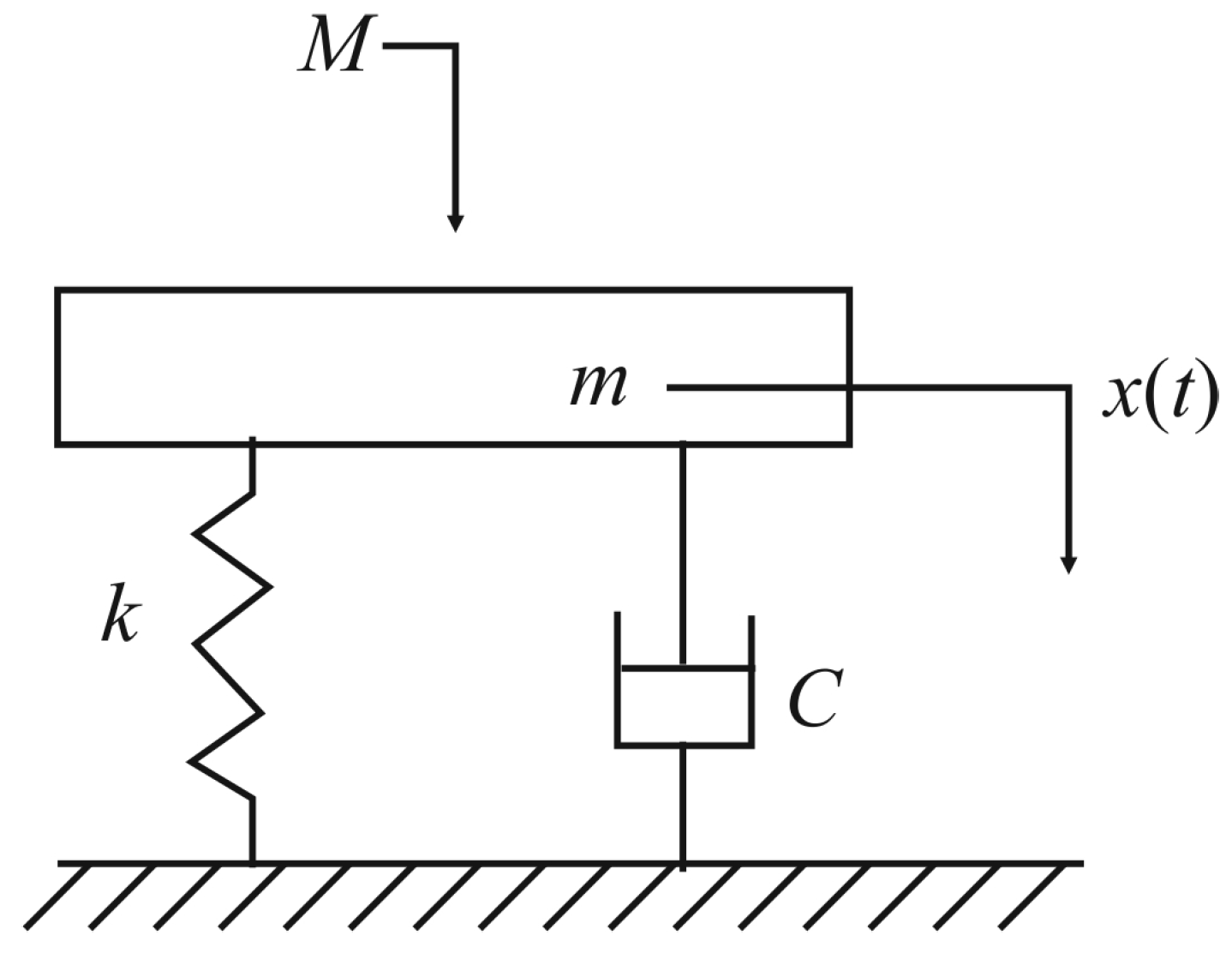
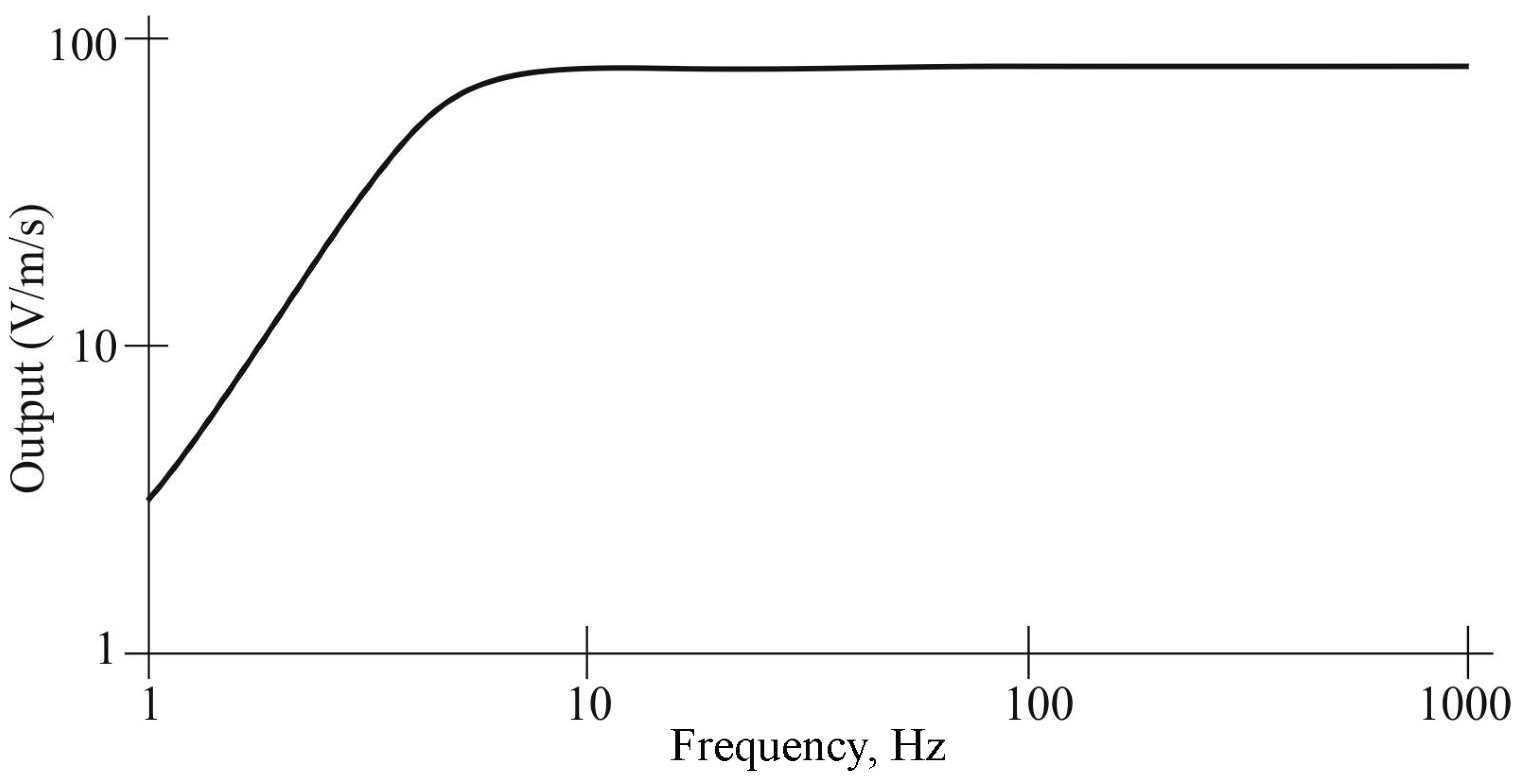
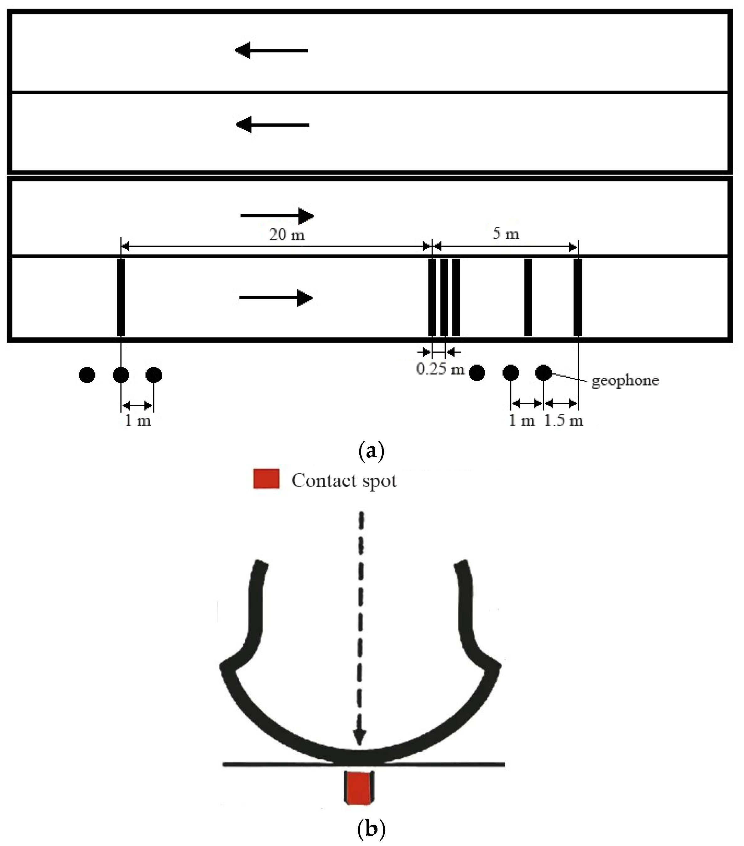
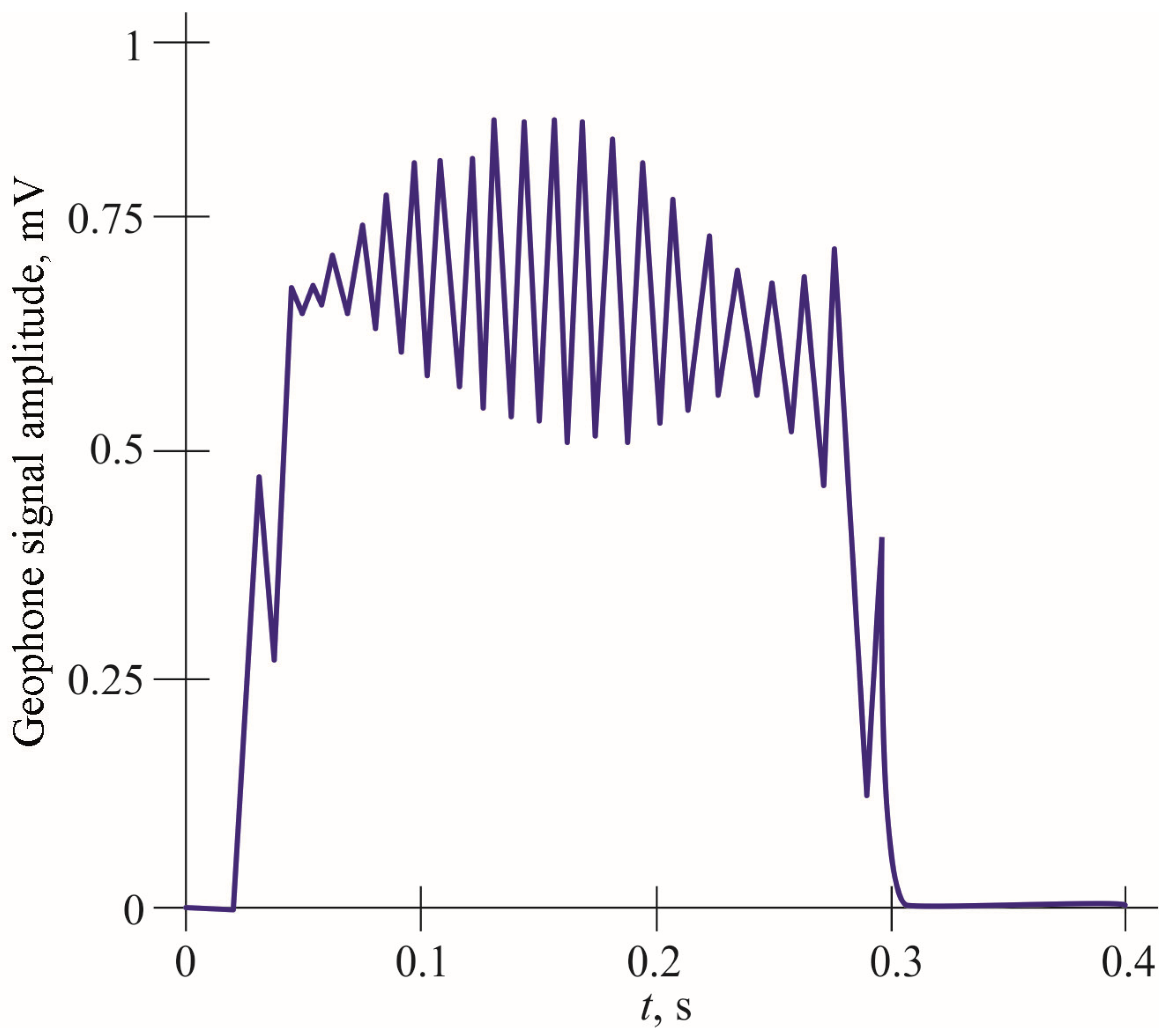
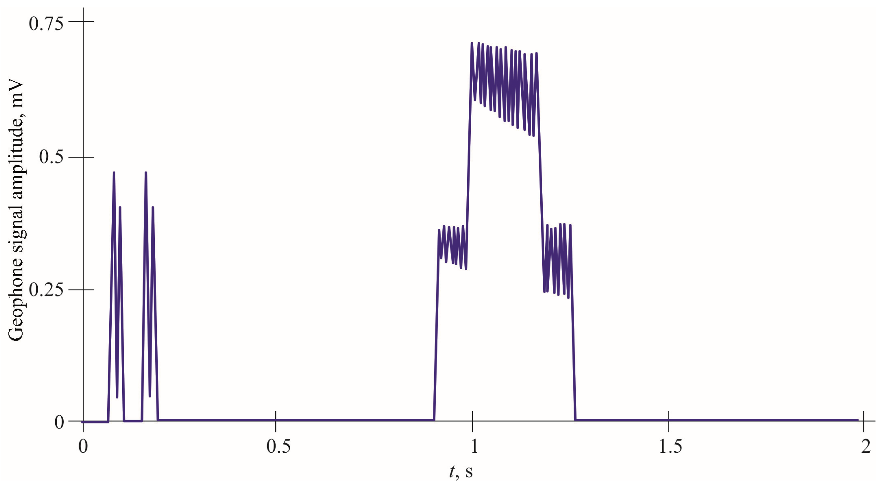
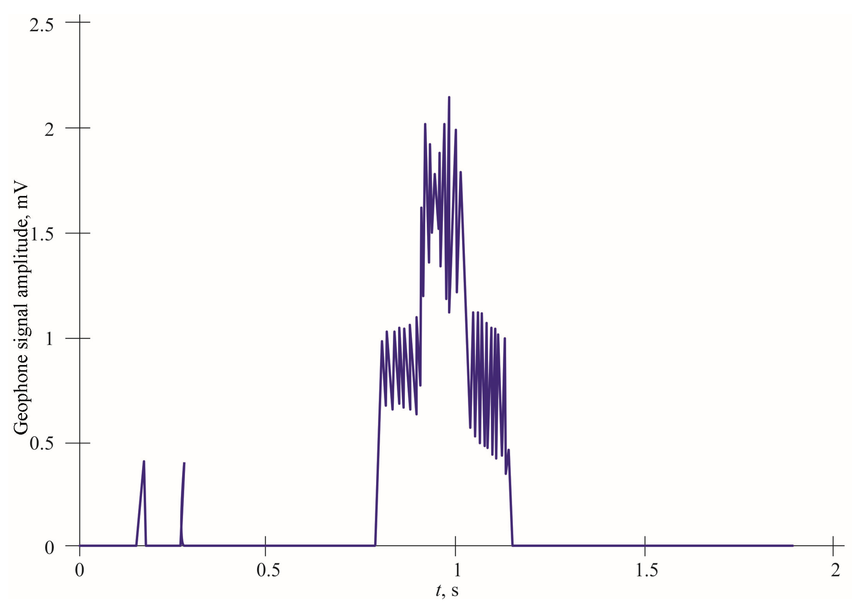
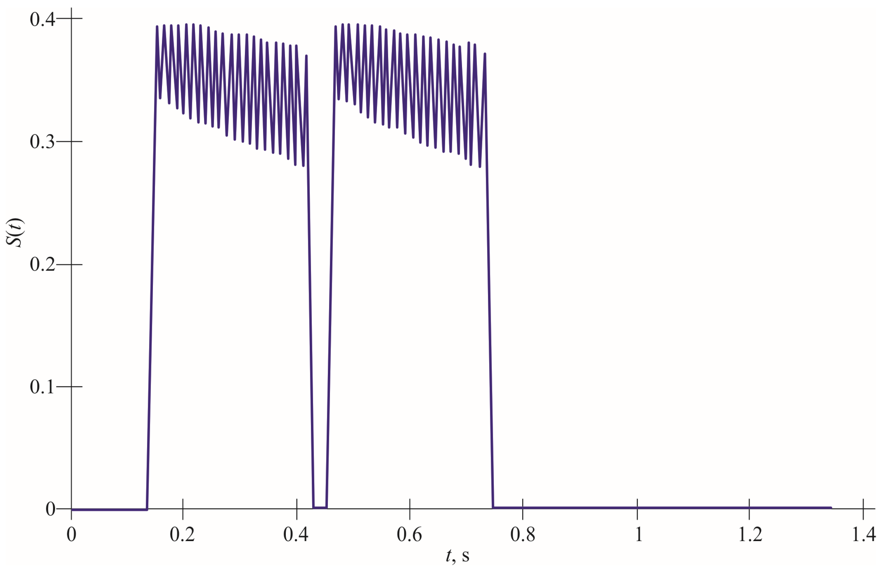
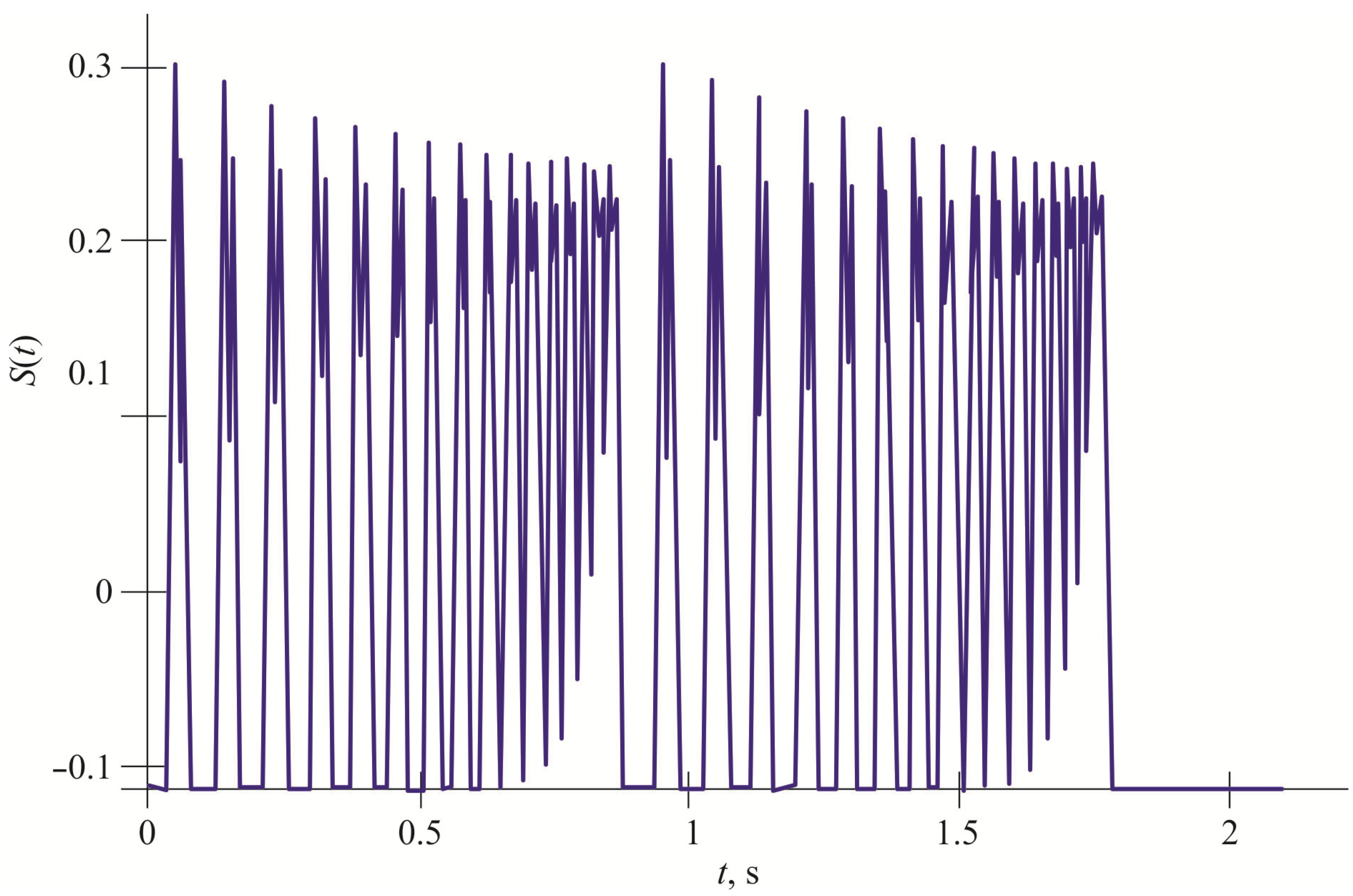
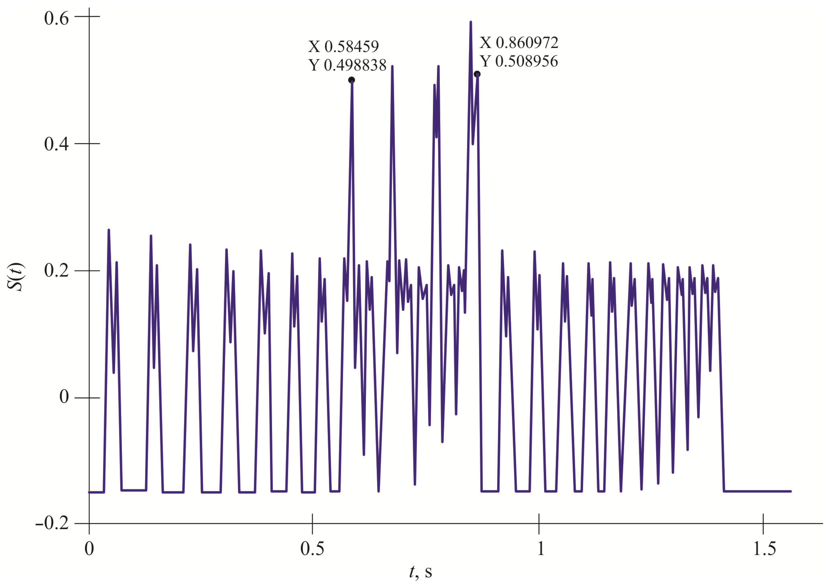
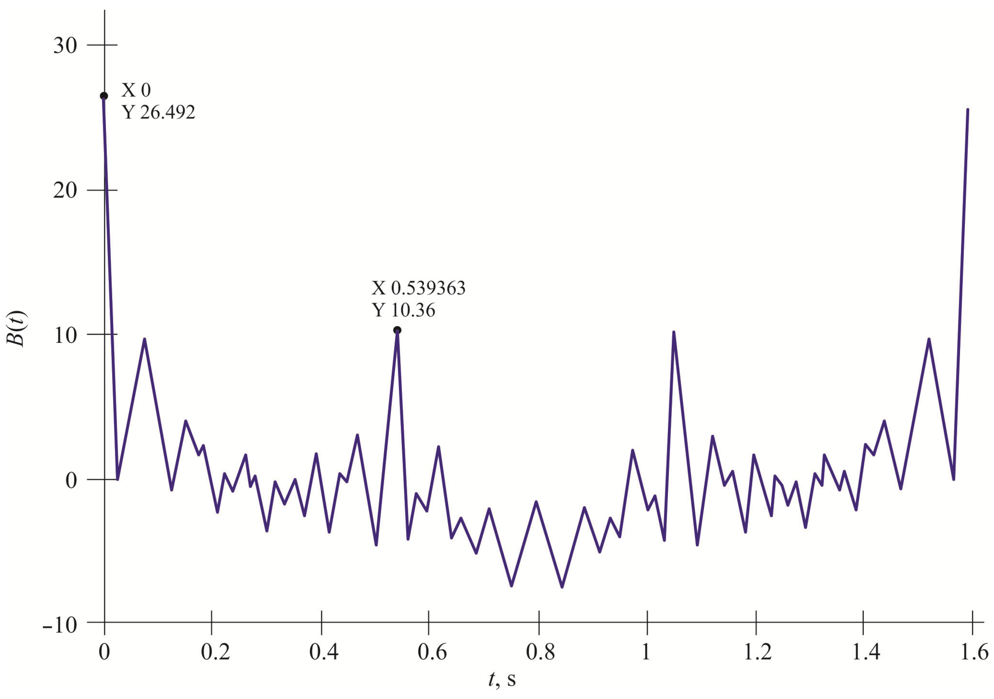
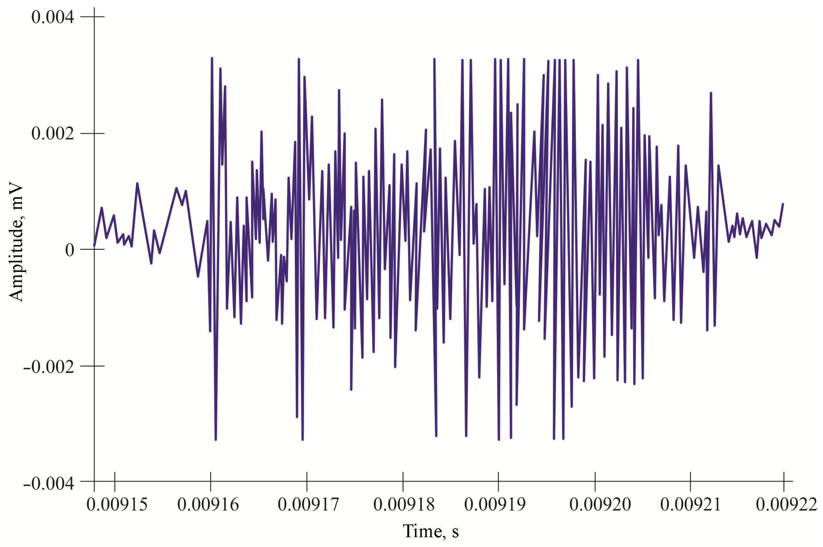
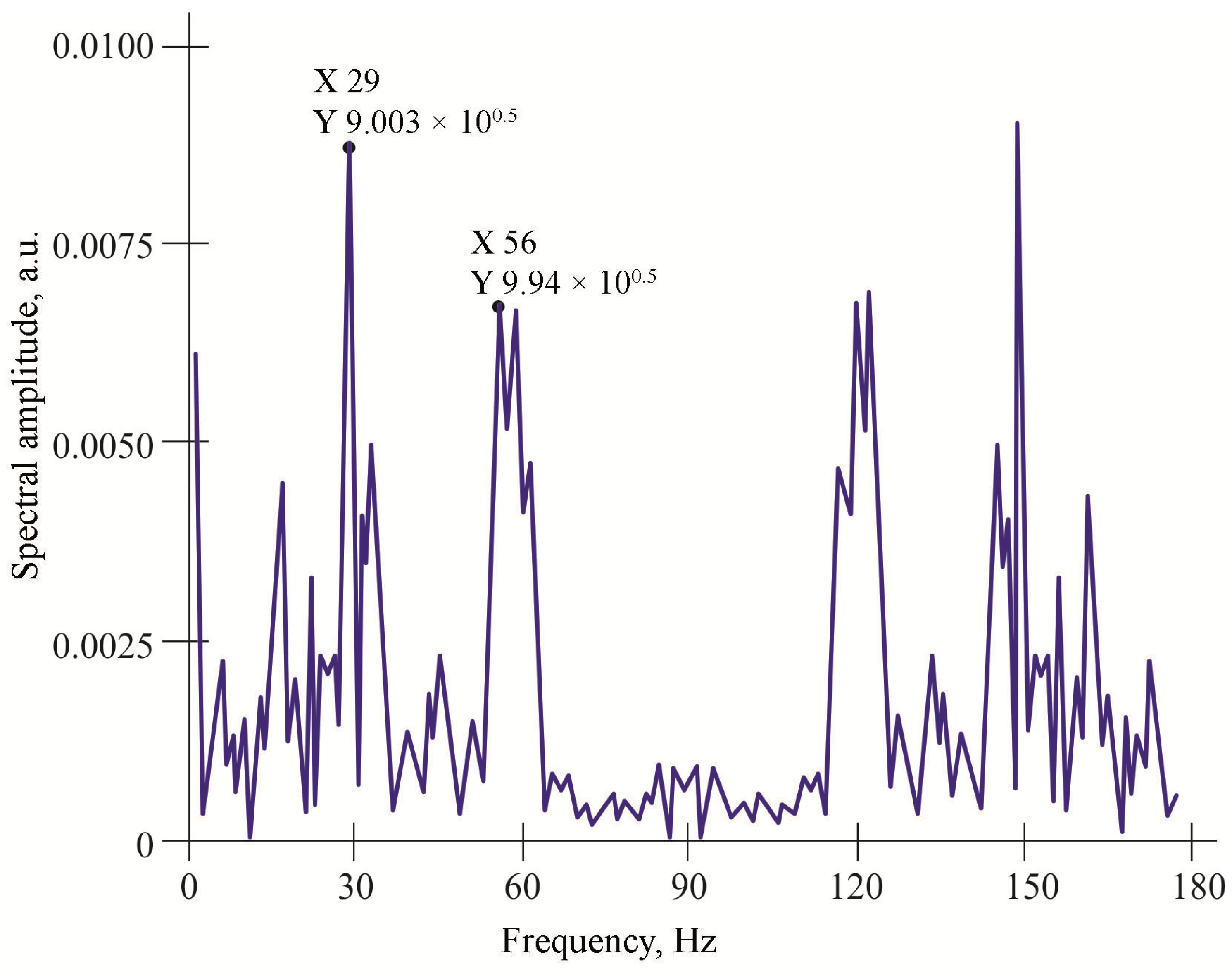
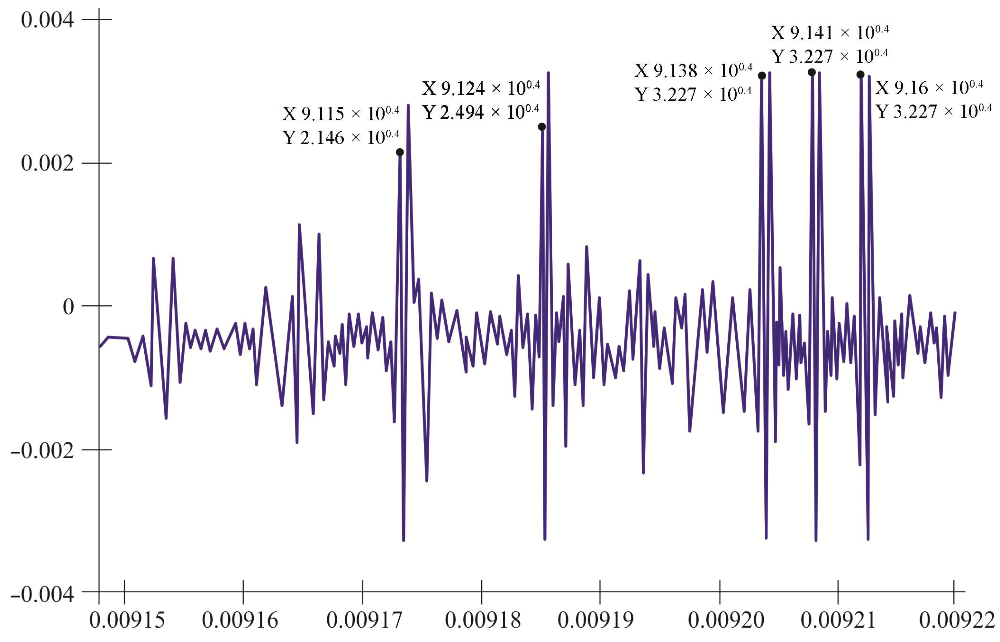