1. Introduction
Buoyancy-induced convection in finite, closed conduits of different shapes has been investigated experimentally as well as theoretically for the last several decades. This interest among researchers mainly reflects the advantage of the use of cooling processes without any aiding external mechanisms in these processes. Further, due to the lower thermal conductivity of traditional or conventional fluids, a significant challenge is posed for cooling the model electronic equipment. The invention of NFs or nanoliquids, which involve a base-fluid and nano-sized particles of oxides or metals, provides a very effective means of replaceing these conventional fluids [
1] to achieve comparatively higher cooling rates. The superior thermal conductivity of NFs has led to many important investigations and produced qualitative as well as quantitative information about the choice of nanoparticle (NP) and the optimal concentration to yield higher thermal transport rates [
2,
3]. Among the various finite-sized conduits, an annular space formed between two co-axial cylindrical-shaped tubes is applied in many important thermal applications, from nuclear reactors to crystal growth design equipment [
4,
5,
6]. Augmentation of the thermal dissipation rate (TDR) by the inclusion of NFs is the major driver behind these investigations.
The thermal management of electronic equipment is one of the fundamental requirements of the electronics industry, the application of which has increased in recent times. To cater to the needs of modern electronic industries, among the several strategies tried by numerous researchers and scientists, attaching a baffle in one or more of the thermally active walls of the enclosure has been found to provide a better way to enhance the thermal transport rates. In this direction, one of the pioneering studies to analyze the impacts of a baffle in a tall tiled rectangular conduit is that of Scozia and Frederick [
7]. The numerical prediction was carried out by considering up to 20 conducting baffles and it was concluded that decreasing the spacing between the baffles or increasing the baffles tends to produce a multi-cellular flow structure and reduction in the overall TDR. For a similar geometrical structure, Facas [
8] reported the impacts of three baffles attached alongside hot and cold boundaries considering three different lengths, and concluded that a longer baffle induces a multi-cellular structure and produces higher TDRs compared to other baffle dimensions. Later, a full-blown analysis of the size and positional influences of a thin baffle on BDC and TDR in a square conduit was performed and it was concluded that an optimum dimension of baffle could be found at which the thermal transport rate could be significantly enhanced compared to non-baffle situations [
9,
10].
Further to the enhancement of TDR shown by fixing baffles to the active boundaries of the conduits, replacing the traditional working fluids by novel NFs was suggested to further improve the heat transfer, with an enhancement in TDR by as much as 10–20 percent demonstrated with use of NFs in [
11]. The impacts of the fin height and NP concentration on the enhancement of TDR were examined by considering two different NPs in a rectangular conduit with longer fins predicted to induce heat transport in [
12]. A 3D mixed convective flow in a perforated heat sink with several cylindrical-shaped fins was quantiatively analyzed by Bakhti and Si-Ameur [
13] considering three NFs. A detailed combined conduction-convection analysis identified that use of Cu NPs induced higher TDR compared to other NPs, and predicted an enhanced frictional effect as well as NF movement with an increase in the Reynolds number. In a 3D triangular conduit, having a stationary as well as a rotating fin, Kolsi et al. [
14] numerically predicted the fin conditions as well as the NP concentration to enhance the TDR. The combined influences of a moving boundary, adiabatic projection at the lower boundary, and an adiabatic baffle on the NF buoyant-flow and associated TDR in a square conduit showed that the energy transport in the chamber could be effectively determined by the dimensions of the adiabatic block as well as the position of the baffle [
15]. Hussein et al. [
16] presented a numerical examination of BDC in a slanted rectangular conduit with a baffle which was filled with two different nanofluids to predict the thermal behavior relative to the baffle dimensions. In many situations, the combined influences of magnetic fields and baffle(s) provide an effective method for controlling convective heat transfer in NF-filled finite geometries, as demonstrated by numerous research studies [
17,
18]. The optimal control of buoyant-assisted convection by utilizing single or multiple baffle(s) in various geometrical shapes, such as cylinders [
19], wavy conduits [
20], and vented domains [
21] has been examined. The choice of the different geometrical configurations in the above studies stems from the necessity to achieve enhanced heat transfer rates, maintain economic viability in production, ensure ease of manufacture, and optimize operational performance.
The utilization of one or multiple baffles in confined NF-filled porous geometries has emerged as a prominent research arena, motivated by the extensive potential engineering applications to improve the thermal efficiency. The porous materials, characterized by their unique structural properties and enhanced thermal transport capabilities, are present in many critical systems, including shell-and-tube heat exchangers, flat-plate solar collectors, and nuclear reactor cooling channels. Recognizing these advantages, researchers have systematically investigated various aspects of porous media and their integration with conductive or non-conductive baffle(s) to achieve optimum heat transfer intensification [
22,
23,
24]. Mahalakshmi et al. [
25] examined the characteristics of MHD mixed convection in a lid-driven porous conduit with a center heater to demonstrate the collective effects of the magnetic force strength, heater orientation, and nanofluid properties on thermal transport performance. The investigation predicted that a horizontal heater arrangement would achieve maximum heat transfer enhancement, and that the magnetic force effectively controls the convective movements within the porous medium. Aly et al. [
26] numerically investigated BDC in a nanofluid-filled porous cavity with different heated fin shapes using a modified ISPH technique. Their analysis revealed that an H-fin shape maximizes the flow circulation rate while a Z-fin shape achieved the highest heat transfer rate. Subsequently, a CFD analysis conducted on magneto-convection in a slanted porous conduit with two conducting fins showed enhanced heat transfer with optimal fin configurations, such as fin space and dimensions, and cavity inclination of
, demonstrating superior performance compared to no-fin configurations [
27].
Recently, porous fins have often been utilized in place of metal fins in thermal applications due to several key advantages, including the enhanced surface area provided by the internal pores, improved fluid mixing through tortuous flow paths, and reduced weight and material costs, among many other advantages [
28,
29]. Further, the incorporation of porous substance within irregular geometric configurations for analyzing buoyancy-driven NF convection represents a significant research domain with multidisciplinary implications, including enhanced geothermal systems, advanced heat exchangers, and microfluidic devices [
30,
31,
32]. The detailed utilization of baffle(s) in controlling BDC flow and associated thermal transport in a variety of geometries filled with diverse NFs, and by considering different constraints, has been reported in comprehensive reviews [
33,
34]. An exhaustive, systematic review of the literature on the implications of various shaped baffle(s) across diverse porous and non-porous NF-filled geometrical configurations reveals a significant research gap. Specifically, the analysis of BDC within baffled porous annular geometries, particularly when integrated with a generalized porous media model and machine learning approaches, remains largely unexplored. Despite the significant industrial and engineering relevance of this configuration, the critical intersection of porous media dynamics, baffle design, and computational methodologies has received insufficient scholarly attention. The current examination addresses this substantial knowledge gap by presenting a comprehensive analysis that bridges traditional fluid dynamics with modern machine learning techniques in the context of baffled NF-saturated porous annular systems.
Despite high-quality outputs from CFD simulations for an individual set of parameters, their inherently high computational cost (which can typically process each simulation case in hours) is often a major obstacle. Running CFD simulations for each new operating condition or design iteration is usually prohibitively expensive in computational time, so a full exploration or fast decision-making becomes out of reach. This is where ML can provide significant potential improvements, taking the shape of powerful surrogate models. Once they have been trained on a representative dataset created by high-fidelity CFD simulations, the ML models can predict the overall performance metrics (e.g., Average Nusselt Number) in a fraction of the time (in many cases, orders of magnitude faster, <0.1 s/prediction). This fast prediction time, even though for an individual point it is less accurate than a full CFD approach, allows for tasks which seemed impossible, such as performing a full exploration of design space to identify new relationships or optimal space, the rapid screening of many design candidates to identify promising designs for more in-depth CFD analysis, or even for use in real-time processes where an instant response is needed. Thus, the ML approach is not meant to replace the ability of CFD for accurate, final validation of some chosen designs; it is instead intended to complement the capabilities of CFD by allowing efficient, large-scale investigation or dynamic applications that are beyond the practical application possibility of direct, iterative CFD simulations.
3. Description of Numerical Methodology
3.1. Finite Difference Methodology
The mathematical modeling of BDC phenomena within the complex nanofluid-saturated porous baffled annular domain poses significant computational difficulties. To address these challenges, our investigation adopts a robust hybrid numerical methodology that combines different finite difference (FD) techniques for a stable and accurate solution. The governing partial differential equations (PDEs) consist of non-linear and coupled vorticity transport, energy balance, and stream function equations. In particular, the vorticity-transport equation incorporates Darcy–Forchheimer–Brinkman terms to account for porous media effects, and additional terms to model the modified thermophysical properties of NF. Further, the baffled annular configuration also introduces additional complexities through the boundary conditions at the baffle interfaces.
Our solution methodology employs a domain discretization using a uniform grid across the entire annular region and special care has been taken while assigning grids along the baffle. For the temporal and spatial discretization, we adopt the following FD approximations:
Temporal Derivative: Forward difference quotients are implemented for all time-dependent terms, resulting in first-order accuracy in time ().
Spatial Derivatives: Central difference schemes are utilized for spatial derivatives, providing second-order accuracy ( and ) in the computational domain.
The solution methodology strategically integrates two different numerical techniques:
Alternating-Direction Implicit (ADI) Procedure: The parabolic nature of the vorticity and energy transport equations has been integrated by a two-step ADI scheme. In the first half-time step, the FD equations are solved implicitly in the R-direction while treating the Z-direction terms explicitly. In the second half-time step, the process is reversed, ensuring unconditional stability while maintaining computational efficiency.
Successive Line Over-Relaxation (SLOR): The elliptic stream function equation is solved using SLOR, where each grid line is solved implicitly while sweeping through the domain. An optimal over-relaxation parameter () between 1.0 and 2.0 was dynamically adjusted to accelerate convergence based on the control parameters of the chosen problem.
The FD discretization process transforms the PDEs into systems of linear algebraic equations with tri-diagonal coefficient matrices. These systems are efficiently solved using the popular Thomas algorithm (tri-diagonal matrix algorithm or TDMA), which provides direct solutions.
The iterative solution process employs dual convergence criteria for transient as well as stationary cases:
For transient PDEs, iterations are carried out until: , where represents either vorticity or temperature, and is a predefined temporal tolerance, typically set at .
For the stream-function equation, spatial convergence is achieved when: , where k denotes the special iteration level and is the spatial tolerance, typically set at .
An in-house code in ForTran was developed to systematically invert the system of equations arising from the different model equations. The algorithm implementation follows a sequential approach where the energy and vorticity equations are advanced in time, followed by stream function updates and velocity-stream function relations at each time step, ensuring proper coupling between the momentum and energy transport mechanisms in the complex NF-saturated porous annular domain. Before the simulations, a systematic and proper grid independence trial was conducted by choosing coarse to fine grids from
to
and an optimum grid structure was chosen based on the solution accuracy and computational time. For choosing the optimal grid size, we identified the average
and
as the sensitive measure to decide the appropriate grid size. Based on these careful experiments, we found a grid size of
satisfactorily provided the accurate predictions as compared to the other grid sizes. However, the details pertaining to the grid independence tests are not provided here for brevity, but can be found in our recent studies [
5,
35,
36].
3.2. Validation
To validate the current simulation outcomes, in this section, we report several important trial simulations to compare, qualitatively as well as quantitatively, with standard benchmark predictions existing in the literature, which are illustrated through
Table 3 and contour illustrations (
Figure 2), to support the credibility of the in-house developed code. In this regard, first, we modified our code with uniform heating and cooling, without the presence of a baffle (
), for a uniformly heated-cooled non-baffled annulus and square geometry. We performed simulations for a thermal-buoyancy-assisted convection and obtained the thermal transport rates for an annular geometry without baffle
to compare with the quantitative predictions of Abouali and Falahatpishesh [
4]. Our predictions in the annular conduit for different magnitudes of
and
are found to be in fair agreement with the numerical outcomes of Abouali and Falahatpishesh [
4], as displayed in
Table 3, with minimum allowable deviations.
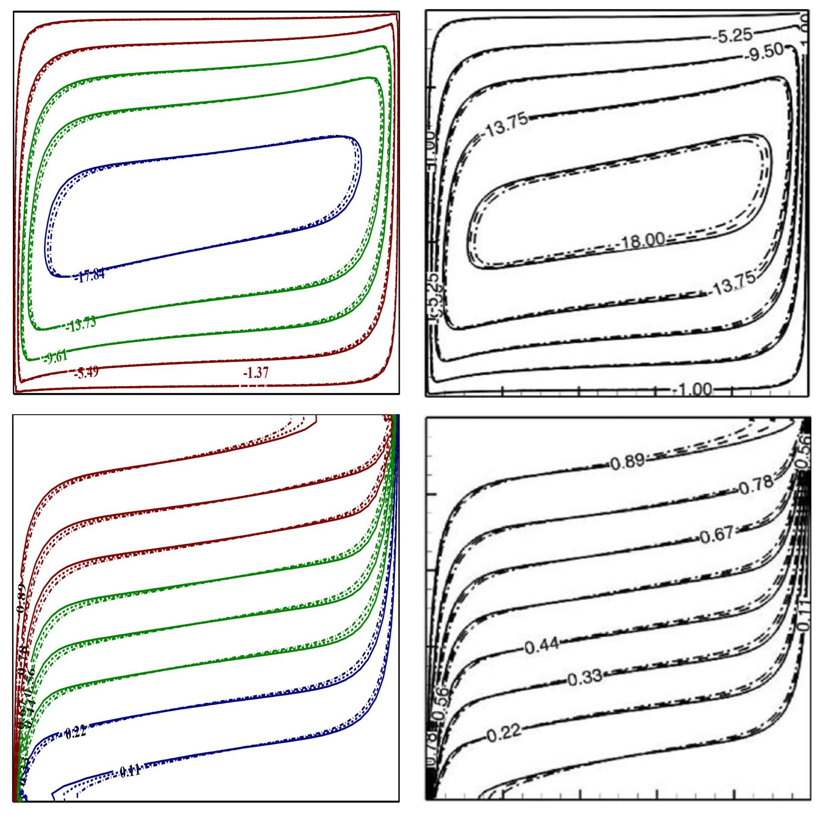
Furthermore, in another comparison with a square geometry, we performed additional simulations, by putting
, to mimic the contour simulations of Nguyen et al. [
2] for a square geometry containing Cu-H
2O NF, and present the same in
Figure 2. The comparative predictions of the streamlines and isotherms vividly reveal the excellent similarity between our simulations and the predictions of Nguyen et al. [
2] for two different NP concentrations. These qualitative and quantitative validations with systematic grid independence tests ensure the authenticity of our in-house code and provide confidence to perform further simulations in this investigation.
3.3. Proposed Machine Learning Methodology
The proposed methodology outlined in this study investigates whether machine learning techniques can be used to predict the mean Nusselt number, a critical indicator of heat transfer performance, within a cylindrical annular domain. This approach employs a thorough data-driven pipeline consisting of data analysis and preprocessing, model training, hyperparameter tuning, and model validation. We use a conventional machine-learning algorithms in addition to a deep learner that relates the dependent variables (e.g., Rayleigh number, baffle length, etc.) to the predictee. The primary motivation for this is to develop reliable and accurate predictive models to support thermal equipment designers.
The preprocessing step is essential for maintaining the quality of data and readiness for model training. Our first step is exploratory data analysis to develop an understanding of individual feature distributions, potential outliers, and correlations across features. The dataset also contains missing values, and therefore, we impute for missing values. Next, we standardize the data to have a mean of zero and a variance of one. This step is important because it helps ensure that features with larger magnitudes do not dominate the learning process, especially with distance-based algorithms and neural networks. Lastly, a train–test split is completed to separate the dataset into independent train and test datasets which is crucial to create an unbiased evaluation of model generalization performance.
We utilized a range of machine learning models to predict the mean Nusselt number. This list of models includes ensemble models such as Random Forest and Gradient Boosting, known for their robustness to complexities and ability to capture non-linearities. A Support Vector Regressor (SVR) is also considered as it allows flexibility in modeling different kinds of relationships through kernel functions. Additionally, we implement a Ridge Regression model as a baseline linear model to compare against the more complex models. Finally, we developed an Artificial Neural Network (ANN) to test the capabilities of deep learning.
Hyperparameter optimization is conducted for each model to maximize performance. Instead of an exhaustive grid search, we opted for a randomized search. This method still allows for exploration of the hyperparameter space by choosing a fixed number of hyperparameter combinations to sample. This method represents a good trade-off of computational cost and probability of finding near-optimal hyperparameters. A repeated k-fold cross-validation is also used for model hyper-parameter tuning to provide a robust estimate of model performance and counteract overfitting to the training data.
Model performance is evaluated using a comprehensive suite of metrics, including R-squared (R2), Root Mean Squared Error (RMSE), Mean Absolute Error (MAE), and Mean Absolute Percentage Error (MAPE). These metrics are defined as follows, where represents the true value, represents the predicted value, and n is the number of samples:
R-squared (R2): Measures the proportion of variance in the dependent variable that is predictable from the independent variables. A value of 1 indicates a perfect fit.
where
is the mean of the true values.
Root Mean Squared Error (RMSE): Represents the square root of the average squared difference between the predicted and actual values. Lower values indicate better fit.
Mean Absolute Error (MAE): Represents the average absolute difference between the predicted and actual values. Lower values indicate better fit.
Mean Absolute Percentage Error (MAPE): Represents the average absolute percentage difference between the predicted and actual values. Lower values are better, with 0% indicating a perfect fit.
These evaluation metrics each provide different insights about different aspects of model accuracy. In addition to these metrics, we also look at the residuals in order to evaluate the stated assumptions of the model and examine any systematic biases. The best overall model is determined by sufficient overall performance against these metrics, with emphasis on generalization ability on the hold-out test set.
The proposed methodology is summarized in Algorithm 1,
Predict Nusselt Number, which outlines the complete workflow for predicting the average Nusselt number. It begins with data analysis and preprocessing, including splitting the data into training and testing sets and applying a preprocessing pipeline for imputation and scaling. The core of the algorithm involves iterating through a set of predefined models, including both traditional machine learning algorithms and an Artificial Neural Network (ANN). For each model, hyperparameter optimization is performed using randomized search with cross-validation, except for the ANN, which is trained with techniques like early stopping.
| Algorithm 1 Predicting average Nusselt number |
- 1:
Input: Dataset , where is a feature vector and is the Nusselt number. - 2:
Output: Best predictive model , evaluation metrics. - 3:
procedure PredictNusseltNumber(D) - 4:
▹ Copy for analysis - 5:
Perform data analysis on (histograms, correlation matrix, etc.) - 6:
Separate features (X) and target (Y) from D - 7:
Split into training and testing sets (e.g., 80/20 split) - 8:
Create preprocessing pipeline (imputation, scaling) - 9:
- 10:
- 11:
{RandomForest, GradientBoosting, SVR, Ridge, ANN} - 12:
- 13:
- 14:
for do - 15:
if M is ANN then - 16:
Define ANN architecture (layers, activation functions, etc.) - 17:
Compile ANN model (optimizer, loss function) - 18:
Train ANN with cross-validation, early stopping, and learning rate scheduling - 19:
Trained ANN - 20:
else - 21:
Define hyperparameter search space for M - 22:
Perform randomized search with cross-validation to find best hyperparameters - 23:
Model M with best hyperparameters - 24:
end if - 25:
Evaluate on and - 26:
Store evaluation metrics (R2, RMSE, MAE, MAPE) in - 27:
end for - 28:
Select best model based on evaluation metrics (e.g., lowest MAE on test set) - 29:
return , - 30:
end procedure
|
Algorithm 1 then evaluates each trained model on both the training and testing sets, storing the results. Finally, it selects the best-performing model based on a chosen evaluation metric (e.g., MAE on the test set) and returns this model along with the comprehensive evaluation results for all models. This structured approach ensures a rigorous and reproducible methodology for model development and selection.
3.4. Implementation Details
The developed ML models are proposed to predict the Average Nusselt Number (). The used dataset was split into a training set, 80% of the samples, and a test set, 20% of the samples. The splitting of the data was completed using the scikit-learn train_test_split function. Then, a preprocessing stage was executed, where all input features were standardized using scikit-learn’s StandardScaler. For those models that were developed rather than the neural network-based model, namely, Random Forest, Gradient Boosting, SVR, and Ridge Regression, a hyperparameter search was conducted using RandomizedSearchCV provided by scikit-learn. RandomizedSearchCV evaluates a prespecified set of hyperparameter values for each model, on the training dataset (employing a 5-fold cross-validation). The goal was to determine a set of hyperparameter values that maximized the score. The key hyperparameters that were tuned included n_estimators, max_depth for the various ensemble-based models, learning_rate for GradientBoosting, C, and kernel type for SVR, and for the regularization strength in the Ridge Regression.
The proposed ANN architecture was constructed as a sequential multi-layer perceptron model with the TensorFlow Keras API. The architecture consisted of an input layer with three hidden dense layers (e.g., consisting of 128, 64, and 32 neurons, respectively) with 1 dense output layer with a linear activation function for the regression problem. The activation function in the hidden layers was the ReLU (Rectified Linear Unit). To reduce overfitting, the model had regularization applied to the weights of the hidden layers, batch normalization following the hidden dense model, and dropouts (e.g., with 0.2 probability rate) between the hidden dense layers. The ANN model was compiled with an initial learning rate of the Adam optimizer, with the goal of minimizing the mean squared error. Training had a predetermined upper limit for the epoch (i.e., 500 maximum epochs) and employed a count to the batch size of the training samples.
4. Results and Discussion
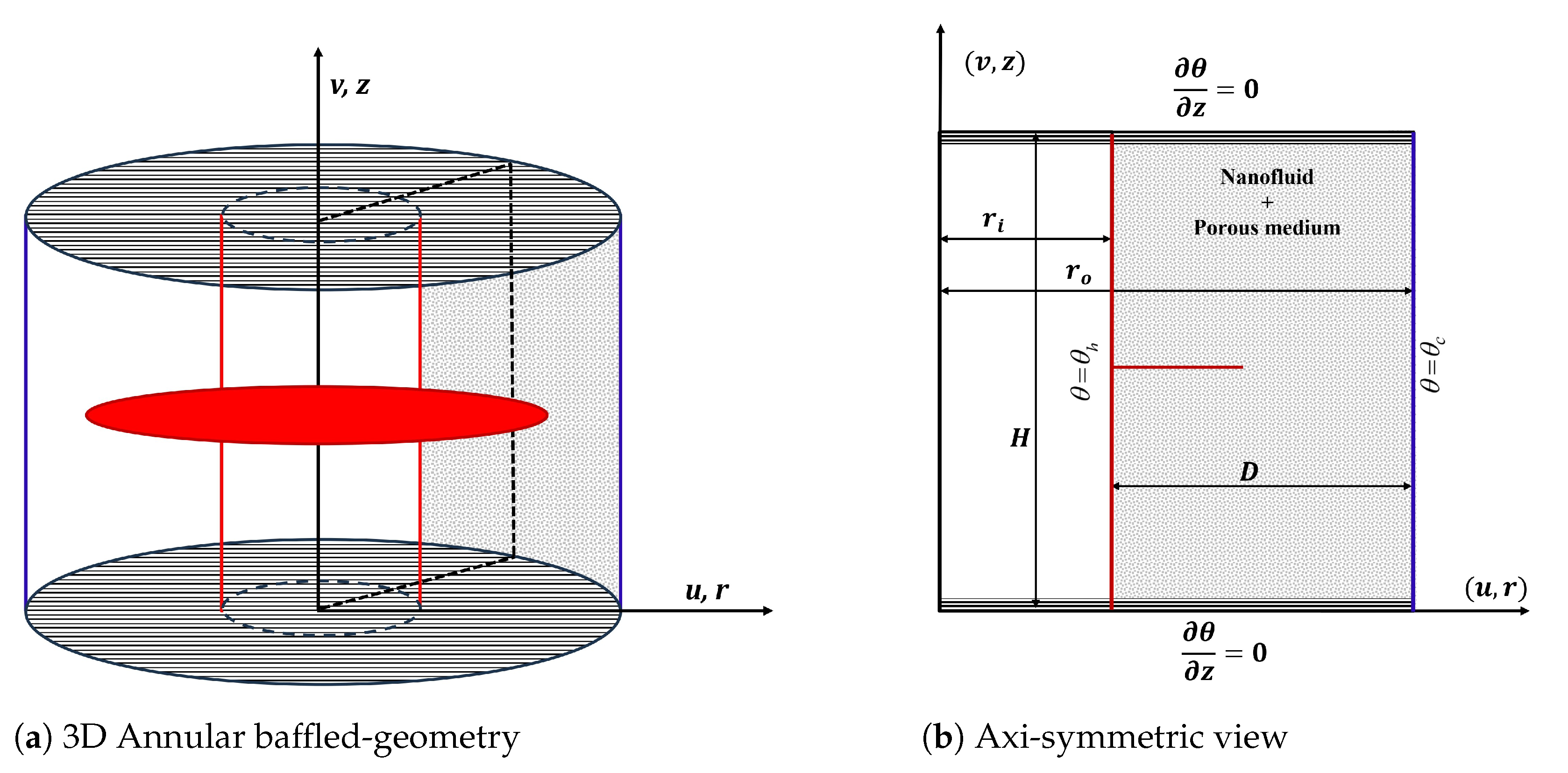
The current analysis involves nine dimensionless parameters, namely, the Rayleigh , Darcy , and Prandtl numbers, the baffle length and location , porosity , NP concentration , aspect and radii ratios, and a full-blown parametric study along with ANN modeling, which would be a formidable task. Hence, in our analysis, the parameters, and are fixed at , and 2, respectively. However, the ranges of the other parameters are as follows: , , , , . These parametric ranges would highlight the weaker, meager, and stronger impacts of all pertinent parameters on the qualitative as well as quantitative predictions.
4.1. CFD Simulation Results
4.1.1. Impact of Control Parameters on Flow and Thermal Contours
In the streamline contour graphs, the positive and negative values have important physical meanings. The positive streamlines indicate counterclockwise rotation of fluid, representing the fluid motion in the counterclockwise direction. However, the negative streamlines refer to clockwise circulation of fluid, indicating fluid movement along the clockwise direction.
The flow and thermal contours depicted in
Figure 3 illustrate the significant influence of
on the flow and thermal characteristics within the annular domain (the arrows in the streamline plots highlight the direction of the vortex rotation in the annulus). At
, the flow exhibits a single primary circulation vortex with relatively symmetric and organized patterns, suggesting a conduction-dominated thermal transport regime. The isotherms at this lower
appear nearly vertical with minimal distortion, further confirming the dominance of conductive heat transfer. The presence of a baffle introduces only minor perturbations in both flow and thermal distributions, while maintaining the overall stability of the system. In contrast, at
, the flow structure undergoes a substantial transformation. The streamlines reveal the formation of multiple circulation cells with significantly higher flow intensities, evidenced by the densely packed streamline contours. The flow field exhibits pronounced distortion near the baffle, indicating strong convective currents. The corresponding isotherms at this higher
display substantial distortion and clustering, particularly near the walls and baffle, resulting in the formation of distinct thermal boundary layers and enhanced temperature stratification in the core region. This behavior clearly signifies the transition to a convection-dominated heat transfer regime. The comparison between base-fluid (
, continuous curves) and NF (
, dotted curves) reveals subtle yet important differences in both flow and thermal characteristics. Although the overall flow structure basically remains similar, the presence of NPs modifies the flow patterns and enhances the heat transfer characteristics. This enhancement is particularly evident in the high
case, where the NF demonstrates improved thermal mixing and heat transfer capabilities.
The analysis of the
influence on the flow features and thermal patterns reveals compelling insights into porous material behavior, as illustrated in
Figure 4. At a higher Darcy number
, manifesting enhanced permeability, the NF flow exhibits complex patterns characterized by dual circulation cells and pronounced flow distortions, particularly near the boundary regions. The corresponding isotherm contours exhibit strong clustering, indicating the presence of steep thermal gradients across the domain. The impact of different porosities (
and
) becomes significant at this higher Darcy number, with higher porosity resulting in more intense circulation patterns. In contrast, at a lower Darcy number
, indicating reduced permeability, the flow structure shows simpler patterns, characterized by a single primary circulation vortex, and the thermal distribution shows a higher uniform spacing and smoother transitions. The influence of porosity variation becomes less pronounced at this lower Darcy number, indicating that permeability effects play a dominant role over porosity impacts. The influence of the baffle dimensions
and locations
on the flow and thermal patterns within the porous annular region is reported in
Figure 5. Four distinct baffle configurations are analyzed, characterized by varying different combinations of
L and
dimensions. For the case of
, denoting a shorter baffle positioned closer to the bottom, the flow field exhibits a primary circulation pattern with densely positioned streamlines, while the isotherms show moderate thermal stratification. However, for
but increasing
to
(shifting the baffle to a higher location), a notable alteration in the flow structure occurs with a more pronounced distortion in the streamlines adjacent to the baffle region, accompanied by enhanced thermal mixing, as evidenced by the isothermal patterns. For configurations with longer baffles
, the flow and thermal characteristics exhibit larger significant variations. At
, the extended baffle creates a more restricted flow passage, causing strong flow circulation rates in the restricted region and more pronounced thermal gradients. The case of
shows intense flow modification, with different flow separation and recirculation zones, along with sharp thermal gradients, particularly near the baffle edge.
4.1.2. Impact of Control Parameters on Thermal Transport Rates
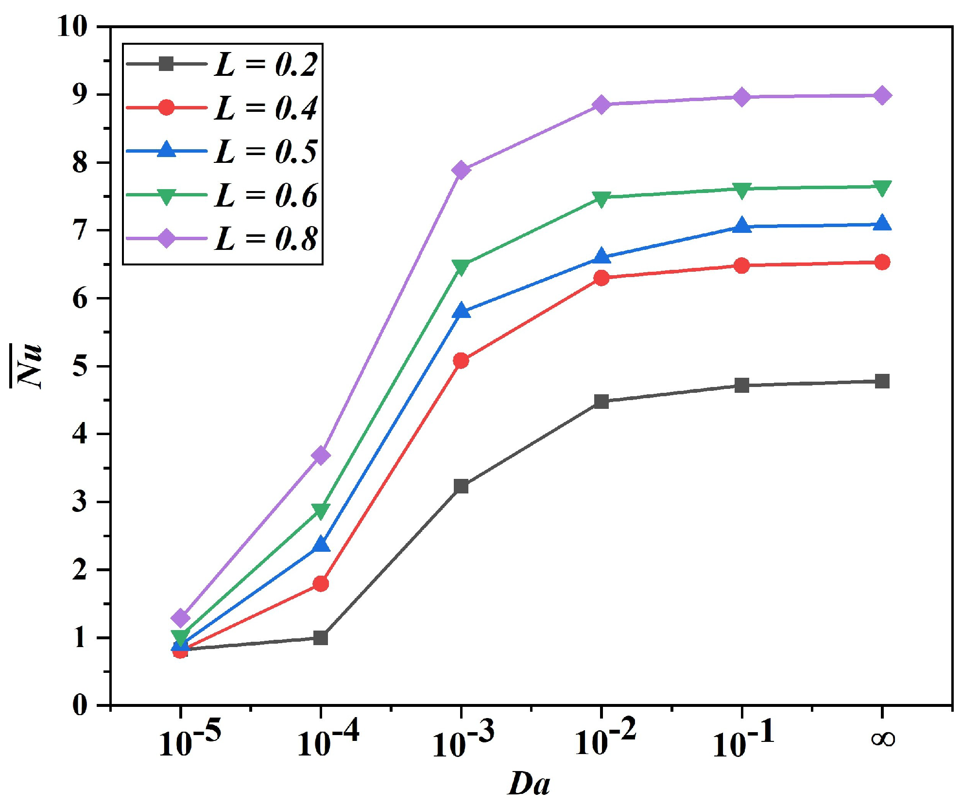
Figure 6 illustrates the thermal efficiency relationship between the average
and the Darcy number for various fin positions
. The thermal performance predicts a clear physical trend, indicating at low Darcy numbers (
) that the flow drag is severe, and the heat transfer is primarily conduction-dominated, resulting in low
across all fin positions. As the
increases, particularly between
and
, a drastic enhancement in heat transfer due to stronger convective effects occurs. The fin position closer to the bottom
consistently records superior thermal performance, achieving a maximum Nusselt number. This superiority can be attributed to better utilization of the buoyancy-driven flow, as the lower fin position allows for more effective development of thermal boundary layers and convective currents. Conversely, higher fin positions
show reduced thermal efficiency, suggesting that placing the fin at higher locations impedes the BDC flow pattern. The variation in the average
curves indicates that further increase in permeability beyond
produces minor variations in heat transfer enhancement. The interplay between the baffle dimension (
) and Darcy number (
) on heat transfer effectiveness is reported in
Figure 7. An overview of the predictions suggests that shorter fins (
) consistently outperform longer ones, achieving the highest thermal transfer (
). This superior performance of shorter fins could be attributed to reduced flow blockage, as seen in a longer baffle, permitting better fluid circulation and hence enhanced convective thermal transport. As the baffle dimension increases to
, the thermal performance deteriorates due to higher flow resistance, which leads to reduced convective mixing. The influence of permeability (
) follows a characteristic pattern. At low
(
), conduction dominates and heat transfer is minimal across all fin lengths. A sharp enhancement in thermal transport occurs between
and
, marking the transition from conduction- to convection-dominated regimes. Beyond
, the variation in the curves stabilizes, suggesting that further increases in permeability provide minimal thermal benefits.
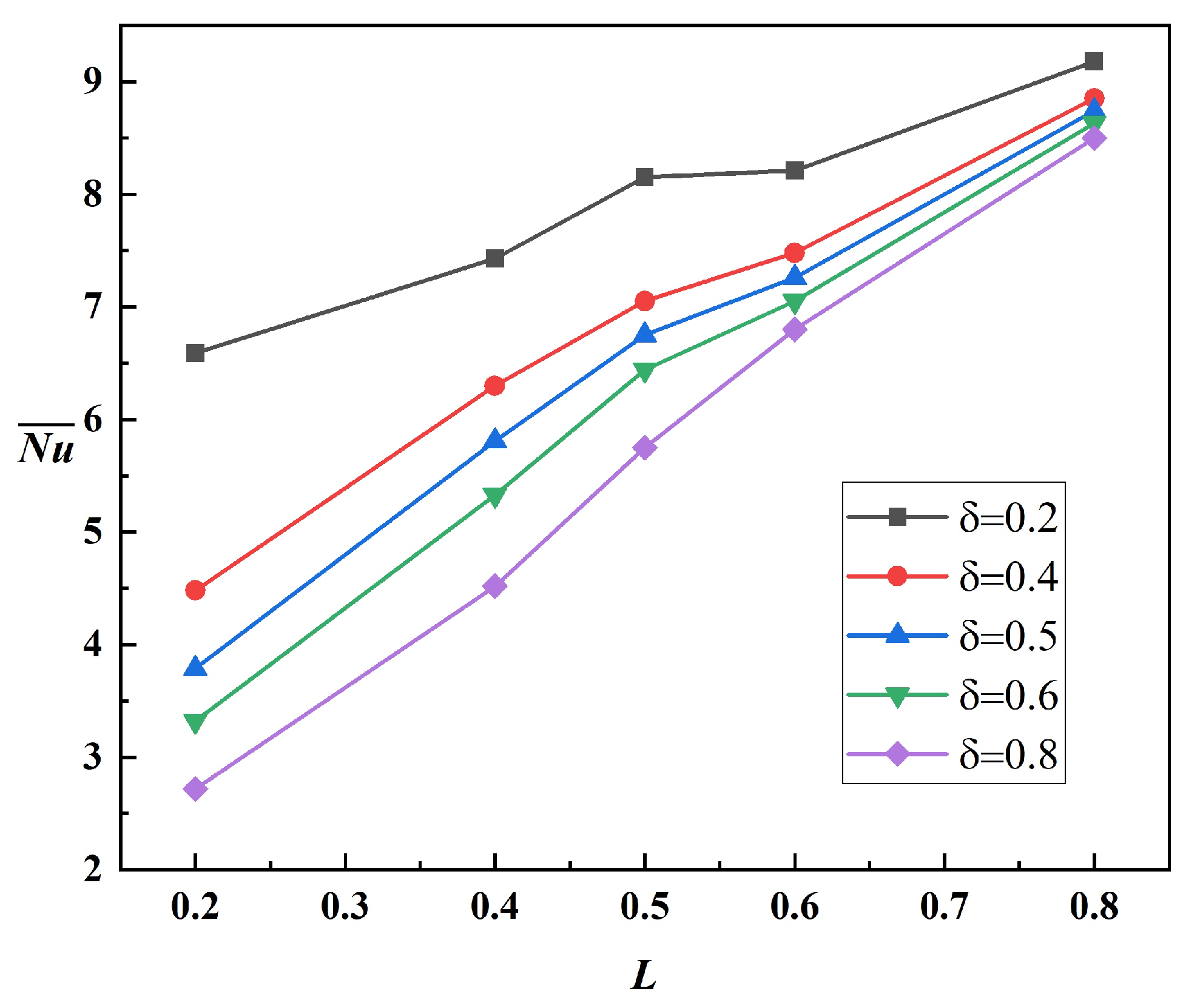
Figure 8 demonstrates the collective impacts of the fin length (
) and position (
L) on the thermal efficiency for the fixed parameters (
,
,
,
). For the combinations of shorter fins (
) and lowered positions (
), the heat transfer performance is predicted to be superior, with
around
. However, as the baffle position increases to
, an increase of
in the average
could be achieved. In addition, it could be observed that the performance differences between various fin dimensions become less pronounced, with all curves converging to Nusselt numbers around 8.5–9 for the elevated baffle location (
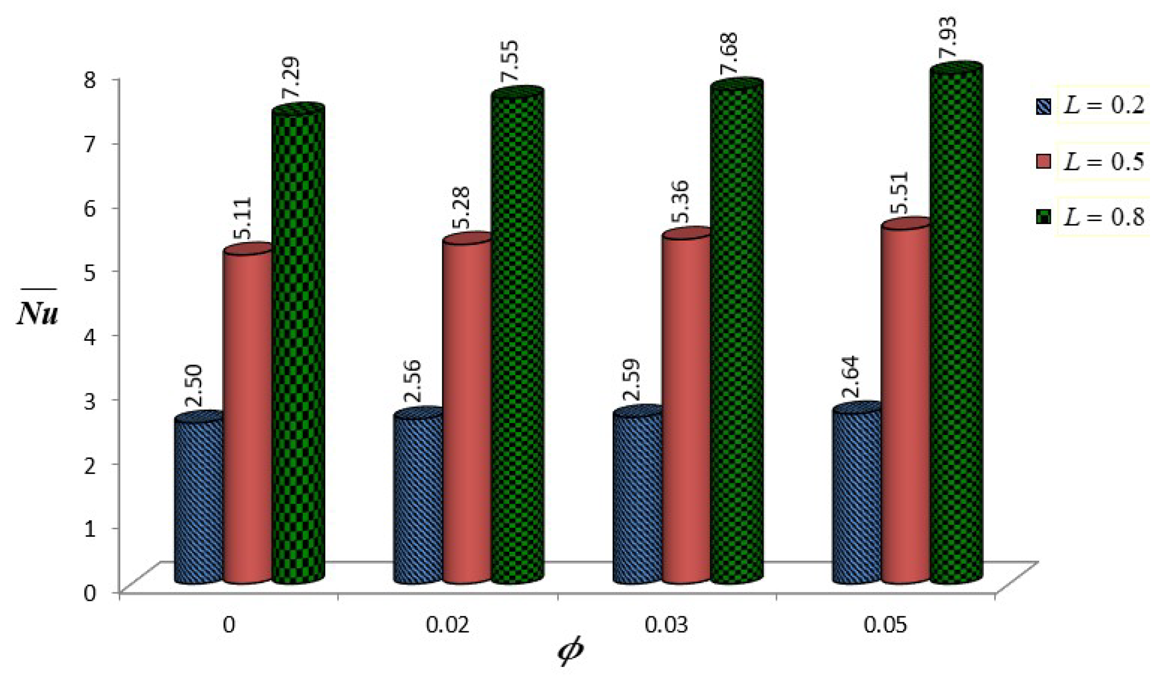
). The lower fin lengths consistently outperform larger dimensional baffles across all fin locations, attributed to better utilization of the developing thermal boundary layer and convective currents near the bottom portion of annular domain. The effects of the NP volume fraction (
) and fin length (
) on thermal transport performance are reported in the bar graph (
Figure 9) at
,
,
, and
. The parametric analysis elucidates that shorter fins (
) consistently demonstrate superior thermal transport, with Nusselt numbers ranging from
to
across all NP concentrations. A moderate increase in heat transfer is observed with an increasing NP volume fraction, particularly for
, where
increases from
(
) to
(
). However, this enhancement becomes less pronounced for longer fins (
), where
values remain relatively lower (around 4.2–4.5). To consolidate the outcomes from these predictions, it may be suggested that the combination of shorter baffles with high-density NPs could enhance the thermal transport among other combinations.
Figure 10 reports the combined influences of the NP volume fraction (
) and fin location (
L) on the thermal transfer characteristics at
,
,
, and
. Fins positioned at
exhibit significantly enhanced heat transfer, with Nusselt numbers ranging from
to
across all NP concentrations. The addition of NPs shows a modest positive impact on heat transport, with the most pronounced enhancement observed for
, where
increases from
(
) to
(
). However, fins positioned closer to the upper portion of the annular domain (
) demonstrate consistently lower heat transfer rates (
), suggesting that positioning fins too close to the upper boundary restricts fluid circulation and thermal mixing. The intermediate fin position (
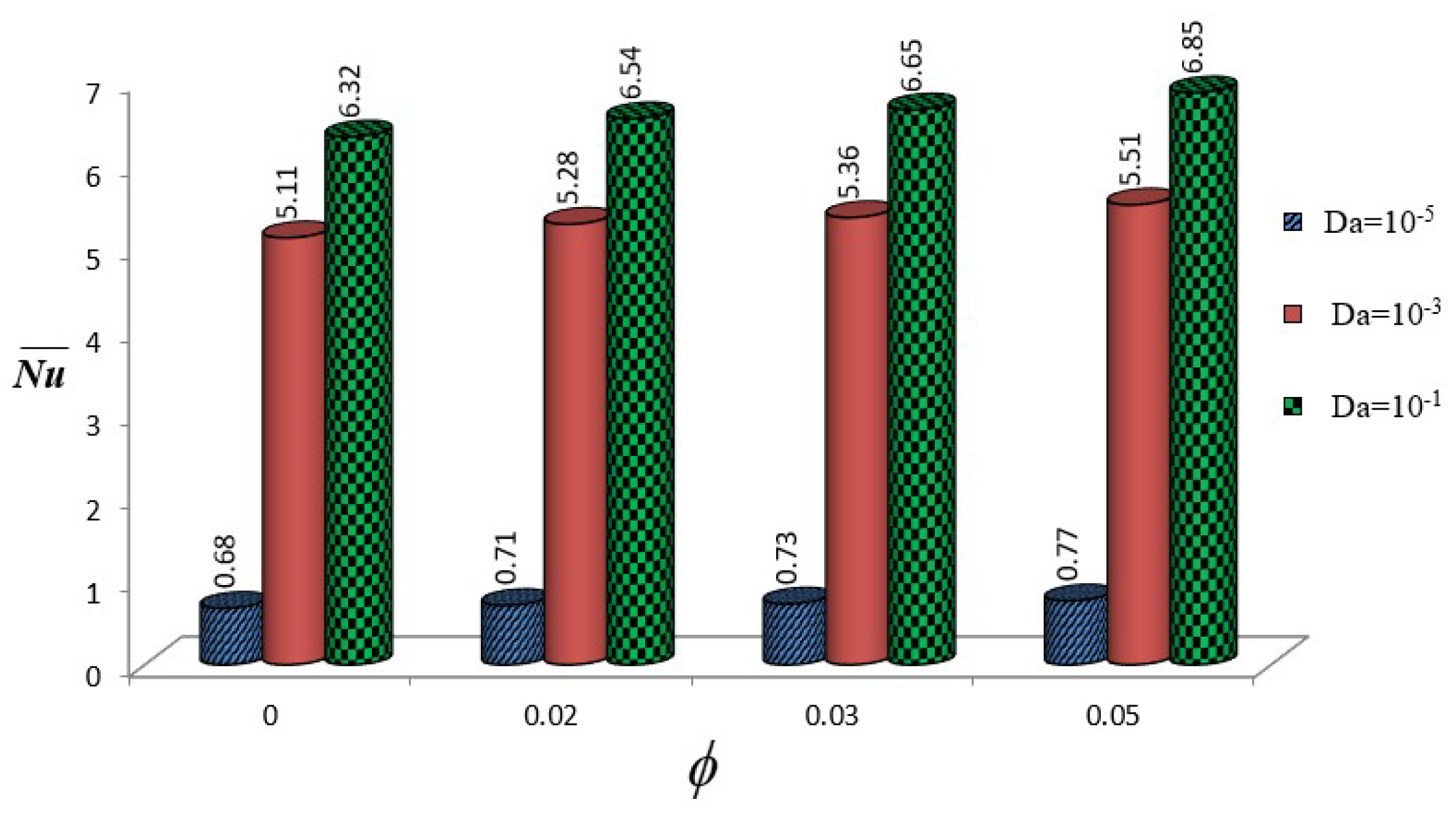
) shows moderate performance, indicating optimal baffle placement is crucial for maximizing the combined benefits of fin-enhanced heat transfer and NF properties. The numerical predictions in
Figure 11 demonstrate the interplay between
and
on thermal efficiency at
and
. As expected, higher magnitude of
(
) yields substantially enhanced thermal transport rates, with average
ranging from
to
, indicating augmented fluid permeability and consequently, higher convective transport. A moderate increment in the heat transport is observed with an increase in NP concentration across all Darcy numbers. However, for the low permeability case, (
), the thermal transfer remains notably suppressed (
despite increasing NP concentration, suggesting that the flow constriction dominates over the enhanced thermal conductivity impacts of NPs. The intermediate permeability case (
) shows moderate heat transfer enhancement, highlighting the critical role of porous media permeability in determining the effectiveness of NP addition.
4.2. Machine Learning Model
Predictive Models’ Results
Table 4 presents a comparison of the training and testing performance for each model, considering R-squared (R
2), Mean Absolute Error (MAE), and Mean Absolute Percentage Error (MAPE). This detailed comparison allows for a thorough assessment of model generalization and potential overfitting.
The Gradient Boosting model shows the best performance, scoring a very high Test R2 of 0.9849, with low Test MAE of 0.1913, and low Test MAPE of 0.0454. The small discrepancy between the training and testing metrics (R2: 0.0089, MAE: 0.0830, MAPE: 0.0080) indicates very good generalization capability with no overfitting. The next best performance is the Random Forest model, which scored a Test R2 of 0.9152, Test MAE of 0.3587, and Test MAPE of 0.1956. The Random Forest model does show slightly increased overfitting, in comparison to Gradient Boosting, with an R2 of 0.0672, MAE of 0.2032, and MAPE of 0.1235. Overall, Random Forest still demonstrates good generalization. The results emphasize the strength of ensemble learning methods, specifically, Gradient Boosting, in generalizing complex non-linear relationships while providing good performance. Both of these ensemble methods improved performance when compared to SVR, Ridge, and ANN. It can be inferred that tree-based models are likely to be better suited for this area of application.
The ANN and Ridge Regression models exhibited evidence of overfitting as well. Although the ANN exhibited a large positive R2 difference , and an MAE difference (0.2546), the Ridge exhibited a negative R2 difference , and a negative MAE difference . Furthermore, it is observed that there are negative differences in R2, MAE, and MAPE for SVR and Ridge, indicating that both models performed better on the test set than on the training set. Overall, their performance is significantly lower than the ensemble methods described above. The poor performance of the ANN model demonstrates the complexity of the model and the inferences can be drawn that the structure of the ANN model network or the training process for the model were not optimal.


