Rolling Bearing Fault Diagnosis Based on SCNN and Optimized HKELM

Abstract

The issue of insufficient multi-scale feature extraction and difficulty in accurately classifying fault features in rolling bearing fault diagnosis is addressed by proposing a novel diagnostic method that integrates stochastic convolutional neural networks (SCNNs) and a hybrid kernel extreme learning machine (HKELM). First, the convolutional layers of the CNN were designed as multi-branch parallel layers to extract richer features. A stochastic pooling layer, based on a Bernoulli distribution, was introduced to retain more spatial feature information while ensuring feature diversity. This approach enabled the adaptive extraction, dimensionality reduction, and elimination of redundant information from the vibration signal features of rolling bearings. Subsequently, an HKELM classifier with multiple kernel functions was constructed. Key parameters of the HKELM were dynamically adjusted using a novel optimization algorithm, significantly enhancing fault diagnosis accuracy and system stability. Experimental validation was performed using bearing data from Paderborn University. A comparative study with traditional diagnostic methods demonstrated that the proposed model excelled in both fault classification accuracy and adaptability across operating conditions. Experimental results showed a fault classification accuracy exceeding 99%, confirming the practical value of the method.

1. Introduction

Bearings are essential components in modern industrial transmission systems, with their operational status directly influencing the safety and service life of critical equipment [1,2,3]. However, as the operating time increases, rolling bearings inevitably encounter issues such as wear and fatigue, leading to various failure modes. These faults can significantly reduce system efficiency and potentially result in catastrophic downtimes. Thus, achieving real-time, accurate fault diagnosis of bearings has become a critical challenge [4,5,6].

Traditional model-based approaches, while offering clear physical interpretations, encounter difficulties in establishing accurate models in the presence of the nonlinear dynamics commonly found in real-world engineering applications. Knowledge-based methods, which rely on expert experience, historical fault data, and rule databases, face difficulties in handling unknown fault modes. As fault complexity increases, these methods often fail to adapt to dynamically changing systems [7].

With the rapid advancements in artificial intelligence and big data technologies, data-driven methods have demonstrated notable advantages in machinery fault diagnosis. This emerging paradigm paves new avenues for fault diagnosis research by uncovering hidden patterns within operational data [8,9].

Data-driven fault diagnosis techniques involve the deployment of various sensors to collect operational status information of equipment. Subsequently, advanced signal analysis methods are employed to extract features from the raw data [10,11]. Time–frequency analysis techniques (such as wavelet decomposition), adaptive signal decomposition methods (such as variational mode decomposition), and fast Fourier transform (FFT) are widely used to extract fault characteristics from vibration signals [12,13]. Finally, machine learning algorithms, such as Bayesian classifiers [14], random forest (RF) [15], support vector machines (SVMs) [16,17], and artificial neural networks (ANNs) [18], are utilized for fault feature classification and recognition.

While these shallow machine learning methods have yielded certain research advancements, with the advent of the big data era, fault diagnosis of rolling bearings is increasingly characterized by numerous monitoring parameters, high sensor sampling frequencies, long equipment failure cycles, and large data volumes. Traditional machine learning methods exhibit clear limitations when handling large-scale monitoring data. These methods struggle to capture high-order nonlinear features and often fail to generalize effectively. Furthermore, they typically rely on complex signal preprocessing steps and domain-specific prior knowledge. The central challenge in current research revolves around developing new methods that can automatically extract key bearing status features and in establishing intelligent recognition systems capable of accurately classifying these features.

Deep learning algorithms, with their deeper network architectures, are more adept at handling high-dimensional and complex data. They are capable of identifying intricate fault patterns that are difficult to capture using traditional methods [19,20]. Commonly used deep learning approaches with strong performance include deep belief networks (DBNs) [21,22], long short-term memory (LSTM) networks [23], convolutional neural networks (CNNs), and autoencoders (AEs) [24,25]. CNNs, as a prominent deep learning architecture, have achieved significant success in computer vision and pattern recognition. Through their multi-layered feature extraction capabilities, CNNs can automatically learn effective feature representations from data, eliminating the need for manual feature design, particularly when dealing with high-dimensional data [26]. Most researchers exploit the powerful feature extraction capabilities of diagnostic models. For example, Huo et al. [27] effectively utilized convolutional neural networks (CNNs) for feature extraction, achieving superior fault diagnosis performance.

The synergistic optimization of feature extraction and classification decisions is crucial in the development of intelligent diagnostic models. This study leveraged the advanced capabilities of the kernel extreme learning machine (KELM), which performs nonlinear modeling by mapping features into high-dimensional space through kernel mapping. Compared to traditional support vector machines (SVMs), the KELM offers faster training speeds and enhanced generalization ability [28]. As confirmed by the studies of He et al. [29] and Gong et al. [30], the KELM achieves an average accuracy rate exceeding 99.8% in bearing fault diagnosis. However, industrial applications face two primary challenges: first, conventional pooling strategies lose subtle spatiotemporal correlations of faults; second, the single-kernel structure of standard KELM struggles to handle multimodal fault features. To address these challenges, this paper proposes an innovative fusion architecture combining a stochastic convolutional neural network (SCNN) with an enhanced hybrid kernel extreme learning machine (HKELM). This approach refines classification through the multi-scale convolution and Bernoulli random pooling of the SCNN, integrated with an optimization algorithm-driven HKELM.

Although the feature space generated by the SCNN demonstrates class separation in simplified visual analyses, the inherent complexity of industrial diagnostics still necessitates the use of advanced classification strategies: (1) feature degradation under operational disturbances (noise interference can cause early fault features to overlap with normal state distributions) and (2) the need for finer sub-classification within similar fault types demands more robust classification models.

In response, this study proposes a rolling bearing fault diagnosis method based on SCNN–NGO–HKELM. The primary innovations of this approach are highlighted in the following three aspects:

(1)

In the feature extraction layer, an SCNN architecture with multi-scale perceptual capabilities is designed. The parallel convolution paths and probabilistic sampling pooling mechanism significantly enhance the completeness of feature representation.

(2)

In the classifier design, an adaptive kernel function space combination strategy is proposed, and an improved northern goshawk optimization algorithm is introduced to intelligently select hyperparameters, thereby constructing an optimal HKELM model.

(3)

By organically integrating the feature extraction advantages of SCNN with the classification capabilities of HKELM, an end-to-end intelligent diagnostic system is established, achieving accurate mapping from raw data to fault categories.

The structure of this paper is as follows: Section 2 presents the relevant theoretical foundations, Section 3 elaborates on the design principles and implementation methods of the diagnostic model, Section 4 validates the model’s performance through comparative experiments, and Section 5 summarizes the research findings and discusses future directions for development.

2. Related Technologies

2.1. Stochastic Convolutional Neural Networks

This study introduces a novel stochastic convolutional neural network (SCNN), which significantly improves the convolution and pooling layers in traditional CNNs. A multi-branch parallel convolution layer and a Bernoulli-based stochastic pooling layer are proposed. First, an innovative multi-branch parallel convolution layer is designed, which extracts more diverse features using different convolutional kernels. The multi-branch parallel convolution layer can be represented as follows:

$${\mathbf{F}}_1=\mathrm{ReLU}\left(\mathrm{BN}\right(\mathbf{X}·{\mathbf{W}}_1\left)\right),{\mathbf{W}}_1\in {ℝ}^{64\times 1\times 128}$$

(1)

$${\mathbf{F}}_2=\mathrm{ReLU}\left(\mathrm{BN}\right(\mathbf{X}·{\mathbf{W}}_2\left)\right),{\mathbf{W}}_2\in {ℝ}^{32\times 1\times 64}$$

(2)

$${\mathbf{F}}_3=\mathrm{ReLU}\left(\mathrm{BN}\right(\mathbf{X}·{\mathbf{W}}_3\left)\right),{\mathbf{W}}_3\in {ℝ}^{16\times 1\times 64}$$

(3)

The selection of the number of convolution kernels and filters in the SCNN is based on the physical characteristics of the equipment’s vibration signals. The size of the convolution kernels is carefully aligned with the fault characteristic frequency bands of the equipment. A 64 × 1 kernel is used to match features in the 0–500 Hz range, a 32 × 1 kernel is used for features in the 500–2000 Hz range, and a 16 × 1 kernel is used for features above 2000 Hz. The low-frequency path is set with 128 filters to model complex wear patterns, while the medium/high-frequency paths each use 64 filters to capture transient features.

Therefore, this study introduces an innovative Bernoulli-distribution-based stochastic pooling layer. By applying Bernoulli sampling, it effectively filters out irrelevant features while retaining important ones, enhancing the model’s ability to suppress noise interference. With the inclusion of the stochastic pooling layer, the network performed more randomized sampling during training, enabling a more comprehensive and balanced learning of diverse sample features.

Assuming the input is $X\in {\mathbb{R}}^{A\times B\times C}$ (A, B, and C represent the height, width, and number of channels of the feature map, respectively), and the pooling window size is $k\times k$, the Bernoulli random pooling operation is defined as follows:

For each pooling window $P_{i,j}\subseteq X$ (feature map position (i, j), size $k\times k\times C$), the sampling probability matrix is

$$M_{i,j}\sim \mathrm{Bernoulli}(P)$$

(4)

where $M_{i,j}$ represents a binary mask matrix, with elements taking values of 0 or 1, following a Bernoulli distribution. P denotes the probability of selection for each position, calculated using softmax normalization:

$$p={\displaystyle \frac{\exp (X_{i,j,c})}{{\displaystyle {\sum }_{(x,y)\in P_{i,j}}\exp (X_{i,j,c})}}}$$

(5)

where $X_{i,j,c}$ represents the eigenvalue of the c-th channel at (x, y).

The pooling output can be obtained as

$$Y_{i,j,c}={\displaystyle \frac{{\displaystyle {\sum }_{(x,y)\in P_{i,j}}{M}_{i,j}(x,y)·X_{x,y,c}}}{{\displaystyle {\sum }_{(x,y)\in P_{i,j}}{M}_{i,j}(x,y)+\epsilon }}}$$

(6)

where ${\displaystyle {\sum }_{(x,y)\in P_{i,j}}{M}_{i,j}(x,y)·X_{x,y,c}}$ represents the weighted sum of the selected feature values within the window, and ${\displaystyle {\sum }_{(x,y)\in P_{i,j}}{M}_{i,j}(x,y)+\epsilon }$ denotes the number of selected features (a small constant is added to prevent division by zero).

2.2. Northern Goshawk Optimization

2.2.1. Prey Identification and Attack

In the global search phase, the goshawk randomly selects a prey from the entire space to engage in hunting, aiming to quickly identify the optimal hunting area. The behavior during this phase is described by Equations (7)–(9).

$$P_i=X_k, i=1,2,\cdots ,N, k=1,2,\cdots ,i-1,i+1,\cdots ,N$$

(7)

$$x_{i,j}^{new,p_1}=\left\{\begin{array}{c}{x}_{i,j}+q(p_{i,j}-E{x}_{i,j}),F_{P_i}<F_i\\ x_{i,j}+q(x_{i,j}-E{p}_{i,j}),F_{P_i}\ge F_i\end{array}\right.$$

(8)

$$X_i=\left\{\begin{array}{c}{X}_i^{new,p_1},F_i^{new,p_1}<F_i\\ X_i,F_i^{new,p_1}\ge F_i\end{array}\right.$$

(9)

where N represents the population size; X denotes the northern goshawk population; k is a random natural number within the range [1, N]; P_i indicates the hunting position of the i-th goshawk; $x_{i,j}$ and $x_{i,j}^{new,p_1}$ represent the solution and the new solution of the i-th goshawk in the j-th dimension; $X_i$ and $X_i^{new,p_1}$ refer to the initial and new initial solutions of the i-th goshawk, respectively; and $F_{P_i}$, $F_i$, and $F_i^{new,p_1}$ correspond to the fitness values of $P_i$, the i-th solution, and the current optimal solution, $q\in [0,1]$, $E=1$ or 2.

2.2.2. Pursuit and Escape

Once pursued, the prey begins to flee. However, the northern goshawk, with its agile movements and rapid speed, is capable of successfully hunting under extreme conditions. The local search capability of the NGO is inspired by this biological behavior, and this phase can be described as follows:

$$x_{i,j}^{new,p_2}=x_{i,j}+R(2r-1)x_{i,j}$$

(10)

$$R=0.02(1-{\displaystyle \frac{t}{T}})$$

(11)

$$X_i=\left\{\begin{array}{c}{X}_i^{new,p_2},F_i^{new,p_2}<F_i\\ X_i,F_i^{new,p_2}\ge F_i\end{array}\right.$$

(12)

where T represents the initial iteration count, t denotes the iteration termination count, and R indicates the hunting range.

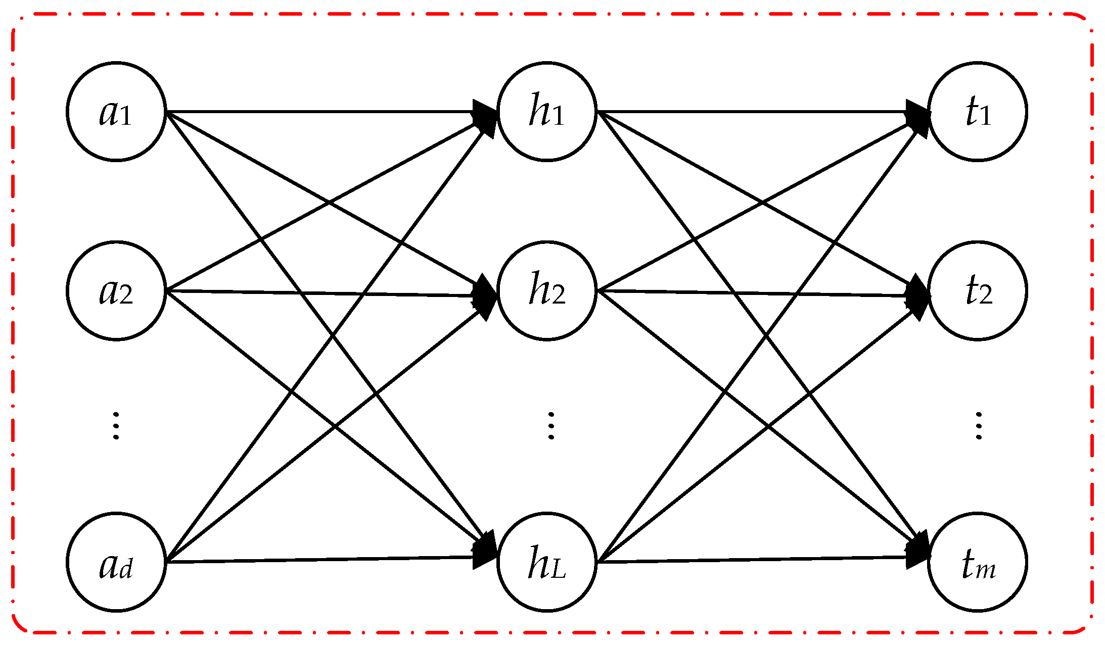
2.3. Hybrid Kernel Extreme Learning Machine

The main innovation of the extreme learning machine (ELM) [29] lies in its ability to achieve higher time efficiency while maintaining learning accuracy. Due to its exceptional pattern recognition capability, the ELM has become one of the commonly used models in fault detection.

The generalized structure of the ELM is shown in Figure 1. The input layer of the ELM, as depicted, contains d inputs, the hidden layer consists of L nodes, and the output layer has m outputs. The input weights w and biases b between the input and hidden layers are randomly generated. The expected output of the ELM network is represented as

$${\displaystyle \sum _{i=1}^L}{\beta }_{i}g(w_i·a_j+b_i)=o_j$$

(13)

where $g(·)$ represents the activation function, $w_i$ is the weight matrix, ${\beta }_i$ is the output matrix, and $b_i$ is the bias of the i-th hidden layer node.

During the network training process, it is possible to approach the training samples with zero error, i.e., ${\displaystyle \sum _{j=1}^N\left|\right|o_j-t_j\left|\right|}=0$, represented as

$$T=H\beta$$

(14)

where T is the model output, $\beta$ is the weight between the hidden layer and the output layer, and H is the output matrix of the hidden layer.

$\beta$ is represented as in ELM:

$$\beta =H^T{\left(H{H}^T+{\displaystyle \frac{I}{C}}\right)}^{-1}T$$

(15)

where T is the input sample label vector matrix, C is the penalty coefficient, and I is the identity matrix.

KELM replaces the mapping of original ELM hidden layer nodes with a kernel function, and the output is then given by

$$y=\ker (x)H^T{\left(H{H}^T+{\displaystyle \frac{I}{C}}\right)}^{-1}T$$

(16)

Selecting the radial basis function as the kernel function for KELM:

$$\ker (x_i,x_j)=\exp \left(-{\displaystyle \frac{‖x_i-x_j‖}{2{\sigma }^2}}\right)$$

(17)

where x_i is the input of the training set, x_j is the input of the test set, and $\sigma$ is the width parameter of the kernel function.

From this, the output of KELM is obtained:

$$y=\left[\begin{array}{c}\ker (x,x_1)\\ ⋮\\ \ker (x,x_n)\end{array}\right]H^T{\left(H{H}^T+{\displaystyle \frac{I}{C}}\right)}^{-1}T$$

(18)

where n is the dimension of the input vector.

Once the kernel function $\ker (x_i,x_j)$ is determined, the prediction results are generated. Hence, the choice of kernel function significantly impacts the prediction accuracy. Common kernel functions include the Poly kernel, RBF kernel, and Lin kernel, with their respective expressions given as follows:

$${\mathit{K}}_{\mathrm{Poly}}({\mathit{x}}_i,{\mathit{x}}_j)={(\mathit{x},{\mathit{x}}_i+c_1)}^b$$

(19)

$${\mathit{K}}_{\mathrm{RBF}}({\mathit{x}}_i,{\mathit{x}}_j)=\exp \left(-{\displaystyle \frac{{‖{\mathit{x}}_i-{\mathit{x}}_j‖}^2}{{\sigma }^2}}\right)$$

(20)

$${\mathit{K}}_{\mathrm{Lin}}({\mathit{x}}_i,{\mathit{x}}_j)={\mathit{x}}^T{\mathit{x}}_i$$

(21)

where c₁ and b represent the kernel parameters of the Poly kernel, while $\sigma$ denotes the kernel parameter of the RBF kernel.

A linear combination of these three kernel functions is applied to obtain a new mixed kernel function:

$${\mathit{K}}_{\mathrm{HKELM}}({\mathit{x}}_i,{\mathit{x}}_j)=c_2{\mathit{K}}_{\mathrm{Poly}}({\mathit{x}}_i,{\mathit{x}}_j)+c_3{\mathit{K}}_{\mathrm{RBF}}({\mathit{x}}_i,{\mathit{x}}_j)+c_4{\mathit{K}}_{\mathrm{Lin}}({\mathit{x}}_i,{\mathit{x}}_j)$$

(22)

where c₂, c₃, and c₄ represent the weighted coefficients of the kernel functions, with values in the range [0, 1], with the condition that

$$c_2+c_3+c_4=1$$

(23)

The hybrid function in the HKELM combines the advantages of both global and local kernels. Under different parameters, it not only demonstrates strong local search capability but also enhances its global search ability.

3. Model Design and Implementation

The proposed fault diagnosis model is primarily composed of feature extraction, feature selection, and fault pattern recognition. Initially, raw vibration data is input to the SCNN, where deep feature extraction is performed through the convolutional layers of the SCNN to capture potential fault features of rolling bearings and accurately identify key characteristics. Next, a Bernoulli-distribution-based stochastic pooling operation is employed to retain more spatial information and ensure feature diversity.

After feature extraction and selection, NGO is introduced to optimize key parameters that influence the performance of the mixed HKELM. With NGO, the hyperparameters of the HKELM are dynamically adjusted to achieve optimal classification and recognition performance.

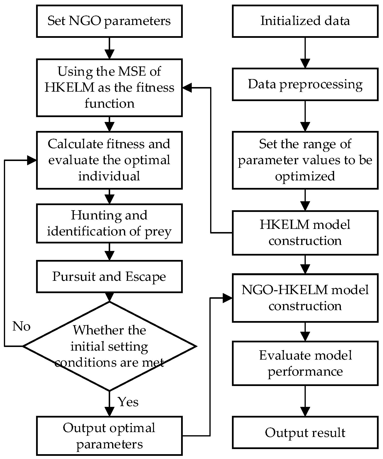
3.1. Construction of NGO–HKELM Classification Model

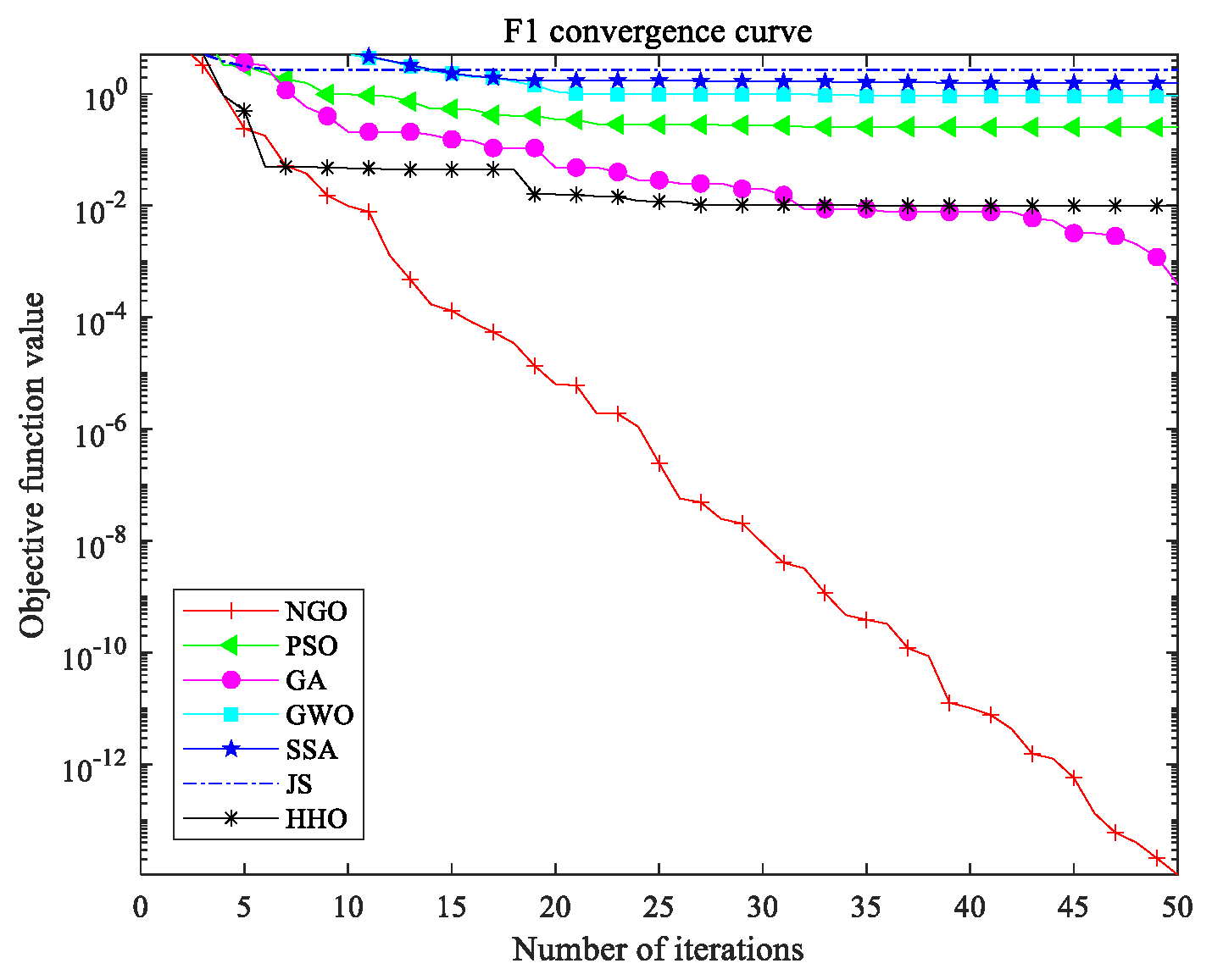
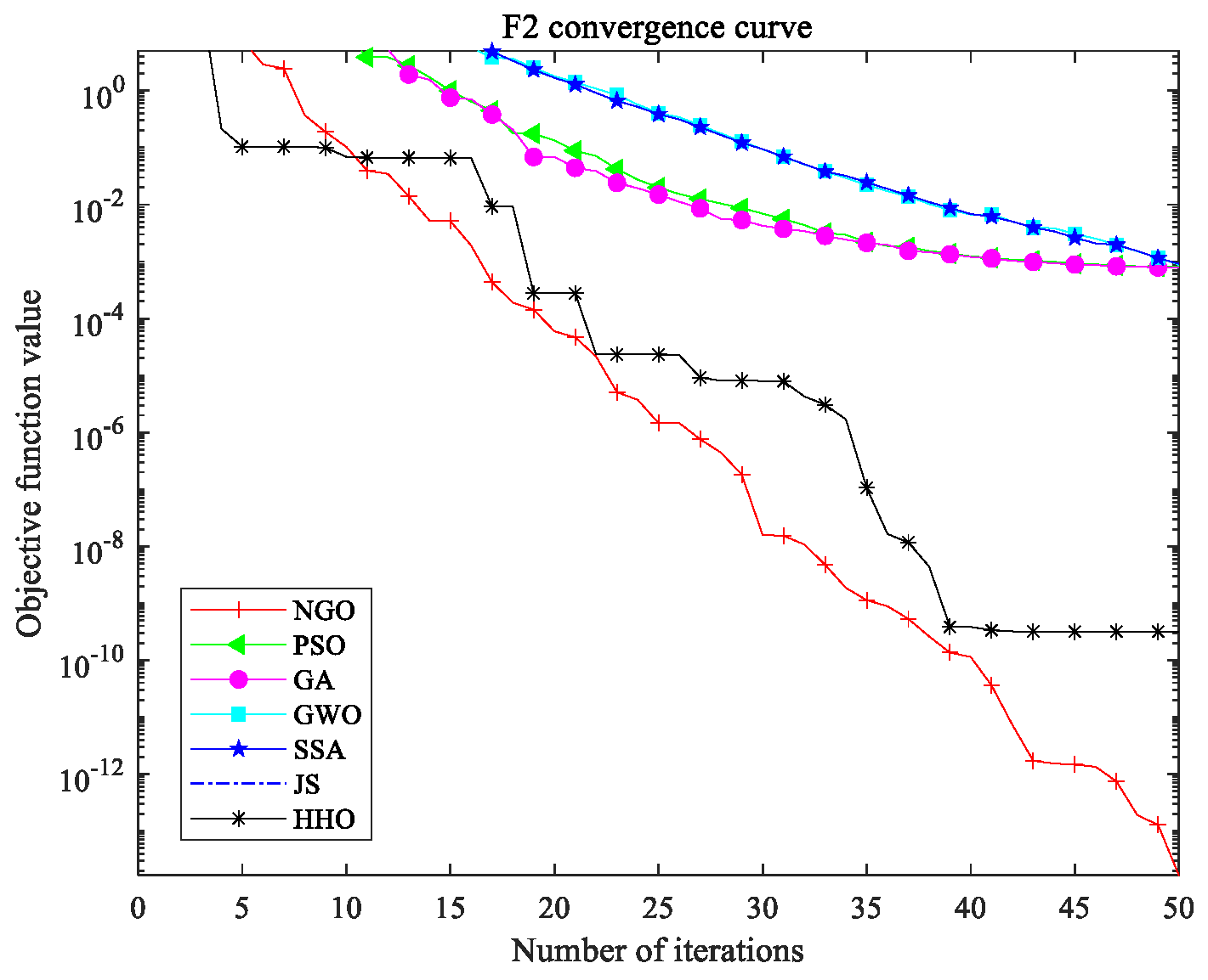
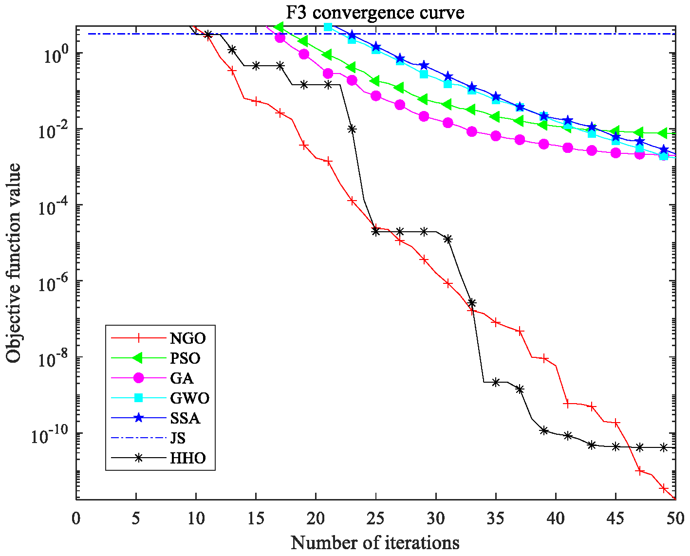
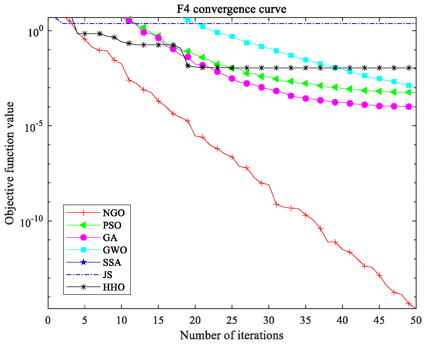
3.1.1. Discussion on the Performance of NGO Algorithm

To validate the advantages of the NGO algorithm employed in this study, the Step (F1), Sphere (F2), Rastrigin (F3), and Quartic (F4) functions (each with 30 dimensions) are selected for testing. The performance of NGO is compared with that of particle swarm optimization (PSO), genetic algorithm (GA), grey wolf optimizer (GWO), sparrow search algorithm (SSA), multi-objective jellyfish search algorithm (MOJS), and Harris hawks optimization (HHO). Specific experiments were conducted to demonstrate the rationale and effectiveness of using NGO for network parameter optimization. The parameter settings for the six selected comparison algorithms are shown in

Table 1. Six optimization algorithm parameter settings.

Algorithm	Parameter Setting	Population Number	Number of Iterations
PSO	Learning factor c1 = 1.2; c2 = 1.2; inertia weight w = 0.68	50	50
GA	Selection probability PI = 0.6; cross probability PC = 0.5	50	50
GWO	The coefficient vector component a linearly decreases from 1 to 0; the coefficient vector c is randomly taken as 0 or 1	50	50
SSA	Cross-validation fold v = 5; discoverer ratio d = 0.6	50	50
JS	$\mathrm{Distribution} \mathrm{coefficient} \alpha =0.3;$$\mathrm{coefficient} \mathrm{of} \mathrm{motion} \gamma =0.2$	50	50
HHO	Random numbers with proportional coefficients between 0 and 2	50	50

.

Figure 2, Figure 3, Figure 4 and Figure 5 show the convergence curves for the function tests conducted with seven algorithms, with the maximum number of iterations set to 50 for all algorithms. The figures clearly demonstrate that the performance of NGO exceeded those of the other algorithms across all metrics.

Table 2. Specific performance indicators of the algorithm.

Algorithm	Performance Indicator	F1	F2	F3	F4
NGO	Minimum	3.218 × 10−15	9.872 × 10−15	4.926 × 10−12	2.981 × 10−30
	Mean	0.6824	0.4976	0.9538	0.0382
	Variance	3.0157	2.3641	5.8923	0.1947
PSO	Minimum	0.014892	1.327 × 10−4	1.086 × 10−3	5.873 × 10−12
	Mean	4.9263	13.458	2.6749	0.1528
	Variance	7.8923	30.147	8.7624	0.3275
GA	Minimum	3.892 × 10−4	4.673 × 10−5	5.327 × 10−3	2.108 × 10−13
	Mean	2.3276	20.458	11.327	0.1843
	Variance	7.2159	41.327	21.458	0.7924
GWO	Minimum	1.0843	6.327 × 10−4	1.892 × 10−3	1.542 × 10−6
	Mean	2.0157	32.458	7.2159	0.0973
	Variance	7.8923	49.327	22.458	1.3276
SSA	Minimum	1.2157	8.762 × 10−4	1.327 × 10−3	9.327 × 10−7
	Mean	4.3276	44.892	20.327	0.2427
	Variance	8.4582	59.327	25.015	0.5893
JS	Minimum	1.0427	1.8923	1.2157	0.0628
	Mean	4.8923	2.3276	1.4582	0.8927
	Variance	8.3276	2.0427	0.0582	1.0427
HHO	Minimum	1.2157	8.458 × 10−4	1.892 × 10−4	9.458 × 10−7
	Mean	2.0427	26.458	8.8923	2.3276
	Variance	5.8923	30.015	23.458	2.8923

presents the specific performance indicators for the seven optimization algorithms, using minimum, mean, and variance as criteria for evaluating optimization capability. NGO achieved highly satisfactory results, significantly outperforming the other algorithms.

The proposed method was tested in a Windows 11 environment with an Intel i9-12900H CPU, an NVIDIA RTX 3060 GPU, and 16GB of RAM. The simulations were conducted using MATLAB 2024b.

As shown in

Table 3. Comparison of optimization algorithm calculation efficiency.

Algorithm	Step (F1)		Sphere (F2)		Rastrigin (F3)		Quartic (F4)
	Training (s)	Test (s)	Training (s)	Test (s)	Training (s)	Test (s)	Training (s)	Test (s)
NGO	0.85	0.0011	0.87	0.001	0.82	0.0012	0.79	0.0013
PSO	1.23	0.0015	1.25	0.0019	1.22	0.0014	1.31	0.0017
GA	3.51	0.0023	3.61	0.0033	3.55	0.0039	3.58	0.0034
GWO	1.05	0.0018	1.12	0.0017	1.07	0.0018	1.04	0.0013
SSA	1.12	0.0019	1.15	0.0018	1.18	0.0015	1.21	0.0015
JS	2.86	0.0024	2.93	0.0022	2.87	0.0027	2.83	0.0026
HHO	1.15	0.0018	1.24	0.0013	1.23	0.0013	1.19	0.0012

, the NGO algorithm significantly outperformed other algorithms in terms of computational efficiency. It exhibited the shortest training times across all test functions (F1–F4) and maintained a stable testing time of 0.001 s, demonstrating excellent convergence speed and real-time performance. Algorithms such as PSO, GWO, SSA, and HHO showed moderate performance, while the GA and JS algorithms had relatively lower computational efficiency, likely due to the increased complexity introduced by their global search mechanisms. Based on this comprehensive comparison, the NGO algorithm was selected for optimization in this study.

3.1.2. Optimizing HKELM Using NGO

HKELM significantly enhances its data-fitting capability by incorporating multiple kernel functions. However, the introduction of multiple kernels inevitably increases the number of parameters, and the values of these critical parameters can significantly impact model performance. Therefore, this study employed NGO to optimize five key parameters c₁, c₃, σ, d, and C within HKELM.

The construction process of the NGO–HKELM model is as shown in Figure 6.

(1)

The population size of the northern sparrowhawk, fitness function, number of iterations, and other parameters are set, and the initial positions of the sparrowhawk individuals are generated.

(2)

The value ranges for the parameters to be optimized in the HKELM network are set, and the HKELM model is constructed. The mean squared error (MSE) of the HKELM is used as the fitness function for NGO.

(3)

The fitness values are calculated, and the optimal northern sparrowhawk individual at the current moment is evaluated.

(4)

The sparrowhawk state is updated according to Equations (1)–(6), continuing the process of prey search and recognition, pursuit, and escape.

(5)

It is determined whether the initial set conditions are met. If so, the current optimal three-dimensional values corresponding to the northern sparrowhawk individual are output; otherwise, step (3) is repeated to continue the optimization process.

(6)

The optimal parameters are obtained, and the NGO–HKELM model is constructed. The model’s performance is evaluated, and the prediction results are output.

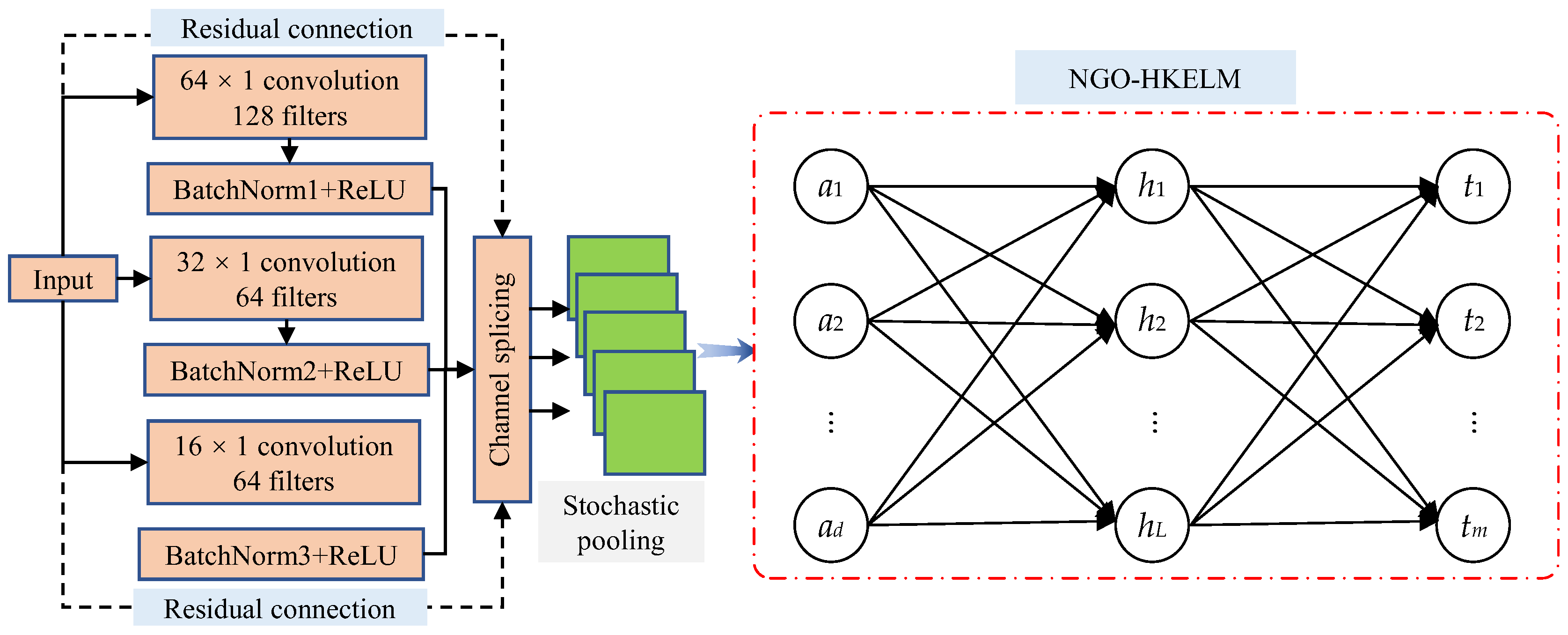
3.2. SCNN and NGO–HKELM Model Network Structure

This research focuses on rolling bearings, with vibration signals represented as one-dimensional data. To accommodate the input characteristics of these one-dimensional vibration signals, the convolutional and pooling layers of the constructed model are designed with one-dimensional structures. Compared to traditional CNNs, the following improvements are made:

(1)

This study innovatively designs a multi-scale feature extraction architecture that overcomes the limitations of traditional CNNs, which typically rely on a single convolution kernel size. The architecture includes three parallel feature extraction pathways: the first pathway employs a large 64 × 1 convolution kernel to focus on extracting low-frequency features that reflect the long-term operational state of the equipment; the second pathway utilizes a medium-sized 32 × 1 convolution kernel to capture transitional features at intermediate time scales; the third pathway uses a compact 16 × 1 convolution kernel specifically for detecting transient impact signals. The outputs of these pathways are fused by concatenating along the channel dimension, followed by a 1 × 1 convolution for feature compression and dimensionality reduction. This multi-scale collaborative processing mechanism significantly enhances the model’s ability to perceive fault features across different frequency bands.

(2)

A residual learning mechanism is incorporated into the deep neural network architecture, effectively addressing the gradient vanishing problem in deep networks by constructing cross-layer connection pathways. This design not only ensures the effective flow of gradients during the backpropagation process but also substantially improves the model’s feature representation capability.

(3)

A Bernoulli-distribution-based random pooling operation is proposed, which better captures underlying changes in the data and preserves the spatial structure information of feature maps as much as possible.

Figure 7 illustrates the SCNN–NGO–HKELM hybrid network architecture proposed in this study. The model adopts an end-to-end design, enabling direct processing of raw vibration signal inputs. A hierarchical feature extraction strategy is employed, wherein alternating convolution operations and nonlinear pooling progressively build multi-level fault feature representations. Notably, a cross-layer connection mechanism is introduced in the deeper layers of the network, effectively enhancing gradient propagation efficiency. In terms of network optimization, batch normalization units are integrated after each convolution operation, significantly improving the model’s training stability.

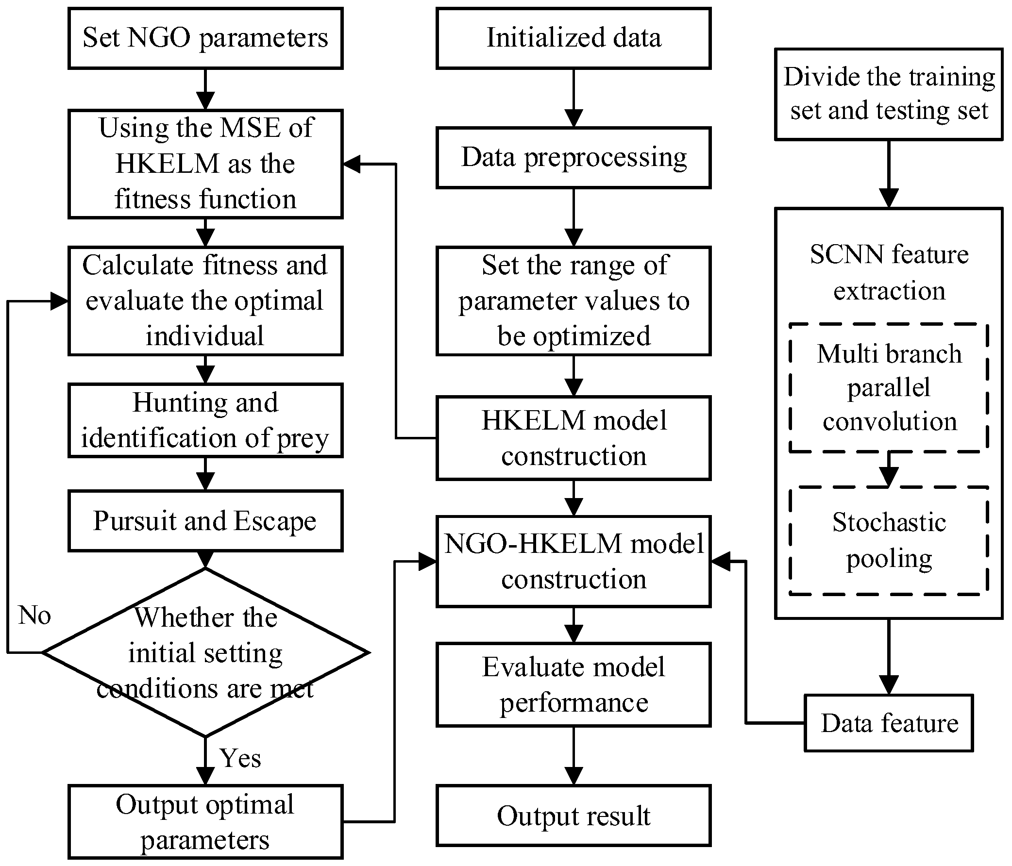
3.3. Model Flowchart and Algorithm Steps

The fault diagnosis process based on SCNN and NGO–HKLEM is illustrated in Figure 8 and can be divided into five steps:

(1)

The SCNN model is constructed, utilizing the multi-branch parallel convolution and Bernoulli-distribution-based random pooling layers within the SCNN framework for feature extraction.

(2)

The initialization weights, thresholds, and other parameters of the HKELM network are determined, along with the range of values for the parameters to be optimized.

(3)

The population is initialized, and the training error of the HKELM is used as the fitness value.

(4)

The fitness of the hawk population is evaluated, and the hawk positions are updated based on the predatory behavior, search, pursuit, and evasion patterns of the northern goshawk.

(5)

A check is performed to determine if the parameter optimization condition is satisfied. If the condition is met, the optimal hyperparameters are assigned to the HKELM, and the NGO–HKELM model is constructed. If the condition is not met, step (3) is repeated.

(6)

The fault state is identified using the constructed NGO–HKELM model, and the diagnostic results are output.

Figure 8. Fault diagnosis process based on SCNN and NGO–HKELM.

Figure 8. Fault diagnosis process based on SCNN and NGO–HKELM.

4. Case Introduction

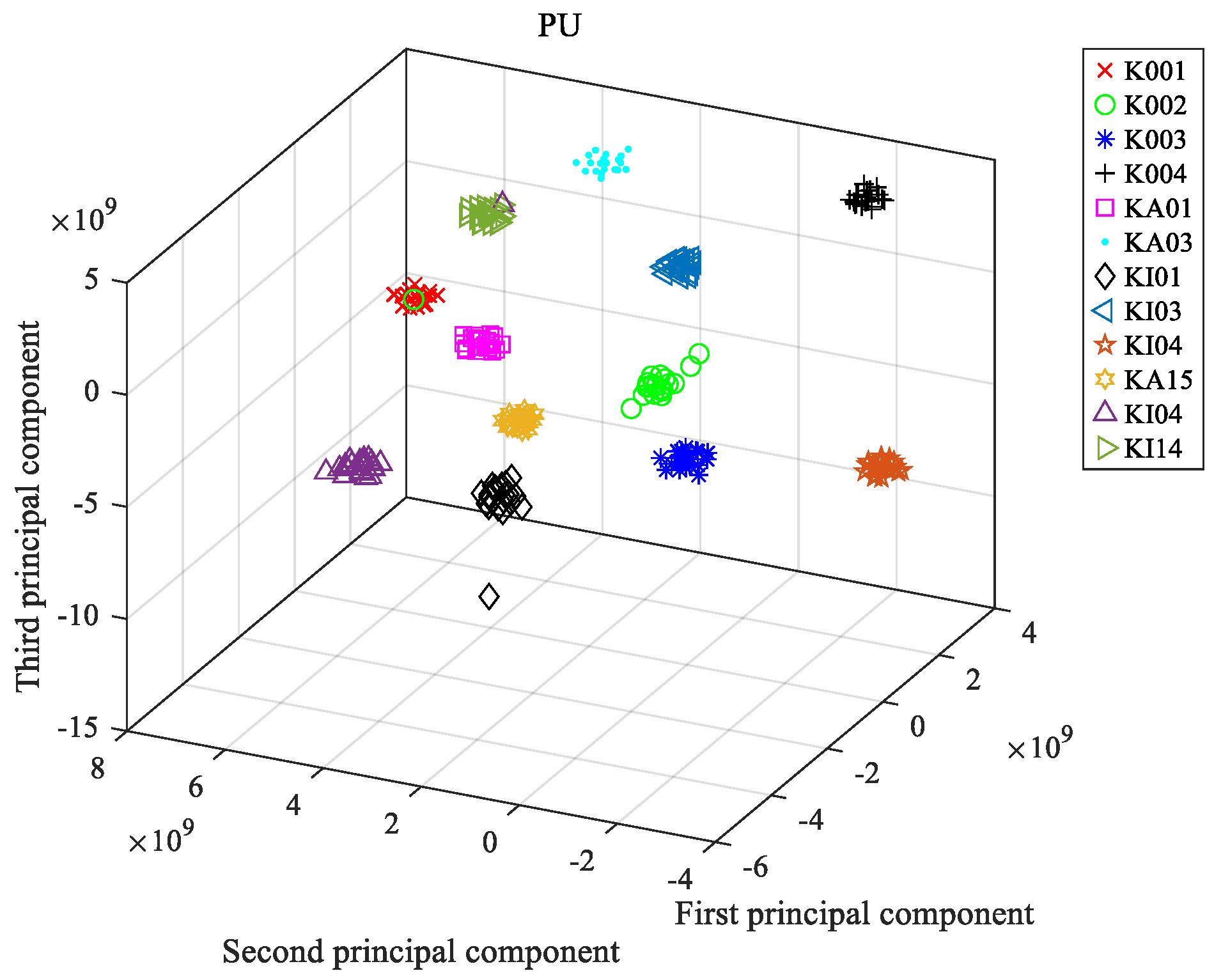
4.1. Data Description

The bearing dataset provided by Paderborn University, Germany [31], was categorized into three main groups. The first group consisted of data collected from six healthy bearing units. The second group included data from twelve bearings with induced damage, where the damage was caused by three different methods: electrical discharge machining, drilling-induced damage, and manual electric engraving damage. The third group comprised data from fourteen accelerated life tests, which were conducted using a scientific test rig to obtain failure data from bearings subjected to actual damage.

To ensure the selected data for the simulation experiments was more representative, as shown in

Table 4. Fault types of rolling bearings in dataset from the Paderborn University.

Label	Fault Type	Fault Location	Cause of Fault	Sample Size
1	K001	Fault-free	Healthy	100
2	K002	Fault-free	Healthy	100
3	K003	Fault-free	Healthy	100
4	K004	Fault-free	Healthy	100
5	KA01	Outer race	Electrical discharge machining	100
6	KA03	Outer race	Electrical discharge machining	100
7	KI01	Inner race	Manual electric engraving damage	100
8	KI03	Inner race	Manual electric engraving damage	100
9	KA04	Outer race	Accelerated life test	100
10	KA15	Outer race	Accelerated life test	100
11	KI04	Inner race	Accelerated life test	100
12	KI14	Inner race	Accelerated life test	100

, four fault states were chosen from each of the three major data categories for analysis. This resulted in a study of 12 different fault types, with each fault type consisting of 100 samples, totaling 1200 samples. From each fault type, 80 samples were randomly selected as the training set, and the remaining 20 samples were used as the testing set. Thus, the total number of training samples was 960, and the total number of testing samples was 240.

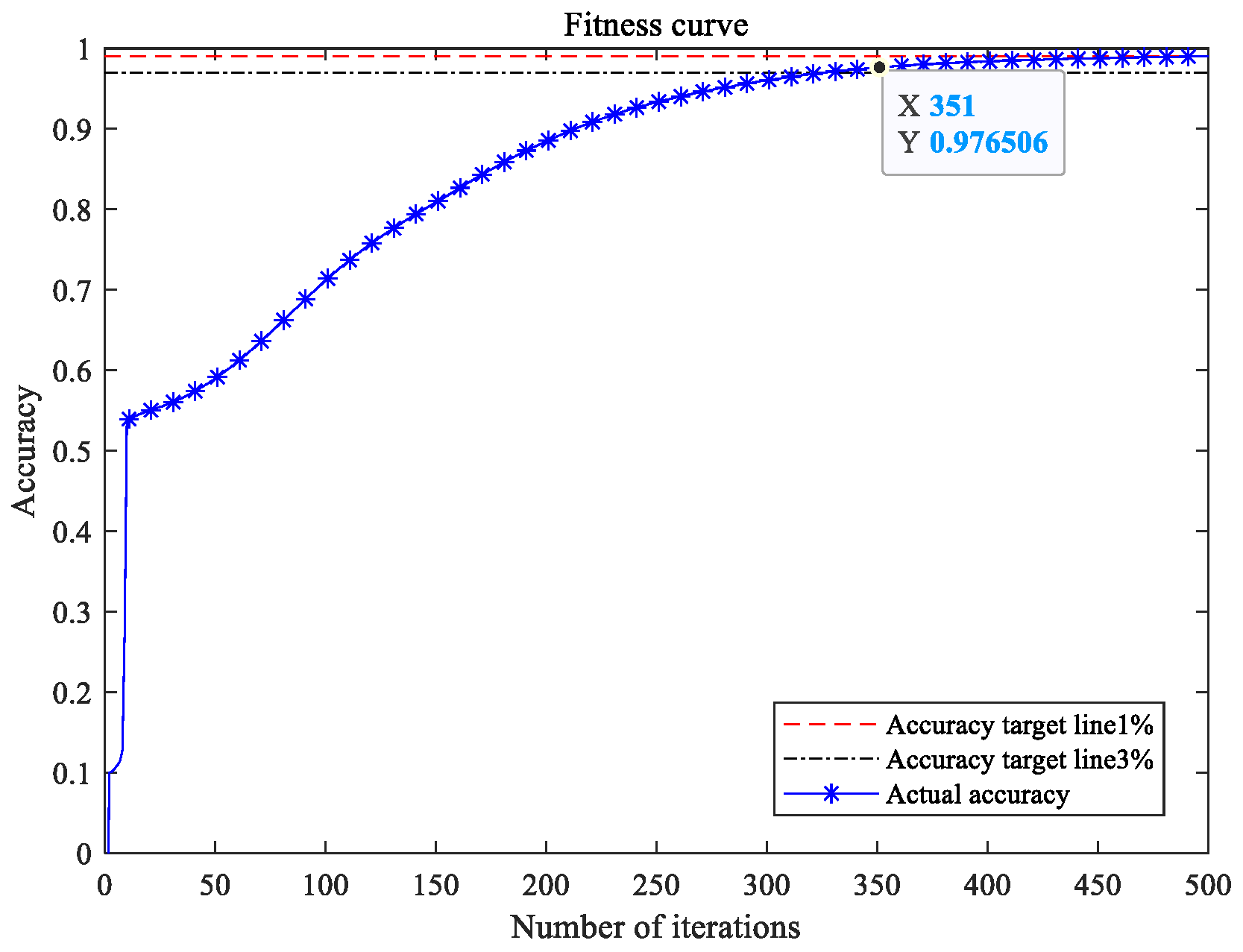
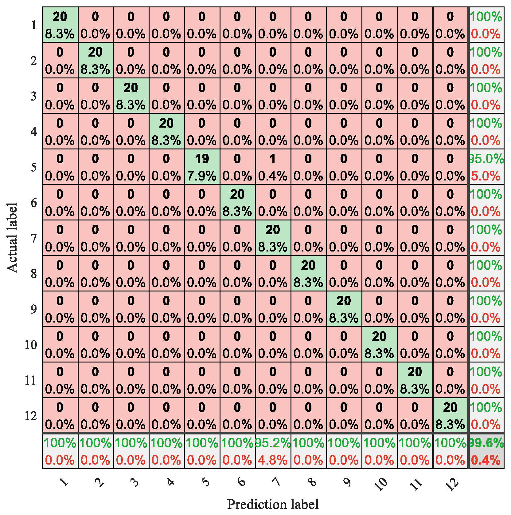
4.2. Experimental Plan and Analysis

Figure 9 illustrates the performance evolution curve of the proposed model trained on the PU dataset. The experimental results indicate that the model demonstrates excellent convergence characteristics: during the early stages of training (after 351 iterations), the classification accuracy rapidly increased to below 97%. As the optimization process progressed, the model performance stabilized around iteration 460, with the final classification accuracy exceeding 99%. To ensure full convergence, the maximum number of iterations was set to 500. The curve revealed that the fitness value eventually stabilized at an optimal level, which validated the effectiveness and reliability of the proposed fault diagnosis model.

Figure 10 presents the confusion matrix for the test set, showing the diagnostic accuracy for each of the 12 fault types. It also includes the overall fault diagnosis accuracy for the test set. The proposed model achieved a 100% diagnostic accuracy for fault types K001, K002, K003, K004, KA03, KI01, KI03, KA04, KA15, KI04, and KI14. For fault type KA01, the accuracy was 95%, with one sample incorrectly classified as fault type KI01. The overall fault diagnosis accuracy for the test set reached 99.6%, which demonstrated that the proposed model effectively solved the fault diagnosis problem for rolling bearings.

To better visualize the feature extraction performance of the proposed model, the feature data from the test set was visualized using t-distributed stochastic neighbor embedding (t-SNE). Figure 11 shows a scatter plot of the PU test set’s feature extraction. The clustering effect of the fault states is clearly visible, with minimal misclassification. Each fault state is well-separated, indicating the model’s high performance in distinguishing between fault types.

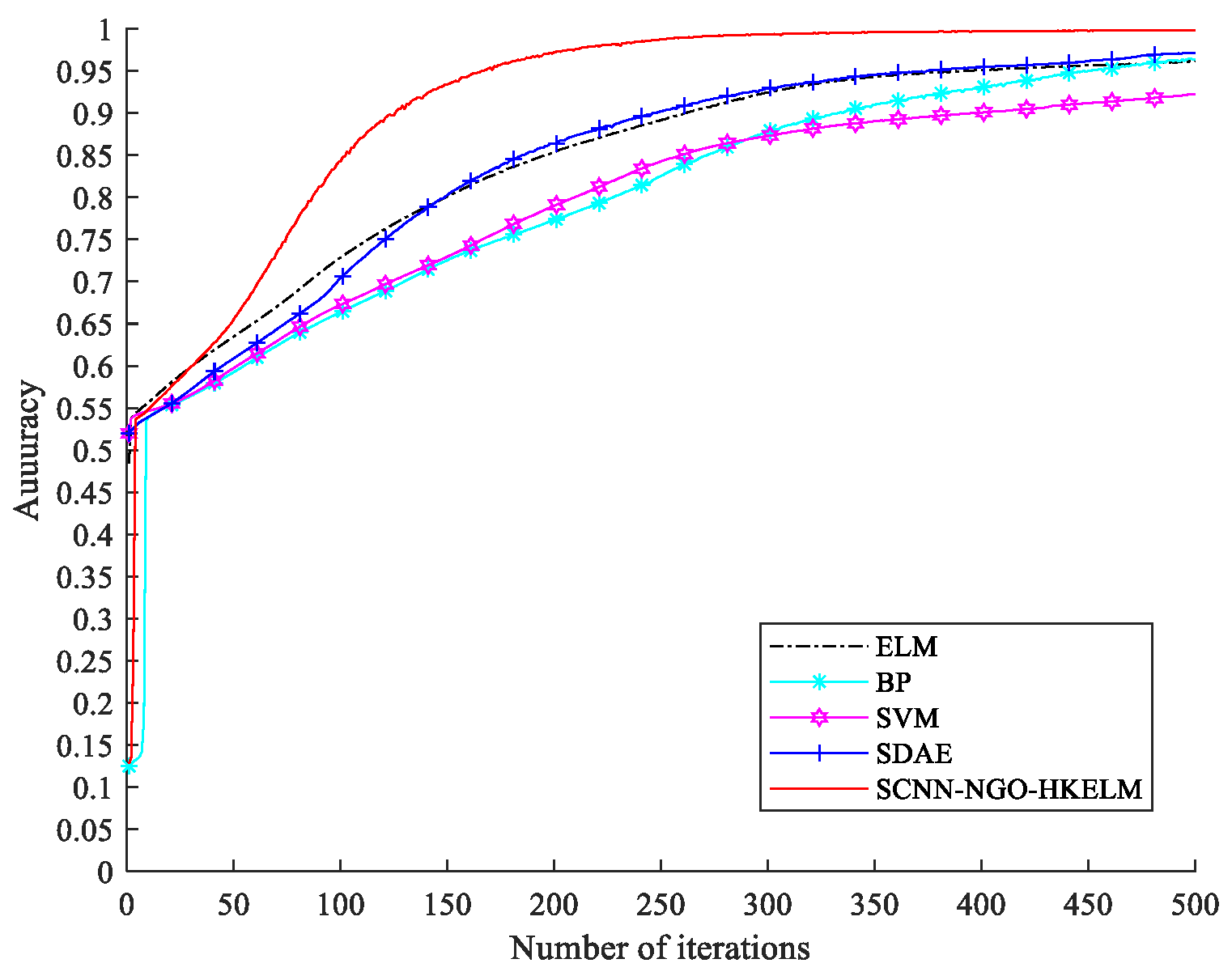
4.3. Comparative Experiment

To evaluate the performance advantages of the proposed algorithm, a comprehensive comparative experimental setup was designed, selecting four representative machine learning models as baseline methods, including both shallow and deep learning models. The parameters for each comparison algorithm were rigorously tuned, with the specific settings as follows:

(1)

SVM: The regularization parameter was set to 1, and the Gaussian kernel width was 0.1.

(2)

BP: The network topology consisted of a 41–26–32 three-hidden-layer structure, with an initial learning rate of 0.02.

(3)

ELM: The regularization coefficient was set to 1, the kernel function parameter was 0.15, and the number of hidden layer nodes was determined through cross-validation.

(4)

Stacked denoising autoencoder (SDAE): A layer-wise greedy training strategy was employed, with a learning rate of 1, input noise ratio of 0.1, and a batch size of 200 for training samples.

Figure 12 presents a comparison of the accuracy curves for various network test sets. For both SVM and BP networks, the fault diagnosis accuracy was significantly lower than that of NGO–HKELM. Although ELM and SDAE demonstrated better diagnostic performance than SVM and BP, their accuracy was still far inferior to that of NGO–HKELM.

As shown in

Table 5. Comparison of computational efficiency among different networks.

Network	ELM	BP	SVM	SDAE	SCNN	SCNN–NGO–HKELM
Training time (s)	5.86	7.52	12.37	25.77	13.62	15.63
Test time (s)	247	2.53	3.98	6.96	3.35	4.56

, a comparative analysis of the training and testing times for different networks was conducted. Due to its shallow model structure, the best performance was achieved in terms of both training and testing efficiency. SCNN–NGO–HKELM exhibited slightly lower testing efficiency compared to the two deep learning models, SDAE and SCNN. This was primarily due to a trade-off between accuracy improvement and computational efficiency. However, its testing time of 4.56 s was fully sufficient to meet the real-time requirements for fault diagnosis in complex industrial settings.

The computational complexity of SCNN–NGO–HKELM primarily stems from the convolution kernel optimization in NGO ($O(I\times P\times K\times H_{in}\times W_{in})$) and the kernel matrix construction in HKELM ($O(N^{2}d)$). While it exceeds that of the basic SCNN, its training complexity remains significantly lower than those of traditional deep learning models due to the elimination of CNN backpropagation. The additional decision overhead introduced by HKELM during the testing phase ($O(N_{sv}\times d)$) exhibited linear scalability and was much smaller than the number of training samples, ensuring real-time performance in industrial applications. This design sacrifices a controllable computational cost in exchange for high accuracy and robustness, aligning with the core requirement in industrial fault diagnosis: prioritizing reliability over microsecond-level latency.

5. Conclusions

This study addresses the technical challenges of feature extraction and diagnostic accuracy in rolling bearing fault detection within industrial scenarios. An innovative intelligent diagnostic system is proposed, integrating a stochastic convolutional neural network with an optimized hybrid kernel extreme learning machine.

(1)

An improved SCNN architecture with multi-scale perception capability is developed. This architecture captures cross-frequency features through parallel multi-branch convolution paths, combined with a probabilistic sampling-based random pooling layer, significantly enhancing the discriminative power of fault features.

(2)

The modified NGO algorithm is introduced to adaptively adjust the parameters of the HKELM.

(3)

Comparative experiments based on the Paderborn University standard bearing dataset (12 fault types, 4 load conditions) demonstrated that the proposed method significantly outperformed traditional intelligent algorithms in diagnostic accuracy.

However, the proposed model still has limitations in terms of performance for complex industrial environments. Future work will focus on developing intelligent fault diagnosis models that are applicable across multiple operating conditions, providing new technological support for the field of fault diagnosis.

References

1. Qian, Q.; Zhang, B.; Li, C.; Mao, Y.; Qin, Y. Federated transfer learning for machinery fault diagnosis: A comprehensive review of technique and application. Mech. Syst. Signal Process. 2025, 223, 111837. [Google Scholar] [CrossRef]
2. Xiao, Y.; Shao, H.; Yan, S.; Wang, J.; Peng, Y.; Liu, B. Domain generalization for rotating machinery fault diagnosis: A survey. Adv. Eng. Inform. 2025, 64, 103063. [Google Scholar] [CrossRef]
3. Xu, Y.; Ge, X.; Guo, R.; Shen, W. Recent advances in model-based fault diagnosis for lithium-ion batteries: A comprehensive review. Renew. Sustain. Energy Rev. 2025, 207, 114922. [Google Scholar] [CrossRef]
4. Wang, L.; Zhao, W. An ensemble deep learning network based on 2D convolutional neural network and 1D LSTM with self-attention for bearing fault diagnosis. Appl. Soft Comput. 2025, 172, 112889. [Google Scholar] [CrossRef]
5. Ren, X.; Wang, S.; Zhao, W.; Kong, X.; Fan, M.; Shao, H.; Zhao, K. Universal federated domain adaptation for gearbox fault diagnosis: A robust framework for credible pseudo-label generation. Adv. Eng. Inform. 2025, 65, 103233. [Google Scholar] [CrossRef]
6. Tian, J.; Jiang, Y.; Zhang, J.; Luo, H.; Yin, S. A novel data augmentation approach to fault diagnosis with class-imbalance problem. Reliab. Eng. Syst. Saf. 2024, 243, 109832. [Google Scholar] [CrossRef]
7. Yang, B.; Lei, Y.; Li, X.; Li, N. Targeted transfer learning through distribution barycenter medium for intelligent fault diagnosis of machines with data decentralization. Expert Syst. Appl. 2024, 244, 122997. [Google Scholar] [CrossRef]
8. Yu, Y.; Karimi, H.R.; Gelman, L.; Liu, X. A novel digital twin-enabled three-stage feature imputation framework for non-contact intelligent fault diagnosis. Adv. Eng. Inform. 2025, 66, 103434. [Google Scholar] [CrossRef]
9. Ardali, N.R.; Zarghami, R.; Gharebagh, R.S.; Mostoufi, N. A data-driven fault detection and diagnosis by NSGAII-t-SNE and clustering methods in the chemical process industry. Comput. Aided Chem. Eng. 2022, 49, 1447–1452. [Google Scholar]
10. Tarcsay, B.L.; Bárkányi, Á.; Chován, T.; Németh, S. A Dynamic Principal Component Analysis and Fréchet-Distance-Based Algorithm for Fault Detection and Isolation in Industrial Processes. Processes 2022, 10, 2409. [Google Scholar] [CrossRef]
11. Meng, L.; Su, Y.; Kong, X.; Xu, T.; Lan, X.; Li, Y. Intelligent fault diagnosis of gearbox based on differential continuous wavelet transform-parallel multi-block fusion residual network. Measurement 2023, 206, 112318. [Google Scholar] [CrossRef]
12. Wang, X.; Shi, J.; Zhang, J. A power information guided-variational mode decomposition (PIVMD) and its application to fault diagnosis of rolling bearing. Digit. Signal Process. 2022, 132, 103814. [Google Scholar] [CrossRef]
13. Jalayer, M.; Orsenigo, C.; Vercellis, C. Fault detection and diagnosis for rotating machinery: A model based on convolutional LSTM, Fast Fourier and continuous wavelet transforms. Comput. Ind. 2021, 125, 103378. [Google Scholar] [CrossRef]
14. Da Silva, P.R.N.; Gabbar, H.A.; Junior, P.V.; Junior, C.T.d.C. A new methodology for multiple incipient fault diagnosis in transmission lines using QTA and Naïve Bayes classifier. Int. J. Electr. Power Energy Syst. 2018, 103, 326–346. [Google Scholar] [CrossRef]
15. Prasojo, R.A.; Putra, M.A.A.; Apriyani, M.E.; Apriyani, M.E.; Rahmanto, A.N.; Ghoneim, S.S.; Mahmoud, K.; Lehtonen, M.; Darwish, M.M. Precise transformer fault diagnosis via random forest model enhanced by synthetic minority over-sampling technique. Electr. Power Syst. Res. 2023, 220, 109361. [Google Scholar] [CrossRef]
16. Cao, H.; Sun, P.; Zhao, L. PCA-SVM method with sliding window for online fault diagnosis of a small pressurized water reactor. Ann. Nucl. Energy 2022, 171, 109036. [Google Scholar] [CrossRef]
17. Chen, X.; Qi, X.; Wang, Z.; Cui, C.; Wu, B.; Yang, Y. Fault diagnosis of rolling bearing using marine predators algorithm-based support vector machine and topology learning and out-of-sample embedding. Measurement 2021, 176, 109116. [Google Scholar] [CrossRef]
18. Kumar, R.S.; Raj, I.G.C.; Alhamrouni, I.; Saravanan, S.; Prabaharan, N.; Ishwarya, S.; Gokdag, M.; Salem, M. A combined HT and ANN based early broken bar fault diagnosis approach for IFOC fed induction motor drive. Alex. Eng. J. 2023, 66, 15–30. [Google Scholar] [CrossRef]
19. Wang, H.; Zheng, J.; Xiang, J. Online bearing fault diagnosis using numerical simulation models and machine learning classifications. Reliab. Eng. Syst. Saf. 2023, 234, 109142. [Google Scholar] [CrossRef]
20. Hakim, M.; Omran, A.A.B.; Ahmed, A.N.; Al-Waily, M.; Abdellatif, A. A systematic review of rolling bearing fault diagnoses based on deep learning and transfer learning: Taxonomy, overview, application, open challenges, weaknesses and recommendations. Ain Shams Eng. J. 2022, 14, 101945. [Google Scholar] [CrossRef]
21. Gao, S.; Xu, L.; Zhang, Y.; Pei, Z. Rolling bearing fault diagnosis based on SSA optimized self-adaptive DBN. ISA Trans. 2022, 128, 485–502. [Google Scholar] [CrossRef] [PubMed]
22. Niu, G.; Wang, X.; Golda, M.; Mastro, S.; Zhang, B. An optimized adaptive PReLU-DBN for rolling element bearing fault diagnosis. Neurocomputing 2021, 445, 26–34. [Google Scholar] [CrossRef]
23. Gao, D.; Zhu, Y.; Ren, Z.; Yan, K.; Kang, W. A novel weak fault diagnosis method for rolling bearings based on LSTM considering quasi-periodicity. Knowl.-Based Syst. 2021, 231, 107413. [Google Scholar] [CrossRef]
24. Zhao, K.; Jia, F.; Shao, H. A novel conditional weighting transfer Wasserstein auto-encoder for rolling bearing fault diagnosis with multi-source domains. Knowl.-Based Syst. 2023, 262, 110203. [Google Scholar] [CrossRef]
25. Xiang, Z.; Zhang, X.; Zhang, W.; Xia, X. Fault diagnosis of rolling bearing under fluctuating speed and variable load based on TCO spectrum and stacking auto-encoder. Measurement 2019, 138, 162–174. [Google Scholar] [CrossRef]
26. Qu, J.; Yu, L.; Yuan, T.; Tian, Y. Adaptive fault diagnosis algorithm for rolling bearings based on one-dimensional convolutional neural network. Chin. J. Sci. Instrum. 2018, 39, 134–143. [Google Scholar]
27. Huo, C.; Jiang, Q.; Shen, Y.; Qian, C.; Zhang, Q. New transfer learning fault diagnosis method of rolling bearing based on ADC-CNN and LATL under variable conditions. Measurement 2022, 188, 110587. [Google Scholar] [CrossRef]
28. Li, K.; Xiong, M.; Li, F.; Su, L.; Wu, J. A novel fault diagnosis algorithm for rotating machinery based on a sparsity and neighborhood preserving deep extreme learning machine. Neurocomputing 2019, 350, 261–270. [Google Scholar] [CrossRef]
29. He, C.; Wu, T.; Gu, R.; Jin, Z.; Ma, R.; Qu, H. Rolling bearing fault diagnosis based on composite multiscale permutation entropy and reverse cognitive fruit fly optimization algorithm–extreme learning machine. Measurement 2021, 173, 108636. [Google Scholar] [CrossRef]
30. Gong, J.; Yang, X.; Wang, H.; Shen, J.; Liu, W.; Zhou, F. Coordinated method fusing improved bubble entropy and artificial Gorilla Troops Optimizer optimized KELM for rolling bearing fault diagnosis. Appl. Acoust. 2022, 195, 108844. [Google Scholar] [CrossRef]
31. Lessmeier, C.; Kimotho, J.K.; Zimmer, D.; Sextro, W. Condition monitoring of bearing damage in electromechanical drive systems by using motor current signals of electric motors: A benchmark data set for data-driven classification. In Proceedings of the PHM Society European Conference, Bilbao, Spain, 5–8 July 2016. [Google Scholar]
Figure 1. Generalized structure diagram of ELM.
Mathematics 13 02004 g001
Figure 2. Step function (F1) test results.
Mathematics 13 02004 g002
Figure 3. Sphere function (F2) test results.
Mathematics 13 02004 g003
Figure 4. Rastrigin function (F3) test results.
Mathematics 13 02004 g004
Figure 5. Quartic function (F4) test results.
Mathematics 13 02004 g005
Figure 6. NGO–HKELM fault diagnosis flow chart.
Mathematics 13 02004 g006
Figure 7. SCNN and NGO–HKELM network architecture.
Mathematics 13 02004 g007
Figure 9. Fitness curve of training set.
Mathematics 13 02004 g009
Figure 10. Test set confusion matrix.
Mathematics 13 02004 g010
Figure 11. Scatter diagram.
Mathematics 13 02004 g011
Figure 12. Accuracy curves for various network.
Mathematics 13 02004 g012