Distributed Control Strategy for Automatic Power Sharing of Hybrid Energy Storage Systems with Constant Power Loads in DC Microgrids

Abstract

Hybrid energy storage systems (HESSs), with superior transient response characteristics compared to conventional battery (BAT) systems, have emerged as an effective solution for power balance. However, the high penetration of constant power loads (CPLs) introduces destabilization risks to the system. To address this challenge, this paper proposes a novel hierarchical control strategy to achieve voltage stabilization and accurate current sharing. First, this paper proposes an improved P–V² controller as the primary controller. It utilizes virtual conductance to replace the fixed coefficients of traditional droop controllers to achieve automatic power allocation between supercapacitors (SCs) and BATs, while eliminating the effects of CPLs on the voltage–current relationship. Second, based on traditional distributed control, the secondary control layer integrates a dynamic event-triggered communication mechanism, which reduces communication bandwidth requirements while maintaining precise current sharing across distributed buses. Finally, simulation and experimental results validate the effectiveness and robustness of the proposed control strategy.

1. Introduction

In recent years, renewable energy sources (RES) have experienced significant development. However, their power fluctuation characteristics pose challenges to grid stability [1,2]. Thus, hybrid energy storage systems (HESS) in DC microgrids have been extensively studied due to their fast response capability [3] and absence of reactive power control requirements [4]. However, with the advancement of power systems, CPLs have proliferated, which pose challenges to stable system operation. Therefore, this paper primarily investigates voltage stability and current sharing in hybrid energy storage systems within multi-bus DC microgrids, with particular consideration given to the nonlinear voltage–current relationships caused by CPLs.

In multi-bus hybrid energy storage systems, droop control is typically employed in local controllers to stabilize bus voltage and manage power sharing between SCs and BATs on the local bus [5]. However, conventional droop control cannot automatically assign transient power to SCs and steady-state power to BATs, thereby failing to fully utilize the transient advantages of hybrid energy storage systems. To address this issue, numerous control methods have been proposed. The standard frequency-domain decomposition approach utilizes digital signal processing techniques techniques, applying high/low-pass filters to split power demands into separate spectral bands. This framework assigned fast-varying power (high-frequency) to SCs and slow-varying components (low-frequency) to BATs [6,7,8]. Optimization-based strategies, as in [9,10], employed advanced control architectures. Ref. [9] introduced a HESS design with BATs linked via bidirectional converters and SCs directly coupled to the DC bus, integrating PI regulators and fuzzy logic to stabilize voltage and mitigate battery current transients. Ref. [10] extended this by developing a multi-mode fuzzy controller for solar–HESS integration. Although these centralized methods can achieve theoretical power management efficacy, real-world deployment encounters critical limitations. Communication delays between central and local controllers degrade dynamic responsiveness, while single-point failure risks in centralized systems threaten microgrid robustness [11]. Then, Ref. [12] proposed a decentralized improved I–V droop control strategy by replacing the constant droop coefficient in the I–V droop control with virtual impedance. Due to the influence of line impedance, Ref. [13] proposed an improved P–V² control strategy to eliminate its effects. However, none of the aforementioned control strategies account for the impact of CPLs on the system.

As the name implies, CPLs inherently exhibit negative impedance characteristics in DC microgrid systems due to their constant power consumption. This negative impedance behavior, when interacting with other power electronic components, reduces system damping and may even induce instability [14]. Consequently, the adverse effects of CPLs must be taken into account when designing control strategies for HESS. Currently, passive damping methods have been extensively investigated [15,16]. However, the integration of additional physical components increases system losses and economic costs for power grids. Moreover, these methods often become ineffective under real-world physical constraints. To address this issue, researchers have proposed active damping approaches [17,18]. In [17], virtual impedance was introduced, but this deteriorates load performance. Ref. [18] proposed a robust stabilization strategy utilizing virtual resistance. While this method achieved simplified system stabilization, it introduced undesirable DC bus voltage fluctuations. Therefore, this paper proposes an improved P–V² strategy for primary control, which replaces fixed coefficients in conventional control with virtual conductance to enable autonomous power allocation between BATs and SCs on each bus, while simultaneously decoupling the nonlinear voltage–current relationships induced by CPLs.

With the expansion of the power grid scale, multi-bus microgrids have garnered significant research attention compared to single-bus microgrid systems [19]. For multi-bus DC microgrids, while traditional droop control can achieve bus voltage stabilization, precise current sharing among different buses requires secondary control for regulation [20]. Ref. [21] proposed a dual-module secondary controller strategy based on the consensus algorithm, enabling simultaneous voltage stabilization and power sharing regulation. Ref. [22] developed a control scheme employing a discrete consensus algorithm in an islanded photovoltaic-storage DC microgrid model. Ref. [23] designed a hybrid distributed secondary controller comprising continuous and discrete components. Ref. [24] introduced a consensus control strategy using the leader–follower approach, which reduced communication links between follower nodes and the bus, thereby alleviating communication overhead while maintaining microgrid control performance. However, these studies focus on control strategies under free communication conditions. Ref. [25] incorporated a dynamic event-triggered communication mechanism into the secondary control layer to reduce the communication burden. Inspired by this, our work integrated dynamic event-triggered communication into the secondary control framework to reduce communication pressure and prevent control strategy failure caused by limited system communication bandwidth.

In summary, to achieve (1) automatic power allocation between BATs and SCs, (2) current sharing among multiple buses with reduced communication burden, and (3) elimination of the adverse effects caused by CPLs, this paper proposes a distributed control strategy enabling autonomous power distribution and multi-bus current equalization. The key innovations are as follows:

• The primary control layer implements an enhanced P–V² droop control mechanism utilizing adaptive virtual impedance instead of fixed droop coefficients. This strategic modification permits SCs to dynamically compensate for transient power fluctuations while BATs maintain steady-state power supply, collectively optimizing the system’s transient performance. Furthermore, this control scheme effectively eliminates the adverse impacts induced by CPLs;
• A secondary control method is proposed that achieves current sharing among multiple buses while maintaining voltage stabilization, thereby preventing excessive consumption in any individual unit and prolonging the system’s operational lifespan;
• The secondary control layer incorporates a dynamic event-triggered communication mechanism, which minimizes units communication and controller triggering frequencies by activating data transmission only during critical state deviations, thereby substantially reducing the system-wide communication overhead.

The remainder of this paper is organized as follows. In Section 2, this paper systematically analyzes the impacts of CPLs on system dynamics and develops a mathematical model for the inverter. The primary and secondary controllers, along with the dynamic event-triggered communication mechanism, are formally introduced in Section 3. Then, the stability analysis of the system and the simulation and experimental results are presented in Section 4 and Section 5, respectively. Eventually, Section 6 is the conclusion.

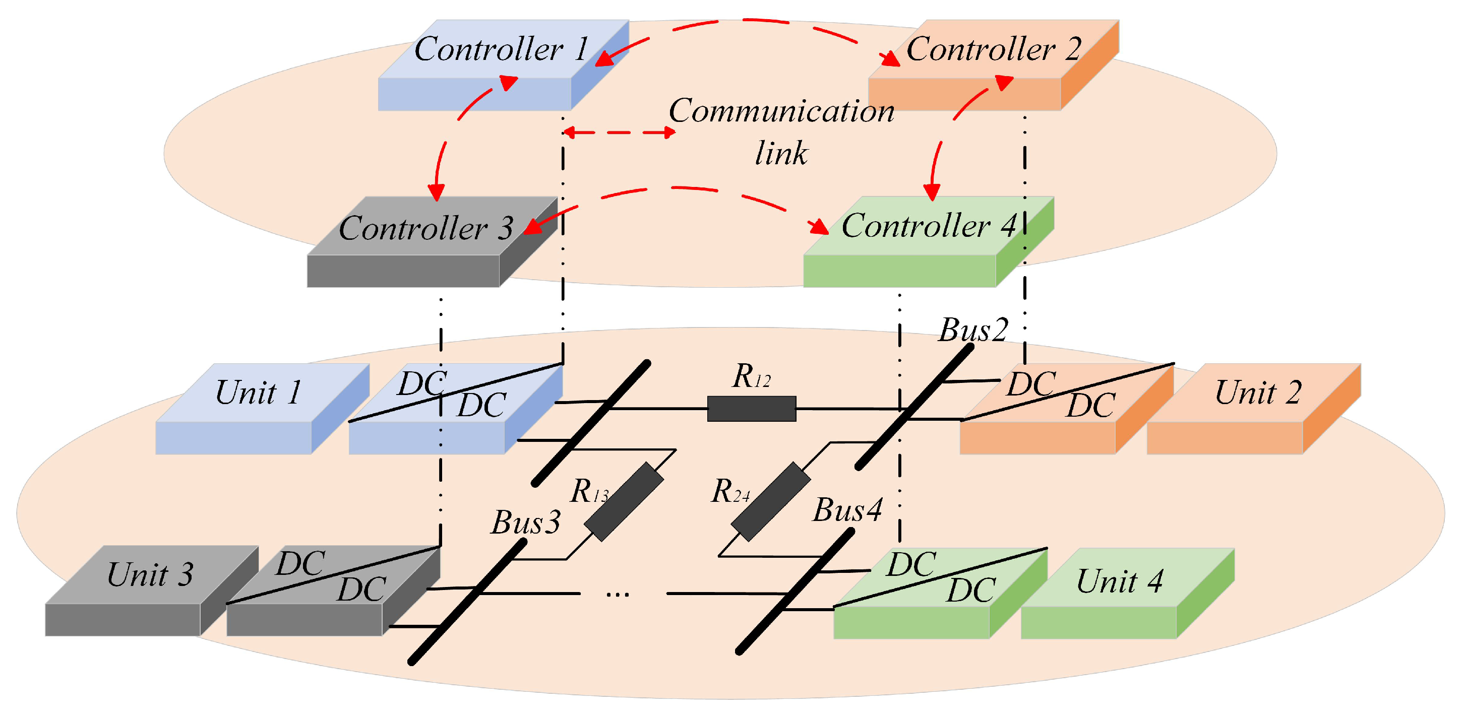
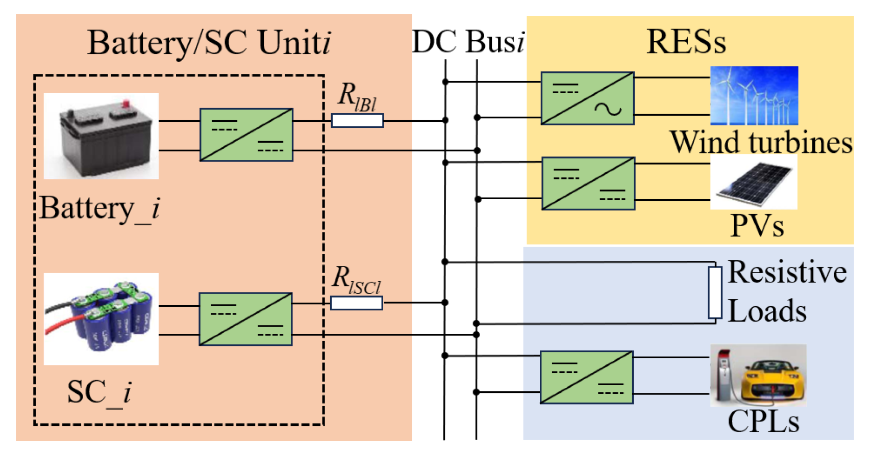
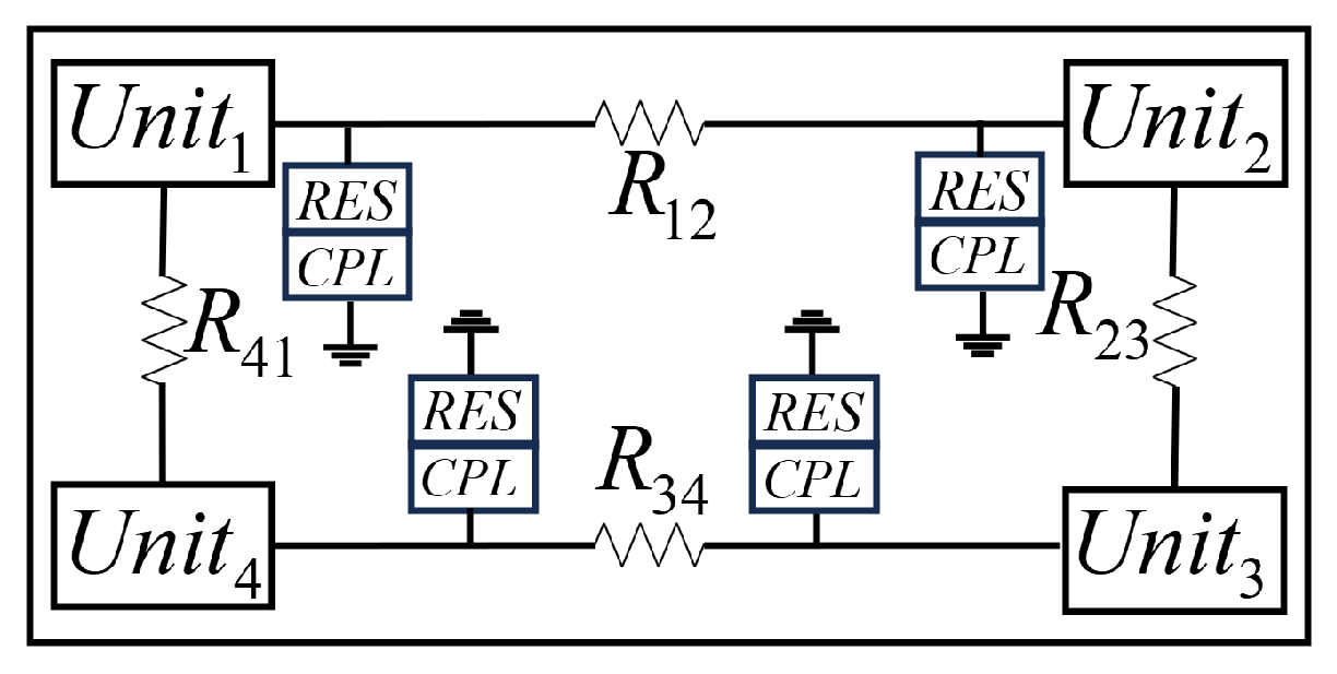
2. Problem Analysis and System Modeling

Since the multi-bus architecture can enhance system stability [19], this paper focuses on a multi-bus hybrid energy storage microgrid. The structure and controller configuration of the multi-bus HESS are illustrated in Figure 1. The schematic of the ith HES unit in the DC microgrid is illustrated in Figure 2. The communication links in the system are depicted as a graph $G=(\mathcal{N},\mathcal{E},\mathcal{A})$. $\mathcal{N}=(n_1,n_2,\dots ,n_N)$ denotes nodes and $\mathcal{E}$ represents the set of edges. $\mathcal{A}=\left[a_{ij}\right]\in R^{N\times N}$ is an adjacency matrix, $a_{ij}=1$ if a communication link exists between node i and node j, otherwise $a_{ij}=0$. $\mathcal{D}=diag\left({\iota }_i\right)\in R^{N\times N}$ denotes the degree matrix, ${\iota }_i={\sum }_{j\in N_i}{a}_{ij}$. $\mathcal{L}=\mathcal{D}-\mathcal{A}$ is the Laplacian matrix.

2.1. Nonlinearity in the Voltage–Current Relationship Caused by CPLs

To evaluate the influence of CPLs on voltage–current characteristics, the HES units are represented by the simplified configuration illustrated in Figure 3. When minor power losses are disregarded, the power equilibrium relationship can be mathematically described as:

$$P_{out}=\sum P_x=P_R+P_{CPL}-P_{RES}$$

(1)

where $x=$ BAT or SC. $P_{out}$, $P_R$, $P_{CPL}$, and $P_{RES}$ represent the output power of the ith unit, resistive load power, CPL power, and RES power, respectively.

Therefore, according to Kirchhoff’s Voltage Law, we can derive the relationship:

$$\left\{\begin{array}{cc}\hfill & C_x{\displaystyle \frac{d{v}_{out}}{dt}}=i_{in}-i_{out}\hfill \\ \hfill & i_{out}={\displaystyle \frac{v_{out}}{R}}+{\displaystyle \frac{P_{CPL}}{v_{out}}}-{\displaystyle \frac{P_{RES}}{v_{out}}}\hfill \end{array}\right.$$

(2)

where $C_x$ represents the filter capacitor for BAT or SC, $i_{out}$ is the output current from BAT or SC. Consequently, the integration of CPLs fundamentally alters the core linear correlation between output current and voltage, introducing nonlinear system behavior. This makes both traditional I–V droop control strategies and the enhanced I–V droop approach presented in [12] inadequate when CPLs exist. Additionally, standard linear PI controllers lose their ability to directly employ voltage feedback signals for maintaining system voltage stability.

However, from an alternative analytical standpoint, the following relationship can be established:

$$\left\{\begin{array}{c}{\displaystyle \frac{1}{2}}{C}_x{\displaystyle \frac{d{v}_{out}^2}{dt}}=P_{in}-P_{out}=E_x{i}_L-P_{out}\hfill \\ P_{out}={\displaystyle \frac{v_{out}^2}{R}}+P_{CPL}-P_{RES}\hfill \end{array}\right.$$

(3)

where $E_x$, $i_L$, $P_{in}$, and $P_{out}$ denote the source voltage, inductor current, input power, and output power, respectively.

Crucially, while preserving the inherent nonlinearity in voltage–current characteristics, a distinct linear proportionality manifests between power output and squared voltage magnitudes (i.e., $P\propto V^2$). This observation leads to the development of the improved P–V² droop control strategy to maintain operational voltage stability.

Given the dual operational requirements of local droop controllers to maintain bus voltage stabilization while enabling autonomous allocation of transient power to SCs and steady-state power to BATs, this study leverages the established P–V² correlation to formulate the following control framework:

$$\left\{\begin{array}{c}{\left(V_{SCi}^{ref}\right)}^2={\left(V_{busi}^{*}\right)}^2-{\displaystyle \frac{a_{SCi}}{s}}{P}_{outSCi}+u_{SC}^i\hfill \\ {\left(V_{BATi}^{ref}\right)}^2={\left(V_{busi}^{*}\right)}^2-a_{BATi}{P}_{outBATi}+u_{BAT}^i\hfill \end{array}\right.$$

(4)

where $V_{busi}^{*}$ represents the unload voltage of the ith bus; $a_{xi}$ is the droop coefficient; and $u_x^i$ denotes the secondary control signal that compensates for voltage deviations, which is determined in Section 3. $V_{xi}^{ref}$ represents the reference voltage.

According to Equation (4), the current distribution between BATs and SCs within the HES unit can be derived as follows:

$$\left\{\begin{array}{c}{P}_{outBATi}=G_{BAT}\left(s\right)P_{outi}={\displaystyle \frac{{\omega }_{BAT}}{{\omega }_{SC}s+{\omega }_{BAT}}}{P}_{outi}\hfill \\ P_{outSCi}=G_{SC}\left(s\right)P_{outi}={\displaystyle \frac{{\omega }_{SC}s}{{\omega }_{SC}s+{\omega }_{BAT}}}{P}_{outi}.\hfill \end{array}\right.$$

(5)

where ${\omega }_x={\displaystyle \frac{{\left(V_{busi}^{*}\right)}^2-{\left(V_{xi}^{ref}\right)}^2+u_x^i}{a_{xi}}}$. This control methodology fundamentally decouples the dynamics of the current distribution, as evidenced by theoretical analysis. The transfer functions $G_{BAT}\left(s\right)$ and $G_{SC}\left(s\right)$ function as low-pass and high-pass filters, respectively, thereby establishing distinct frequency-domain operational domains: BATs govern low-frequency power components, while SCs regulate high-frequency transients.

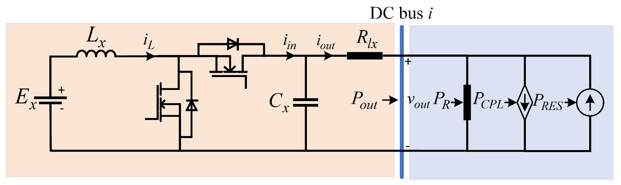
2.2. Modeling of the DC–DC Converter

Given the intrinsic involvement of DC–DC inverters in voltage/current regulation tasks during droop control implementation, this study develops a dynamic modeling framework grounded in their inductive–capacitive network characteristics. Fundamental analysis of power converter dynamics yields the following operational relationships:

$$\left\{\begin{array}{c}{L}_x{\displaystyle \frac{d{i}_{Lx}}{dt}}=E_x-(1-d_x)v_{outx}\hfill \\ C_x{\displaystyle \frac{d{v}_{outx}}{dt}}=(1-d_x)i_{Lx}-P_x/v_{outx}\hfill \end{array}\right.$$

(6)

where $d_i$ is the duty ratio of the converter.

According to Equation (6), the state-space representation of the system can be formulated as follows:

$$\left\{\begin{array}{c}{x}_{x1}={\displaystyle \frac{1}{2}}{L}_x{i}_{Lx}^2+{\displaystyle \frac{1}{2}}{C}_x{v}_{outx}^2\hfill \\ x_{x2}=E_x{i}_{Lx}\hfill \end{array}\right.$$

(7)

Differentiating the state function yields:

$$\left\{\begin{array}{c}\dot{x_{x1}}=L_x{i}_{Lx}\dot{i_{Lx}}+C_x{v}_{outx}\dot{v_{outx}}+u_{x1}\hfill \\ \dot{x_{x2}}=E_x\dot{i_{Lx}}\hfill \end{array}\right.$$

(8)

where $u_{x1}=-P_x$. If $u_{x1}$ is treated as a disturbance, the following can be derived:

$$\left\{\begin{array}{c}\dot{x_{x1}}=x_{x2}+u_{x1}\hfill \\ \dot{x_{x2}}={\vartheta }_x\hfill \end{array}\right.$$

(9)

where ${\vartheta }_x=E_x^2/L_x-(1-d_x)v_{outx}{E}_x/L_x$. Therefore, once ${\vartheta }_i$ is determined, the duty cycle of the inverter can be derived, which will be addressed in the subsequent primary controller design. From the above analysis, it can be concluded that the control objective of the primary controller is to ensure the state variable $x_{x1}$ tracks its reference signal $x_{x1}^{*}$.

$$x_{x1}^{*}={\displaystyle \frac{1}{2}}{L}_x{\left(i_{Lx}^{ref}\right)}^2+{\displaystyle \frac{1}{2}}{C}_x{\left(v_{outx}^{ref}\right)}^2,i_{Lx}^{ref}=P_x^{ref}/E_x$$

(10)

3. The Proposed Controller Design

3.1. Primary Controller Design

The extended finite-time observer (EFTO) design technique in [26] is adopted for disturbance estimation, necessitating key assumptions.

Assumption A1. 

The disturbance and its higher-order derivatives $u_{x1}$, ${\dot{u}}_{x1}$, ${\ddot{u}}_{x1}$ satisfy

$$\underset{t>0}{sup}|u_{x1}|\le {\epsilon }_0,\underset{t>0}{sup}|{\dot{u}}_{x1}|\le {\epsilon }_1,\underset{t>0}{sup}\left|{\ddot{u}}_{x1}\right|\le {\epsilon }_2$$

(11)

According to the technique in [26], in order to estimate $u_{x1}$, EFTO is designed as:

$$\left\{\begin{array}{c}\dot{x_{x10}}=x_{x2}+w_{x0},\dot{x_{x11}}=w_{x1},\dot{x_{x12}}=w_{x2}\hfill \\ w_{x0}=x_{x11}-b_0{k}^{1/3}{\mathrm{sig}}^{2/3}(x_{x10}-x_{x1})\hfill \\ w_{x1}=x_{x12}-b_1{k}^{1/2}{\mathrm{sig}}^{1/2}(x_{x11}-w_{x0})\hfill \\ w_{x2}=-b_{2}k\mathrm{sign}(x_{x12}-w_{x1})\hfill \end{array}\right.$$

(12)

where k is a positive gain to be decided and ${\mathrm{sig}}^{\lambda }\left(z\right)={\left|z\right|}^{\lambda }\mathrm{sign}\left(z\right)$. ($b_0$, $b_1$, $b_2$) are the parameters that correspond to the Horowitz polynomials, $K_j\left(s\right)=s^3+b_0{s}^2+b_{1}s+b_2$. $x_{x10}$, $x_{x11}$, $x_{x12}$ are the estimations of $x_{x1}$, $u_{x1}$, and $\dot{u_{x1}}$. The error can be obtained:

$$\left\{\begin{array}{c}{\tilde{x}}_{x1}=x_{x10}-x_{x1}={\widehat{x}}_{x1}-x_{x1}\hfill \\ {\tilde{u}}_{x1}=x_{x11}-u_{x1}={\widehat{u}}_{x1}-u_{x1}\hfill \\ {\tilde{\dot{u}}}_{x1}=x_{x12}-{\dot{u}}_{x1}={\widehat{\dot{u}}}_{x1}-{\dot{u}}_{x1}\hfill \end{array}\right.$$

(13)

where ${\widehat{x}}_{x1}$, ${\widehat{u}}_{x1}$, and ${\widehat{\dot{u}}}_{x1}$ represent the estimations of $x_{x1}$, $u_{x1}$ and ${\dot{u}}_{x1}$, respectively. Consequently, the error dynamics are formulated as follows:

$$\left\{\begin{array}{c}{\dot{\tilde{x}}}_{x1}={\tilde{u}}_{x1}-b_0{k}^{1/3}{\mathrm{sig}}^{2/3}\left({\tilde{x}}_{x1}\right)\hfill \\ {\dot{\tilde{u}}}_{x1}={\tilde{\dot{u}}}_{x1}-b_1{k}^{1/2}{\mathrm{sig}}^{1/2}\left({\tilde{u}}_{x1}-{\dot{\tilde{x}}}_{x1}\right)\hfill \\ {\dot{\tilde{\dot{u}}}}_{x1}\in -b_{2}k\mathrm{sign}\left({\tilde{\dot{u}}}_{x1}-{\dot{\tilde{u}}}_{x1}\right)+[-{\epsilon }_2,{\epsilon }_2]\hfill \end{array}\right.$$

(14)

The error dynamics described in System (14) can be stabilized within finite time, as validated in [26]. Therefore, ${\widehat{x}}_{x1}$, ${\widehat{u}}_{x1}$, and ${\widehat{\dot{u}}}_{x1}$ can converge to $x_{x1}$, $u_{x1}$ and ${\dot{u}}_{x1}$. Therefore, let ${\widehat{u}}_{x1}$ replace the actual output power, and the reference signal can be reformulated as follows:

$${\widehat{x}}_{x1}^{*}={\displaystyle \frac{1}{2}}{L}_x{\left(-{\displaystyle \frac{{\widehat{u}}_{x1}}{E_x}}\right)}^2+{\displaystyle \frac{1}{2}}{C}_x\left[{\left(V_{busi}^{*}\right)}^2+a_x{\widehat{u}}_{x1}+u_x\right]$$

(15)

The error variable is defined as $e_{x1}=x_{x1}-{\widehat{x}}_{x1}^{*}$, the Lyapunov function is given as:

$$V\left(e_{x1}\right)={\displaystyle \frac{1}{2}}{e}_{x1}^2$$

(16)

Taking the derivative of Equation (16) yields:

$$\dot{V}\left(e_{x1}\right)=e_{x1}{\dot{e}}_{x1}=e_{x1}\left(e_{x2}+{\widehat{x}}_{x2}^{*}+u_{x1}-{\dot{\widehat{x}}}_{x1}^{*}\right)$$

(17)

The another reference signal ${\dot{\widehat{x}}}_{x1}^{*}$ can be defined as:

$${\widehat{x}}_{x2}^{*}=-l_{11}{e}_{x1}-l_{12}{\mathrm{sig}}^{\lambda }\left(e_{x1}\right)-{\widehat{u}}_{x1}+{\dot{\widehat{x}}}_{x1}^{*}$$

(18)

where $l_{11}>0$, $l_{12}>0$, and $\lambda \in (0,1)$ are positive gains.

Supposing another error variable is $e_{x2}=x_{x2}-{\widehat{x}}_{x2}^{*}$, $e_{x2}$ is derived as:

$${\dot{e}}_{x2}={\vartheta }_x-{\dot{\widehat{x}}}_{x2}^{*}$$

(19)

Then, the Lyapunov function is rewritten as:

$$V(e_{x1},e_{x2})=V\left(e_{x1}\right)+{\displaystyle \frac{1}{2}}{e}_{x2}^2$$

(20)

Taking the derivative of Equation (20) yields:

$$\dot{V}(e_{x1},e_{x2})=\dot{V}\left(e_{x1}\right)+e_{x2}\left({\vartheta }_x-{\dot{\widehat{x}}}_{x2}^{*}\right)$$

(21)

Therefore, ${\vartheta }_x$ can be designed as:

$${\vartheta }_x=-e_{x1}-l_{21}{e}_{x2}-l_{22}{\mathrm{sig}}^{\lambda }\left(e_{x2}\right)+{\dot{\widehat{x}}}_{x2}^{*}$$

(22)

where $l_{21}>0$, $l_{22}>0$, and $\lambda \in (0,1)$ are positive gains.

3.2. Secondary Controller Design

$u_{xi}$ is the compensation amount decided by a secondary controller, which can be represented as:

$${\dot{u}}_x^i=\dot{({\left(V_{xi}^{ref}\right)}^2+D_{xi}{P}_{outxi})}=e_x^i$$

(23)

where $e_x^i$ is the control input and $D_{xi}={\displaystyle \frac{a_{SCi}}{s}}$ or $a_{BATi}$. To achieve precise power sharing among buses, $e_x^i$ can be designed as:

$$e_x^i=f_{xi}\left[\sum _{j\in N_{\mathrm{i}}}{a}_{ij}\left(D_{xj}\widehat{P_{outxj}}-D_{xi}\widehat{P_{outxi}}\right)\right]$$

(24)

$$\widehat{P_{outxi}}\left(t\right)=P_{outxi}\left(t_k^i\right),t\in [t_k^i,t_{k+1}^i)$$

(25)

where $t_k^i$ indicates the dynamic event-triggered time and $f_{xi}$ is the control gain.

Define $\widehat{q_{xi}}={\left(\widehat{V_{xi}^{ref}}\right)}^2+D_{xi}\widehat{P_{outxi}}$, $q_{ref}=V_{ref}^2+D{P}_{pu}$. Moreover, $D_{xi}\widehat{P_{outxi}}$ converges to a certain constant value $D{P}_{\mathrm{pu}}$ in the steady state. Then, Equation (10) can be rewritten as:

$$\stackrel{.}{q_{xi}}=f_{xi}\left(\sum _{j\in N_{\mathrm{i}}}{a}_{ij}(\widehat{q_{xj}}-\widehat{q_{xi}})\right)$$

(26)

To simplify the calculation, the error term ${\zeta }_{xi}$ is designed as:

$${\zeta }_{xi}=\sum _{j\in N_{\mathrm{i}}}{a}_{ij}(\widehat{q_{xj}}-\widehat{q_{xi}})$$

(27)

The triggering error in dynamic event-triggered communication is defined as:

$$e_{xi}^d=\widehat{q_{xi}}-q_{xi}$$

(28)

The event trigger time is generated based on the following event trigger condition

$$t_{k+1}^i=inf\left\{t>t_k^i|T_i\rangle m_i{\gamma }_i\right\}$$

(29)

where $b_i$ functions as a proportional control gain, while $T_i$ is characterized as:

$$T_i\left(t\right)={∥e_{xi}^d∥}^2-{\displaystyle \frac{\varrho \left(1-\alpha {\sum }_{j\in N_i}{a}_{ij}\right)}{{\sum }_{j\in N_i}{a}_{ij}/\alpha }}{∥{\zeta }_{xi}∥}^2$$

(30)

where $0<\varrho <1$, $0<\alpha <{\displaystyle \frac{1}{{\sum }_{j\in N_i}{a}_{ij}}}$.

The dynamic parameter ${\gamma }_i$ is an auxiliary variable that satisfies:

$$\stackrel{.}{{\gamma }_i}=-{\sigma }_i{\gamma }_i-{\beta }_i{T}_i$$

(31)

where ${\sigma }_i>0$,${\beta }_i\in [0,1]$.

4. Stability Analysis

The following lemmas are essential prerequisites for the stability analysis of the primary control layer.

Lemma 1 

([27]). Suppose that there is a Lyapunov function $V\left(\chi \right)$, ${\kappa }_1>0$, ${\kappa }_2>0$ satisfying

$$\dot{V}\left(\chi \right)\le -{\kappa }_{1}V\left(\chi \right)-{\kappa }_2{V}^{\lambda }\left(\chi \right),\forall \chi \in \mathcal{R}$$

(32)

Then, the system is finite-time stable, and the setting time Λ is bounded by

$$\mathrm{\Lambda }\le {\displaystyle \frac{ln\left(1+({\kappa }_1/{\kappa }_2)V^{\frac{\lambda +1}{2}}\left({\chi }_0\right)\right)}{{\kappa }_1(1-\lambda )}}$$

(33)

Lemma 2 

([26]). For any real numbers $a_i$ for $i=1,2,\dots ,n$ and $0<b<1$,

$$\left(\right|a_1|+|a_2|+\dots +|a_n{\left|\right)}^b\le |a_1{|}^b+|a_2{|}^b+\dots +{\left|a_n\right|}^b$$

(34)

Defining $e=(e_{x1},e_{x2})$, $\dot{V}\left(e\right)$ can be obtained:

$$\dot{V}\left(e\right)=-l_{11}{e}_{x1}^2-l_{21}{e}_{x2}^2-l_{12}|e_{x1}{|}^{\lambda +1}-l_{22}{\left|e_{x2}\right|}^{\lambda +1}+e_{x1}{\tilde{u}}_{x1}$$

(35)

Since $e_{x1}^2$, $e_{x2}^2$, $|e_{x1}{|}^{\lambda +1}$ and $|e_{x2}{|}^{\lambda +1}$ are non-negative,

$$\dot{V}\left(e\right)\le e_{x1}{\tilde{u}}_{x1}\le 0.5\left(\right|e_{x1}{|}^2+|{\tilde{u}}_{x1}{|}^2)\le V\left(e\right)+\mathrm{\Delta }$$

(36)

where $\mathrm{\Delta }=max\left(0.5\right|{\tilde{u}}_{x1}{|}^2)$.

Since ${\tilde{u}}_{x1}$ is bounded, $\mathrm{\Delta }$ remains bounded as well. For $[0,{\mathrm{\Lambda }}_s]$, Equation (36) can be solved as:

$$V\left(e\right)\le [V\left(e_0\right)+\mathrm{\Delta }]e^t-\mathrm{\Delta }\le [V\left(e_0\right)+\mathrm{\Delta }]e^{{\mathrm{\Lambda }}_s}-\mathrm{\Delta }$$

(37)

where $e_0$ denotes the initial value of e. Equation (37) indicates that the boundedness of the HESS is guaranteed.

Based on Equation (35), the following relationship is given as:

$$\dot{V}\left(e\right)\le -l_{11}{e}_{x1}^2-l_{21}{e}_{x2}^2-l_{12}|e_{x1}{|}^{\lambda +1}-l_{22}|e_{x2}{|}^{\lambda +1}+|e_{x1}\left|\right|{\tilde{u}}_{x1}|$$

(38)

Then, the following inequalities can be derived as:

$$\begin{array}{c}\hfill \dot{V}\left(e\right)\le -l_{11}{e}_{x1}^2-l_{21}{e}_{x2}^2-\left(l_{12}-|{\tilde{u}}_{x1}|/|e_{x1}{|}^{\lambda }\right)|e_{x1}{|}^{\lambda +1}-l_{22}{\left|e_{x2}\right|}^{\lambda +1}\end{array}$$

(39)

According to Equation (39) and Lemma 2, if $|e_{x1}{|}^{\lambda }>\left|{\tilde{u}}_{x1}\right|/l_{12}$, we can obtain:

$$\begin{array}{cc}\hfill \dot{V}\left(e\right)& \le -\phi \left(e_{x1}^2+e_{x2}^2\right)-\varphi \left(e_{x1}^{\lambda +1}+e_{x2}^{\lambda +1}\right)\hfill \\ \hfill & \le -\phi \left(e_{x1}^2+e_{x2}^2\right)-\varphi {\left(e_{x1}^2+e_{x2}^2\right)}^{{\displaystyle \frac{\lambda +1}{2}}}\hfill \\ \hfill & =-K_{1}V\left(e\right)-K_2{V}^{{\displaystyle \frac{\lambda +1}{2}}}\left(e\right),\hfill \end{array}$$

(40)

where $\phi =\min \{l_{11},l_{21}\}={\displaystyle \frac{K_1}{2}}$ and $\varphi =\min \{l_{12}-|{\tilde{u}}_{x1}|/|e_{x1}{|}^{\lambda },l_{22}\}={\displaystyle \frac{K_2}{2^{\lambda +0.5}}}$.

According to Equation (39) and Lemma 1, HESS will be captured by the following domain.

$$|e_{x1}|\le (|{\tilde{u}}_{x1}{|/l_{12})}^{1/\lambda }$$

(41)

Based on the aforementioned analysis and Assumption 1, the boundedness of $\phi$ and $\varphi$ can be ensured through appropriate parameter tuning, thereby achieving stability of the primary controller.

Then, the stability proof for the secondary controller is conducted. Based on Equation (26), denote $\delta$ as

$${\delta }_x=q_x-q_x^{\mathrm{ref}}$$

(42)

Combining Equations (26), (28), and (42) yields

$$\stackrel{.}{{\delta }_x}=-f_x\mathcal{M}({\delta }_x+e_x^d)$$

(43)

where ${\delta }_x={[{\delta }_{x1},{\delta }_{x2},\dots ,{\delta }_{xN}]}^T$, $e_x^d={[e_{x1}^d,e_{x2}^d,\dots ,e_{xN}^d]}^T$. Similarly, based on (27), it can be obtained as

$${\zeta }_x=-\mathcal{M}({\delta }_x+e_x^d)$$

(44)

where ${\zeta }_x={[{\zeta }_{x1},{\zeta }_{x2},\dots ,{\zeta }_{xN}]}^T$.

The following Lyapunov function is written as

$$V={\displaystyle \frac{1}{2}}{\delta }_x^T\mathcal{M}{\delta }_x$$

(45)

Taking the derivative of Equation (45) gives

$$\dot{V}={\delta }_x^T\mathcal{M}\dot{{\delta }_x}$$

(46)

Substituting Equation (44) can yield

$$\dot{V}=-f_x{\delta }_x^T{\mathcal{M}}^2({\delta }_x+e_x^d)$$

(47)

$\mathcal{M}$ is reversible, then, by substituting Equation (44) into Equation (47), it yields:

$$\dot{V}=-f_x{\zeta }_x^T\mathcal{M}{e}_x^d-f_x{\zeta }_x^T{\zeta }_x=-f_x{\zeta }_x^T\mathcal{M}{e}_x^d-f_x{\parallel {\zeta }_x\parallel }^2$$

(48)

Equation (48) can be extended as:

$$\begin{array}{cc}\hfill \dot{V}& =-f_x\left[\sum _{i=1}^N{\parallel {\zeta }_{xi}\parallel }^2-\sum _{i=1}^N\sum _{j\in N_i}{a}_{ij}{\zeta }_{xi}{e}_{xi}^d+\sum _{j=1}^N\sum _{j\in N_i}{a}_{ij}{\zeta }_{xi}{e}_{xj}^d\right]\hfill \end{array}$$

(49)

Noting that

$$x^{T}y\le {\displaystyle \frac{\alpha }{2}}{\parallel x\parallel }^2+{\displaystyle \frac{1}{2\alpha }}{\parallel y\parallel }^2,\alpha >0$$

(50)

The upper bound of Equation (49) can be derived as

$$\begin{array}{c}\hfill \dot{V}\le -f_x\sum _{i=1}\parallel {\zeta }_{xi}{\parallel }^2+f_x\sum _{i=1}^N\sum _{j\in N_i}{a}_{ij}\alpha \parallel {\zeta }_{xi}{\parallel }^2+f_x\sum _{i=1}^N\sum _{j\in N_i}{a}_{ij}{\displaystyle \frac{1}{2\alpha }}\parallel e_{xi}^d{\parallel }^2+f_x\sum _{i=1}^N\sum _{j\in N_i}{a}_{ij}{\displaystyle \frac{1}{2\alpha }}{\parallel e_{xj}^d\parallel }^2\end{array}$$

(51)

Since the topology diagram in this study is undirected, then

$$\sum _{i=1}^N\sum _{j\in N_i}{a}_{ij}\parallel e_{xj}^d{\parallel }^2=\sum _{i=1}^N\sum _{j\in N_i}{a}_{ij}{\parallel e_{xi}^d\parallel }^2$$

(52)

Substituting (52) into (51) yields

$$\dot{V}=f_x\sum _{i=1}^N\left(\alpha \sum _{j\in N_i}{a}_{ij}-1\right)\parallel {\zeta }_{xi}{\parallel }^2+f_x\sum _{i=1}^N\left({\displaystyle \frac{1}{\alpha }}\sum _{j\in N_i}{a}_{ij}\right){\parallel e_x^d\parallel }^2$$

(53)

Assuming that

$$0<\alpha <{\displaystyle \frac{1}{{\sum }_{j\in N_i}{a}_{ij}}}$$

(54)

$${∥e_x^d∥}^2\le {\displaystyle \frac{\varrho (1-\alpha {\sum }_{j\in N_i}{a}_{ij})}{{\sum }_{j\in N_i}\frac{a_{ij}}{\alpha }}}{∥{\zeta }_{xi}∥}^2$$

(55)

Then, the following condition can be obtained

$$\left(\sum _{j\in N_i}{\displaystyle \frac{a_{ij}}{\alpha }}\right){∥e_x^d∥}^2+\left(\alpha \sum _{j\in N_i}{a}_{ij}-1\right){∥{\zeta }_{xi}∥}^2\le 0$$

(56)

which implies $\dot{V}<0$.

Then, the dynamic parameter ${\vartheta }_i$ is introduced, and it can be derived as

$${\gamma }_i\left(t\right)\ge {\gamma }_i\left(0\right)e^{-\left({\sigma }_i+m_i{\beta }_i\right)t}>0$$

(57)

Then, the Lyapunov function with the dynamic variable can be expressed as

$$V_d=V+\sum _{i=1}^N{\gamma }_i\left(t\right)$$

(58)

$$\begin{array}{cc}\hfill \dot{V_d}& =\dot{V}+\sum _{i=1}^N{\dot{\gamma }}_i=\dot{V}-\sum _{i=1}^N{\sigma }_i{\gamma }_i+\sum _{i=1}^N{\beta }_i({\iota }_i\parallel {\zeta }_{xi}{\parallel }^2-\parallel e_{xi}^d{\parallel }^2)\hfill \\ & \le \sum _{i=1}^N({∥e_{xi}^d∥}^2-{\iota }_i{∥{\zeta }_{xi}∥}^2)-\sum _{i=1}^N{\sigma }_i{\gamma }_i+\sum _{i=1}^N{\beta }_i({\iota }_i{∥{\zeta }_{xi}∥}^2-{∥e_{xi}^d∥}^2)\hfill \\ \hfill & \le \sum _{i=1}^N\left[m_i\left(1-{\beta }_i\right)-{\sigma }_i\right]{\gamma }_i\hfill \end{array}$$

(59)

where ${\iota }_i={\displaystyle \frac{\varrho \left(1-\alpha {\sum }_{j\in N_i}{a}_{ij}\right)}{{\sum }_{j\in N_i}{a}_{ij}/\alpha }}$. If ${\sigma }_i$, ${\beta }_i$, $m_i$ can be properly selected, ${\gamma }_i>0$, then $m_i\left(1-{\beta }_i\right)-{\sigma }_i<0$. i.e., $\dot{V_d}<0$. Therefore, the system is stable.

5. Simulation and Experimental Results

5.1. Simulation Results

This section comprehensively evaluates the proposed multi-bus HESS control framework in terms of robustness and operational efficacy. The system architecture, depicted in Figure 4, provides a detailed schematic of the multi-bus configuration and the interconnection logic among HES units.

To verify the efficacy of the developed control scheme, dynamic operating scenarios involving load transients and power demand fluctuations are simulated. Specific test cases encompass the integration of CPLs, step variations in resistive load impedances, and time-dependent power reference adjustments for CPLs. The central objective is to analyze the controller’s capacity to regulate power distribution across HES units and achieve voltage stabilization under transient disturbances. Key operational parameters for the HES units and control design specifications are summarized in

Table 1. Simulation parameters.

Symbol	Quantity	Nominal Value
$V_{busi}^{*}$	bus voltage reference value	300 V
$E_{SC}$	SC voltage reference value	150 V
$E_B$	Battery voltage reference value	150 V
$f_s$	switching frequency	2 KHz
L	inductance	0.8 mH
C	capacitance	2.2 mF
$R_{ij}$	HES units’ line impedance	$R_{12}$ = 0.3 $\mathrm{\Omega }$
		$R_{23}$ = 0.6 $\mathrm{\Omega }$
		$R_{34}$ = 0.8 $\mathrm{\Omega }$
		$R_{41}$ = 0.7 $\mathrm{\Omega }$
$R_{Loadi}$	Resistive Load	$R_{Load1}$ = 100 $\mathrm{\Omega }$
		$R_{Load2}$ = 50 $\mathrm{\Omega }$
		$R_{Load3}$ = 80 $\mathrm{\Omega }$
		$R_{Load4}$ = 40 $\mathrm{\Omega }$
$a_{SC}$	Virtual Resistance Coefficient	$a_{SC1}=0.4\pi$, $a_{SC2}=0.8\pi$
		$a_{SC3}=0.4\pi$, $a_{SC4}=0.8\pi$
$a_{BAT}$	Virtual Inductance Coefficient	$a_{BAT1}=0.4$, $a_{BAT2}=0.8$
		$a_{BAT3}=0.4$, $a_{BAT4}=0.8$
$b_0$		3
$b_1$		3
$b_2$		1
k	Primary control gains	2000
$l_{11}$		2000
$l_{12}$		10,000
$\lambda$		0.5
$f_{x}i$	error gain	20
${\sigma }_i$		8
${\beta }_i$		1
$m_i$	Dynamic Event-triggered Control	1.5
$\varrho$		0.5
$\alpha$		0.2

.

The analysis demonstrates that precise power sharing among HES units is validated under a 2:1:2:1 output current ratio, with verification carried out through sequential load disturbances to evaluate the adaptability of the control strategy to plug-and-play. At $t=5$ s, the first CPL undergoes a sudden increase in power of 1800 W, followed by a reduction of 1800 W at $t=10$ s. Subsequently, the third RES reduces its power demand by 900 W at $t=15$ s, and a $40\mathrm{\Omega }$ resistive load is connected to $R_{Load4}$ in parallel at $t=20$ s. The load on the fourth bus is completely disconnected due to a fault at $t=25$ s. As illustrated in Figure 5, the proposed control strategy achieves accurate power sharing across heterogeneous line impedances, resistive loads, and CPL capacities by dynamically adjusting voltage-shifting values. The output currents of the first and third units consistently maintain half the magnitude of the second and fourth battery units, confirming the predefined ratio. Figure 6 further validates asymptotic voltage regulation, because the voltage of each bus remains approximately 300 V. Additionally, Figure 7 highlights the SC’s transient response superiority, exhibiting faster dynamics compared to batteries during disturbances, while batteries exclusively supply steady-state power. Figure 8 shows the trigger timing diagram of the four units. These results collectively affirm the enhanced transient performance and stability of the primary control framework for multi-bus HESS applications.

To demonstrate the superiority of the control strategy proposed in this paper, we compare it with the P–V² control strategy in [13], which is flawed as it still relies on the linear V-I relationship to generate the voltage reference signal. We increased the CPL power demand in three steps, each by 1800 W. As shown in Figure 9, the strategy proposed in [13] becomes unstable when the total demand reaches 5400 W. However, as illustrated in Figure 10, our proposed strategy maintains stability under the same conditions.

5.2. Experimental Results

In this section, Hardware-in-the-Loop (HIL) experiments using the StarSim real-time simulator are conducted to verify the effectiveness of the proposed control strategy. In this simulation experiment, the controllers are fully deployed within the DSP (TMS320F28335), while the remaining components of the system are simulated in the HIL simulator. The system architecture is shown in Figure 11.

Since the primary objectives of this study are to eliminate the effects of CPLs, achieve autonomous power distribution, and realize proportional power sharing among multiple buses, the experimental scenario is configured as follows: At t = 5 s, the CPL power demand on the first bus undergoes a step increase of 1800 W, while other parameters remain identical to the simulation case. The proposed control strategy is implemented from the initial operation stage. Figure 12 displays the bus voltage waveforms with a target value of 300 V, where experimental results confirm that all four bus voltages deviate within 2% of the target. As shown in Figure 13, the output currents of each unit maintain an approximately 2:1:2:1 proportional distribution, demonstrating successful proportional current sharing among different buses under the proposed control strategy. Following the increased CPL power demand, Figure 14 reveals that the control scheme achieves transient power handling by the supercapacitor (SC)—with its output approaching zero during steady-state—while the battery (BAT) supplies steady-state power, effectively leveraging the transient characteristics of the hybrid energy storage system.

6. Conclusions

This paper investigates power sharing in multi-bus DC microgrids with hybrid energy storage systems. Unlike existing studies, we propose an enhanced P–V² droop control method at the primary control layer that replaces fixed coefficients with virtual conductance. This approach achieves autonomous decoupling of steady-state and transient power demands while eliminating adverse effects of CPLs, effectively ensuring bus voltage stability. Subsequently, a secondary control strategy is developed to realize current sharing among multiple buses, incorporating a dynamic event-triggered communication mechanism to reduce the system communication burden. Simulation and experimental results validate the effectiveness and robustness of the proposed control strategy.

Given that our control approach still relies on foundational modeling—where inherent simplifications may compromise physical representation fidelity—future research will prioritize data-driven and artificial intelligence technologies to reduce dependence on physics-based models in multi-bus DC energy storage system control.

References

1. Wang, R.; Sun, Q.; Hu, W.; Xiao, J.; Zhang, H.; Wang, P. Stability-Oriented Droop Coefficients Region Identification for Inverters within Weak Grid: An Impedance-Based Approach. IEEE Trans. Syst. Man Cybern. Syst. 2021, 51, 2258–2268. [Google Scholar] [CrossRef]
2. Zhang, R.; Wang, S.; Ma, J.; Jiang, Y.; Wang, P.; Liu, T.; Yang, Y. An Asymmetric Hybrid Phase-Leg Modular Multilevel Converter With Small Volume, Low Cost, and DC Fault-Blocking Capability. IEEE Trans. Power Electron. 2025, 40, 5336–5351. [Google Scholar] [CrossRef]
3. Zhang, X.; Wang, B.; Zhou, Y.; Zhang, Y.; Ukil, A. An Event-Triggered Deadbeat Control Considering Dynamic Power Loss Compensation for Hybrid Energy Storage System. IEEE Trans. Ind. Electron. 2023, 70, 6844–6855. [Google Scholar] [CrossRef]
4. Kwon, M.; Choi, S. Control Scheme for Autonomous and Smooth Mode Switching of Bidirectional DC–DC Converters in a DC Microgrid. IEEE Trans. Power Electron. 2018, 33, 7094–7104. [Google Scholar] [CrossRef]
5. Kotra, S.; Mishra, M.K. Design and Stability Analysis of DC Microgrid With Hybrid Energy Storage System. IEEE Trans. Sustain. Energy 2019, 3, 1603–1612. [Google Scholar] [CrossRef]
6. Manandhar, U.; Ukil, A.; Gooi, H.B.; Tummuru, N.R.; Kollimalla, S.K.; Wang, B.; Chaudhari, K. Energy management and control for grid connected hybrid energy storage system under different operating modes. IEEE Trans. Smart Grid. 2019, 10, 1626–1636. [Google Scholar] [CrossRef]
7. Tummuru, N.R.; Mishra, M.K.; Srinivas, S. Dynamic energy management of renewable grid integrated hybrid energy storage system. IEEE Trans. Ind. Electron. 2015, 62, 7728–7737. [Google Scholar] [CrossRef]
8. Liu, B.; Zhuo, F.; Zhu, Y.; Yi, H. System operation and energy management of a renewable energy-based dc micro-grid for high penetration depth application. IEEE Trans. Smart Grid. 2015, 6, 1147–1155. [Google Scholar] [CrossRef]
9. Cohen, I.J.; Wetz, D.A.; McRee, B.J.; Dong, Q.; Heinzel, J.M. Fuzzy logic control of a hybrid energy storage module for use as a high rate prime power supply. IEEE Trans. Dielectr. Electr. Insul. 2017, 24, 3887–3893. [Google Scholar] [CrossRef]
10. Feng, X.; Gooi, H.; Chen, S. Hybrid energy storage with multimode fuzzy power allocator for pv systems. IEEE Trans. Sustain. Energy 2014, 6, 389–397. [Google Scholar] [CrossRef]
11. Xu, Q.; Xiao, J.; Wang, P.; Pan, X.; Wen, C. A decentralized control strategy for autonomous transient power sharing and state-of-charge recovery in hybrid energy storage systems. IEEE Trans. Sustain. Energy 2017, 8, 1443–1452. [Google Scholar] [CrossRef]
12. Wang, Z.; Wang, P.; Jiang, W.; Wang, P. A Decentralized Automatic Load Power Allocation Strategy for Hybrid Energy Storage System. IEEE Trans. Energy Convers. 2021, 36, 2227–2238. [Google Scholar] [CrossRef]
13. Jiang, W.; Wang, Z.; Wang, J.; Zhang, X.; Wang, P. Decentralized Autonomous Energy Management Strategy for Multi-Paralleled Hybrid Energy Storage Systems in the DC Microgrid With Mismatched Line Impedance. IEEE Trans. Sustain. Energy 2024, 15, 1114–1126. [Google Scholar] [CrossRef]
14. Herrera, L.; Zhang, W.; Wang, J. Stability Analysis and Controller Design of DC Microgrids with Constant Power Loads. IEEE Trans. Smart Grid 2017, 8, 881–888. [Google Scholar]
15. Wu, M.; Lu, D.D.C. A Novel Stabilization Method of LC Input Filter with Constant Power Loads Without Load Performance Compromise in DC Microgrids. IEEE Trans. Ind. Electron. 2015, 62, 4552–4562. [Google Scholar] [CrossRef]
16. Cespedes, M.; Xing, L.; Sun, J. Constant-Power Load System Stabilization by Passive Damping. IEEE Trans. Power Electron. 2011, 26, 1832–1836. [Google Scholar] [CrossRef]
17. Lu, X.; Sun, K.; Guerrero, J.M.; Vasquez, J.C.; Huang, L.; Wang, J. Stability Enhancement Based on Virtual Impedance for DC Microgrids with Constant Power Loads. IEEE Trans. Smart Grid 2015, 6, 2770–2783. [Google Scholar] [CrossRef]
18. Narm, H.G.; Eren, S.; Karimi-Ghartemani, M. A Robust Controller with Integrated Plant Dynamics for Constant Power Loads in DC Microgrid. IEEE Trans. Power Electron. 2023, 38, 4419–4429. [Google Scholar] [CrossRef]
19. Zhai, M.; Sun, Q.; Wang, R.; Wang, B.; Liu, S.; Zhang, H. Fully Distributed Fault-Tolerant Event-Triggered Control of Microgrids Under Directed Graphs. IEEE Trans. Netw. Sci. Eng. 2022, 9, 3570–3579. [Google Scholar] [CrossRef]
20. Yang, Q.; Jiang, L.; Zhao, H.; Zeng, H. Autonomous Voltage Regulation and Current Sharing in Islanded Multi-Inverter DC Microgrid. IEEE Trans. Smart Grid 2018, 9, 6429–6437. [Google Scholar] [CrossRef]
21. Nasirian, V.; Moayedi, S.; Davoudi, A.; Lewis, F.L. Distributed Cooperative Control of DC Microgrids. IEEE Trans. Power Electron. 2015, 30, 2288–2303. [Google Scholar] [CrossRef]
22. Jinfeng, C.; Ke, J.; Zhenwen, X.; Rui, Z. Voltage Control Strategy of DC Microgrid Based on Discrete Consensus Algorithm. Zhejiang Electr. Power 2019, 38, 65–71. [Google Scholar]
23. Liu, X.K.; He, H.; Wang, Y.W.; Xu, Q.; Guo, F. Distributed Hybrid Secondary Control for a DC Microgrid via Discrete-Time Interaction. IEEE Trans. Energy Convers. 2018, 33, 1865–1875. [Google Scholar] [CrossRef]
24. Guo, F.; Xu, Q.; Wen, C.; Wang, L.; Wang, P. Distributed Secondary Control for Power Allocation and Voltage Restoration in Islanded DC Microgrids. IEEE Trans. Sustain. Energy 2018, 9, 1857–1869. [Google Scholar] [CrossRef]
25. Zhang, H.; Han, J.; Wang, Y.; Jiang, H. H Consensus for Linear Heterogeneous Multiagent Systems Based on Event-Triggered Output Feedback Control Scheme. IEEE Trans. Cybern. 2019, 49, 2268–2279. [Google Scholar] [CrossRef]
26. Huang, X.; Lin, W.; Yang, B. Global Finite-Time Stabilization of a Class of Uncertain Nonlinear Systems. Automatica 2005, 41, 881–888. [Google Scholar] [CrossRef]
27. Yu, S.; Yu, X.; Shirinzadeh, B.; Man, Z. Continuous Finite-Time Control for Robotic Manipulators with Terminal Sliding Mode. Automatica 2005, 41, 1957–1964. [Google Scholar] [CrossRef]
Figure 1. The structure of the multi-bus HESS.
Mathematics 13 02001 g001
Figure 2. The typical paralleled battery/SC HES unit with CPLs.
Mathematics 13 02001 g002
Figure 3. The simplified structure of the HES unit.
Mathematics 13 02001 g003
Figure 4. The communication scheme of the multi-bus HESS.
Mathematics 13 02001 g004
Figure 5. Output current of each unit in the simulation.
Mathematics 13 02001 g005
Figure 6. Output voltage of each bus in the simulation.
Mathematics 13 02001 g006
Figure 7. Current distribution of the third unit in the simulation.
Mathematics 13 02001 g007
Figure 8. The trigger timing diagram (From top to bottom: Unit 1 to Unit 4).
Mathematics 13 02001 g008
Figure 9. The other control strategy.
Mathematics 13 02001 g009
Figure 10. The proposed control strategy.
Mathematics 13 02001 g010
Figure 11. The structure of the experiment test.
Mathematics 13 02001 g011
Figure 12. Output voltage of each bus in the experiment.
Mathematics 13 02001 g012
Figure 13. Output current of each bus in the experiment.
Mathematics 13 02001 g013
Figure 14. Current distribution of the first unit in the experiment.
Mathematics 13 02001 g014