Abstract
The problem of time series determinism measurement is investigated. It is shown that a deep learning model can be used as a determinism measure of a time series. Three distinct time series classes were utilised to verify the feasibility of differentiating deterministic time series: deterministic, deterministic with noise, and stochastic. The LSTM model was constructed for each time series, and its features were thoroughly investigated. The findings of this study demonstrate a strong correlation between the root mean square error (RMSE) of the trained models and the determinism of a time series.
MSC:
94A17; 91B82; 91B84
1. Introduction
The scientific approach to studying nature is predicated on identifying laws, rules, and relationships that describe observed phenomena. Within time series analysis, the forecast is one of the frequently raised issues. Therefore, the existence of a function that governs the evolution of the system is expected, and within this work, it is considered the determinism of the system. It is acknowledged that the collected data (or measurement results) are inherently imperfect. In addition to the deterministic component, these data generally contain a stochastic element (i.e., a noise) related to the nature of the phenomenon under investigation, the quality of the experiment, and the data collection process. Consequently, numerous methodologies have been developed to determine the stochasticity of the data. The entropy-based methods are the most frequently used (and the best known). Information entropy, in particular, encompasses the Shannon entropy, Rényi entropy, Tsallis entropy, Theil index, and q-Theil index, among the most frequently employed methods [1,2,3,4,5]. Other approaches to the time series randomness are the strictly statistical methods, i.e., randomness statistical tests [6,7]. The predictability problem is associated with the signal-to-noise ratio and the analysis of chaotic systems, for example, the use of Lyapunov exponents [8]. Correlations can be local or long-range, and in addition to correlograms, Hurst exponents can be estimated to measure long-range correlations [9,10,11]. A commonality among the aforementioned methods is that they are designed to investigate specific features and do not provide a comprehensive answer to the determinism of the observed data. A more general approach is, therefore, required. This issue can be further articulated through a time series model. This issue is of fundamental importance, superseding the estimation of any of the aforementioned parameters. All possible characteristics can be estimated if the time series model is known. Despite advances in the time series models [12,13,14], no general methods can be applied. Each of the time series models has to be fitted individually, so failure of fitting does not mean that there is no other model that can explain the data. Therefore, the approach based on the time series model cannot be used as a determinism measure.
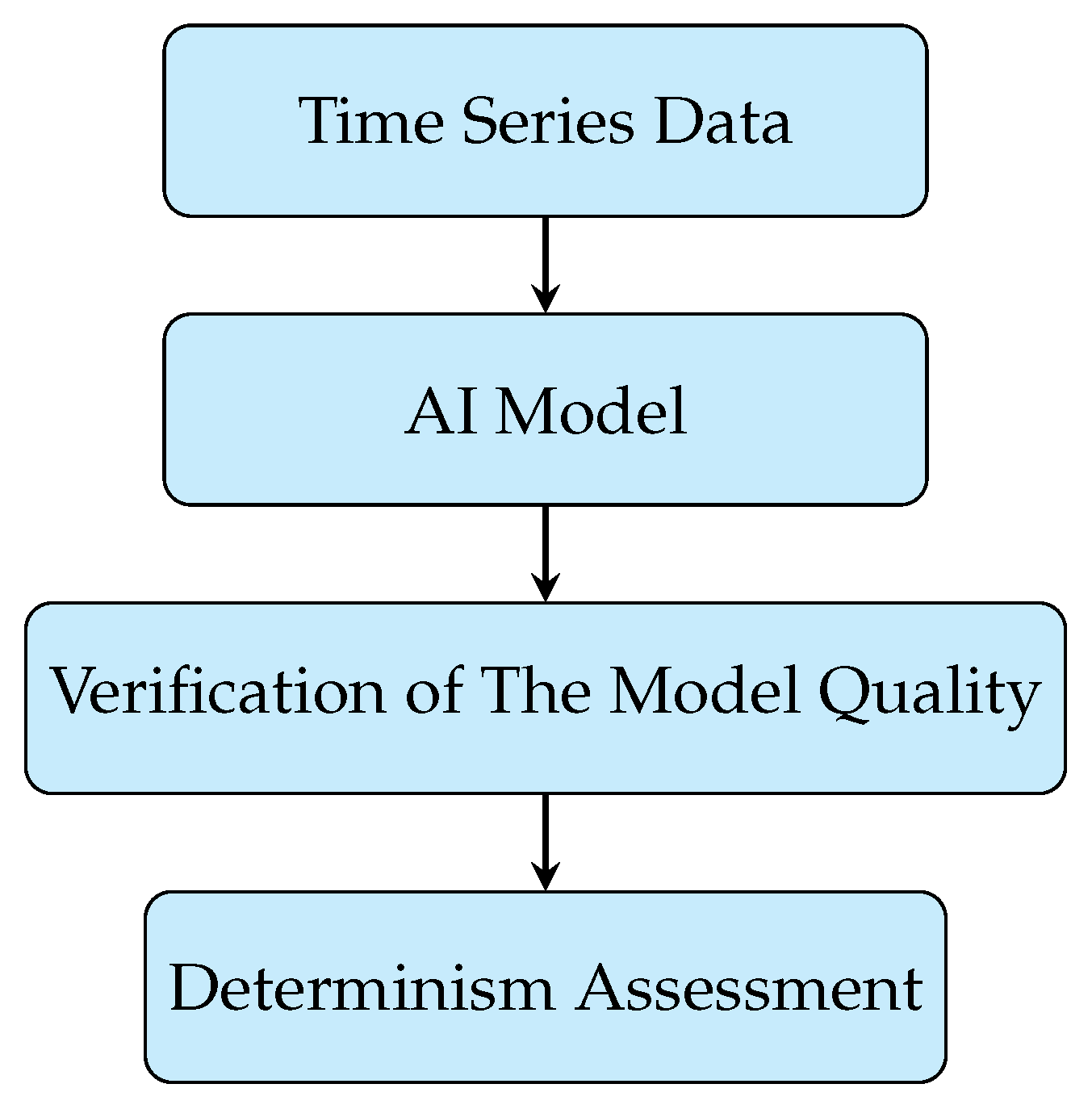
However, deep learning methods have recently allowed stating a more general method of the determinism estimation of a time series. Deep learning methods are, in fact, algorithms that are deterministic on one side and capable of being trained on the data provided. The quality of the trained model depends on several factors. However, one key feature is the existence of some deterministic patterns among the data discovered during the training stage. Of course, the model is not always satisfactory. Besides the possible mistakes in the model design, the main reason is the randomness of the analysed data. This feature allows designing a more general tool than the existing time series models for the determinism measure method. The main idea of the proposed methods is to use the quality of the trained model as a measure of the determinism of the time series. The capacity of AI models to reconstruct a wide range of time series suggests the potential for verifying the determinism of the analysed data. In this study, a novel method for assessing determinism is proposed. This method is based on the quality of the AI model trained on the time series data. It is hypothesised that highly deterministic time series will be reconstructed with high accuracy. In contrast, models trained on stochastic time series will demonstrate poor concordance with the time series. Due to the inherent characteristics of AI modelling, it is not feasible to provide a mathematical proof of the quality of the methods. The scheme of the proposed approach is presented in Figure 1. The discussion of the possible AI models and reasoning for the model choice are provided in Section 2. This paper verifies the possibility of establishing such a measure of determinism of the time series. The hypothesis is verified on the chosen examples and is performed in three classes of models: (i) deterministic time series models with a stochastic component; (ii) deterministic systems—however, in this case, the chaotic models will be used; (iii) real, stochastic models.
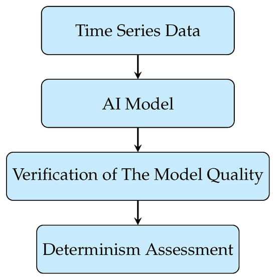
Figure 1.
The schematic presentation of the AI-based determinism assessment algorithm.
The autoregressive time series AR(p) will be used as the first class (i) examples. The primary advantage of AR(p) models is that, in addition to their purely deterministic component, they possess a stochastic component, thereby regulating the noise level. The Lorentz Attractor will represent the second class (ii). This is a deterministic system, yet it exhibits chaotic solutions. The system’s unpredictability, stemming from its sensitivity to initial conditions, challenges the conventional notion of determinism. Finally, the financial time series represent stochastic time series (iii) despite significant effort of scholars resulting in the observation of deterministic signs such as trends, seasonality, log-periodicity, long correlations, multifractality, etc. There is no clear and broadly accepted deterministic model of financial time series. Even the trends can be explained as random walks with a nonzero mean. Of course, there are obvious external factors that influence some of the financial time series (e.g., day and night periodicity in electricity demand or other feature, see, e.g., [15]). However, at present, reliable forecasting is difficult, particularly if the only information is the past data without external information. Therefore, the financial time series were chosen as an example of stochastic time series.
2. AI Time Series Models
Several classes of AI models can be used to analyse the determinism of data. Of particular note are natural language processing (NLP) models, which have recently garnered significant popularity. These models are founded upon the principle of encoder models. The primary advantage of these models lies in their capacity to capture the essential features of the input data. The encoders’ primary function is converting the input data into a numerical representation, which can subsequently be utilised to reconstruct or generate analogous data. The application of these encoder models is extensive, encompassing a wide range of disciplines including natural language processing, pattern recognition, and graph recognition [16,17]. However, this study focuses on the analysis of time series data.
The second category comprises recurrent neural networks (RNNs) [18,19,20], which have been defined for processing sequential data and are frequently employed for time series forecasting, including applications such as weather and energy production (see [21,22]). Recurrent neural networks (RNNs) can retain previous inputs, thereby enabling the capture of correlations among data points.
The long short-term memory (LSTM) model, as proposed in [23], can be regarded as a refinement of the RNN model, endowed with the capacity to retain information over extended periods. It is acknowledged that particular forecasting time series may encompass spatial challenges or exhibit patterns; for instance, energy forecasting may be contingent on a specific region. In such cases, the convolutional neural network (CNN) is employed (see [24,25]). In the present study, the LSTM model will be used to assess the determinism level of the input data.
A comprehensive overview of recurrent neural networks (RNNs) and long short-term memory (LSTM) can be found in [26,27,28]. The key elements of the RNN model are layers and the gates which control the flow of information between layers. In contrast to the RNN, the LSTM possesses an internal memory and multiplicative gates. The LSTM architecture employs three distinct types of gates: the input gate, which controls the information added to the memory cell; the forget gate, which determines the information to be removed from the memory cell; and the output gate, which controls the output from the memory cell.
The LSTM detailed description can be found in the literature, e.g., [26,27,28], so only the key elements are presented here. Let the time series be denoted as . Typically, is considered an N-dim variable, thus facilitating multivariate time series analysis. However, it should be noted that the present research will be constrained to one-dimensional variables. The output is the corresponding predicted value , where L is the horizon of the prediction. In addition to input and output states, the system encompasses data from hidden layers, denoted by . The matrices and denote learned weights and biases, while and represent the cell state and the candidate layer, respectively. The LSTM layer processes information at each step, calculating a cell state and a hidden state, utilising the following equations
where ∘ denotes pointwise multiplication, and are the forget and input gates, respectively, as shown in Equations (4) and (6). At Equation (1) the standard tanh function was used as the activation function. However, alternative activation functions are used in various applications, see, for example, refs. [29,30]. Naturally, a proper choice of activation function can increase the quality of the fitted model, and we believe that optimisation methods will be developed. However, the main goal is to demonstrate the ability of determinism assessment, so the approach of the universal model (with a chosen activation function) is used. However, if the optimisation method for the choice of activation function is developed, this element can also extend the model.
Here, , , and are the learned matrices for the forget, input, and output gates. is the sigmoid activation function.
The quality of the model fit to the data is usually measured by three characteristics: mean square error (MSE) Equation (7), root mean square error (RMSE) Equation (8), mean absolute error (MAE) Equation (9), and the coefficient of determination Equation (10).
where , and is the value estimated from the model.
The measure Equations (7)–(9) provide comparable information. The significant difference is in the magnitude, particularly between MSE and RMSE. RMSE is defined as the square root of MSE. A further distinction is that the RMSE and MAE are expressed in units consistent with the data. This fact may be significant for analysing experimental (or physical observation) data. Furthermore, the quality of the fitted models may be contingent upon the evaluation matrix. In the present study, the RMSE will be utilised. The measure represents the proportion of variance that has been explained by the independent variables in the model. The measure takes a value from 1 to arbitrary small values, where 1 indicates perfect agreement between the model and the data.
The estimation of model parameters is a subtle problem. Indeed, several methods have been developed for the optimisation of model parameters. These include Adagrad, Adadelta, RMSprop, ADAM, AdaMax, and others [31,32,33]. The optimisation method features can be found in review works, e.g., [32]. However, no rigorous method exists for choosing the “best” algorithm. The efficacy of these methods is contingent upon the specific nature of the problem under investigation. In the context of the present paper, the objective is to ascertain the viability of the AI model as a method for time series determinism estimation. In this regard, the standardisation of the model assumes greater significance than the pursuit of enhanced performance. This study employed the Adagrad, RMSprop, and ADAM optimisation methods. However, further investigation revealed that the ADAM method yielded the lowest root mean square error (RMSE) estimates in the analysed dataset. Nonetheless, this aspect is not considered fundamental and can be adapted if it enhances analysis quality. Undoubtedly, implementing the optimisation algorithm helps streamline the model estimation process and enhance the quality of the generated models.
The subsequent pivotal facet of the AI model design is selecting the regularisation method. It is imperative to recognise that during its training phase, the model is designed to recognise deterministic patterns and incorporate stochastic elements, thereby ensuring the incorporation of these elements into the generated data. This phenomenon is referred to as “overfitting” in the context of a neural network. A proper regularisation usually solves the problem [34,35,36]. However, the objective of this study is not to propose the most optimal model for a specific problem but rather to demonstrate the potential of an AI model as a metric for assessing the determinism level of a time series. Consequently, the dropout technique was employed as a regularisation method. The Optuna framework [37] optimised the dropout probability and the number of neurons.
3. Time Series
The stated hypothesis was verified using a set of examples: AR(2) models, a Lorentz Attractor, and financial time series.
3.1. AR Model
Autoregression (AR) models are one of the very classical time series models [38,39]. The main feature of the AR(p) model is that the state depends on the p previous states, as shown in Equation (11).
—model parameters, —noise, which expectation value equals zero , and variance (constant value). The most important features of AR(p) models are the state at moment t, which depends on p previous states (so this is the deterministic part, because if the is taken, then the process become purely deterministic), and there is a stochastic part .
The present study uses the model with , so AR(2). The choice of the memory length in AR model was made to balance two opposite factors—the determinism and the noise. Extending the length of the time series would simplify the task for the AI model since it is sensitive to the “patterns” presence; on the other hand, the is relatively trivial. Therefore, the AR(2) model was chosen as the first reasonable model to verify the ability of assessing the determinism of the time series. Naturally, the model can be adopted to any AR(p). On the other hand, the AR(2) model might be problematic for AI model training since it depends only on two previous states, and the noise might cover the determinism of the time series.
3.2. Lorentz Attractor
The deterministic chaotic models [40] are the systems, where despite purely deterministic evolution, the prediction of the state is impossible due to the sensitivity to the initial conditions. One such system is the Lorentz Attractor defined by Equation (12). Lorentz presented the system in [41]. More detailed analysis of the Lorentz Attractor can be found, e.g., [42,43]
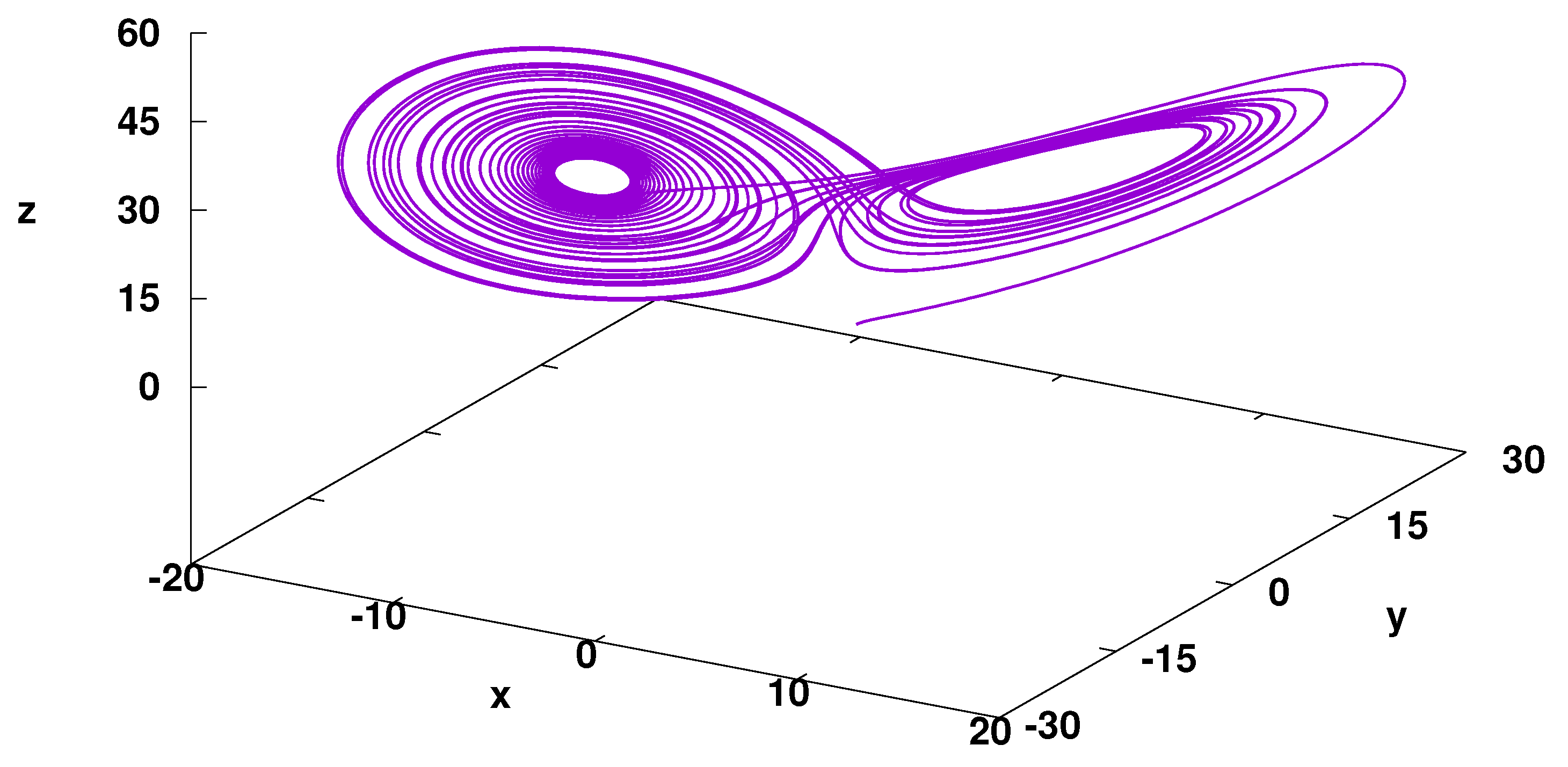
For parameter , the system shows chaotic behaviour. The example of the system evolution is presented in Figure 2. In the present study, the determinism problem of the time series is investigated for the one-dimensional system; therefore, the Lorenz Attractor system, although 3D, is analysed as one-dimensional, in which the evolution of one of the coordinates is modelled by LSTM and the quality of the model is verified.
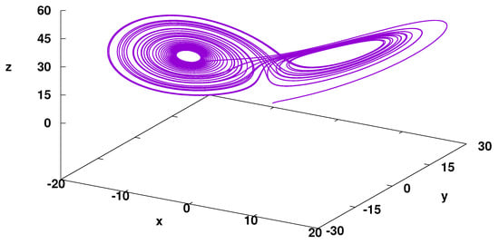
Figure 2.
Trajectory of Lorentz Attractor. Numerical solution, iterations step , iteration steps, parameters: , the initial point is (1,1,1).
3.3. Financial Time Series
The last type of data verified here is the financial time series. This is a very special type of data. In this field, despite massive effort and numerous models, e.g., [44,45,46,47], financial markets are still unpredictable. Of course, scholars cannot consider the lack of a reliable method for stock value forecasting a failure because, through theory development, we understand the stock market issue much better. However, we cannot claim that the system is deterministic. The stochastic nature of stock markets is a natural consequence of being a complex system in which human decisions play a key role.
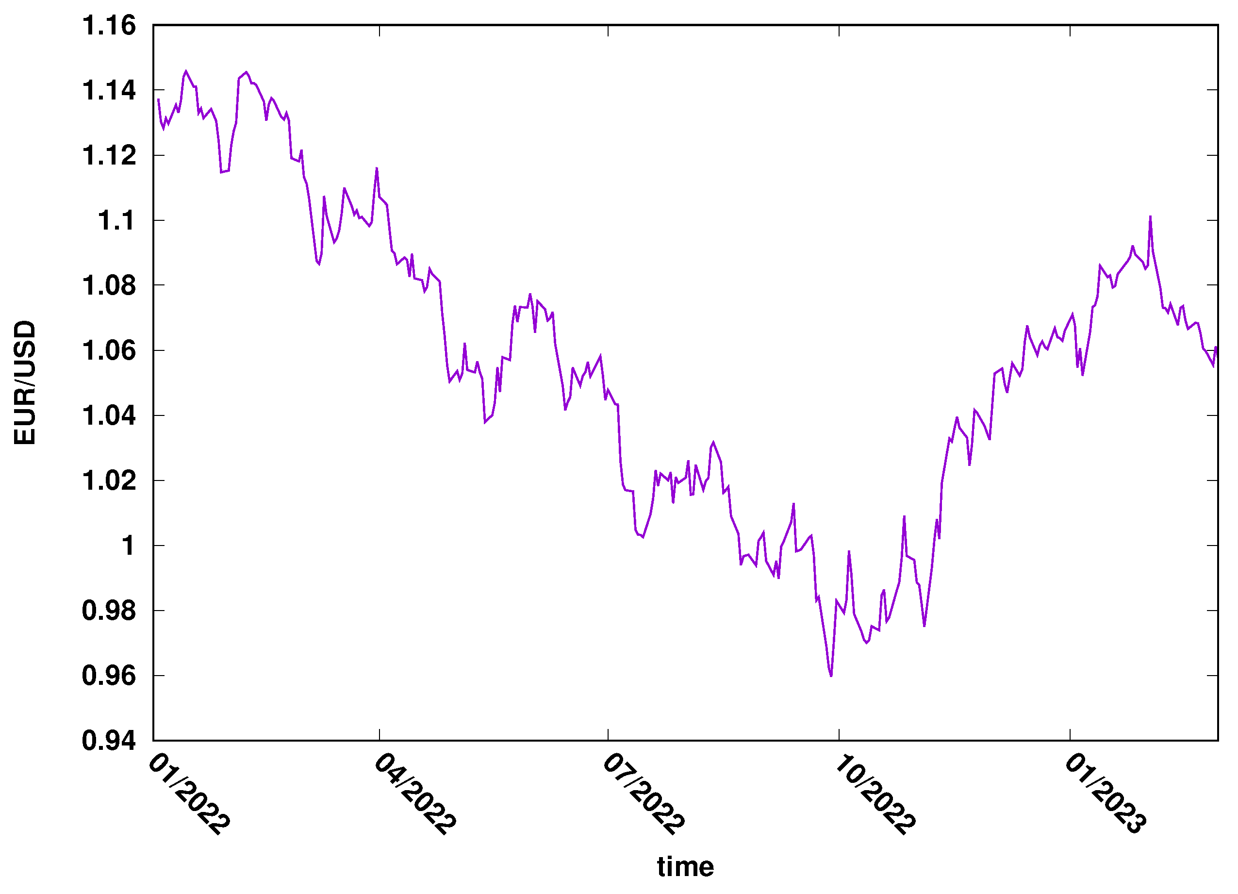
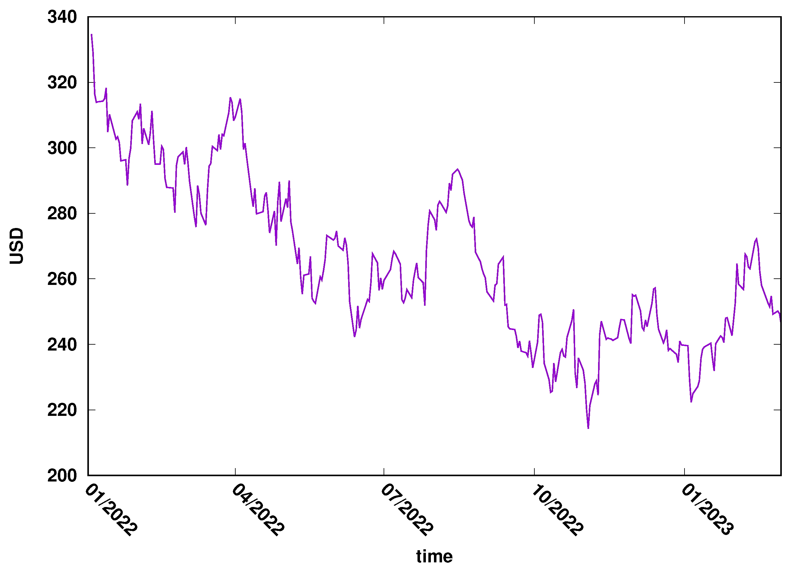
This study used two time series: the daily close exchange rate of USD/EUR (FOREX market) and Microsoft’s daily close price (MSFT) of the New York stock exchange. The most important features that determined the choice of the examples were the liquidity of those markets and their importance to the global market. The data were downloaded from the Yahoo Finance web page, covering 2022/2023. The evolution of EUR/USD is presented in Figure 3, while the evolution of MSFT daily close price can be seen in Figure 4.
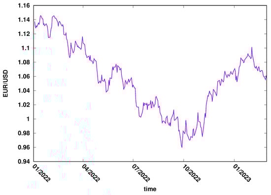
Figure 3.
The pair EUR/USD exchange rate evolution in 2022–2023. FOREX market.
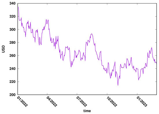
Figure 4.
The evolution of MSTF time series in 2022–2023. New York Stock Exchange.
The descriptive statistics of the analysed data are presented in Table 1. However, we do not discuss the economic background and evolution of the considered time series, as it is beyond the scope of the present study.

Table 1.
The basic statistical characteristic of the financial data.
4. LSTM Implementation (Results)
The LSTM model requires splitting the available data into three sets: training, validation, and testing. The proportion can be arbitrary, depending on the availability of the data. In the case of artificial data, the splitting is less important because the data can be easily generated. However, in the case of real data, there are significant limits due to the size of the available data. To assess the quality of trained models, the following data split pattern was used: 60% were used for training, 20% for validating the model during training, and 20% for testing the model. For all the considered time series, the same splitting pattern is used.
4.1. AR(2) Model
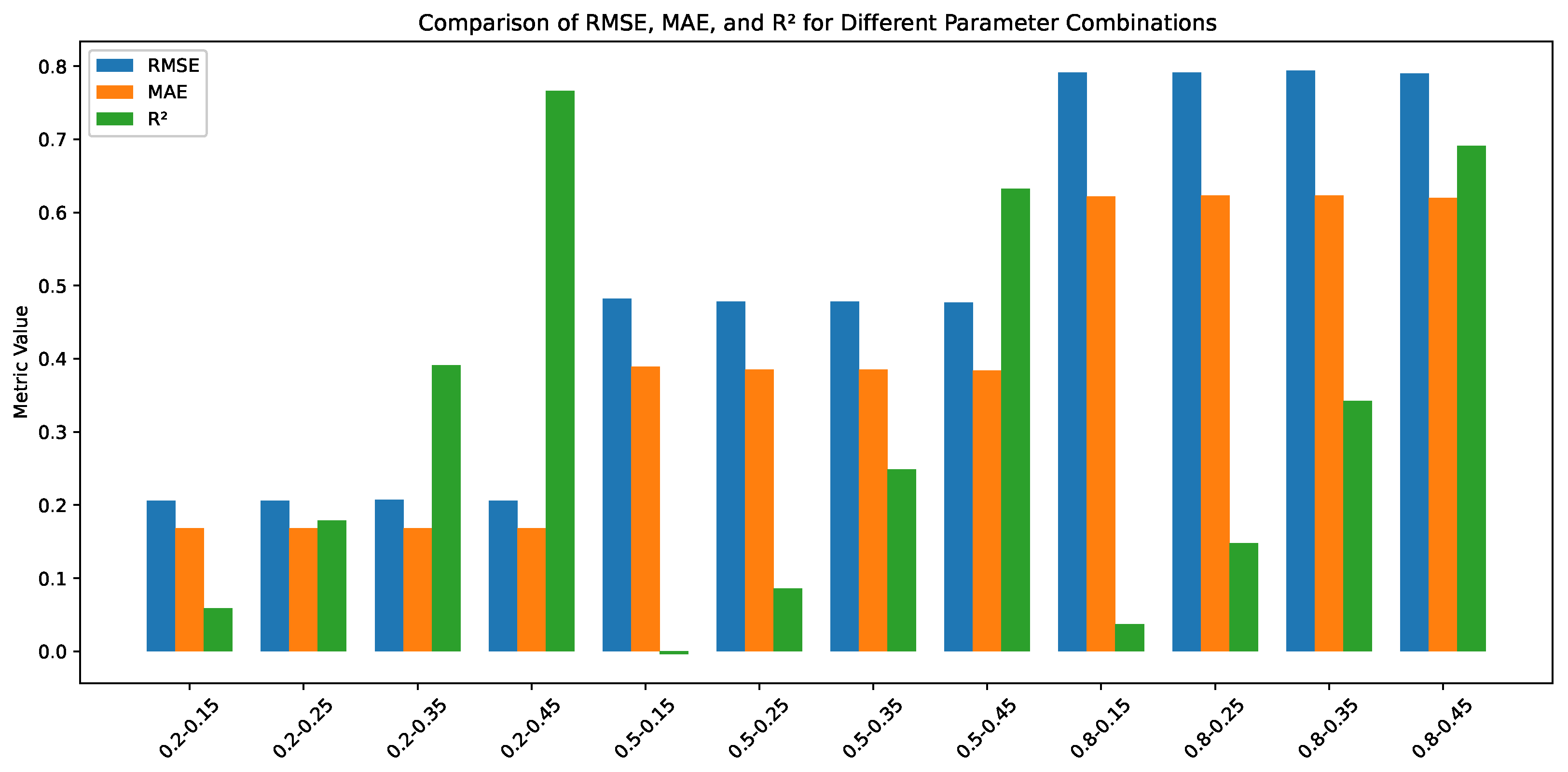
The AR(2) model allows for generating an arbitrary amount of data. However, generating extremely long time series would significantly lower the model convergence’s performance, since the time series memory is restricted to two consecutive time steps. Therefore, the time series of 5000 data points was used, the model’s training was performed on 3000 data points, and the test was conducted on 1000 data points. The main task in this part was verifying the quality of the model trained concerning the noise level in the time series. The following AR(2) models were verified: the memory coefficient and the noise standard deviation . The assumed values of the AR(2) parameters gave 12 different time series which represented a low dependence of past values and low noise up to a high dependence of the past values and high value standard deviation . It is important to notice that, due to the definition Equation (11), the past noise impulses are multiplied by the and coefficients.
The applied optimisation process of the single-layer LSTM model allows setting the models trained on AR(2) time series for different parameters. The model’s details and quality are measured as RMSE, which are presented in Table 2. For clarity, the result are also presented as Figure 5.
Table 2.
Parameter of the optimised single-layer LSTM models trained for the AR(2) time series generated for different memory coefficients and the noise level . The quality of the trained single-layer LSTM model is presented in the last column.
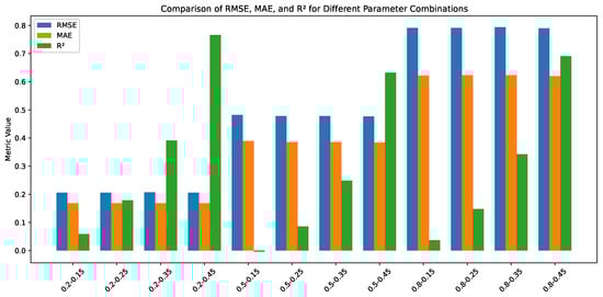
Figure 5.
Grouped bar plot comparing RMSE, MAE, and values for the AR(2) time series for different combinations of and . Each group of bars represents a unique parameter combination.
The most important observation of RMSE of the trained models in Table 2 is that the quality of the models decreases with the noise level (defined by ). It is noticeable that the AR(q) time series combines the deterministic part with the stochastic noise. Here, the value of the memory coefficient does not influence the quality of the trained models. In the case of low noise , RMSE is ≈0.21. A much higher RMSE is observed for high noise for which RMSE . Naturally, the noise disturb the possibility to recognise the determinism of the time series as it is an internal part of the time series—the consecutive time series element is calculated not only on the deterministic part but also takes into account the noise of the previous point (compared to Equation (11)). Besides the clear observation of the standard deviation influence, one can also observe that the coefficient increases as the value of the memory parameters increases. So, the quality of the trained model depends on the determinism and the randomness of the investigated time series.
4.2. Lorentz Attractor
Despite its chaotic nature, the Lorentz Attractor is a fully deterministic system, which renders it challenging to forecast. This is particularly the case due to its sensitivity to the initial conditions. However, as a theoretical problem, it is possible to generate sufficiently long time series to train and verify the quality of the model.
The model generates a trajectory in space, so it was expressed as X, Y, Z time series and used as three features for the model. For the analysis, iteration steps were generated, using a 20-point lookback length. Six thousand four hundred data points were used for training with the overlapping samples, and the model was verified on 2000 data points. Two types of LSTM networks were generated: one-layer LSTM and two-layer LSTM. And the model quality was verified in the X and Z coordinate time series. The details of optimised models and the quality of prediction are presented in Table 3 and as Figure 6. The two-layer model was used because the training of the one-layer model required significant computational time, and we decided to verify the results on the two-layer model.
Table 3.
The results of Lorentz Attractor models. The quality of the trained LSTM models is presented in the last column.
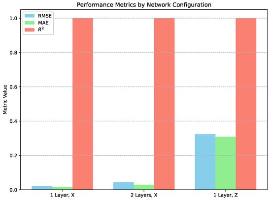
Figure 6.
Grouped bar plot comparing RMSE, MAE, and values for the Lorentz Attractor time series: one-layer and two-layer networks for X and Z coordinates.
All the fitted models have low RMSE values, even below the RMSE for AR(2) models. So, despite the chaotic and nonlinear system, the quality of the fitted model is better than that of the low-noise AR(2). Particularly interesting are the values of measures, which are practically equal one, that indicate perfect agreement between the model and the analysed data.
4.3. Financial Time Series
The main difficulty in model estimation for financial time series is the short time series. For the exchange rate of EUR/USD, the time series consists of 520 data points, while the MSFT time series has 501 data points. These values are significantly smaller than the length of the generated time series AR and Lorentz Attractor. As a consequence of the limited size of the data, the model was trained on 312 data points.
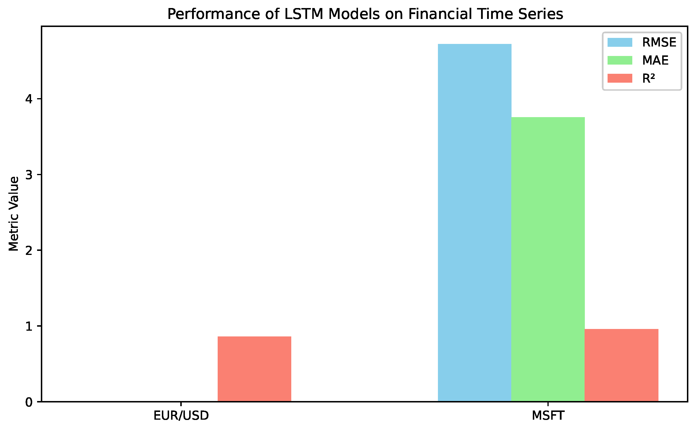
The details and quality measure of the fitted model are presented in Table 4 and in Figure 7. The quality of the LSTM model trained on the exchange rate EUR/USD is surprisingly low. However, it should be compared with the value within the time series. The range of the values observed is in the interval (0.9596, 1.1457). The difference between two consecutive data points is in the interval , and the averaged increment is 0.0045. Therefore, RMSE = 0.008 means that the relative error of prediction is approximately 150%, which is high. Analogously, the observed values for MSFT stocks are in the interval (214.25, 382.70), and the increments are in (0.01, 19.95), with an average value of 4.16. Comparing RMSE, it gives the relative error of prediction approximately 90%, so, once again, very high. It should be noticed that the trained model are characterised as relatively high values of the measures 0.860 and 0.958. One important point is that the considered time series are short (particularly comparing with the model time series), so it influences the model quality; on the other hand, the measure focuses on the variance. Indeed, the intervals for the analysis were chosen beyond the extreme event on the stock market, aside from bot time series which belongs to the highly liquid reflected in high as a result.
Table 4.
The quality of one-layer LSTM models trained on the financial time series EUR/USD and MSFT. The quality of the trained one-layer LSTM model is presented in the last column.
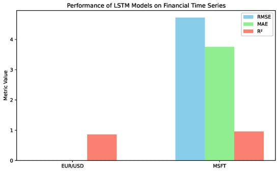
Figure 7.
Grouped bar plot comparing RMSE, MAE, and values for one-layer LSTM models trained on the EUR/USD and MSFT financial time series. RMSE and MAE for the EUR/USD exchange rate are hardly visible due to the scale of the graph.
5. Conclusions and Future Work
5.1. Key Contributions
- This study introduces a novel application of deep learning models—specifically LSTM networks—as a metric for assessing determinism in time series data.
- Unlike traditional uses of AI for prediction or classification, this research inverts the paradigm by using the model’s performance as an indicator of the underlying structure in the data.
- Theoretical insights are provided regarding the deterministic nature of AI models, emphasizing their reliance on pattern recognition and the importance of avoiding overfitting.
- The approach was empirically validated on three types of time series:
- –
- Deterministic with noise: AR(2) model—performance degraded with noise.
- –
- Deterministic: Lorenz attractor—accurately reconstructed.
- –
- Stochastic: Financial time series—poor model performance, supporting the hypothesis.
- The quality of the LSTM model, measured via RMSE, MAE, and , correlates with the degree of determinism in the time series.
5.2. Shortcomings
- The process of constructing AI models is not yet standardised, which may affect reproducibility and scalability.
- Designing optimal architectures remains a complex task, even though an optimization algorithm was employed.
- This study primarily used RMSE as the determinism indicator; however, this may not capture all aspects of model quality or data structure.
5.3. Future Prospects
- Develop a standardised pipeline for generating and validating AI models for determinism analysis.
- Develop a standardised metric for determinism analysis.
Author Contributions
Conceptualisation, J.M.; methodology, J.M.; software, P.W.; writing—original draft preparation, J.M.; writing—review and editing, J.M.; visualization, J.M.; supervision, J.M. All authors have read and agreed to the published version of the manuscript.
Funding
This research received no external funding.
Data Availability Statement
Publicly available data were used in the paper.
Conflicts of Interest
The authors declare no conflicts of interest.
References
- Ribeiro, M.; Henriques, T.; Castro, L.; Souto, A.; Antunes, L.; Costa-Santos, C.; Teixeira, A. The Entropy Universe. Entropy 2021, 23, 222. [Google Scholar] [CrossRef] [PubMed]
- Delgado-Bonal, A.; Marshak, A. Approximate Entropy and Sample Entropy: A Comprehensive Tutorial. Entropy 2019, 21, 541. [Google Scholar] [CrossRef]
- Namdari, A.; Li, Z.S. A review of entropy measures for uncertainty quantification of stochastic processes. Adv. Mech. Eng. 2019, 11, 1687814019857350. [Google Scholar] [CrossRef]
- Ausloos, M.; Miśkiewicz, J. Introducing the q-Theil index. Braz. J. Phys. 2009, 39, 388–395. [Google Scholar]
- Rotundo, G.; Ausloos, M. Complex-valued information entropy measure for networks with directed links (digraphs). Application to citations by community agents with opposite opinions. Eur. Phys. J. B 2013, 86, 169. [Google Scholar] [CrossRef]
- Bar-Hillel, M.; Wagenaar, W.A. The perception of randomness. Adv. Appl. Math. 1991, 12, 428–454. [Google Scholar] [CrossRef]
- Arcuri, A.; Iqbal, M.Z.; Briand, L. Random testing: Theoretical results and practical implications. IEEE Trans. Softw. Eng. 2011, 38, 258–277. [Google Scholar] [CrossRef]
- Sano, M.; Sawada, Y. Measurement of the Lyapunov spectrum from a chaotic time series. Phys. Rev. Lett. 1985, 55, 1082. [Google Scholar] [CrossRef] [PubMed]
- Shao, Y.H.; Gu, G.F.; Jiang, Z.Q.; Zhou, W.X.; Sornette, D. Comparing the performance of FA, DFA and DMA using different synthetic long-range correlated time series. Sci. Rep. 2012, 2, 835. [Google Scholar] [CrossRef]
- Arianos, S.; Carbone, A. Cross-correlation of long-range correlated series. J. Stat. Mech. Theory Exp. 2009, 2009, P03037. [Google Scholar] [CrossRef]
- Doukhan, P.; Oppenheim, G.; Taqqu, M. Theory and Applications of Long-Range Dependence; Springer Science & Business Media: Berlin/Heidelberg, Germany, 2002. [Google Scholar]
- Cryer, J.D. Time Series Analysis; Duxbury Press Boston: North Scituate, MA, USA, 1986; Volume 286. [Google Scholar]
- Franses, P.H. Time Series Models for Business and Economic Forecasting; Cambridge University Press: Oxford, UK, 1998. [Google Scholar]
- Wei, W.W. Time Series Analysis. In The Oxford Handbook of Quantitative Methods in Psychology: Vol. 2: Statistical Analysis; Oxford University Press: Oxford, UK, 2013. [Google Scholar] [CrossRef]
- Han, C.; Hilger, H.; Mix, E.; Böttcher, P.C.; Reyers, M.; Beck, C.; Witthaut, D.; Gorjão, L.R. Complexity and Persistence of Price Time Series of the European Electricity Spot Market. PRX Energy 2022, 1, 013002. [Google Scholar] [CrossRef]
- Chen, S.; Guo, W. Auto-encoders in deep learning—a review with new perspectives. Mathematics 2023, 11, 1777. [Google Scholar] [CrossRef]
- Zhang, Q.; Yang, L.T.; Chen, Z.; Li, P. A survey on deep learning for big data. Inf. Fusion 2018, 42, 146–157. [Google Scholar] [CrossRef]
- Yu, Y.; Si, X.; Hu, C.; Zhang, J. A review of recurrent neural networks: LSTM cells and network architectures. Neural Comput. 2019, 31, 1235–1270. [Google Scholar] [CrossRef] [PubMed]
- Shiri, F.M.; Perumal, T.; Mustapha, N.; Mohamed, R. A comprehensive overview and comparative analysis on deep learning models: CNN, RNN, LSTM, GRU. arXiv 2023, arXiv:2305.17473. [Google Scholar]
- Sherstinsky, A. Fundamentals of recurrent neural network (RNN) and long short-term memory (LSTM) network. Phys. D Nonlinear Phenom. 2020, 404, 132306. [Google Scholar] [CrossRef]
- Tsai, Y.T.; Zeng, Y.R.; Chang, Y.S. Air pollution forecasting using RNN with LSTM. In Proceedings of the 2018 IEEE 16th Intl Conf on Dependable, Autonomic and Secure Computing, 16th Intl Conf on Pervasive Intelligence and Computing, 4th Intl Conf on Big Data Intelligence and Computing and Cyber Science and Technology Congress (DASC/PiCom/DataCom/CyberSciTech), Athens, Greece, 12–15 August 2018; pp. 1074–1079. [Google Scholar]
- Abdel-Nasser, M.; Mahmoud, K. Accurate photovoltaic power forecasting models using deep LSTM-RNN. Neural Comput. Appl. 2019, 31, 2727–2740. [Google Scholar] [CrossRef]
- Hochreiter, S.; Schmidhuber, J. Long short-term memory. Neural Comput. 1997, 9, 1735–1780. [Google Scholar] [CrossRef]
- Wu, Q.; Guan, F.; Lv, C.; Huang, Y. Ultra-short-term multi-step wind power forecasting based on CNN-LSTM. IET Renew. Power Gener. 2021, 15, 1019–1029. [Google Scholar] [CrossRef]
- Koprinska, I.; Wu, D.; Wang, Z. Convolutional neural networks for energy time series forecasting. In Proceedings of the 2018 International Joint Conference on Neural networks (IJCNN), Rio de Janeiro, Brazil, 8–13 July 2018; pp. 1–8. [Google Scholar]
- Smagulova, K.; James, A.P. A survey on LSTM memristive neural network architectures and applications. Eur. Phys. J. Spec. Top. 2019, 228, 2313–2324. [Google Scholar] [CrossRef]
- Wen, X.; Li, W. Time Series Prediction Based on LSTM-Attention-LSTM Model. IEEE Access 2023, 11, 48322–48331. [Google Scholar] [CrossRef]
- Greff, K.; Srivastava, R.K.; Koutník, J.; Steunebrink, B.R.; Schmidhuber, J. LSTM: A Search Space Odyssey. IEEE Trans. Neural Netw. Learn. Syst. 2017, 28, 2222–2232. [Google Scholar] [CrossRef] [PubMed]
- Farzad, A.; Mashayekhi, H.; Hassanpour, H. A comparative performance analysis of different activation functions in LSTM networks for classification. Neural Comput. Appl. 2019, 31, 2507–2521. [Google Scholar] [CrossRef]
- Vijayaprabakaran, K.; Sathiyamurthy, K. Towards activation function search for long short-term model network: A differential evolution based approach. J. King Saud Univ.-Comput. Inf. Sci. 2022, 34, 2637–2650. [Google Scholar] [CrossRef]
- Duchi, J.; Hazan, E.; Singer, Y. Adaptive Subgradient Methods for Online Learning and Stochastic Optimization. J. Mach. Learn. Res. 2011, 12, 2121–2159. [Google Scholar]
- Ruder, S. An overview of gradient descent optimization algorithms. arXiv 2017, arXiv:1609.04747. [Google Scholar]
- Alamri, N.M.H.; Packianather, M.; Bigot, S. Optimizing the Parameters of Long Short-Term Memory Networks Using the Bees Algorithm. Appl. Sci. 2023, 13, 2536. [Google Scholar] [CrossRef]
- Nwankpa, C.; Ijomah, W.; Gachagan, A.; Marshall, S. Activation functions: Comparison of trends in practice and research for deep learning. arXiv 2018, arXiv:1811.03378. [Google Scholar]
- Dubey, S.R.; Singh, S.K.; Chaudhuri, B.B. Activation functions in deep learning: A comprehensive survey and benchmark. Neurocomputing 2022, 503, 92–108. [Google Scholar] [CrossRef]
- Bai, Y. RELU-function and derived function review. In Proceedings of the SHS Web of Conferences, Kunming, China, 23–25 December 2022; EDP Sciences: Les Ulis, France, 2022; Volume 144, p. 02006. [Google Scholar]
- Available online: https://optuna.org/ (accessed on 10 November 2024).
- Lütkepohl, H.; Krätzig, M. Applied Time Series Econometrics; Cambridge University Press: Cambridge, UK, 2004. [Google Scholar]
- Tsay, R.S. Analysis of Financial Time Series; John Wiley & Sons: Hoboken, NJ, USA, 2005. [Google Scholar]
- Schuster, H.G.; Just, W. Deterministic Chaos: An Introduction; John Wiley & Sons: Hoboken, NJ, USA, 2005. [Google Scholar] [CrossRef]
- Lorenz, E.N. Deterministic Nonperiodic Flow. J. Atmos. Sci. 1963, 20, 130–141. [Google Scholar] [CrossRef]
- Viswanath, D. The fractal property of the Lorenz attractor. Phys. D Nonlinear Phenom. 2004, 190, 115–128. [Google Scholar] [CrossRef]
- Guckenheimer, J.; Williams, R.F. Structural stability of Lorenz attractors. Publ. Mathématiques L’IHÉS 1979, 50, 59–72. [Google Scholar] [CrossRef]
- Poon, S.H.; Granger, C.W.J. Forecasting volatility in financial markets: A review. J. Econ. Lit. 2003, 41, 478–539. [Google Scholar] [CrossRef]
- Cavalcante, R.C.; Brasileiro, R.C.; Souza, V.L.; Nobrega, J.P.; Oliveira, A.L. Computational intelligence and financial markets: A survey and future directions. Expert Syst. Appl. 2016, 55, 194–211. [Google Scholar] [CrossRef]
- Milana, C.; Ashta, A. Artificial intelligence techniques in finance and financial markets: A survey of the literature. Strateg. Chang. 2021, 30, 189–209. [Google Scholar] [CrossRef]
- Samanidou, E.; Zschischang, E.; Stauffer, D.; Lux, T. Agent-based models of financial markets. Rep. Prog. Phys. 2007, 70, 409. [Google Scholar] [CrossRef]

Disclaimer/Publisher’s Note: The statements, opinions and data contained in all publications are solely those of the individual author(s) and contributor(s) and not of MDPI and/or the editor(s). MDPI and/or the editor(s) disclaim responsibility for any injury to people or property resulting from any ideas, methods, instructions or products referred to in the content. |
© 2025 by the authors. Licensee MDPI, Basel, Switzerland. This article is an open access article distributed under the terms and conditions of the Creative Commons Attribution (CC BY) license (https://creativecommons.org/licenses/by/4.0/).