ED-SA-ConvLSTM: A Novel Spatiotemporal Prediction Model and Its Application in Ionospheric TEC Prediction

Abstract

The ionospheric total electron content (TEC) has complex spatiotemporal variations, making its spatiotemporal prediction challenging. Capturing long-range spatial dependencies is of great significance for improving the spatiotemporal prediction accuracy of TEC. Existing work based on Convolutional Long Short-Term Memory (ConvLSTM) primarily relies on convolutional operations for spatial feature extraction, which are effective at capturing local spatial correlations, but struggle to model long-range dependencies, limiting their predictive performance. Self-Attention Convolutional Long Short-Term Memory (SA-ConvLSTM) can selectively store and focus on long-range spatial dependencies, but it requires the input length and output length to be the same due to its “n vs. n” structure, limiting its application. To solve this problem, this paper proposes an encoder-decoder SA-ConvLSTM, abbreviated as ED-SA-ConvLSTM. It can effectively capture long-range spatial dependencies using SA-ConvLSTM and achieve unequal input-output lengths through encoder–decoder structure. To verify its performance, the proposed ED-SA-ConvLSTM was compared with C1PG, ConvLSTM, and PredRNN from multiple perspectives in the area of 12.5° S–87.5° N, 25° E–180° E, including overall quantitative comparison, comparison across different months, comparison at different latitude regions, visual comparisons, and comparison under extreme situations. The results have shown that, in the vast majority of cases, the proposed ED-SA-ConvLSTM outperforms the comparative models.

1. Introduction

The ionosphere is the upper layer of the atmosphere that is ionized via high-energy solar radiation and cosmic rays. It contains a large number of charged particles. When Global Positioning System (GPS) signals pass through the ionosphere, the path of the signal bends and the propagation speed changes, resulting in a deviation in the measured distance, causing an ionospheric delay [1]. Ionospheric delay is the main source of error in Global Navigation Satellite System (GNSS) based applications [2]. The ionosphere total electron content (TEC), which is a parameter describing the state of the ionosphere, is used to calculate ionospheric delay. Thus, TEC prediction is of great significance for correcting ionospheric delay and improving the accuracy of the GNSS based applications.

TEC is influenced by various factors, such as solar activity, local time, and geomagnetic storms, exhibiting highly complex and nonlinear variations. As a result, TEC prediction is very challenging [3]. Recently, deep learning models have gained significant success in a variety of fields due to their excellent nonlinear representation ability [4,5,6]. Deep learning technology has also dominated the field of TEC prediction, and developing high-precision deep learning models has become a hot topic in TEC prediction. Compared to traditional ionospheric empirical models, such as the International Reference Ionosphere (IRI) model [7], Bent model [8], NeQuick model [9,10], and statistical models such as the autoregressive moving average(ARMA) [11,12], autoregressive integrated moving average(ARIMA) [13], deep learning models have demonstrated superiority in TEC prediction [14,15,16].

Deep learning models for TEC prediction can be roughly classified into two categories:(1) Time series models. These models in this category consider TEC prediction as a time series problem. They usually model TEC historical sequences from a single location to generate the output TEC sequences at that same location. The most commonly used models in this type are unidirectional time series models, such as LSTM [17,18], GRU [19], and ED-LSTME [20]. Then, bidirectional time series models, such as BiLSTM [21,22,23], were introduced for TEC prediction, which have been proven to have stronger nonlinear representation capabilities than unidirectional ones. Later, researchers combined convolutional neural networks (CNN) with time series models to model both the temporal and local positional patterns of TEC sequences. The combination models include CNN-LSTM [24], CNN-GRU [25], and CNN-BiLSTM [26]. Recently, attention mechanisms have been embedded into TEC time series models due to their capability to focus on important features and suppress unimportant ones. Then, embedding attention mechanisms in deep learning models has become a research hotspot in TEC prediction, such as Attentional BiGRU [27], Attention BiLSTM [28], and Att-CNN-BiLSTM [29]. Although time series models have made some progress in TEC prediction, their performance still needs to be improved as they ignore spatial features, such as the correlations between TECs in adjacent regions. (2) Spatiotemporal models. Models in this category receive TEC map sequences as input, then extract temporal and spatial features from them, and generate the predicted future TEC maps. The most famous spatiotemporal model is ConvLSTM, which was originally used for precipitation prediction [30], and then has been introduced for TEC prediction [31,32]. Afterwards, various variants of ConvLSTM emerged in TEC prediction, such as Attention ConvLSTM [33], ED-ConvLSTM [34,35,36], ED-AttConvLSTM [37], ConvGRU [38], BiConvLSTM [1,39], and BiConvGRU [40].

Spatiotemporal models, such as ConvLSTM and its variants, are dominant in TEC prediction. However, they also have some flaws. In TEC prediction, the key issue is to model the complex dynamic long-range spatial dependencies in TEC map sequences. When generating TEC prediction maps, long-range spatial dependence refers to the periodic variation pattern between TEC maps at time steps that are farther away from the predicted time. TEC map exhibits multi-scale temporal variations: in the short term, TEC maps are highly correlated with their adjacent time steps due to continuity of data; in the medium to long term, it exhibits annual periodic changes due to influence of the Earth’s revolution; and influenced by the solar activity cycle, the TEC map shows periodic changes of about 11 years. For TEC map prediction, the longer the spatiotemporal dependency span of memory, the more knowledge can be learned from historical data, resulting in better prediction performance. In those ConvLSTM-based models, spatial features are extracted using convolution, which can effectively capture local dependencies. To capture long-range dependencies, stacking multiple convolutional layers is necessary. This approach can result in an effective receptive field that is much smaller than the theoretical receptive field, diminishing the efficiency of capturing long-range dependencies [41]. As a solution, Wang et al. proposed a new spatiotemporal model called PredRNN in 2017, which adds a spatial memory to ConvLSTM to store long-range spatial memory [42]. However, in PredRNN, the long-range spatial memory has not been selectively focused and suppressed, and there is still room for improvement. Inspired by self-attention, Lin et al. proposed the Self-Attention Memory (SAM) module to focus and suppress long-range spatial memory, then embedded it into ConvLSTM, and proposed SA-ConvLSTM [43]. SA-ConvLSTM uses self-attention to strengthen and suppress long-range spatial memory and aggregates it with short-distance memory. In this way, it solves the problem of ConvLSTM being unable to effectively extract long-range spatial dependencies and PredRNN being unable to focus and suppress long-range spatial memory.

SA-ConvLSTM can selectively store and focus on long-range and short-distance spatial dependencies, which is superior to ConvLSTM in some applications of deep learning. This paper introduced it for TEC spatiotemporal prediction. The original SA-ConvLSTM adopts an “n vs. n” structure. This structure requires the input length and output length of the model to be the same, which limits the application of SA-ConvLSTM. To solve this problem, this paper redesigns SA-ConvLSTM using an encoder–decoder structure and proposes the encoder–decoder SA-ConvLSTM, abbreviated as ED-SA-ConvLSTM. This paper is the first to redesign SA-ConvLSTM using an encoder–decoder structure, making it suitable for more spatiotemporal prediction tasks. The proposed ED-SA-ConvLSTM is divided into two parts: the encoder part receives the TEC map sequence and converts it into a final spatiotemporal feature map; the decoder part decodes the final spatiotemporal feature map and converts it into the predicted TEC map sequence. This improvement allows for different input and output lengths of the model, making it more flexible. In addition, existing research has shown that the encoder–decoder structure is superior to the “n vs. n” structure [44,45,46].

To validate the performance of the proposed ED-SA-ConvLSTM, we selected the 12.5° S–87.5° N, 25° E–180° E regions as the study area. Within this area, a 6-year TEC map sequence was selected as the dataset, including 3 years of high solar activity and 3 years of low solar activity. On this dataset, the proposed ED-SA-ConvLSTM was compared against ConvLSTM, PredRNN, and C1PG from multiple perspectives. Among these three comparative models, ConvLSTM and PredRNN are the state-of-the-art spatiotemporal prediction models. C1PG is a one-day TEC prediction product provided by the Center for Orbit Determination in Europe (CODE), which can be considered a benchmark for TEC prediction. Experimental results show that in the vast majority of cases, the predictive performance of the proposed ED-SA-ConvLSTM is better than those of the comparative models.

2. Data and Data Processing

In this paper, the TEC maps used are Global Ionospheric Map (GIM) data provided by the International GNSS Service (IGS). These TEC maps have a longitude resolution of 5°, a latitude resolution of 2.5°, and a time resolution of 2 h. To reduce computational complexity, this paper focuses on the Asia area (25° E–180° E, 12.5° S–87.5° N).

For the convenience of comparison under different solar activities, the TEC dataset includes TEC maps from 3 years of high solar activity (2013–2015) and 3 years of low solar activity (2017–2019). Among them, 4 years are used as the training set (2013, 2014, 2017, and 2018), while the rest 2 years are used as the test set (2015 and 2019). A sliding window method is used to divide samples, with the window slides for one day at a time. Subsequent experiments show that the model has the best performance when the input length is 2 days and the output length is 1 day. The specific partitioning process is shown in Figure 1, in which each box represents 12 TEC maps for a day.

To prevent the model from being biased by large data, we normalize the dataset using the Min–Max standardization method, which is calculated as follows:

$$X^{\prime }={\displaystyle \frac{X-X_{min}}{X_{max}-X_{min}}},$$

(1)

where $X$ denotes the original TEC map, $X^{\prime }$ is the standardized TEC map, and $X_{min}$ and $X_{max}$ represent the minimum and maximum of $X$ in the training set, respectively.

3. Methodology

The proposed ED-SA-ConvLSTM adopts an encoder–decoder structure to organize SA-ConvLSTM units. Therefore, this section first introduces the SA-ConvLSTM unit, then the proposed ED-SA-ConvLSTM.

3.1. SA-ConvLSTM

The self-Attention Convolutional Long Short-Term Memory (SA-ConvLSTM) can be seen as a variant of ConvLSTM by extending the standard ConvLSTM architecture through integration of a Self-Attention Memory (SAM) module. This subsection will present SAM and SA-ConvLSTM.

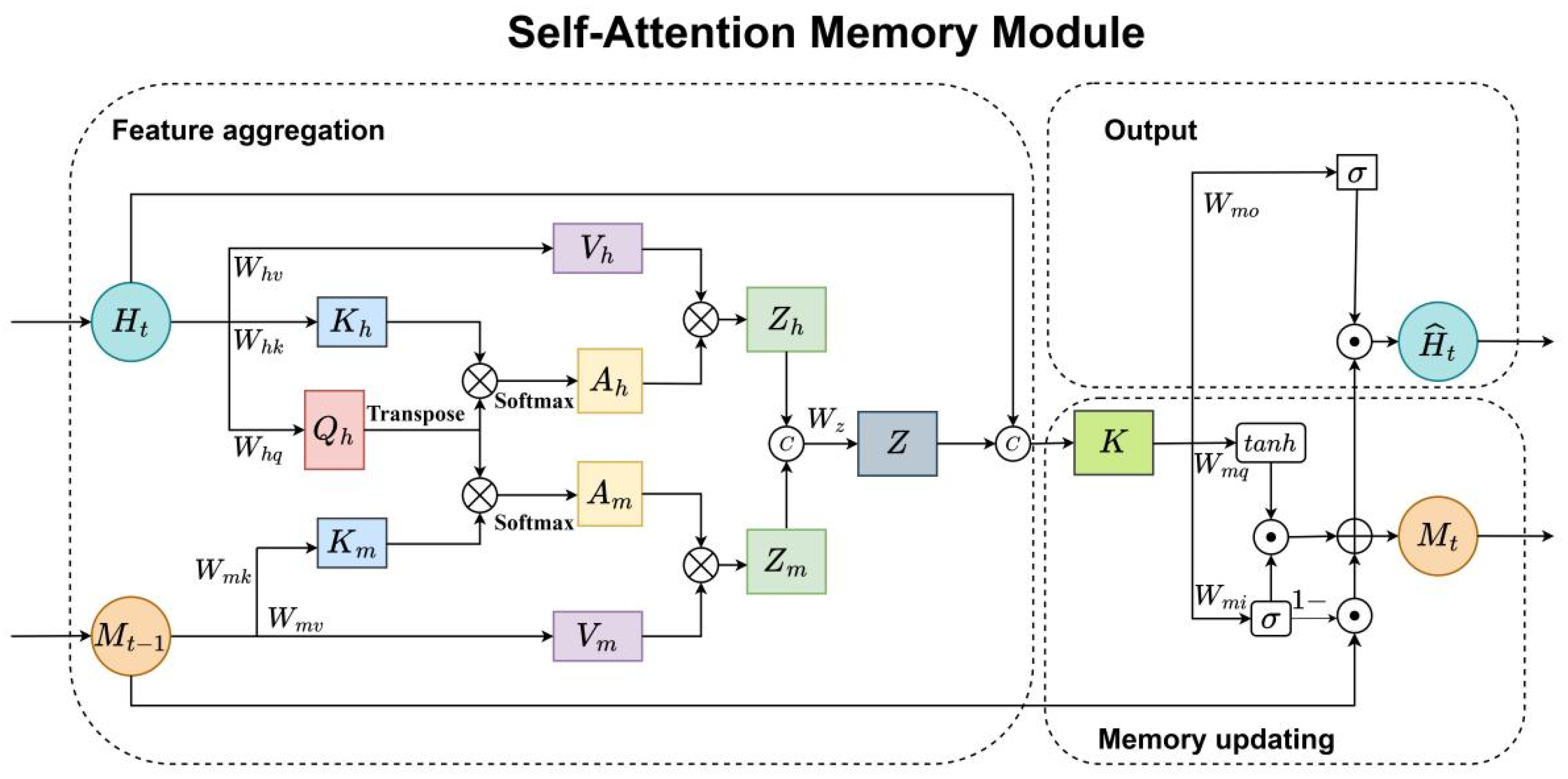
3.1.1. Self-Attention Memory (SAM) Module

The structure of the SAM is shown in Figure 2, where $M_t$ is the current memory state saves long-range spatial dependencies.

SAM contains two inputs, namely $H_t$ as the current time step and $M_{t-1}$ as the previous time step. It consists of three parts: feature aggregation, memory updating, and output generation.

●

Feature aggregation: This part first weights to the features of the current time step $Z_h$. It obtained by applying self-attention to $H_t$. And the long-range spatial memory features $Z_m$ is calculated using $V_m$ and similarity score $A_m$. Finally, $Z_h$ and $Z_m$ are aggregated into $Z$. The calculation of weighted features $Z_h$ and $Z_m$ are shown in Equations (2) and (3), respectively.

$$\left\{\begin{array}{c}{Q}_h=W_{hq}{H}_t;K_h=W_{hk}{H}_t;V_h=W_{hv}{H}_t\\ A_h=softmax\left(Q_h^T{K}_h\right)\\ Z_h=A_h{V}_h\end{array}\right.$$

(2)

$$\left\{\begin{array}{c}{Q}_h=W_{hq}{H}_t;K_m=W_{mk}{M}_{t-1};V_m=W_{mv}{M}_{t-1}\\ A_m=softmax\left(Q_h^T{K}_m\right)\\ Z_m=A_m{V}_m\end{array}\right.$$

(3)

The weighted current feature $Z_h$ and the weighted long-range memory state $Z_m$ are connected to obtain the aggregated feature $Z$. The calculation is as follows:

$$Z=W_Z\left[Z_h;Z_m\right].$$

(4)

In Equations (2)–(4), $H_t$ is the hidden layer feature at the current time step, $M_{t-1}$ is the long-range spatial memory from the previous step, $W_{hq}$, $W_{hk}$, $W_{hv}$, $W_{mk}$, and $W_{mv}$, $W_z$ are weight matrices, while $Q_h$, $K_h$, $K_m$, $V_h$, and $V_m$ are the intermediate vectors that help to calculate the attention scores of $H_t$ and $M_{t-1}$, and $\left[;\right]$ denotes vector concatenation.

●

Memory updating: The function of memory updating is to update the long-range spatial memory $M_t$ adaptively. The aggregated $Z$ and the hidden layer feature of the current time step $H_t$ are connected to form $K$. The calculations are shown in Equation (5):

$$\left\{\begin{array}{c}K=\left[H_t;Z\right]\\ i_t^{\prime }=\sigma \left(W_{mi}\ast K+b_{mi}\right)\\ g_t^{\prime }=tanh\left(W_{mg}\ast K+b_{mg}\right)\\ M_t=\left(1-i_t^{\prime }\right)⨀M_{t-1}+i_t^{\prime }⨀g_t^{\prime }\end{array}\right.,$$

(5)

where * denotes convolution, and ⨀ represents the Hadamard product.

●

Output: The output part ultimately generates a new $H_t$ using a dot product between the output gate $o_t^{\prime }$ and update memory $M_t$. Its calculation is as follows:

$$\left\{\begin{array}{c}{o}_t^{\prime }=\sigma \left(W_{mo}\ast K+b_{mo}\right)\\ {\widehat{H}}_t=o_t^{\prime }⨀M_t\end{array}\right..$$

(6)

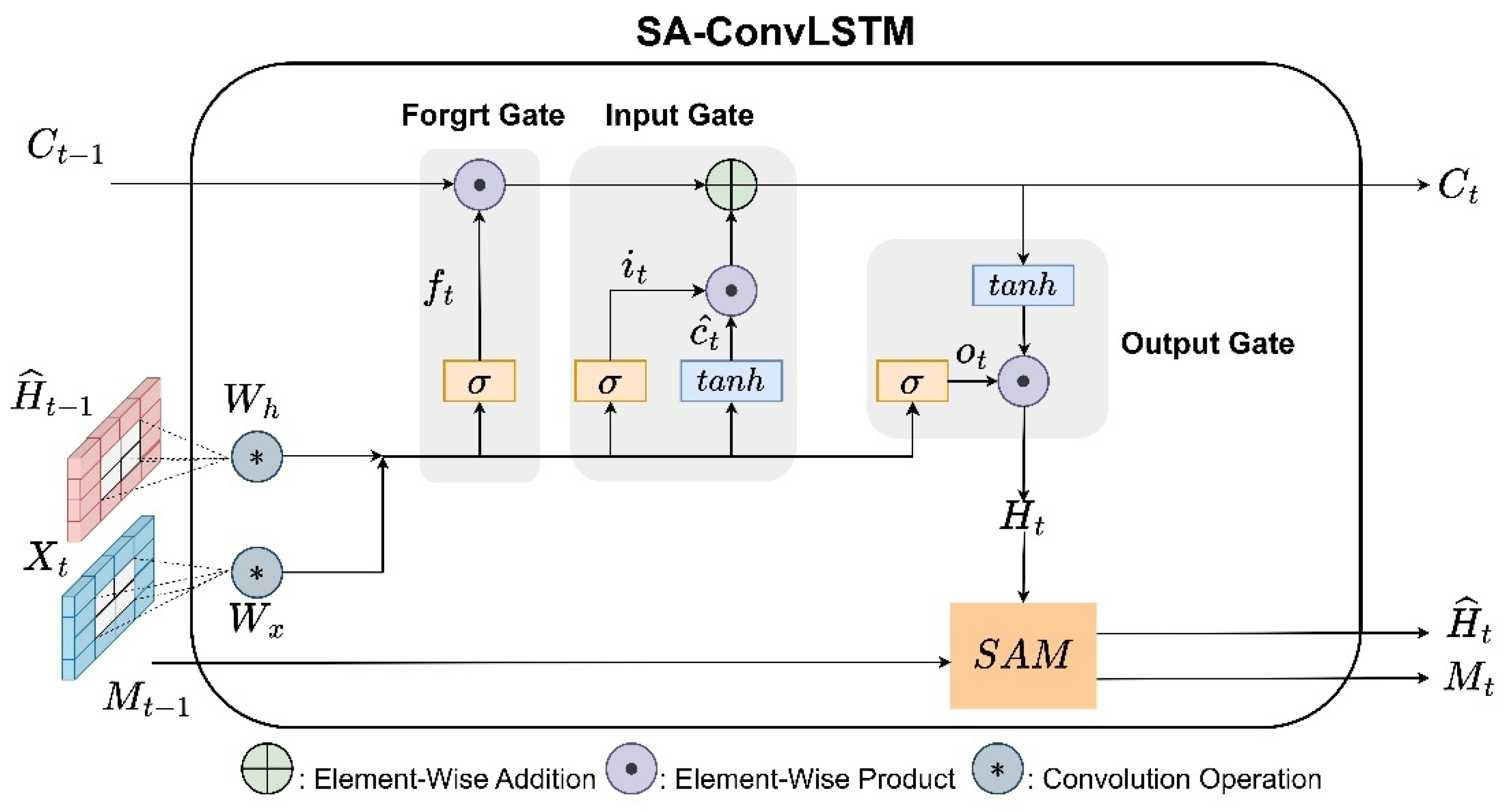
3.1.2. SA-ConvLSTM Unit

SAM module is embedded in ConvLSTM to form SA-ConvLSTM. The structure of an SA-ConvLSTM unit is shown in Figure 3. It includes three gates (the forget gate $f_t$, the input gate $i_t$, and the output gate $o_t$) and the SAM module. The calculations are shown in Equation (7):

$$\left\{\begin{array}{c}{f}_t=\sigma \left(W_f\ast \left[X_t{,\widehat{H}}_{t-1}\right]+b_f\right)\\ i_t=\sigma \left(W_i\ast \left[X_t{,\widehat{H}}_{t-1}\right]+b_i\right)\\ {\widehat{c}}_t=tanh\left(W_c\ast \left[X_t{,\widehat{H}}_{t-1}\right]+b_c\right)\\ o_t=\sigma \left(W_o\ast \left[X_t{,\widehat{H}}_{t-1}\right]+b_o\right)\\ C_t=f_t\odot C_{t-1}+i_t\odot {\widehat{c}}_t\\ H_t=o_t\odot tanh\left(C_t\right)\end{array}\right..$$

(7)

Among them, $X_t$ is the current input, $H_t$ is the current feature extracted using ConvLSTM, and ${\widehat{H}}_{t-1}$ is the output from the previous time step.

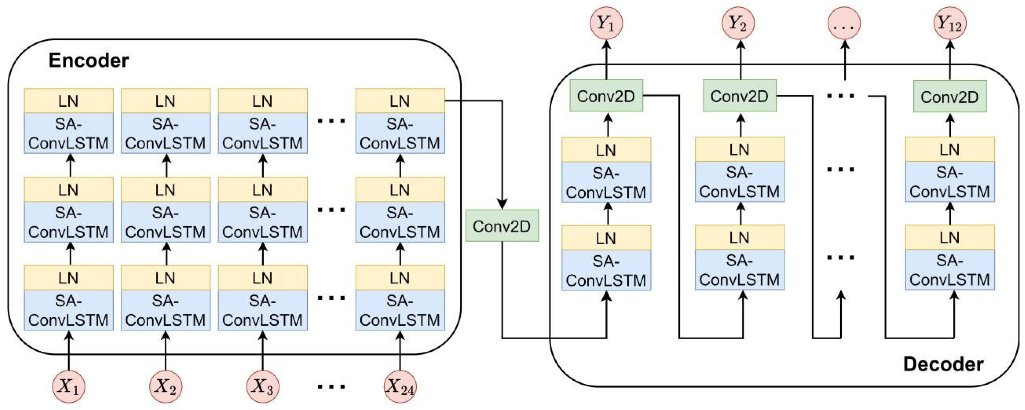
3.2. The Proposed ED-SA-ConvLSTM

The previous subsection introduced the basic structure of the SA-ConvLSTM unit. In this subsection, a novel TEC spatiotemporal prediction model was built using SA-ConvLSTM as the basic blocks.

In the original SA-ConvLSTM model, which uses the “n vs. n” structure, data flows through its layers in a “sequence-sequence” manner. This means that any layer in the network receives a sequence of length n and outputs a sequence of the same length. The model with “n vs. n” structure cannot be applied to variable-length prediction. This paper proposes a model, ED-SA-ConvLSTM, by redesigning SA-ConvLSTM using an encoder–decoder structure. The structure of ED-SA-ConvLSTM is shown in Figure 4, which consists of two parts: the encoder part and the decoder part.

The encoder part receives TEC map sequences as input, extracting spatiotemporal features from them and ultimately transforming these spatiotemporal features into a final spatiotemporal feature map. Subsequent experiments in this paper indicate that to predict the TEC maps for the next day, an input length of two days is optimal. So, the tensor size accepted for the encoder part is (24, 40, 32, and 1), with “24” indicating the input length (12 TEC maps from 2 days are used as input), “1” representing the singular feature channel, “40” and “32” being the grid size of each TEC map. In the encoder, three SA-ConvLSTM layers are used to extract features from the input spatiotemporal feature map. To prevent data from changing at each layer, which leads to gradient vanishing or explosion, we added a Layer Normalization (LN) layer after each SA-ConvLSTM layer to standardize the data. Finally, a Conv2D layer is used to aggregate the sequence of spatiotemporal feature maps and transform them into a single final spatiotemporal feature map.

The decoder part receives the final spatiotemporal feature map generated using the encoder and decodes it through two pairs of cascaded SA-ConvLSTM and LN layers. The decoder adopts a stepwise recursive prediction method: first, it generates the TEC prediction map at the current time, and then uses the current prediction map as the input to generate the prediction for the next time step. By continuously repeating this process, the decoder ultimately generates 12 TEC maps through this step-by-step prediction method. The stepwise recursive prediction method is a conventional approach to solve multi-step prediction using recursive neural networks [47].

Obviously, from the above description, in the proposed ED-SA-ConvLSTM, the flow of data is “sequence-feature-sequence”. Namely, the model receives a certain length TEC map sequence, converts it into fixed TEC spatiotemporal features using the encoder, then decodes it through the decoder, and finally generates variable lengths TEC sequence. The data flow pattern of “sequence-feature-sequence” in the encoder–decoder structure can adapt to variable length prediction problems, which overcomes the shortcomings of the original SA-ConvLSTM.

3.3. Evaluation Metrics

To evaluate the performance of the proposed model and the comparative models, this paper uses two evaluation metrics: Root Mean Square Error ($RMSE$) and Mean Absolute Percentage Error ($MAPE$), which are as follows:

$$RMSE=\sqrt{{\displaystyle \frac{1}{n}}\sum _{i=1}^n{\left(y_i-{\widehat{y}}_i\right)}^2}$$

(8)

$$MAPE={\displaystyle \frac{1}{n}}\sum _{i=1}^n\left|{\displaystyle \frac{y_i-{\widehat{y}}_i}{y_i}}\right|\times 100\%$$

(9)

Among them, n is the number of samples in the test set; $y_i$ and ${\widehat{y}}_i$ denote the true and predicted values, respectively.

4. Experimental Results

All deep learning models in this paper are built using PyTorch 1.11.0. For all the deep learning models, the optimizer is Adaptive Motion Estimation (ADAM); the loss function is Mean Square Error (MSE); the learning rate is dynamically adjusted using the CosineAnnealingWarmRestarts strategy, with an initial value of 0.001 and adjusted every 50 iterations; the maximum number of iterations is 300.

4.1. Model Optimization

C1PG is a prediction product provided by CODE, which needs no optimization, while ED-SA-ConvLSTM, ConvLSTM, and PredRNN are deep learning models. And there are many hyperparameters that will affect their performance. These three models need to be optimized. In this paper, we use Bayesian optimization to optimize the two most important hyperparameters of these three models: the number and size of convolution kernels (represented Filter and Kernel size separately). The optimization results via Bayesian optimization are shown in

Table 1. Best hyperparameters found via Bayesian optimization.

Model	Hyperparameter Setting
	Filter	Kernel Size
ConvLSTM	64	5
PredRNN	13	5
ED-SA-ConvLSTM	16	3

. In the subsequent experiments, the hyperparameters of ED-SA-ConvLSTM, ConvLSTM, and PredRNN were set to the values in Table 1.

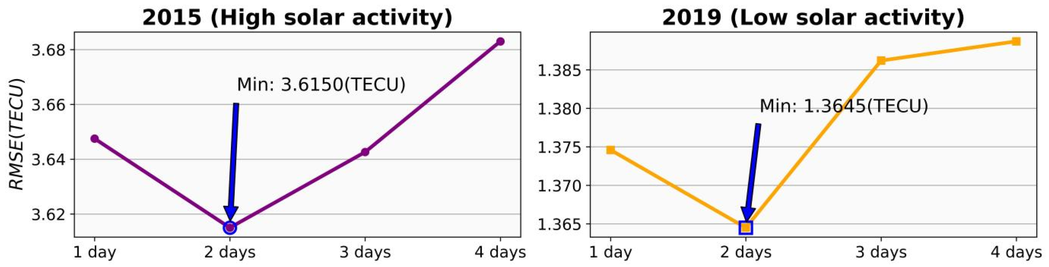
4.2. The Input Length

This subsection discusses the input length required to predict the TEC maps for the next day. Figure 5 shows the predictive performance of the model when the input length is 1 to 4 days, where the left side represents the $RMSEs$ for 2015 (a period of high solar activity), and the right demonstrates the $RMSEs$ for 2019 (a period of low solar activity).

Obviously, whether during high or low solar activity years, it is best when the input length is 2 days. So, in subsequent experiments, an input length of each deep learning model is 2 days (including 24 TEC maps), and an output length is 1 day (12 TEC maps).

4.3. Ablation Experiment

In this subsection, we first verify the effectiveness of the encoder–decoder structure through an ablation experiment. In the original SA-ConvLSTM, variable-length prediction cannot be directly achieved. Therefore, we added Conv3D at the end of the original SA-ConvLSTM to adjust the output length to one day.

The results of the ablation experiment are shown in

Table 2. The results of the ablation experiment.

Solar Activity	Model	$\mathit{R}\mathit{M}\mathit{S}\mathit{E}\left(\mathit{T}\mathit{E}\mathit{C}\mathit{U}\right)$	$\mathit{M}\mathit{A}\mathit{P}\mathit{E}$
High solar activity (2015)	SA-ConvLSTM	3.6977	13.12%
	ED-SA-ConvLSTM	3.6150	12.82%
Low solar activity (2019)	SA-ConvLSTM	1.4003	14.36%
	ED-SA-ConvLSTM	1.3645	12.93%

, in which the $RMSE$ of ED-SA-ConvLSTM decreased by 2.24% and 2.56% compared to those of SA-ConvLSTM under high solar activity and low solar activity, respectively. From the perspective of $MAPE$, ED-SA-ConvLSTM outperforms SA-ConvLSTM in both solar activities. These prove the superiority of the encoder–decoder structure over “n vs. n” structure.

4.4. Comparison with Other Models

In this part, ED-SA-ConvLSTM was compared with C1PG, ConvLSTM, and PredRNN from multiple perspectives. Each model receives TEC map sequences from two days, processes them through an encoder–decoder structure, and finally generates TEC map sequences for the next day.

4.4.1. Overall Quantitative Comparison

This subsection provides an overall quantitative comparison on the test set.

Table 3. Overall comparison on test set (The best is bolded).

Solar Activity	Model	$\mathit{R}\mathit{M}\mathit{S}\mathit{E}\left(\mathit{T}\mathit{E}\mathit{C}\mathit{U}\right)$	$\mathit{M}\mathit{A}\mathit{P}\mathit{E}$
High solar activity (2015)	C1PG	4.0295	16.12%
	ConvLSTM	3.8936	14.47%
	PredRNN	3.7928	13.95%
	ED-SA-ConvLSTM	3.6150	12.82%
Low solar activity (2019)	C1PG	1.5421	14.95%
	ConvLSTM	1.4222	14.01%
	PredRNN	1.4031	13.89%
	ED-SA-ConvLSTM	1.3645	12.93%

shows the overall quantitative comparison results of ED-SA-ConvLSTM model and three comparative models during high and low solar activity. Apparently, compared to C1PG, ConvLSTM, and PredRNN, the $RMSE$ of the proposed ED-SA-ConvLSTM decreased by 10.27%, 7.16%, and 4.53% in 2015 (high solar activity), and by 11.46%, 4.06%, and 2.75% in 2019 (low solar activity). In addition, the $MAPEs$ of ED-SA-ConvLSTM is significantly lower than those of the comparative models under both solar activities, demonstrating the effectiveness of the proposed ED-SA-ConvLSTM.

Furthermore, for a more detailed quantitative comparison, we first calculated the absolute error $\left|∆\right|$($\left|∆\right|=\left|y^{predict}-y^{true}\right|$) of each model at every grid point on each map in the test set. Then, under different solar activities, the absolute error is subdivided into several small intervals. Finally, the percentage of each model within each error interval is counted, and the results are shown in

Table 4. Absolute error distribution statistics for 2015 (The best is bolded).

Model	$\left|∆\right|\le 0.5\mathit{T}\mathit{E}\mathit{C}\mathit{U}$	$\left|∆\right|\le 1\mathit{T}\mathit{E}\mathit{C}\mathit{U}$	$\left|∆\right|\le 1.5\mathit{T}\mathit{E}\mathit{C}\mathit{U}$	$\left|∆\right|\le 2\mathit{T}\mathit{E}\mathit{C}\mathit{U}$	$\left|∆\right|\le 2.5\mathit{T}\mathit{E}\mathit{C}\mathit{U}$
C1PG	15.58%	28.85%	40.75%	51.00%	59.65%
ConvLSTM	16.51%	31.66%	44.67%	55.38%	63.88%
PredRNN	17.00%	32.65%	45.97%	56.72%	65.12%
ED-SA-ConvLSTM	18.07%	34.36%	48.00%	58.80%	67.15%

and

Table 5. Absolute error distribution statistics for 2019 (The best is bolded).

Model	$\left|∆\right|\le 0.2\mathit{T}\mathit{E}\mathit{C}\mathit{U}$	$\left|∆\right|\le 0.4\mathit{T}\mathit{E}\mathit{C}\mathit{U}$	$\left|∆\right|\le 0.6\mathit{T}\mathit{E}\mathit{C}\mathit{U}$	$\left|∆\right|\le 0.8\mathit{T}\mathit{E}\mathit{C}\mathit{U}$	$\left|∆\right|\le 1\mathit{T}\mathit{E}\mathit{C}\mathit{U}$
C1PG	14.08%	26.50%	40.17%	50.20%	61.98%
ConvLSTM	16.37%	31.79%	45.57%	57.25%	66.69%
PredRNN	16.62%	32.38%	46.42%	58.22%	67.72%
ED-SA-ConvLSTM	17.27%	33.48%	47.70%	59.50%	68.81%

. Obviously, the percentages of ED-SA-ConvLSTM are higher than those of the competitive models in all absolute error intervals. This further confirms the superiority of the proposed ED-SA-ConvLSTM.

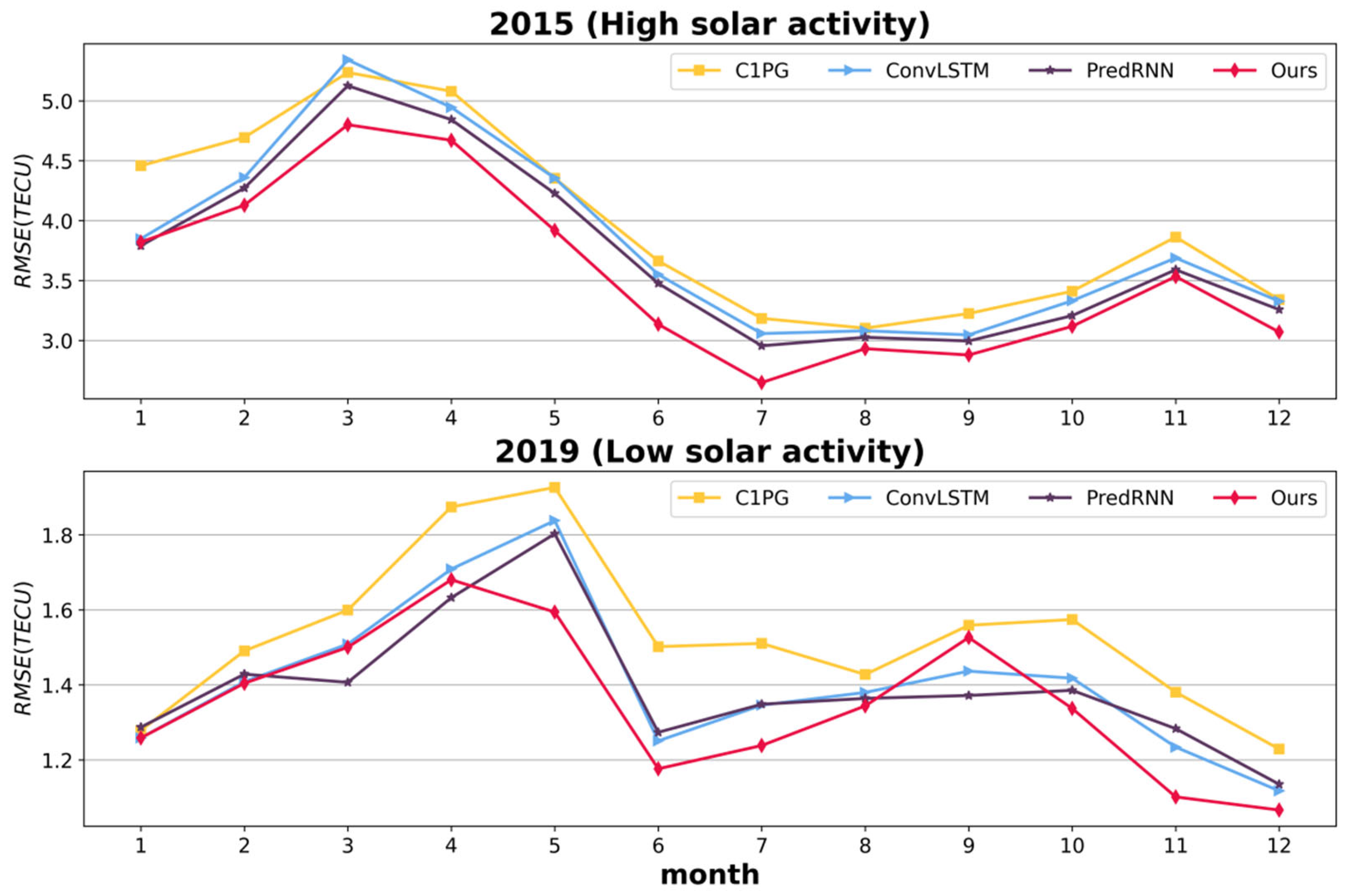
4.4.2. Comparison in Different Months

The previous subsection provided a quantitative comparison from an overall perspective. In contrast, this subsection divides the evaluation period by month, with detailed results presented in Figure 6, with the top and bottom representing the monthly comparisons for 2015 and 2019, respectively.

In 2015, the $RMSE$ of ED-SA-ConvLSTM is consistently the lowest across all months except January. Notably, the advantage of ED-SA-ConvLSTM is very obvious in 7 months (February through July, and December). In 2019, ED-SA-ConvLSTM had the smallest $RMSE$ in 9 months, with particularly notable advantages in May, June, July, November, and December. In March and April, it is inferior to PredRNN, and in September, it is inferior to ConvLSTM and PredRNN. In addition, it can be seen that PredRNN is the second best in the vast majority of cases, due to its dual memory of time and space, which can remember more spatiotemporal changes in history. ED-SA-ConvLSTM is also a dual memory model. In addition to dual memory, ED-SA-ConvLSTM also uses self-attention technology to adaptively weight historical memory to focus on spatial dependencies over long and short distances, making it surpass the PredRNN, which has dual memory in the vast majority of cases.

4.4.3. Comparison at Different Latitude Regions

The previous subsection focused on a temporal comparison, while this subsection will shift to a spatial comparison. To facilitate the spatial analysis, the research area is divided into 10 subregions, each covering a span of 10 degrees of latitude. Figure 7 illustrates the comparisons within each subregion, with the upper depicting the comparison for 2015 and the lower for 2019.

Figure 6 shows that, under both solar activities, the $RMSE$ of each model is highest near the equator and low away from it. This is consistent with the Equatorial Ionization Anomaly (EIA) phenomenon. Additionally, in all cases, the $RMSE$ of the proposed ED-SA-ConvLSTM is lower than that of the comparative models, indicating its superiority over the comparative models.

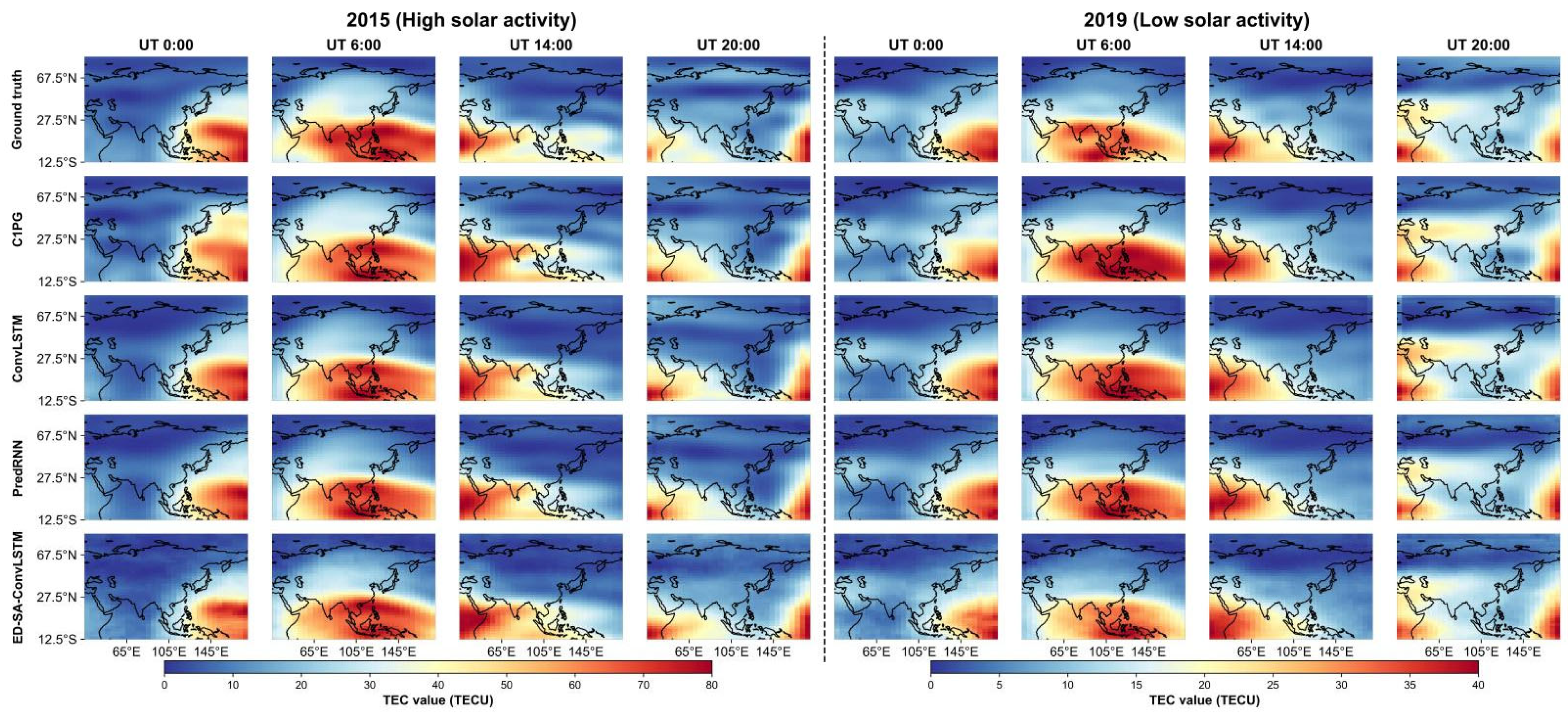
4.4.4. Visual Effects of Various Models

This subsection provides a visual comparison of the prediction effects of ED-SA-ConvLSTM and the three comparative models. We chose one day representing high solar activity (DOY 5, 2015) and another representing low solar activity (DOY 47, 2019) to showcase the performance of each model. The visual effects for each model on the selected days are presented in Figure 8. The corresponding absolute error maps are shown in Figure 9, with the $RMSE$ of each model being annotated at the top of each map and the best highlighted in green. These figures clearly illustrate that ED-SA-ConvLSTM exhibits the smallest area of absolute error anomalies, highlighting its superior predictive performance compared to the other models.

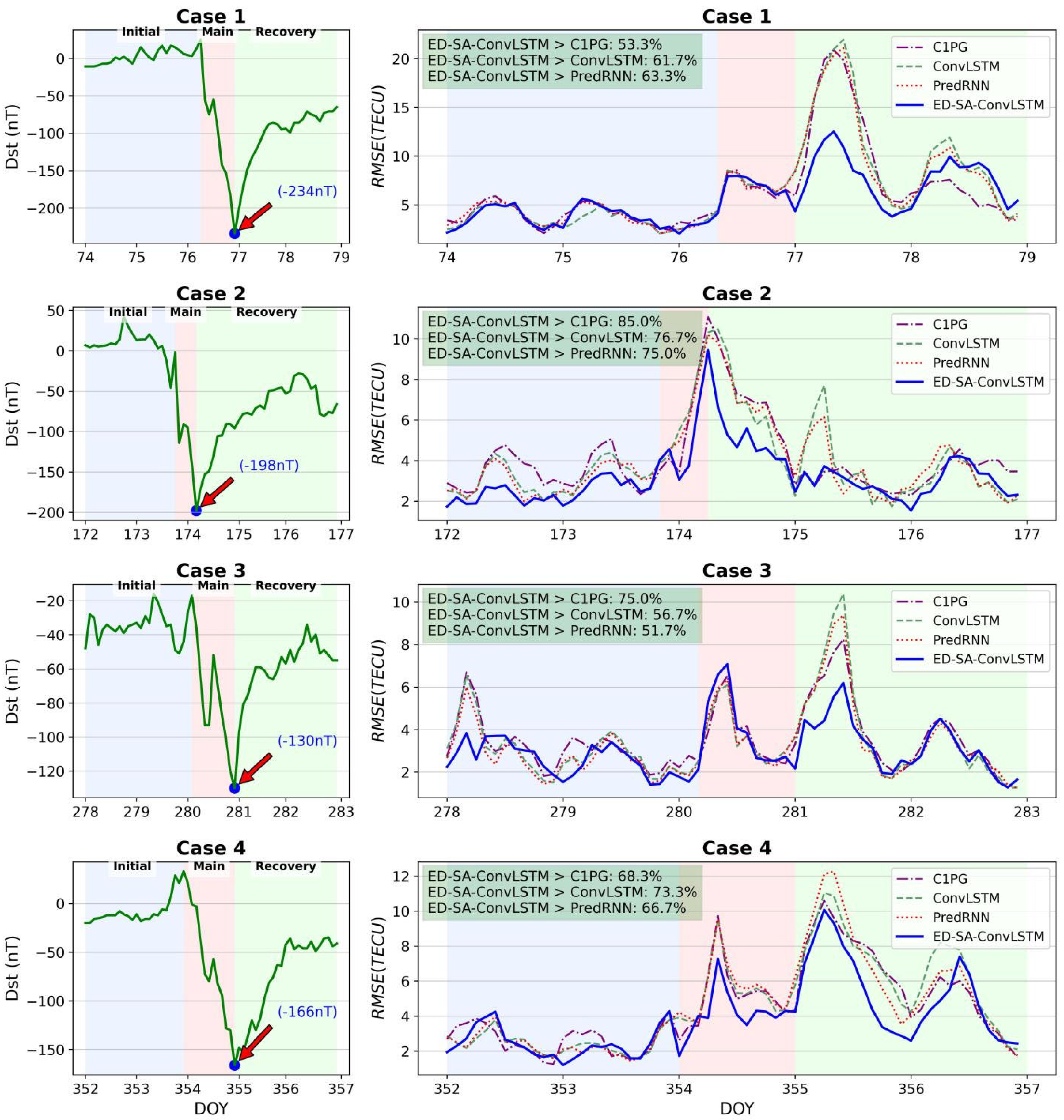
4.5. Comparison Under Extreme Situations

This subsection assesses the effectiveness of the proposed ED-SA-ConvLSTM under extreme conditions. To achieve this, four geomagnetic storm events were selected for analysis. The details of the four selected geomagnetic storm events are presented in

Table 6. Four geomagnetic storm events and their corresponding minimum dst.

Geomagnetic Storm Event	DOY	${\mathit{D}\mathit{s}\mathit{t}}_{\mathit{m}\mathit{i}\mathit{n}}\left(\mathit{n}\mathit{T}\right)$
Case1	DOY 74–78, 2015	−234
Case2	DOY 172–176, 2015	−198
Case3	DOY 278–282, 2015	−130
Case4	DOY 352–356, 2015	−166

.

Figure 10 shows a comparison of the various models across the four geomagnetic storm events. It can be seen that in most cases, the $RMSE$ of the proposed ED-SA-ConvLSTM is lower than those of the comparison models. But there are also some situations that are not as good as comparison models, such as on DOY280 in Case 3.

In summary, the experiments in this subsection prove that ED-SA-ConvLSTM has excellent predictive ability under extreme conditions.

4.6. Comparison Under Other Test Sets

In this subsection, the performance of the proposed ED-SA-ConvLSTM was validated for the years 2011 (high solar activity) and 2016 (low solar activity). The entire region is divided into three parts, namely the low-latitude region (30° N–12.5° S), the mid-latitude region (60° N–30° N), and the high-latitude region (87.5° N–60° N). $RMSE$ and $MAPE$ for each model were calculated separately in these three regions. The results are shown in

Table 7. Each model error in different latitude regions (The best results are bolded).

Solar Activity	Model	Region
		$\mathit{R}\mathit{M}\mathit{S}\mathit{E}\left(\mathit{T}\mathit{E}\mathit{C}\mathit{U}\right)$			$\mathit{M}\mathit{A}\mathit{P}\mathit{E}$
		Low	Mid	High	Low	Mid	High
2011 (high solar activity)	C1PG	3.7699	2.7808	2.3763	11.22%	13.65%	18.92%
	ConvLSTM	3.6902	2.1620	1.9535	10.25%	9.90%	15.91%
	PredRNN	3.6652	2.0896	1.8880	10.00%	9.61%	15.23%
	ED-SA-ConvLSTM	3.5970	1.9606	1.6937	9.92%	9.17%	13.65%
2016 (low solar activity)	C1PG	3.6106	2.3521	1.7489	13.77%	16.22%	22.15%
	ConvLSTM	3.6049	1.9193	1.4531	13.62%	13.02%	20.15%
	PredRNN	3.5372	1.8777	1.3967	13.15%	12.96%	19.53%
	ED-SA-ConvLSTM	3.5631	1.8546	1.3796	13.20%	12.39%	17.87%

. It can be seen that the proposed ED-SA-ConvLSTM outperformed the comparative methods in $RMSE$ and $MAPE$ in low-, mid-, and high-latitude regions in 2011. And in 2016, although PredRNN performed better in the low-latitude region, the proposed ED-SA-ConvLSTM still maintained the lowest errors in the mid- and high-latitude regions. Overall, the proposed ED-SA-ConvLSTM performed better than the comparative models in other years.

4.7. Comparison of Computational Time and Memory Usage

In this subsection, we conducted a quantitative evaluation of the computational time and memory usage for each model, as presented in

Table 8. Computational time and memory usage for each model.

Model	Computational Time (min)	Memory Usage (MB)
ConvLSTM	470	3938.44
PredRNN	675	3954.85
ED-SA-ConvLSTM	1235	3980.18

. C1PG is an official prediction product provided by CODE, so there is no need to calculate the cost. The experimental results demonstrate that the proposed ED-SA-ConvLSTM, which incorporates the self-attention memory module, exhibits significantly higher computational time and memory usage compared to ConvLSTM and PredRNN. However, when combined with the prediction accuracy presented in Section 4.3, Section 4.4 and Section 4.5, ED-SA-ConvLSTM showed superior predictive performance compared to ConvLSTM and PredRNN. This indicates that a moderate investment in computational resources greatly improves prediction accuracy, achieving a balance between accuracy and efficiency.

5. Discussion

The above experiments show that the proposed ED-SA-ConvLSTM is generally superior to the other three state-of-the-art comparison models (C1PG, ConvLSTM, and PredRNN). In 2015, the proposed ED-SA-ConvLSTM reduced $RMSE$ by 10.27%, 7.16%, and 4.53%, respectively; while in 2019, the $RMSE$ reductions were 11.46%, 4.06%, and 2.75%, respectively. In addition, the proposed ED-SA-ConvLSTM exhibits excellent spatiotemporal stability: it maintains optimal performance in 11 months of 2015 and 9 months of 2019, and outperforms the comparison model across 10 regions at different latitudes. We also verified the proposed ED-SA-ConvLSTM under extreme cases. In four magnetic storm events, the proposed ED-SA-ConvLSTM outperformed the comparison models in most cases. Moreover, we tested other solar activity years, namely 2011 (high solar activity) and 2016 (low solar activity). The results indicate that in 2011, the model’s predictive performance was outstanding; In 2016, the performance was slightly inferior to PredRNN. This may be related to the relative amplification of prediction error when TEC value is generally low during periods of low solar activity. Although this model has slightly higher computational time and memory usage than ConvLSTM and PredRNN, comprehensive error analysis shows that this moderate investment of computational resources has resulted in a great improvement in prediction accuracy, achieving a balance between accuracy and efficiency.

6. Conclusions

This paper proposes ED-SA-ConvLSTM, a novel encoder–decoder structure with SA-ConvLSTM units for TEC spatiotemporal prediction. It uniquely integrates dual memory states of temporal and spatial, and a structure similar to self-attention to simultaneously capture short-range memory and long-range memory. This is different from the unique structure of ConvLSTM and PredRNN, which enables it to model complex, dynamic, and long-range spatial dependencies in TEC. Additionally, the encoder–decoder structure used in the proposed model enables it to be applied to spatiotemporal prediction problems with unequal input and output lengths.

In the future, we will focus on optimizing the computational efficiency of the model to reduce processing time and memory usage while maintaining current prediction accuracy. Furthermore, we will explore transferring this model framework to other spatiotemporal prediction domains, including but not limited to solar flare prediction, ionospheric effect simulation during solar eclipses, earthquake precursor monitoring, ionospheric disturbance prediction, and traffic flow prediction across interdisciplinary applications.

References

1. Wang, H.; Liu, H.; Yuan, J.; Le, H.; Shan, W.; Li, L. MAOOA-Residual-Attention-BiConvLSTM: An Automated Deep Learning Framework for Global TEC Map Prediction. Space Weather 2024, 22, e2024SW003954. [Google Scholar] [CrossRef]
2. Gao, X.; Yao, Y. A Storm-Time Ionospheric TEC Model with Multichannel Features by the Spatiotemporal ConvLSTM Network. J. Geod. 2023, 97, 9. [Google Scholar] [CrossRef]
3. Sivavaraprasad, G.; Deepika, V.S.; SreenivasaRao, D.; Ravi Kumar, M.; Sridhar, M. Performance Evaluation of Neural Network TEC Forecasting Models over Equatorial Low-Latitude Indian GNSS Station. Geod. Geodyn. 2020, 11, 192–201. [Google Scholar] [CrossRef]
4. Hu, T.; Lei, Y.; Su, J.; Yang, H.; Ni, W.; Gao, C.; Yu, J.; Wang, Y.; Gu, Y. Learning Spatiotemporal Features of DSA Using 3D CNN and BiConvGRU for Ischemic Moyamoya Disease Detection. Int. J. Neurosci. 2023, 133, 512–522. [Google Scholar] [CrossRef]
5. Wang, D.; Yang, Y.; Ning, S. DeepSTCL: A Deep Spatio-Temporal ConvLSTM for Travel Demand Prediction. In Proceedings of the 2018 International Joint Conference on Neural Networks (IJCNN), Rio de Janeiro, Brazil, 8–13 July 2018; pp. 1–8. [Google Scholar]
6. Wang, X.; Xie, W.; Song, J. Learning Spatiotemporal Features With 3DCNN and ConvGRU for Video Anomaly Detection. In Proceedings of the 2018 14th IEEE International Conference on Signal Processing (ICSP), Beijing, China, 12–16 August 2018; pp. 474–479. [Google Scholar]
7. Bilitza, D. International Reference Ionosphere: Recent Developments. Radio Sci. 1986, 21, 343–346. [Google Scholar] [CrossRef]
8. Bent, R.B.; Llewellyn, S.K.; Nesterczuk, G.; Schmid, P.E. The Development of a Highly-Successful Worldwide Empirical Ionospheric Model and Its Use in Certain Aspects of Space Communications and Worldwide Total Electron Content Investigations; Naval Research Laboratory: Washington, DC, USA, 1975; Volume 1. [Google Scholar]
9. Hochegger, G.; Nava, B.; Radicella, S.; Leitinger, R. A Family of Ionospheric Models for Different Uses. Phys. Chem. Earth Part C Sol. Terr. Planet. Sci. 2000, 25, 307–310. [Google Scholar] [CrossRef]
10. Nava, B.; Coïsson, P.; Radicella, S.M. A New Version of the NeQuick Ionosphere Electron Density Model. J. Atmos. Sol.-Terr. Phys. 2008, 70, 1856–1862. [Google Scholar] [CrossRef]
11. Ansari, K.; Park, K.-D.; Kubo, N. Linear Time-Series Modeling of the GNSS Based TEC Variations over Southwest Japan during 2011–2018 and Comparison against ARMA and GIM Models. Acta Astronaut. 2019, 165, 248–258. [Google Scholar] [CrossRef]
12. Ratnam, D.V.; Otsuka, Y.; Sivavaraprasad, G.; Dabbakuti, J.R.K.K. Development of Multivariate Ionospheric TEC Forecasting Algorithm Using Linear Time Series Model and ARMA over Low-Latitude GNSS Station. Adv. Space Res. 2019, 63, 2848–2856. [Google Scholar] [CrossRef]
13. Vankadara, R.K.; Sasmal, S.; Maurya, A.K.; Panda, S.K. An Autoregressive Integrated Moving Average (ARIMA) Based Forecasting of Ionospheric Total Electron Content at a Low Latitude Indian Location. In Proceedings of the 2022 URSI Regional Conference on Radio Science (USRI-RCRS), Indore, India, 1–4 December 2022; pp. 1–4. [Google Scholar]
14. Jiang, Z.; Zhang, Z.; He, X.; Li, Y.; Yuan, H. Efficient and Accurate TEC Modeling and Prediction Approach with Random Forest and Bi-LSTM for Large-Scale Region. Adv. Space Res. 2024, 73, 650–662. [Google Scholar] [CrossRef]
15. Liu, L.; Zou, S.; Yao, Y.; Wang, Z. Forecasting Global Ionospheric TEC Using Deep Learning Approach. Space Weather 2020, 18, e2020SW002501. [Google Scholar] [CrossRef]
16. Wen, Z.; Li, S.; Li, L.; Wu, B.; Fu, J. Ionospheric TEC Prediction Using Long Short-Term Memory Deep Learning Network. Astrophys Space Sci 2021, 366, 3. [Google Scholar] [CrossRef]
17. Sun, W.; Xu, L.; Huang, X.; Zhang, W.; Yuan, T.; Chen, Z.; Yan, Y. Forecasting of Ionospheric Vertical Total Electron Content (TEC) Using LSTM Networks. In Proceedings of the 2017 International Conference on Machine Learning and Cybernetics (ICMLC), Ningbo, China, 9–12 July 2017; IEEE: Piscataway, NJ, USA, 2017; pp. 340–344. [Google Scholar]
18. Xie, T.; Dai, Z.; Zhu, X.; Chen, B.; Ran, C. LSTM-Based Short-Term Ionospheric TEC Forecast Model and Positioning Accuracy Analysis. GPS Solut. 2023, 27, 66. [Google Scholar] [CrossRef]
19. Tang, J.; Liu, C.; Yang, D.; Ding, M. Prediction of Ionospheric TEC Using a GRU Mechanism Method. Adv. Space Res. 2024, 74, 260–270. [Google Scholar] [CrossRef]
20. Xiong, P.; Zhai, D.; Long, C.; Zhou, H.; Zhang, X.; Shen, X. Long Short-Term Memory Neural Network for Ionospheric Total Electron Content Forecasting Over China. Space Weather 2021, 19, e2020SW002706. [Google Scholar] [CrossRef]
21. Chen, Y.; Liu, H.; Shan, W.; Yao, Y.; Xing, L.; Wang, H.; Zhang, K. Optimizing Deep Learning Models with Improved BWO for TEC Prediction. Biomimetics 2024, 9, 575. [Google Scholar] [CrossRef]
22. Li, D.; Jin, Y.; Wu, F.; Zhao, J.; Min, P.; Luo, X. A Hybrid Model for TEC Prediction Using BiLSTM and PSO-LSSVM. Adv. Space Res. 2024, 74, 303–318. [Google Scholar] [CrossRef]
23. Maheswaran, V.K.; Baskaradas, J.A.; Nagarajan, R.; Anbazhagan, R.; Subramanian, S.; Devanaboyina, V.R.; Das, R.M. Bi-LSTM Based Vertical Total Electron Content Prediction at Low-Latitude Equatorial Ionization Anomaly Region of South India. Adv. Space Res. 2024, 73, 3782–3796. [Google Scholar] [CrossRef]
24. Mao, S.; Li, H.; Zhang, Y.; Shi, Y. Prediction of Ionospheric Electron Density Distribution Based on CNN-LSTM Model. IEEE Geosci. Remote Sens. Lett. 2024, 21, 1–5. [Google Scholar] [CrossRef]
25. Kaselimi, M.; Doulamis, N.; Voulodimos, A.; Doulamis, A.; Delikaraoglou, D. Spatio-Temporal Ionospheric TEC Prediction Using a Deep CNN-GRU Model on GNSS Measurements. In Proceedings of the 2021 IEEE International Geoscience and Remote Sensing Symposium IGARSS, Brussels, Belgium, 11 July 2021; IEEE: Piscataway, NJ, USA, 2021; pp. 8317–8320. [Google Scholar]
26. Ren, X.; Zhao, B.; Ren, Z.; Wang, Y.; Xiong, B. Deep Learning-Based Prediction of Global Ionospheric TEC During Storm Periods: Mixed CNN-BiLSTM Method. Space Weather 2024, 22, e2024SW003877. [Google Scholar] [CrossRef]
27. Lei, D.; Liu, H.; Le, H.; Huang, J.; Yuan, J.; Li, L.; Wang, Y. Ionospheric TEC Prediction Base on Attentional BiGRU. Atmosphere 2022, 13, 1039. [Google Scholar] [CrossRef]
28. Han, C.; Guo, Y.; Ou, M.; Wang, D.; Song, C.; Jin, R.; Zhen, W.; Bai, P.; Chong, X.; Wang, X. A Lightweight Prediction Model for Global Ionospheric Total Electron Content Based on Attention-BiLSTM. Adv. Space Res. 2024, 75, 3614–3629. [Google Scholar] [CrossRef]
29. Liu, H.; Wang, H.; Yuan, J.; Li, L.; Zhang, L. TEC Prediction Based on Att-CNN-BiLSTM. IEEE Access 2024, 12, 68471–68484. [Google Scholar] [CrossRef]
30. Shi, X.; Chen, Z.; Wang, H.; Yeung, D.-Y.; Wong, W.; WOO, W. Convolutional LSTM Network: A Machine Learning Approach for Precipitation Nowcasting. In Proceedings of the Advances in Neural Information Processing Systems, Montreal, QC, Canada, 7–12 December 2015; Curran Associates, Inc.: Red Hook, NY, USA, 2015; Volume 28. [Google Scholar]
31. Chen, J.; Zhi, N.; Liao, H.; Lu, M.; Feng, S. Global Forecasting of Ionospheric Vertical Total Electron Contents via ConvLSTM with Spectrum Analysis. GPS Solut. 2022, 26, 69. [Google Scholar] [CrossRef]
32. Liu, L.; Morton, Y.J.; Liu, Y. ML Prediction of Global Ionospheric TEC Maps. Space Weather 2022, 20, e2022SW003135. [Google Scholar] [CrossRef]
33. Xu, C.; Ding, M.; Tang, J. Prediction of GNSS-Based Regional Ionospheric TEC Using a Multichannel ConvLSTM With Attention Mechanism. IEEE Geosci. Remote Sens. Lett. 2024, 21, 1–5. [Google Scholar] [CrossRef]
34. Li, L.; Liu, H.; Le, H.; Yuan, J.; Shan, W.; Han, Y.; Yuan, G.; Cui, C.; Wang, J. Spatiotemporal Prediction of Ionospheric Total Electron Content Based on ED-ConvLSTM. Remote Sens. 2023, 15, 3064. [Google Scholar] [CrossRef]
35. de Paulo, M.C.M.; Marques, H.A.; Feitosa, R.Q.; Ferreira, M.P. New Encoder–Decoder Convolutional LSTM Neural Network Architectures for next-Day Global Ionosphere Maps Forecast. GPS Solut. 2023, 27, 95. [Google Scholar] [CrossRef]
36. Yang, J.; Huang, W.; Xia, G.; Zhou, C.; Chen, Y. Operational Forecasting of Global Ionospheric TEC Maps 1-, 2-, and 3-Day in Advance by ConvLSTM Model. Remote Sens. 2024, 16, 1700. [Google Scholar] [CrossRef]
37. Li, L.; Liu, H.; Le, H.; Yuan, J.; Wang, H.; Chen, Y.; Shan, W.; Ma, L.; Cui, C. ED-AttConvLSTM: An Ionospheric TEC Map Prediction Model Using Adaptive Weighted Spatiotemporal Features. Space Weather 2024, 22, e2023SW003740. [Google Scholar] [CrossRef]
38. Tang, J.; Zhong, Z.; Ding, M.; Yang, D.; Liu, H. Forecast of Ionospheric TEC Maps Using ConvGRU Deep Learning Over China. IEEE J. Sel. Top. Appl. Earth Obs. Remote Sens. 2024, 17, 3334–3344. [Google Scholar] [CrossRef]
39. Liu, H.; Wang, H.; Le, H.; Yuan, J.; Shan, W.; Wu, Y.; Chen, Y. CGAOA-STRA-BiConvLSTM: An Automated Deep Learning Framework for Global TEC Map Prediction. GPS Solut. 2025, 29, 55. [Google Scholar] [CrossRef]
40. Tang, J.; Zhong, Z.; Hu, J.; Wu, X. Forecasting Regional Ionospheric TEC Maps over China Using BiConvGRU Deep Learning. Remote Sens. 2023, 15, 3405. [Google Scholar] [CrossRef]
41. Luo, W.; Li, Y.; Urtasun, R.; Zemel, R. Understanding the Effective Receptive Field in Deep Convolutional Neural Networks. Adv. Neural Inf. Process. Syst. 2016, 29. Available online: https://proceedings.neurips.cc/paper/2016/hash/c8067ad1937f728f51288b3eb986afaa-Abstract.html (accessed on 11 June 2025).
42. Wang, Y.; Long, M.; Wang, J.; Gao, Z.; Yu, P.S. PredRNN: Recurrent Neural Networks for Predictive Learning Using Spatiotemporal LSTMs. Adv. Neural Inf. Process. Syst. 2017, 30. Available online: https://proceedings.neurips.cc/paper/2017/hash/e5f6ad6ce374177eef023bf5d0c018b6-Abstract.html?ref=https://githubhelp.com (accessed on 11 June 2025).
43. Lin, Z.; Li, M.; Zheng, Z.; Cheng, Y.; Yuan, C. Self-Attention ConvLSTM for Spatiotemporal Prediction. Proc. AAAI Conf. Artif. Intell. 2020, 34, 11531–11538. [Google Scholar] [CrossRef]
44. Badrinarayanan, V.; Kendall, A.; Cipolla, R. SegNet: A Deep Convolutional Encoder-Decoder Architecture for Image Segmentation. IEEE Trans. Pattern Anal. Mach. Intell. 2017, 39, 2481–2495. [Google Scholar] [CrossRef]
45. Chen, L.-C.; Zhu, Y.; Papandreou, G.; Schroff, F.; Adam, H. Encoder-Decoder with Atrous Separable Convolution for Semantic Image Segmentation. In Proceedings of the European Conference on Computer Vision (ECCV), Munich, Germany, 8–14 September 2018; pp. 801–818. [Google Scholar]
46. Cho, K.; Merrienboer, B.v.; Gulcehre, C.; Bahdanau, D.; Bougares, F.; Schwenk, H.; Bengio, Y. Learning Phrase Representations Using RNN Encoder-Decoder for Statistical Machine Translation. In Proceedings of the 2014 Conference on Empirical Methods in Natural Language Processing (EMNLP), Doha, Qatar, 25–29 October 2014. [Google Scholar]
47. Elman, J.L. Finding Structure in Time. Cogn. Sci. 1990, 14, 179–211. [Google Scholar] [CrossRef]
Figure 1. Generate TEC dataset using sliding window.
Mathematics 13 01986 g001
Figure 2. The structure of a SAM module.
Mathematics 13 01986 g002
Figure 3. Structure of a SA-ConvLSTM unit.
Mathematics 13 01986 g003
Figure 4. Structure of ED-SA-ConvLSTM.
Mathematics 13 01986 g004
Figure 5. Influence of input length on the model’s prediction performance.
Mathematics 13 01986 g005
Figure 6. Monthly comparison among all models.
Mathematics 13 01986 g006
Figure 7. Comparison of each model in each subregion.
Mathematics 13 01986 g007
Figure 8. TEC prediction maps in 2015 and in 2019 for each model.
Mathematics 13 01986 g008
Figure 9. Absolute error maps for 2015 and for 2019 for each model.
Mathematics 13 01986 g009
Figure 10. Comparison on four magnetic storm events.
Mathematics 13 01986 g010