Improved Fuel Consumption Estimation for Sailing Speed Optimization: Eliminating Log Transformation Bias

Abstract

Sailing Speed Optimization (SSO) is a crucial problem in shipping operations management, aiming to reduce both operating costs and carbon dioxide emissions. The ship’s sailing speed directly impacts fuel consumption, where fuel consumption is generally assumed to follow a power function with respect to sailing speed. Previous studies have used transformation-based fitting methods, such as logarithmic transformations, to investigate the relationship between sailing speed and fuel consumption using historical data. However, these methods introduce estimation bias and heteroskedasticity, violating the core assumptions of Ordinary Least Squares (OLS) used for general linear regression. To address these issues, we propose two novel fitting methods that directly optimize the original nonlinear model without relying on transformations. By analyzing the characteristics of the objective function, we derive parameter constraints and integrate them into a discrete optimization framework, resulting in improved fitting accuracy. Our methods are validated through extensive case studies, demonstrating their effectiveness in enhancing the reliability of SSO decisions. These methods offer a practical approach to optimizing fuel consumption in real-world maritime operations.

1. Introduction

Sailing Speed Optimization (SSO) is a typical optimization problem that plays a crucial role in shipping operations management, which can reduce both total operating costs and carbon dioxide (CO₂) emissions [1]. The core decision variable in SSO is the ship’s sailing speed, which has a direct and substantial impact on bunker consumption. The fuel consumption of a ship is highly sensitive to its speed; specifically, daily bunker consumption is approximately proportional to the third power of the sailing speed [2]. Bunker costs represent a significant portion of total operating expenses, ranging from 20% to 60% [3]. Furthermore, according to the International Maritime Organization (IMO) [4], in 2018, international shipping emitted 1056 million tons of CO₂, accounting for about 2.89% of global emissions. Most of the emissions come from the combustion of fossil fuels [5]. Therefore, determining an optimal sailing speed is essential for achieving both economic and environmental benefits in maritime operations [6,7].

Previous studies have extensively explored the modeling methods of SSO and designed corresponding solution algorithms. To quantify the impact of speed on fuel consumption, establishing an accurate relationship between bunker consumption and sailing speed has become a key challenge in SSO. Although machine learning methods have been widely applied to construct predictive models for bunker consumption, the resulting black-box models often lack interpretability [8]. In many cases, even domain experts in the maritime industry find it difficult to explain the outcomes of such models. This lack of transparency can make shipping company managers hesitant to adopt them in practice due to perceived risks. Therefore, it remains of significant research value to represent the relationship between relevant variables using explicit domain knowledge-based functional expressions [9].

A widely used method involves fitting functional relationships—often linearized through logarithmic transformations for nonlinear forms such as power functions—and embedding them into optimization models [1,10,11,12]. However, logarithmic transformation has limitations, as it may introduce estimation bias, especially when the original error structure is distorted during linearization. We show that applying logarithmic transformation to the model introduces heteroskedasticity, where the variance of the error term changes with the magnitude of the independent variable. This violates the core assumption of Ordinary Least Squares (OLS) used for linear regression, which assumes homoskedasticity (constant variance). Therefore, proposing a more accurate parameter estimation method is of significant research interest, as it can further enhance the reliability of fuel consumption modeling and improve the overall performance of SSO [13,14,15].

In this paper, we develop an SSO model and design a corresponding solution algorithm. To overcome the limitations of logarithmic transformation, we propose two novel fitting methods that optimize the OLS objective function without relying on transformation techniques. Through an in-depth analysis of the objective function, we derive constraint relationships among the fitting parameters, which are then embedded into the objective for discrete optimization. Two methods are proposed: gradient substitution search (GSS), which simplifies the system via partial derivatives and discrete enumeration, and constrained nonlinear optimization (CNO), which directly solves the objective under parameter constraints. These methods not only improve fitting accuracy but also enhance the reliability of downstream decision-making in SSO. The effectiveness of our proposed methods is extensively validated through a large number of numerical experiments. The core contributions of this paper lie in the following:

• We provide a theoretical analysis that rigorously demonstrates the mathematical limitations of logarithmic transformation when applied to OLS estimation, revealing its inherent biases and restricted applicability in nonlinear settings.
• We propose two novel estimation approaches that directly optimize the original OLS objective function without resorting to transformation techniques, thereby offering more robust and interpretable parameter estimates.
• We apply the proposed methods to a structured SSO problem, where comprehensive numerical experiments validate their superior fitting accuracy and improved reliability in downstream decision-making tasks.

The remainder of this paper is organized as follows: Section 2 reviews related work in the field. Section 3 introduces the SSO problem and outlines the proposed solution algorithm. Section 4 discusses the limitations of logarithmic transformation and presents two direct, data-driven estimation methods for nonlinear models. Section 5 reports the results of numerical experiments. Finally, Section 6 concludes the paper.

2. Literature Review

SSO aims to determine the optimal sailing speed that minimizes fuel consumption or operating costs while satisfying transport schedules and operational constraints. To obtain the optimal speed, a key issue lies on how to build an accurate vessel fuel consumption prediction model [16]. Many studies have shown that the sailing speed determines the bunker consumption and that the vessel fuel consumption is proportional to the $\alpha$-th power of the sailing speed, where $\alpha$ is estimated by regression analysis [10,12,17]. Under this assumption, Fagerholt et al. [10] developed a nonlinear model for segment-wise optimal speeds along shipping routes, and later discretized and solved this model using the shortest path algorithm. Kim et al. [11] introduced an exact solution for the same problem. Yao et al. [1] incorporated empirical speed–bunker consumption relationships for different container ship sizes into a model optimizing refueling decisions and sailing speeds. Similarly, Wang and Meng [12] used historical data to build a mixed-integer nonlinear model optimizing speeds for multiple vessels in a liner network.

With the widespread use of sensors, data availability in the maritime domain has significantly increased, enabling the more accurate modeling of ship fuel consumption. Recent studies have increasingly applied machine learning techniques to incorporate various influencing factors into fuel consumption prediction. Tarelko and Rudzki [18] developed two artificial neural network models to predict fuel consumption, which were then used in a bi-objective optimization model targeting reduced fuel use and increased sailing speed. Du et al. [19] proposed a two-phase approach: using artificial neural network models to build the function between bunker consumption and sailing speed from noon reports, followed by the optimization of speed to minimize fuel consumption. Furthermore, Le et al. [20] developed a black-box multilayer perceptron artificial neural network to predict ship fuel consumption and demonstrated its superior performance over two white-box regression models. Yan et al. [21] adopted random forest to predict ship fuel consumption and optimized the ship’s sailing speed based on the predicted results. Uyanik et al. [22] developed a decision tree model and neural network model to predict ship fuel consumption.

Table 1. Summary of estimation and modeling approaches for SSO.

Reference	Method Type	Modeling Approach and Application
Fagerholt et al. (2010) [10]	Physics-based	Power-law function and nonlinear model for segment-wise optimal sailing speed
Yao et al. (2012) [1]	Physics-based	Empirical speed–fuel formulas by ship size for joint bunkering and speed optimization
Wang and Meng (2012) [12]	Physics-based	Mixed-integer nonlinear programming for speed optimization of multiple vessels in liner networks
Kim et al. (2016) [11]	Physics-based	Exact solution method for segment-wise optimal sailing speed
Du et al. (2019) [19]	Machine Learning	Artificial neural network-based two-phase approach for speed optimization using noon report data
Tarelko and Rudzki (2020) [18]	Physics-based	Artificial neural networks for bi-objective optimization (fuel consumption vs. speed)
Le et al. (2020) [20]	Machine Learning	Multilayer perceptron and regression models for fuel consumption prediction
Yan et al. (2020) [21]	Machine Learning	Random forest for fuel consumption prediction and speed optimization
Uyanik et al. (2023) [22]	Machine Learning	Develop decision tree model and neural network model to predict ship fuel consumption

summarizes these methods.

Despite the promising performance of machine learning methods, their lack of interpretability often hinders their practical adoption. Black-box models, such as neural networks, produce results that even maritime experts find difficult to explain. As a result, frontline staff and decision-makers in shipping companies are often reluctant to trust and apply these models. Therefore, developing interpretable functional relationships between input factors and fuel consumption remains practically valuable and necessary for real-world implementation. For transformation-based fitting methods, Shangguan et al. [23] revealed a key limitation: if the transformed samples used in linear regression are not strictly linearly correlated, the resulting parameter estimates tend to be biased. In this paper, we further demonstrate that such transformations can introduce heteroskedasticity into the model, thereby violating the fundamental assumptions of OLS used for linear regression and leading to unreliable estimation results. To address these challenges, we propose two new fitting methods that do not need transformation procedures and directly optimize the original nonlinear model, improving fitting accuracy while maintaining interpretability. Case studies confirm their effectiveness in improving SSO decisions.

3. Problem Formulation and Algorithm Design

In this section, we introduce the SSO problem and develop the corresponding mathematical model. We then present a solution approach based on the bisection algorithm.

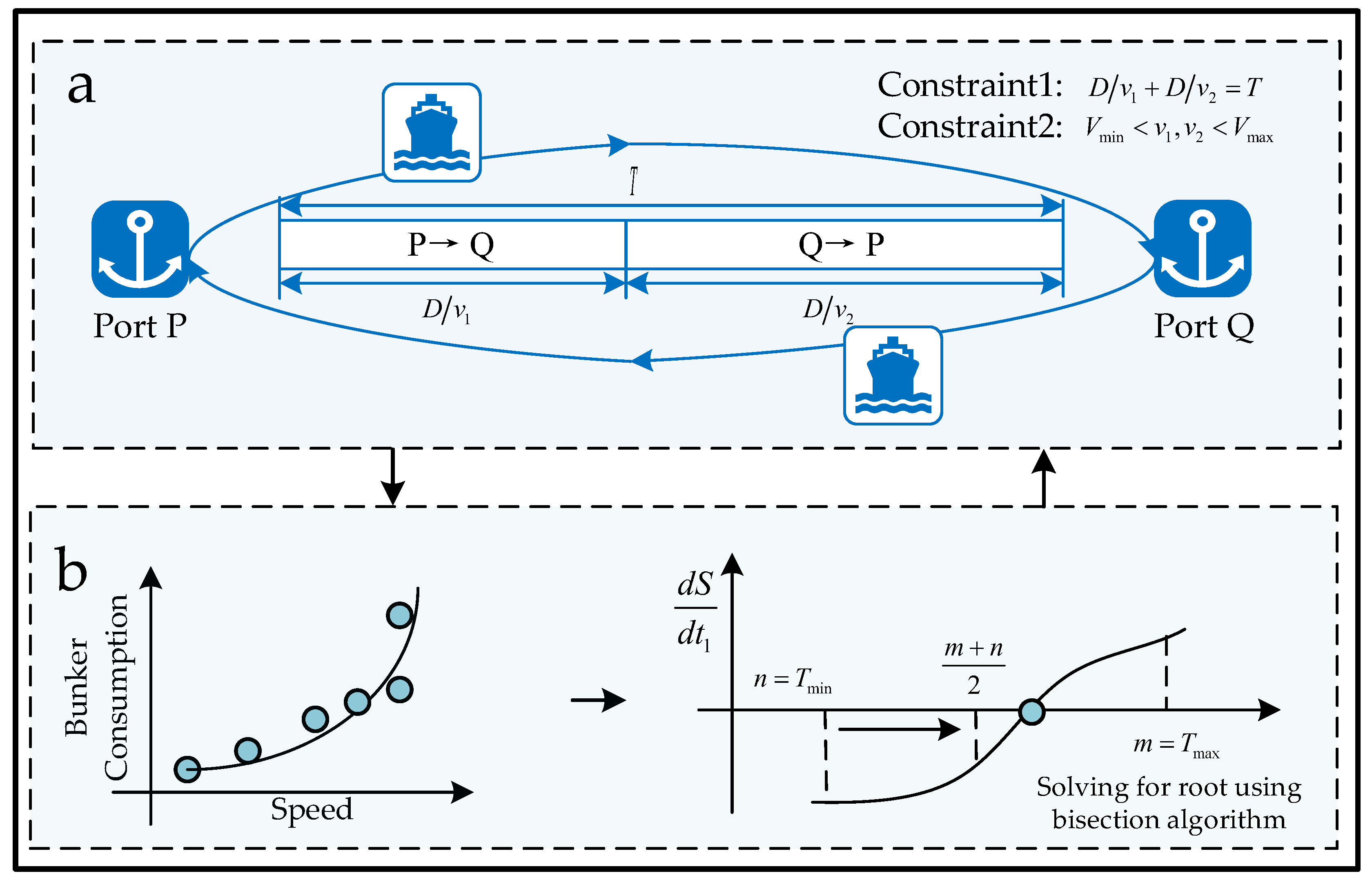
3.1. Sailing Speed Optimization Model

As shown in Figure 1a, the objective of the SSO problem is to determine the optimal sailing speeds (in knots) that minimize bunker fuel consumption for vessel operations between two ports, P and Q. The sailing distance between ports P and Q is denoted as $D$ (in nautical miles). Considering distinct environmental factors such as ocean currents, weather patterns, and cargo load variations in outbound and return voyages, the bunker consumption cost functions (in tons per day) exhibit directional asymmetry between the P-Q and Q-P voyages. These are, respectively, denoted as $g_1(v_1)$ for the outbound voyage (P→Q) and $g_2(v_2)$ for the return voyage (Q→P), where $v_1$ and $v_2$ serve as decision variables, representing the vessel’s speed for each voyage of the journey, respectively. According to previous studies and domain knowledge, the bunker consumption cost functions, $g_1(v_1)$ and $g_2(v_2)$, generally follow power-law relationships:

$$g_1(v_1)={a_1{v}_1}^{b_1},$$

(1)

$$g_2(v_2)={a_2{v}_2}^{b_2},$$

(2)

where $a_1$, $a_2$, $b_1$, and $b_2$ are the function parameters to be estimated. In Section 4, we will elaborate on how to estimate these parameters using historical data. Furthermore, the complete round-trip voyage must be accomplished within the time window $T$ (in hours). To ensure ship safety and schedule reliability, the vessel speed is bounded between $V_{\min }$ and $V_{\max }$. The objective function is denoted by $S$, which is derived by multiplying the fuel consumption rate $g_i(v_i)$, $i=1,2$, with the travel time $D/v_i$, $i=1,2$, for each leg of the voyage. The two segments are then summed to obtain the total fuel usage. A factor of $1/24$ is applied to normalize the cost into a daily scale. The mathematical model is formulated as follows:

$$\underset{v_1,v_2}{\min }\left\{S=g_1\left(v_1\right)\cdot {\displaystyle \frac{D}{24v_1}}+g_2\left(v_2\right)\cdot {\displaystyle \frac{D}{24v_2}}\right\}$$

(3)

subject to

$${\displaystyle \frac{D}{v_1}}+{\displaystyle \frac{D}{v_2}}=T$$

(4)

$$V_{\min }\le v_1,v_2\le V_{\max }$$

(5)

Objective function (3) minimizes the total bunker consumption, and the factor 24 in objective function (3) serves to convert hours into days, thereby ensuring dimensional consistency. Constraint (4) ensures that the sum of the sailing times from P to Q and from Q to P is a constant value. Constraint (5) ensures the vessel speeds should be no less than $V_{\min }$ and no more than $V_{\max }$, where $V_{\min }$ is the minimum vessel speed value and $V_{\max }$ is the maximum vessel speed value.

In the solution process, it is difficult to directly optimize sailing speeds because they appear in the denominator for calculating the sailing time, leading to a nonlinear constraint, as indicated in Constraint (4). Thus, we transform sailing speeds into travel times by defining $t_1=D/v_1$ and $t_2=D/v_2$. Then, by substituting the expressions for $v_1=D/t_1$ and $v_2=D/t_2$ into Equation (3), we obtain a reformulated objective function. Considering that the vessel speed is bounded between $V_{\min }$ and $V_{\max }$, the corresponding travel time is also constrained, given by $T_{\min }=D/V_{\max }$ and $T_{\max }=D/V_{\min }$. Thus, both $t_1$ and $t_2$ must remain within the operationally acceptable time interval $[T_{\min },T_{\max }]$. Therefore, the above model is transformed into

$$\underset{t_1,t_2}{\min }\left\{S=g_1\left({\displaystyle \frac{D}{t_1}}\right)\cdot {\displaystyle \frac{t_1}{24}}+g_2\left({\displaystyle \frac{D}{t_2}}\right)\cdot {\displaystyle \frac{t_2}{24}}\right\}$$

(6)

subject to

$$t_1+t_2=T$$

(7)

$$T_{\min }\le t_1,t_2\le T_{\max }.$$

(8)

3.2. Solving the SSO Model

Figure 1b provides the visual representation of the solution algorithm. To solve this model, we plug Equations (1) and (2) into objective function (6) and obtain

$$S={\displaystyle \frac{1}{24}}\cdot \left[a_1{t}_1\cdot {(D/t_1)}^{b_1}+a_2{t}_2\cdot {(D/t_2)}^{b_2}\right]={\displaystyle \frac{1}{24}}\cdot \left[a_1{D}^{b_1}\cdot {t_1}^{-b_1+1}+a_2{D}^{b_2}\cdot {t_2}^{-b_2+1}\right].$$

(9)

Plugging $t_2=T-t_1$ into (9), we obtain

$$S={\displaystyle \frac{1}{24}}\left[a_1{D}^{b_1}\cdot {t_1}^{-b_1+1}+a_2{D}^{b_2}\cdot {t_2}^{-b_2+1}\right]={\displaystyle \frac{1}{24}}\left[a_1{D}^{b_1}\cdot {t_1}^{-b_1+1}+a_2{D}^{b_2}\cdot {\left(T-t_1\right)}^{-b_2+1}\right].$$

(10)

To find the optimal value of $t_1$ that minimizes the objective function value, we compute the derivative of $S$ with respect to $t_1$ and set it equal to 0:

$${\displaystyle \frac{dS}{d{t}_1}}={\displaystyle \frac{1}{24}}\left[\left(-b_1+1\right)a_1{D}^{b_1}{t}_1^{-b_1}+\left(b_2-1\right)a_2{D}^{b_2}{(T-t_1)}^{-b_2}\right]=0.$$

(11)

This constitutes a nonlinear equation that typically requires numerical optimization methods for obtaining the optimal solution. To verify that the root of Equation (11) corresponds to a minimum (rather than a maximum or saddle point), we may examine the second-order derivative of $S$ with respect to $t_1$ to analyze its convexity. The second-order derivative of $S$ with respect to $t_1$ is

$${\displaystyle \frac{d^{2}S}{d{t_1}^2}}={\displaystyle \frac{1}{24}}\left[\left(b_1-1\right)b_1{a}_1{D}^{b_1}{t}_1^{-b_1-1}+\left(b_2-1\right)b_2{a}_2{D}^{b_2}{(T-t_1)}^{-b_2-1}\right].$$

(12)

when $b_1,b_2>1$, the function $S(t_1)$ is convex over the domain $t_1\in \left[0,T\right]$, since (12) is non-negative. In SSO, because daily bunker consumption is approximately proportional to the third power of the sailing speed, $b_1,b_2>1$ is satisfied. Plugging $t_2=T-t_1$ into Constraint (8), we obtain $T-T_{\max }\le t_1\le T-T_{\min }$. Therefore, the domain of $t_1$ is

$$\max \left\{T_{\min },T-T_{\max }\right\}\le t_1\le \min \left\{T_{\max },T-T_{\min }\right\}.$$

(13)

Consequently, the optimal value $t_1^{*}$ at which the first-order derivative equals zero represents the global minimum. However, since an optimal solution is difficult to obtain in an analytical manner due to the complexity of the function, a numerical method is required. Among various numerical algorithms, the bisection method is chosen due to its simplicity, robustness, and guaranteed convergence for continuous functions with sign changes [24]. We apply the bisection method to find the optimal solution, as illustrated in

Table 2. Bisection algorithm to search for the approximate root of Equation (11).

Input: Define $f(t_1)=ds/d{t}_1$  Using Equation(11), Total Schedule Time $T$, Interval $T_{\min },T_{\max }$, Tolerance ${\xi }_1$, and ${\xi }_2$.
Output: The optimal value $t_1^{*}$.
1	Set $m=\max \left\{T_{\min },T-T_{\max }\right\}$, and $n=\min \left\{T_{\max },T-T_{\min }\right\}$ as the initial upper and lower bounds
2	If $f(m)\cdot f(n)>0$: (i.e., a root does not exist in the interval)
3	If $f\left(m\right)>0$:
4	Return $t_1^{*}$ = $m$
5	Else:
6	Return $t_1^{*}$ = $n$
7	Else: (i.e., a root exists in the interval)
8	While True:
9	Compute midpoint $r={\displaystyle \frac{m+n}{2}}$.
10	Compute $f\left(r\right)$.
11	If $f(r)<{\xi }_1$ or $|m-n|<{\xi }_2$:
12	Return $t_1^{*}$ = $r$, End while loop.
13	Else if $f(m)\cdot f(r)<0$,
14	Set $n=r$.
15	Else:
16	Set $m=r$.
17	Output: Return $t_1^{*}$ as the approximate root.

. Now, solving the SSO model hinges on the estimated parameters in Equations (1) and (2), which will be discussed in detail in the following section.

4. Limitations of Logarithmic Transformation and Direct Estimation Methods

This section highlights the limitations of logarithmic transformation and introduces two novel models that estimate the parameters directly, eliminating the need for logarithmic conversion.

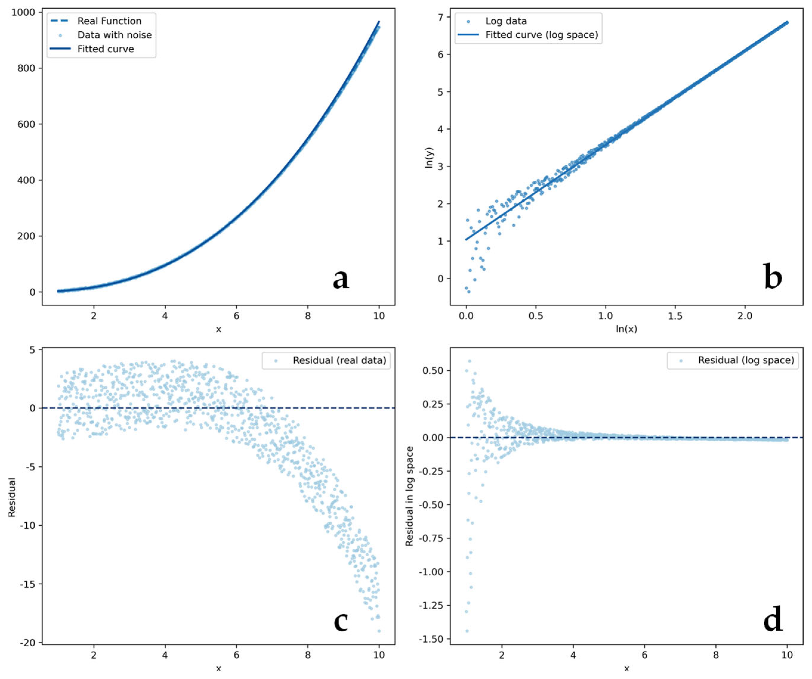
4.1. Limitations of Log Transformation

OLS is widely used in data analysis to estimate the parameters of a function that minimizes the squared error between the predicted and observed data. This function is generally a linear function. When the function is nonlinear, the common strategy is to transform the nonlinear function into a linear function, if possible. We assume there are two random variables, $X$ and $Y$. In this paper, the variable $X$ represents the speed, while $Y$ denotes the bunker consumption. Thus, $Y$ is determined by the relationship:

$$Y=a{X}^b+ϵ,$$

(14)

where $a$ and $b$ are function parameters, and $ϵ$ is the error variable that is assumed to follow a distribution with a mean 0 and variance ${\sigma }^2$. We sample $N$ times from the joint distribution of $X$ and $Y$ independently to obtain the corresponding training set ${\{(x_i,y_i)\}}_{i=1}^N$. In the case study, the training data is also generated following the same procedure described above. The aim of OLS is to estimate the values of $a$ and $b$ from the observed training set. We need to solve the following optimization model:

$$\underset{a,b}{\min }{\displaystyle \frac{1}{N}}\hspace{0.33em}{\displaystyle \sum }_{i=1}^N{\left(y_i-a{x}_i^b\right)}^2.$$

(15)

Considering the nonlinear form of Equation (14), we first conduct the logarithmic transformation, which means taking the logarithm of both $y_i$ and $a{x}_i^b$. Thus, objective function (15) is transformed into

$$\underset{a,b}{\min }{\displaystyle \frac{1}{N}}\hspace{0.33em}{\displaystyle \sum }_{i=1}^N{\left(\ln y_i-\ln a-b\ln x_i\right)}^2.$$

(16)

According to the Gauss–Markov theorem [25], the error term in the OLS should satisfy the assumption of homoskedasticity, meaning that $ϵ$ does not depend on $X$. However, as indicated below, this assumption is not satisfied due to the logarithmic transformation.

We define the new error term as ${ϵ}^{\prime }$ after the logarithmic transformation, which is calculated as follows:

$${ϵ}^{\prime }=\ln Y-\ln a-b\ln X=\ln (a{X}^b+ϵ)-\ln a-b\ln X.$$

(17)

Expanding the Taylor approximation to (17) (assuming $ϵ\ll a{X}^b$), Formula (17) can be transformed into

$${ϵ}^{\prime }\approx \ln (a{X}^b)+{\displaystyle \frac{ϵ}{a{X}^b}}-\ln (a{X}^b)={\displaystyle \frac{ϵ}{a{X}^b}}.$$

(18)

Thus, we derive

$${ϵ}^{\prime }~\left(0,{\displaystyle \frac{{\sigma }^2}{{(a{X}^b)}^2}}\right).$$

(19)

Obviously, ${ϵ}^{\prime }$ is heteroskedastic, which means that the variance of the error term changes with the independent variable $X$. Thus, Functions (15) and (16) are not equivalent due to the logarithmic transformation. The error term ${ϵ}^{\prime }$ is inversely proportional to $X^{2b}$, as indicated in Equation (19). Each error term is weighted with respect to the corresponding $X$. Samples with larger values of $X$ are given lower weights, leading to a poorer fit for them and reducing their influence on the overall model.

We further discuss the solution of Model (16). Let $Q$ be the objective function of (16). We take the partial derivatives of $Q$ with respect to $a$ and $b$, respectively, and obtain

$${\displaystyle \frac{\partial Q}{\partial a}}={\displaystyle \frac{2{\displaystyle \sum _{i=1}^N\left(\ln y_i-\ln a-b\cdot \ln x_i\right)}}{N\cdot a}},$$

(20)

$${\displaystyle \frac{\partial Q}{\partial b}}={\displaystyle \frac{2}{N}}{\displaystyle \sum _{i=1}^N\left[\ln y_i\ln x_i-\ln a\ln x_i-b\cdot {\left(\ln x_i\right)}^2\right]}.$$

(21)

Letting (20) and (21) equal 0, we obtain the optimal estimation parameters:

$$\widehat{b}={\displaystyle \frac{{\displaystyle \sum _{i=1}^N\left(\ln x_i\cdot \ln y_i\right)}-\frac{1}{N}\left({\displaystyle \sum _{i=1}^N\ln x_i}\right)\cdot \left({\displaystyle \sum _{i=1}^N\ln y_i}\right)}{{\displaystyle \sum _{i=1}^N{\left(\ln x_i\right)}^2}-\frac{1}{N}{\left({\displaystyle \sum _{i=1}^N\ln x_i}\right)}^2}},$$

(22)

$$\widehat{a}={\displaystyle \frac{1}{N}}{\displaystyle \sum _{i=1}^N\ln y_i}-\widehat{b}{\displaystyle \frac{1}{N}}{\displaystyle \sum _{i=1}^N\ln x_i}.$$

(23)

It can be proved that if $Y=a+b\ln X+ϵ$, the estimations are unbiased, because they fit the assumption of OSL. However, in this paper, we have $\ln (Y)=\ln (a{X}^b+ϵ)$, indicating that there is a high probability that these estimates are biased. We also use a simple numerical example to illustrate these limitations in Example 1.

Example 1. 

Heteroskedasticity in Synthetic Data Fitting.

We generate a set of synthetic data by setting $a=3$, $b=2.5$, and ${\sigma }^2=5$. $x_i$ ($i\in \{1,\dots ,N\}$) is randomly selected from $U[1,10]$, with $N=1000$. The generated data can be seen in Figure 2a. Then, we use the logarithmic transformation estimation method to obtain the estimated parameters. Figure 2b presents the data and the fitted curve in logarithmic space (taking logarithms of both $y$ and $x$). To further discuss the effect of logarithmic transformation, we give the residual analysis in real data (Figure 2c) and after logarithmic transformation (Figure 2d), respectively. Obviously, after logarithmic transformation, the residual variance is larger for the data with a smaller $x$. Since the regression is conducted in the logarithmic space by minimizing the squared residuals, these high-variance samples contribute more significantly to the loss function. As a result, the model tends to focus more on fitting data samples in the smaller range of $x$, potentially at the expense of accuracy in the larger range of $x$. Therefore, when translated back into the original data space, this fitting process leads to the pattern observed in Figure 2c—the residuals tend to increase with larger $x$ values. Although the model emphasizes fitting data with smaller $x$ in the logarithmic space due to their higher residual variances, this results in underfitting at the data samples with a larger $x$ in the original space, where the absolute error becomes more pronounced.

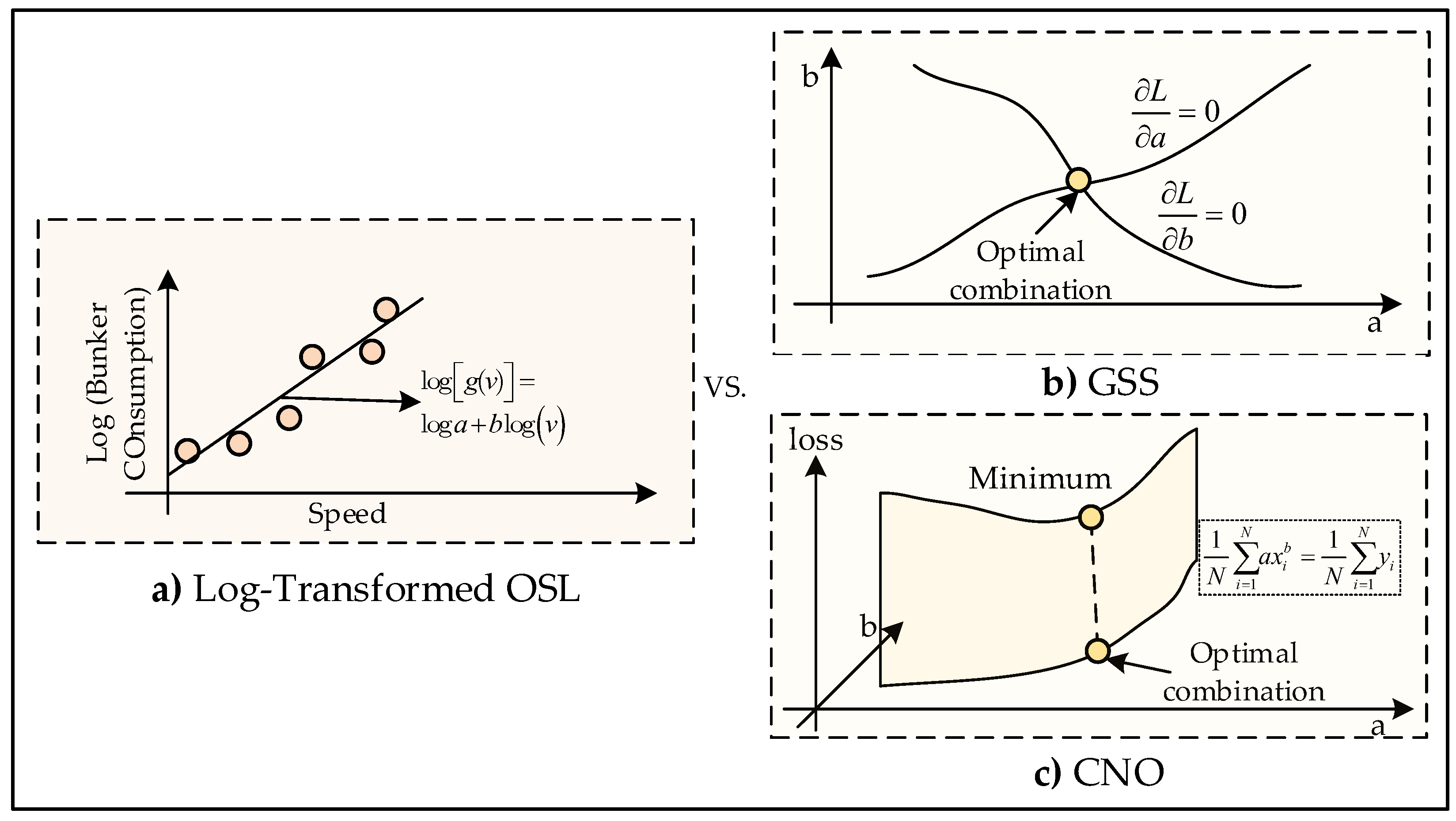
4.2. Direct Estimation Methods

In Section 3.1, we have illustrated the potential limitations of logarithmic transformation. In this section, we will discuss how to optimize the parameters $a$ and $b$ to minimize objective function (15). We let ${\{(x_i,y_i)\}}_{i=1}^N$ be the training data. Then, we solve Model (15) without the nonlinear-to-linear transformation. For a convex problem, an optimal solution can typically be obtained using methods such as gradient descent. Unfortunately, as demonstrated in Proposition 1, objective function (15) is non-convex. Therefore, alternative approaches are required to approximate a near-optimal solution.

Proposition 1. 

Model (15) is non-convex with respect to parameters $a$ and $b$.

Proof. 

Since the model is an unconstrained optimization problem, the convexity of the objective function depends solely on its Hessian matrix. We denote the objective function as

$$L(a,b)={\displaystyle \sum _{i=1}^N{L}_i}(a,b),\hspace{0.33em}\hspace{0.33em}\hspace{0.17em}\mathrm{where}\hspace{0.33em}\hspace{0.33em}\hspace{0.17em}{L}_i(a,b)={(a{x}_i^b-y_i)}^2.$$

(24)

The Hessian matrix of $L(a,b)$ is given by

$$A(L)=\left[\begin{array}{cc}{\displaystyle \frac{{\partial }^{2}L}{\partial a^2}}& {\displaystyle \frac{{\partial }^{2}L}{\partial a\partial b}}\\ {\displaystyle \frac{{\partial }^{2}L}{\partial b\partial a}}& {\displaystyle \frac{{\partial }^{2}L}{\partial b^2}}\end{array}\right]=\left[\begin{array}{cc}{\displaystyle {\displaystyle \sum }_{i=1}^N}2x_i^{2b}& {\displaystyle {\displaystyle \sum }_{i=1}^N}2x_i^b\ln (x_i)(2a{x}_i^b-y_i)\\ {\displaystyle {\displaystyle \sum }_{i=1}^N}2x_i^b\ln (x_i)(2a{x}_i^b-y_i)& {\displaystyle {\displaystyle \sum }_{i=1}^N}2a{x}_i^b{\ln }^2(x_i)(2a{x}_i^b-y_i)\end{array}\right].$$

(25)

The determinant of this Hessian matrix is

$$|A(L)|=\left({\displaystyle \sum }_{i=1}^{N}2x_i^{2b}\right)\cdot \left({\displaystyle \sum }_{i=1}^{N}2a{x}_i^b{\ln }^2(x_i)(2a{x}_i^b-y_i)\right)-{\left({\displaystyle \sum }_{i=1}^{N}2x_i^b\ln (x_i)(2a{x}_i^b-y_i)\right)}^2.$$

(26)

To determine whether the objective function is convex, we examine the determinant of the Hessian matrix. The function $L\left(a, b\right)$ is convex if and only if the Hessian matrix is positive semidefinite. However, we observe from the structure of Formula (26) that the sign of the determinant depends on the term ${\displaystyle \sum _{i=1}^N}2a{x}_i^b{\ln }^2(x_i)(2a{x}_i^b-y_i)$. Specifically, if values of $a$ and $b$ cause this term to be negative, the determinant will be negative, making the Hessian matrix not positive semidefinite. In particular, the determinant of the Hessian will be negative when

$$2a{x}_i^b-y_i\le 0,i\in \{1,\dots ,N\}.$$

(27)

This condition can be satisfied if we choose $a$ and $b$ that satisfy

$$a<{\displaystyle \frac{{\min }_i\left\{y_i\right\}}{{\max }_i\left\{2{x_i}^b\right\}}}.$$

(28)

Once a value of $b$ is chosen, the corresponding feasible range for $a$ is determined. Hence, Equation (28) defines a feasible domain for $a$ and $b$ such that the determinant of the Hessian is negative, indicating that the Hessian is not positive semidefinite and, consequently, the objective function is not convex. □

To solve Model (15), we take the partial derivatives of $L(a,b)$ respect to $a$ and $b$, respectively, and let them be equal to 0. We obtain

$${\displaystyle \frac{2}{N}}{\displaystyle \sum }_{i=1}^N{x}_i^b(a{x}_i^b-y_i)=0,$$

(29)

$${\displaystyle \frac{2}{N}}{\displaystyle \sum }_{i=1}^{N}a(\ln x_i)x_i^b(a{x}_i^b-y_i)=0.$$

(30)

Then, we attempt to solve the system of Equations (29) and (30). According to Equation (29), the relationship of $a$ and $b$ should satisfy

$$a={\displaystyle \frac{{\displaystyle \sum _{i=1}^N}{x}_i^b{y}_i}{{\displaystyle \sum _{i=1}^N}{x}_i^{2b}}}.$$

(31)

Plugging the above result into Equation (30), we have an equation in the unknown $b$, and we can discretize and enumerate $b$ to obtain the approximate optimal solution. Specifically, we ensure a reasonable range of $b$. In SSO, the range of $b$ can be set to $[1,4]$. Then enumerating the possible values of $b$, we obtain the corresponding value of $a$. By evaluating different possible parameter combinations, we can select the optimal parameter combination that approximately approaches the root of Equation (30). This constitutes the gradient substitution search model.

Letting $(a^{*},b^{*})$ be an approximate optimal solution, this solution may be “biased” in the sense that

$${\displaystyle \frac{1}{N}}{\displaystyle \sum }_{i=1}^N{a}^{*}{x}_i^{b^{*}}\ne {\displaystyle \frac{1}{N}}{\displaystyle \sum }_{i=1}^N{y}_i.$$

(32)

Therefore, we propose the following third estimation model:

$$\underset{a,b}{\min }{\displaystyle \frac{1}{N}}{\displaystyle \sum }_{i=1}^N{\left(a{x}_i^b-y_i\right)}^2$$

(33)

subject to

$${\displaystyle \frac{1}{N}}{\displaystyle \sum }_{i=1}^{N}a{x}_i^b={\displaystyle \frac{1}{N}}{\displaystyle \sum }_{i=1}^N{y}_i.$$

(34)

To solve the above model, we can enumerate possible values of $b$, and then $a$ is determined based on Constraint (34). Then we substitute $a$ and $b$ into Function (33) to obtain the optimal parameter combination that minimizes the mean squared error. This is the third estimation model—constrained nonlinear optimization. Figure 3 visualizes the comparison of three fitting methods. Figure 3a shows the points after log transformation and the corresponding fitted curve. Figure 3b presents the intersection point of the two derivative equations. Figure 3c displays the parameter combination point searched within the constrained space that achieves the lowest fitting error.

4.3. Computational Cost Analysis

Assuming the number of observed samples is $N$, the log transformation applied to all samples incurs a time complexity of $\mathcal{O}(N)$, and the OLS fitting also has a complexity of $\mathcal{O}(N)$. Therefore, the overall complexity of log-transformed OLS is $\mathcal{O}(N)$. In contrast, both the GSS and CNO methods proposed in this study require an exhaustive search over a set of candidate values for the exponent parameter $b$. Let $M$ denote the total number of grid points used in this search. For each candidate $b$, the objective function is evaluated with a computational cost of $\mathcal{O}(N)$, leading to an overall complexity of $\mathcal{O}(N\cdot M)$.

Nevertheless, since $M$ is typically chosen as a fixed and moderate constant in practice, the computational complexity of our methods grows only linearly with the sample size $N$. This ensures that our approach remains computationally efficient and scalable.

5. Case Study

To validate the effectiveness and robustness of our proposed estimation methods, we conduct a series of numerical experiments under diverse settings, including well-specified and mis-specified experiments, varying operational conditions, and randomly generated parameters.

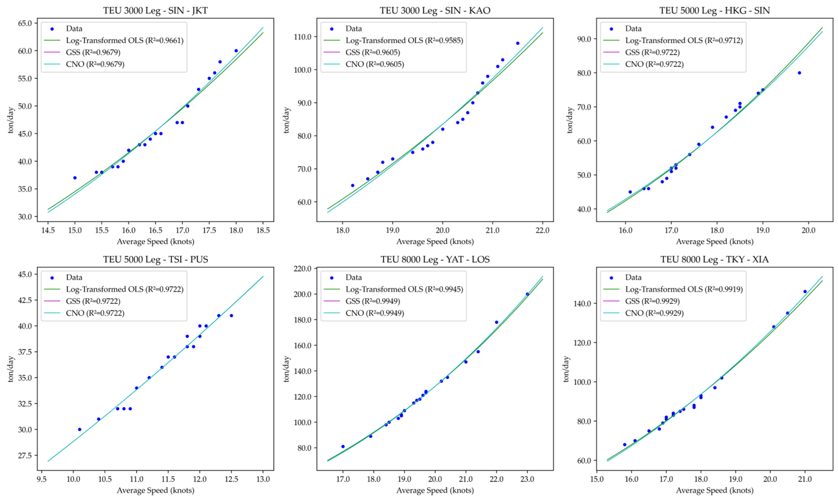
5.1. Estimation Results Using Real-World Data

We use real-world data reported by Wang and Meng [12] to validate the effectiveness of our proposed methods. This dataset provides historical records of average sailing speed (in knots) and bunker fuel consumption (in tons per day) for three types of container ships—3000-TEU, 5000-TEU, and 8000-TEU (where TEU stands for twenty-foot equivalent unit)—across various voyage legs. As shown in Figure 4, both GSS and CNO achieve a higher goodness of fit than log-transformed OLS, as indicated by the value of $R^2$. Moreover, their estimation results are consistently aligned, as evidenced by the near-overlapping curves of GSS and CNO in Figure 4. However, the primary objective of this paper is to reduce the decision-making cost of SSO rather than merely improving the fitting accuracy. Therefore, in the following sections, we will demonstrate how the proposed estimation methods contribute to reducing the bunker consumption.

5.2. Experimental Procedure

The aim of this paper is to reduce the fuel consumption of SSO by providing new methods for estimating parameters $a$ and $b$. We generate the synthetic data with noise following the steps illustrated in Section 4.1, but changing the parameter settings. We first sample a set of data ${\{(x_i,g(x_i))\}}_{i=1}^N$, and then compute the mean $\mu$ of ${\{g(x_i)\}}_{i=1}^N$, and finally generate the training data ${\{(x_i,y_i)\}}_{i=1}^N$ by adding Gaussian white noise with a standard deviation equal to 1% of the $\mu$. Here, $x_i$ represents the observed sailing speed, and $y_i$ denotes the corresponding bunker consumption. We set $N=20$. The specific form and parameters of function $g$ will be reported in the corresponding sections. Then, we adopt three methods, as described above, to estimate the parameters from data with noise and incorporate them into the SSO model, where log-transformed OLS serves as the benchmark. The generated decision is then substituted into objective function (6) using the true parameter settings—that is, the noise-free functional relationship $g$ between sailing speed and bunker consumption. This allows us to obtain the bunker consumption under real parameters, which serves as the evaluation metric.

Additionally, every ship shares the same speed bound at $V_{\min }=10$ (in nautical miles /hour) and $V_{\max }=20$ (in nautical miles/hour). All the experiments in Section 5 follow this speed constraint. Thus, the remaining adjustable parameters ($a_1$, $b_1$, $a_2$, $b_2$, $D$, and $T$) can be assembled into different parameter combinations. $a_1$, $b_1$, $a_2$, and $b_2$ determine the true relationship without noise between speed and bunker consumption. $D$ is the distance between ports $P$ and $Q$. $T$ is the total time window. Below, we will elaborate on how we design our experiments based on adjusting these values and other settings.

Because the synthetic data uses Gaussian noise, which adds randomness to our model, thus, for each parameter combination, we conduct 50 independent repeated experiments with different random seeds. In each experiment, we also assign a rank to each method based on its real bunker consumption.

5.3. Well-Specified and Mis-Specified Experiments

To evaluate the effectiveness of our methods, we first design well-specified and mis-specified experiments. A well-specified experiment refers to the setting where the data-generating process follows the same functional form as the model used for estimation. In contrast, a mis-specified experiment assumes a different data-generating process from the fitted model, introducing a form mismatch. For the well-specified experiment, we assume the true relationship follows the functional form $g(v)=a\cdot v^b$. We conduct six experiments with different parameters, as shown in

Table 3. Parameter setting 1: $g(v)$ as a power function.

No.	${\mathit{a}}_1$	${\mathit{b}}_1$	${\mathit{a}}_2$	${\mathit{b}}_2$	$\mathit{D}$ (Nautical Miles)	$\mathit{T}$ (Hours)
1	0.015	2.90	0.013	3.10	500	60
2	0.010	3.00	0.012	2.80	1600	180
3	0.005	3.10	0.008	3.00	1420	160
4	0.600	1.67	0.550	1.75	480	85
5	0.010	3.20	0.012	3.10	6500	660
6	0.030	2.70	0.025	2.80	1300	150

, which are based on the estimation parameters in Section 5.1.

For the mis-specified setting, we set the true relationship as $g(v)=a\cdot e^{bv}$ rather than the power function form. However, we still use the power function form to fit the generated data and make the decision. The parameter settings can be found in

Table 4. Parameter setting 2: $g(v)$ as an exponential function.

No.	${\mathit{a}}_1$	${\mathit{b}}_1$	${\mathit{a}}_2$	${\mathit{b}}_2$	$\mathit{D}$ (Nautical Miles)	$\mathit{T}$ (Hours)
1	2.24	0.185	2.20	0.190	500	60
2	3.40	0.160	3.60	0.150	1600	180
3	2.55	0.178	2.45	0.180	1420	160
4	6.67	0.148	6.75	0.140	480	85
5	5.70	0.155	5.55	0.160	6500	660
6	6.30	0.150	6.45	0.145	1300	150

.

For the well-specified experiments, we use boxplots to present the results. Avg. rank refers to the average ranks of each method across 50 experiments by changing the random seed. As shown in Figure 5, in all cases, the bunker consumption of our methods is lower on average than that of log-transformed OLS, and their variances are also smaller. Moreover, the results of GSS and CNO, both proposed in this paper, consistently align with each other. These findings demonstrate the robustness and effectiveness of our approaches. However, it is important to note that while our methods lead to some improvement, the extent of this enhancement is modest. This is because, while logarithmic transformation has theoretical limitations, the resulting deviations are usually minimal and do not significantly affect practical engineering applications.

For the mis-specified experiments, the results are shown in Figure 6, in which GSS and CNO consistently achieve higher average rankings compared to the traditional log-transformed OLS. Moreover, their bunker consumptions are always lower than those of log-transformed OLS, with correspondingly smaller variances.

Compared to well-specified experiments, one noteworthy point is that the variances of the results under mis-specified settings are higher than those under well-specified settings. This is because the ground truth in mis-specified settings is generated using an exponential function, while we still fit the data using a power function, which affects the robustness of the decision-making process. Overall, under both well-specified and mis-specified parameter settings, GSS and CNO generally outperform log-transformed OLS.

5.4. Sensitivity Analysis: Voyage Speed and Fuel Consumption Asymmetry

Now, we adjust the parameters to analyze their impacts on the results. We set the real relationship $g$ as a power function, and $a_1=0.01$, $b_1=3$, $a_2=0.012$, $b_2=2.85$, and $T=180$ as constant values. The only variable parameter is $D$, which follows the relationship $D=T\cdot v_{avg}/2$, where $v_{avg}$ are uniformly sampled at equal intervals over the range from 11.5 to 18.5. A total of 50 parameter combinations are generated, corresponding to 50 values of $v_{avg}$ and $D$. These experiments help us to evaluate the influence of average speed on the outcomes. Since the designed average speed $v_{avg}$ directly influences the final decisions $v_1$ and $v_2$, this setup helps to reveal how the fitted function performs across different speed ranges. For the second group of experiments, we set $a_1=0.01$, $b_1=3$, $b_2=3$, $T=180$, and $D=1400$ as constant values. The only altered parameter is $a_2$, ranging from 0.005 to 0.020, corresponding to the round-trip fuel consumption ratio $a_2/a_1$ ranging from 50% to 200%. A total of 50 combinations are generated uniformly, corresponding to 50 values of $a_2$. This setting reflects real-world scenarios where external factors such as wind, current, or loading conditions may cause significant differences in fuel consumption for the two directions.

For these experiments with different parameter settings corresponding to each specific method, we conduct 50 independent runs under different random seeds for each configuration. In each run, we record which of the three methods—GSS, CNO, or log-transformed OLS—leads to the lowest actual fuel consumption after the predicted solution is applied to the optimization problem. We define the “method ratio” as the proportion of runs in which each method achieves the lowest fuel consumption. In the bar chart, each bar corresponds to a specific parameter configuration, and the stacked colors represent the proportion of times each method yields the best actual performance across the 50 runs. The pie chart illustrates the overall proportion of times each method achieves the lowest actual fuel consumption across all experiments, reflecting their general performance advantage under various parameter settings. The boxplot further shows the distribution of these success ratios across configurations, highlighting the stability and robustness of each method.

For experiments varying the average speed, from Figure 7, we observe a clear trend: log-transformed OLS often performs better when the average sailing speed is low. This phenomenon can be partially explained by Figure 2. Specifically, log-transformed OLS achieves better fitting performance when the independent variable $X$ takes smaller values. However, as $X$ increases, the fitting bias of log-transformed OLS becomes more evident, which leads to the performance degradation observed in Figure 7a. In contrast, GSS consistently maintains superior performance across the entire range of average speed, further demonstrating the robustness of the proposed method. We also conduct a statistical analysis of the ratio of best method. From Figure 7b, we observe that in $50\times 50=2500$ experiments, GSS achieved the best performance in 43.1% of the cases, followed by CNO in 34.9%, while the log-transformed OLS accounted for only 22.0%. This observation is further supported by the boxplot in Figure 7c, which shows that the baseline model has the lowest average performance.

For experiments varying the average bunker fuel consumption ratio, in Figure 8, it can be observed that GSS consistently outperforms the others across the entire range of the fuel consumption ratio. Its performance remains stable even when the asymmetry becomes more pronounced, indicating stronger robustness. These results further confirm the effectiveness and stability of GSS in handling complex and uncertain operational environments, especially when cost asymmetry is present. Similarly to Figure 7, Figure 8 leads to comparable conclusions: GSS outperforms CNO, and both methods significantly surpass the baseline model, the log-transformed OLS. Specifically, GSS achieves the best performance in 44.3% of the runs, followed by CNO in 34.9%, while the baseline model accounts for only 20.8%.

5.5. More Diverse Computational Experiments

To further demonstrate the flexibility and robustness of our method, we randomly generate diverse parameter combinations based on the specific rules outlined in

Table 5. Parameter rules.

Parameter	Condition
Interval of $a_1$ and $a_2$	$[0.005,0.05]$
Interval of $b_1$ and $b_2$	$[0.005,0.05]$
Interval of $D$	$[100,\mathrm{10,000}]$
Interval of $T$	$[100,1000]$
Average speed restriction	$[10,20]$
Bunker consumption difference restriction	$0\le {\displaystyle \frac{\left|{\displaystyle {\int }_{10}^{20}{g}_1(v)dv}-{\displaystyle {\int }_{10}^{20}{g}_2(v)dv}\right|}{\max ({\displaystyle {\int }_{10}^{20}{g}_1(v)dv},{\displaystyle {\int }_{10}^{20}{g}_2(v)dv})}}\le 50\%$

. The first four constraints ensure that the parameters remain within a reasonable range, which is achieved using Latin Hypercube Sampling [26]. The fifth constraint is designed to preserve the flexibility of the problem. The final constraint is introduced to ensure that the asymmetry in round-trip fuel consumption remains within a realistic range, thereby aligning with practical operational conditions. We evaluate whether each generated parameter set satisfies conditions five and six—only those that meet both are retained as a candidate parameter combination, while those that fail are discarded. Additionally, the real relationship $g$ is still a power function.

Figure 9 illustrates the results of the method ratios under randomly generated parameter combinations across a large number of experiments. We observe that GSS consistently accounts for a large portion of the method ratio across most parameter combinations, indicating its strong adaptability and robustness in various scenarios. CNO also demonstrates competitive performance, often sharing or exceeding GSS’s success in certain parameter configurations. However, log-transformed OLS appears to dominate in far fewer instances. In Figure 9b,c, although GSS does not have an absolute majority, the overall proportions still indicate that GSS performs better than CNO, with the baseline model log-transformed OLS maintaining the lowest share. The boxplot further shows that the performance of GSS and CNO is similar, with both significantly outperforming the baseline model. This empirical evidence supports the overall conclusion that GSS—and to some extent CNO—exhibit superior generalization capabilities when facing random and potentially challenging parameter combinations, highlighting the advantage of the proposed approaches in real-world applications with high variability and uncertainty.

In summary, the case study comprehensively validates the effectiveness and robustness of the proposed estimation methods across a variety of experimental scenarios. Under controlled parameter settings, varying operational conditions such as average sailing speed and directional fuel consumption asymmetry, or randomly sampled real-world-like configurations, GSS consistently achieves the best performance in approximately 39.1% to 44.3% of the runs, while CNO follows closely with around 34.9% to 35.0%. In contrast, the traditional benchmark log-transformed OLS only leads in 20.8% to 25.9% of the cases. These results demonstrate that both GSS and CNO outperform the baseline method in terms of achieving lower bunker consumption and reduced variance, highlighting their superior accuracy and robustness in complex maritime operational environments.

This further highlights that our model can more accurately capture the functional relationship between fuel consumption and vessel speed, which in turn helps improve the precision of decision-making. Such an enhanced modeling capability allows for the better representation of complex real-world behaviors, ultimately leading to more effective and reliable optimization results compared to baseline approaches. These results not only demonstrate the superior fitting capabilities of our methods, but more importantly, highlight their practical value in supporting more reliable and cost-effective decision-making in real-world shipping operations.

6. Conclusions

This study revisits the challenge of accurately modeling fuel consumption in SSO. Recognizing the limitations of conventional transformation-based regression—particularly issues related to estimation bias and variance instability—we propose two direct fitting methods that operate on the original nonlinear structure of the problem. Empirical evaluations demonstrate that the proposed approach yields more consistent and realistic results, supporting better informed operational decisions. Beyond improving prediction accuracy, our work contributes to bridging the gap between data-driven modeling and practical applicability in maritime transportation.

Despite the encouraging results, this study has several limitations. First, our model focuses on the relationship between sailing speed and fuel consumption under relatively stable operational conditions, without explicitly accounting for dynamic external factors such as weather, sea currents, and cargo load variations. These factors may introduce nonlinearities or temporal dependencies that our current framework does not capture. Second, the proposed methods are validated using historical data from a limited number of vessels; broader generalization across ship types and voyage patterns remains to be tested. In future research, incorporating multi-dimensional features, expanding the model to fleet-level optimization, and integrating the proposed framework into real-time decision-making systems could further enhance its practical value and robustness.

References

1. Yao, Z.; Ng, S.H.; Lee, L.H. A Study on Bunker Fuel Management for the Shipping Liner Services. Comput. Oper. Res. 2012, 39, 1160–1172. [Google Scholar] [CrossRef]
2. Ronen, D. The Effect of Oil Price on the Optimal Speed of Ships. J. Oper. Res. Soc. 1982, 33, 1035–1040. [Google Scholar] [CrossRef]
3. Ronen, D. Ship Scheduling: The Last Decade. Eur. J. Oper. Res. 1993, 71, 325–333. [Google Scholar] [CrossRef]
4. International Maritime Organization. Fourth IMO Greenhouse Gas Study 2020; International Maritime Organization: London, UK, 2020. [Google Scholar]
5. Meng, Q.; Du, Y.; Wang, Y. Shipping Log Data Based Container Ship Fuel Efficiency Modeling. Transp. Res. Part B Methodol. 2016, 83, 207–229. [Google Scholar] [CrossRef]
6. Saki, S.; Soori, M. Artificial Intelligence, Machine Learning and Deep Learning in Advanced Transportation Systems, A Review. Multimodal Transp. 2025, 100242. [Google Scholar] [CrossRef]
7. Coto-Solano, M.E. Demand Study of Freight Transportation via Railway of Four Commodity Groups: A Case Study on Costa Rica’s Pacific Coast Route. Multimodal Transp. 2024, 3, 100157. [Google Scholar] [CrossRef]
8. Vorkapić, A.; Martinčić-Ipšić, S.; Piltaver, R. Interpretable Machine Learning: A Case Study on Predicting Fuel Consumption in VLGC Ship Propulsion. J. Mar. Sci. Eng. 2024, 12, 1849. [Google Scholar] [CrossRef]
9. Liu, Z.; Lyu, C.; Huo, J.; Wang, S.; Chen, J. Gaussian Process Regression for Transportation System Estimation and Prediction Problems: The Deformation and a Hat Kernel. IEEE Trans. Intell. Transp. Syst. 2022, 23, 22331–22342. [Google Scholar] [CrossRef]
10. Fagerholt, K.; Laporte, G.; Norstad, I. Reducing Fuel Emissions by Optimizing Speed on Shipping Routes. J. Oper. Res. Soc. 2010, 61, 523–529. [Google Scholar] [CrossRef]
11. Kim, J.-G.; Kim, H.-J.; Jun, H.B.; Kim, C.-M. Optimizing Ship Speed to Minimize Total Fuel Consumption with Multiple Time Windows. Math. Probl. Eng. 2016, 2016, 3130291. [Google Scholar] [CrossRef]
12. Wang, S.; Meng, Q. Sailing Speed Optimization for Container Ships in a Liner Shipping Network. Transp. Res. Part E Logist. Transp. Rev. 2012, 48, 701–714. [Google Scholar] [CrossRef]
13. Elmachtoub, A.N.; Grigas, P. Smart “Predict, Then Optimize”. Manag. Sci. 2022, 68, 9–26. [Google Scholar] [CrossRef]
14. Donti, P.; Amos, B.; Kolter, J.Z. Task-Based End-to-End Model Learning in Stochastic Optimization. Adv. Neural Inf. Process. Syst. 2017, 30. [Google Scholar] [CrossRef]
15. Ban, G.-Y.; Rudin, C. The Big Data Newsvendor: Practical Insights from Machine Learning. Oper. Res. 2019, 67, 90–108. [Google Scholar] [CrossRef]
16. Yang, L.; Chen, G.; Zhao, J.; Rytter, N.G.M. Ship Speed Optimization Considering Ocean Currents to Enhance Environmental Sustainability in Maritime Shipping. Sustainability 2020, 12, 3649. [Google Scholar] [CrossRef]
17. Lai, X.; Wu, L.; Wang, K.; Wang, F. Robust Ship Fleet Deployment with Shipping Revenue Management. Transp. Res. Part B Methodol. 2022, 161, 169–196. [Google Scholar] [CrossRef]
18. Tarelko, W.; Rudzki, K. Applying Artificial Neural Networks for Modelling Ship Speed and Fuel Consumption. Neural Comput. Appl. 2020, 32, 17379–17395. [Google Scholar] [CrossRef]
19. Du, Y.; Meng, Q.; Wang, S.; Kuang, H. Two-Phase Optimal Solutions for Ship Speed and Trim Optimization over a Voyage Using Voyage Report Data. Transp. Res. Part B Methodol. 2019, 122, 88–114. [Google Scholar] [CrossRef]
20. Le, L.T.; Lee, G.; Park, K.-S.; Kim, H. Neural Network-Based Fuel Consumption Estimation for Container Ships in Korea. Marit. Policy Manag. 2020, 47, 615–632. [Google Scholar] [CrossRef]
21. Yan, R.; Wang, S.; Du, Y. Development of a Two-Stage Ship Fuel Consumption Prediction and Reduction Model for a Dry Bulk Ship. Transp. Res. Part E Logist. Transp. Rev. 2020, 138, 101930. [Google Scholar] [CrossRef]
22. Uyanık, T.; Bakar, N.N.A.; Kalenderli, Ö.; Arslanoğlu, Y.; Guerrero, J.M.; Lashab, A. A Data-Driven Approach for Generator Load Prediction in Shipboard Microgrid: The Chemical Tanker Case Study. Energies 2023, 16, 5092. [Google Scholar] [CrossRef]
23. Shangguan, Y.; Tian, X.; Jin, S.; Gao, K.; Hu, X.; Yi, W.; Guo, Y.; Wang, S. On the Fundamental Diagram for Freeway Traffic: Exploring the Lower Bound of the Fitting Error and Correcting the Generalized Linear Regression Models. Mathematics 2023, 11, 3460. [Google Scholar] [CrossRef]
24. Atkinson, K.E. An Introduction to Numerical Analysis; John Wiley & Sons: New York, NY, USA, 2008. [Google Scholar]
25. Hansen, B. Econometrics; Princeton University Press: Princeton, NJ, USA, 2022. [Google Scholar]
26. McKay, M.D.; Beckman, R.J.; Conover, W.J. A Comparison of Three Methods for Selecting Values of Input Variables in the Analysis of Output from a Computer Code. Technometrics 2000, 42, 55–61. [Google Scholar] [CrossRef]
Figure 1. Overflow of SSO problem and algorithm design. (a) Problem statement of SSO. (b) Algorithm framework for solving SSO problem.
Mathematics 13 01987 g001
Figure 2. An example of limitations of logarithmic transformation. (a) Comparison of fitted and real data; (b) fitted curve and residual after logarithmic transformation; (c) residual in real data; (d) residual in logarithmic space.
Mathematics 13 01987 g002
Figure 3. Comparison of three fitting methods with visualization. (a) Traditional log-transformed OSL method; (b) GSS method; (c) CNO method.
Mathematics 13 01987 g003
Figure 4. Real-world fitting results.
Mathematics 13 01987 g004
Figure 5. Experiment results following well-specified settings.
Mathematics 13 01987 g005
Figure 6. Experiment results following mis-specified settings.
Mathematics 13 01987 g006
Figure 7. Experimental results under varying average sailing speeds: (a) stacked bar chart of method ratios for each parameter setting (with varying random seeds); (b) overall method ratio represented by a pie chart; (c) boxplot of method ratio distributions.
Mathematics 13 01987 g007
Figure 8. Experimental results under varying average bunker fuel consumption ratios a 2 / a 1 : (a) stacked bar chart of method ratios for each parameter setting (with varying random seeds); (b) overall method ratio represented by a pie chart; (c) boxplot of method ratio distributions.
Mathematics 13 01987 g008
Figure 9. Experimental results with random parameters: (a) stacked bar chart of method ratios for each parameter setting (with varying random seeds); (b) overall method ratio represented by a pie chart; (c) boxplot of method ratio distributions.
Mathematics 13 01987 g009