From Lagrange to Bernstein: Generalized Transfinite Elements with Arbitrary Nodes

Abstract

This paper presents a unified framework for constructing transfinite finite elements with arbitrary node distributions, using either Lagrange or Bernstein polynomial bases. Three distinct classes of elements are considered. The first includes elements with structured internal node layouts and arbitrarily positioned boundary nodes. The second comprises elements with internal nodes arranged to allow smooth transitions in a single direction. The third class consists of elements defined on structured T-meshes with selectively omitted internal nodes, resulting in sparsely populated or incomplete grids. For all three classes, new macro-element (global interpolation) formulations are introduced, enabling flexible node configurations. Each formulation supports representations based on either Lagrange or Bernstein polynomials. In the latter case, two alternative Bernstein-based models are developed as follows: one that is numerically equivalent to its Lagrange counterpart, and another that offers modest improvements in numerical performance.

1. Introduction

Computational methods have undergone numerous stages of development and still appear to be evolving. Beginning with the global approaches of Rayleigh [1], followed by those of Ritz [2] and Bubnov–Galerkin (1913–1915), the field gradually transitioned toward local approximation techniques, as exemplified by the finite element method [3,4]. Among these stages of development, transfinite interpolation holds a particularly significant place [5]. Although it was originally introduced with the primary aim of interpolating the geometry of solid objects and surfaces [6], it soon became evident that the methodology could also be employed for interpolating scalar or even vector fields within three-dimensional space. In particular, the transfinite interpolation formula enables the construction of finite elements with differing numbers of nodes on opposite edges or surfaces, without the need for transitional elements. The same principle applies to the merging of dissimilar domains in two or even three dimensions [7].

While transfinite interpolation works perfectly in conjunction with Lagrange polynomials, the same is not the case for Bernstein ones. This is because the former are cardinal polynomials of $[0,1]$-type, in the sense they are interpolatory (take the value of unity) along the stations, whereas the latter are not (take a value less than unity). Nevertheless, both sets hold the partition of unity property. This fact has sustained the conjecture that transfinite interpolation can be extended in such a way that blending functions can be Bernstein polynomials and at the same time they can also be trial functions which interpolate the primary variable U along the stations [8].

Figure 1 presents a compilation of multiple classes of transfinite finite elements.

Recent studies have shown that a direct substitution of Lagrange polynomials with Bernstein polynomials in the final expressions of the shape functions for all types of transfinite elements is feasible and sometimes yields equivalent results for both polynomial sets. To date, this direct replacement—accompanied by a pointwise agreement between the two polynomial families—has been verified for the following four classes of transfinite elements [9]:

• Coons elements (Figure 1a).
• Tensor product elements (Figure 1b).
• Classical transfinite elements of structured pattern (Figure 1c).
• Deformed tensor product elements (Figure 1d).

Moreover, when opposite edges of the patch—where global interpolation is performed—are discretized using different polynomial degrees (e.g., Figure 1e), the straightforward substitution of Lagrange polynomials with Bernstein polynomials (i.e., the direct implementation of the conjecture using Bernstein polynomials as blending functions) results in a different numerical outcome.

In this context, the present work advances the state of the art by investigating arbitrarily noded transfinite elements, in which opposite edges may contain different numbers of nodal points. Beyond the four classes previously mentioned, three additional cases involving distinct structured patterns of internal nodes are also examined as follows:

• Internal nodes in tensor product arrangement (Figure 1e).
• Internal nodes for variable (e.g., gradual) transition (Figure 1f).
• T-mesh (incomplete grid of internal nodes, see Section 5).

The paper is structured as follows. In Section 2, we present the general formulation of transfinite interpolation, using either Lagrange or Bernstein polynomials for representing the blending and trial functions. In Section 3, we present the way in which the transfinite elements are constructed. In Section 4, we present the concept of elimination of the generalized coefficients on the boundary or along horizontal and vertical stations. In Section 5, we present the substitution of constraints into a background tensor product, on which the T-mesh is based. In Section 6, we present the numerical results of all the models, while Section 7 offers a detailed discussion. The paper closes with the conclusions (Section 8) and is followed by six appendices.

2. General Formulation

2.1. State of the Art

The general expression of the transfinite interpolation for 2D-patches is given as follows [5]:

$$\begin{array}{cc}\hfill U(\xi ,\eta )& =P_{\xi }\oplus P_{\eta }\hfill \\ \hfill & =P_{\xi }\left\{U\right\}+P_{\eta }\left\{U\right\}-P_{\xi \eta }\left\{U\right\},\hfill \end{array}$$

(1)

where $P_{\xi }\left\{U\right\}$ and $P_{\eta }\left\{U\right\}$ are the projectors of the quantity U toward $\xi$ and $\eta$ parametric axes, and $P_{\xi \eta }\left\{U\right\}$ is the corrective projector (tensor product of nodal points at the intersections of stations). It is well known that for vertical stations at $\mathsf{\xi }={\xi }_1=0,\dots ,{\xi }_{m+1}=1$, and horizontal stations at $\mathsf{\eta }={\eta }_1=0,\dots ,{\eta }_{n+1}=1$, we construct blending functions $E_i\left(\xi \right)$ and $E_j\left(\eta \right)$ of degree m and n, respectively. Based on the univariate functions $U({\xi }_i,\eta )$ and $U(\xi ,{\eta }_j)$ along the vertical and horizontal stations, respectively, we have the following:

$$\begin{array}{cc}\hfill P_{\xi }\left\{U\right\}& =\sum _{i=1}^{m+1}{E}_i\left(\xi \right)U({\xi }_i,\eta ),\hfill \end{array}$$

(2)

$$\begin{array}{cc}\hfill P_{\eta }\left\{U\right\}& =\sum _{j=1}^{n+1}{E}_j\left(\eta \right)U(\xi ,{\eta }_j),\hfill \end{array}$$

(3)

$$\begin{array}{cc}\hfill P_{\xi \eta }\left\{U\right\}& =\sum _{j=1}^{n+1}\sum _{i=1}^{m+1}{E}_i\left(\xi \right)E_j\left(\eta \right)U({\xi }_i,{\eta }_j).\hfill \end{array}$$

(4)

On the other hand, along each station the variable $U(\xi ,\eta )$ is interpolated in terms of the trial functions, ${\tilde{B}}_i\left(s\right)$, where the variable s represents either of the parameters $(\xi ,\eta )$, as follows:

$$\begin{array}{cc}\hfill \mathrm{Horizontal}\mathrm{station}:U(\xi ,\overline{\eta })& =\sum _{i=1}^{\tilde{m}+1}{\tilde{B}}_i\left(\xi \right)U({\xi }_i,\overline{\eta }),\hfill \end{array}$$

(5)

$$\begin{array}{cc}\hfill \mathrm{Vertical}\mathrm{station}:U(\overline{\xi },\eta )& =\sum _{j=1}^{\tilde{n}+1}{\tilde{B}}_j\left(\eta \right)U(\overline{\xi },{\eta }_j),\hfill \end{array}$$

(6)

where the bar denotes prescribed value of a certain parameter ($\xi$ or $\eta$) along the corresponding station (vertical or horizontal, for $\overline{\xi }$ or $\overline{\eta }$, respectively). In general, the number of nodes ($\tilde{m}+1$ or $\tilde{n}+1$) along a station may be different (less or greater) than the number of stations in the same direction. The case of equality is also included (e.g., in a tensor product).

Henceforth, for the sake of brevity, the symbol $\left\{U\right\}$ after each projector is suppressed, which means that $P_{\xi }\left\{U\right\}$ will be denoted simply as $P_{\xi }$, and so on.

2.2. Extension of the Projectors

The classical interpretation of the well-known projectors ($P_{\xi },P_{\eta },P_{\xi \eta }$) is based on their application to the primary variable $U(\xi ,\eta )$, and this is consistent with the use of Lagrange polynomials as blending functions $E_i\left(\xi \right)$ and $E_j\left(\eta \right)$ [5]. It is well established that Coons interpolation represents a straightforward extension of one-dimensional linear interpolation to two-dimensional domains [8]. Similarly, classical transfinite (Gordon) interpolation generalizes one-dimensional polynomial interpolation to two-dimensional patches. Since one-dimensional polynomial interpolation can be carried out using either Lagrange or Bernstein polynomials, it follows that the classical projectors can likewise be expressed in terms of Bernstein polynomials.

The above claim will be shown for one projector, for example, $P_{\xi }$, and the same holds for the rest of them. Let us consider three points $P_1\left({\xi }_1\right),P_2\left({\xi }_2\right),$ and $P_3\left({\xi }_3\right)$ and the associated values $U_1,U_2,$ and $U_3$ of a univariate function $U\left(\xi \right)$ (Figure 2a). These can be interpolated in terms of the nodal values ($U_1,U_2$, and $U_3$), using the quadratic Lagrange polynomials $E_1\left(\xi \right)=L_{1,2}\left(\xi \right),E_2\left(\xi \right)=L_{2,2}\left(\xi \right)$, and $E_3\left(\xi \right)=L_{3,2}\left(\xi \right)$ as follows:

$$U\left(\xi \right)=E_1\left(\xi \right)U_1+E_2\left(\xi \right)U_2+E_3\left(\xi \right)U_3.$$

(7)

Alternatively, the same points can be interpolated in terms of the generalized coefficients ($a_1,a_2,a_3$) using the quadratic Bernstein polynomials ${\tilde{E}}_1\left(\xi \right)=B_{1,2}\left(\xi \right),{\tilde{E}}_2\left(\xi \right)=B_{2,2}\left(\xi \right)$, and ${\tilde{E}}_3\left(\xi \right)=B_{3,2}\left(\xi \right)$:

$$U\left(\xi \right)={\tilde{E}}_1\left(\xi \right)a_1+{\tilde{E}}_2\left(\xi \right)a_2+{\tilde{E}}_3\left(\xi \right)a_3.$$

(8)

The above univariate equations can be extended from 1D to 2D, and this is implemented first considering the projector $P_{\xi }$ in which the nodal values ($U_1,U_2,U_3$) have been substituted by univariate functions ($U_1\left(\eta \right),U_2\left(\eta \right),U_3\left(\eta \right)$), as shown in Figure 2b, as follows:

$$P_{\xi }\left\{U\right\}=E_1\left(\xi \right)U_1\left(\eta \right)+E_2\left(\xi \right)U_2\left(\eta \right)+E_3\left(\xi \right)U_3\left(\eta \right).$$

(9)

Similarly, in terms of Bernstein polynomials, the same projector is written as

$$P_{\xi }\left\{a\right\}={\tilde{E}}_1\left(\xi \right)a_1\left(\eta \right)+{\tilde{E}}_2\left(\xi \right)a_2\left(\eta \right)+{\tilde{E}}_3\left(\xi \right)a_3\left(\eta \right).$$

(10)

Of course, there is a significant difference between the above two formulations. Lagrange interpolation (Equation (9)) is local and refers to univariate functions representing the true variable $U\left(\eta \right)$ along stations (at $\xi =0,{\displaystyle \frac{1}{2}},1$), whereas Bernstein interpolation (Equation (10)) is global and refers to univariate functions $a\left(\eta \right)$ made of generalized coefficients. This means that while the interpolation of the primary variable U is obvious, the analogous interpolation of the coefficient a is not. On the other hand, the coefficient a represents an affirmative entity which does not differ from the variable U. For example, in quadratic interpolation we have the following:

$$a_1=U_1,a_2=-{\displaystyle \frac{1}{2}}{U}_1+2U_2+{\displaystyle \frac{1}{2}}{U}_3,a_3=U_3.$$

(11)

Therefore, if, for example, the extreme values are equal (i.e., $U_1=U_3$), the variable $a_2$ represents $2U_2$. This, in turn, means that a doublication of the associated basis function may control $a_2$ and represent the actual variable $U_2$.

Numerical results have demonstrated that the above concept—advocating the use of Bernstein polynomials, and more generally B-splines, as blending functions—performs effectively, provided that the remaining two projectors ($P_{\xi },P_{\eta }$) are also taken into account [8].

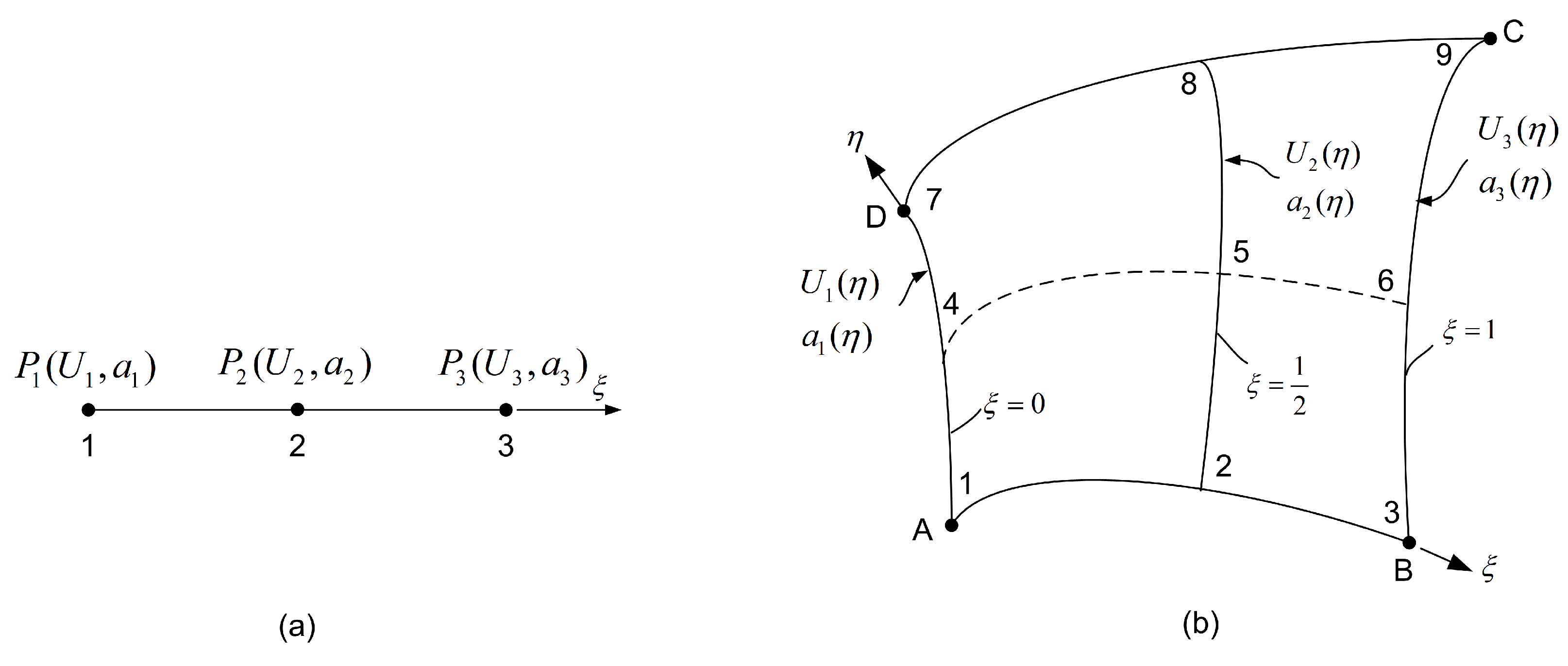
3. Construction of Transfinite Elements

If the univariate functions U given by Equations (5) and (6) are substituted in the three projectors (Equation (2)–(4)), and the latter is substituted into the transfinite interpolation formula given by Equation (1), factoring out this expression gives the global bivariate shape functions ${\varphi }_k(\xi ,\eta )$, so that the primary variable $U(\xi ,\eta )$ is written as follows:

$$U(\xi ,\eta )=\sum _{k=1}^n{\varphi }_k(\xi ,\eta )U_k,$$

(12)

where n is the total number of nodal points (degrees of freedom: DOFs).

In general, arbitrary-noded elements are usually constructed using all the three projectors involved in the transfinite interpolation formula given by Equation (1). However, in some cases, this expression may be simplified, as shown in Section 3.1 and Section 3.2. The golden rule for this simplification is usually one of the following two cases:

• If a nodal point lies on the boundary but neither coincides with any of the four patch corners nor corresponds to an intersection between the boundary and another orthogonal station, then only one of the three associated projections remains active.
• If the nodal point lies at the intersection of two stations, and at least one of them shares the same discretization as the blending functions, then only one projection operator remains active.

Next, by means of an illustrative example concerning a relatively small element, we present the process of shape function derivation and their subsequent implementation using Lagrange and Bernstein polynomial bases.

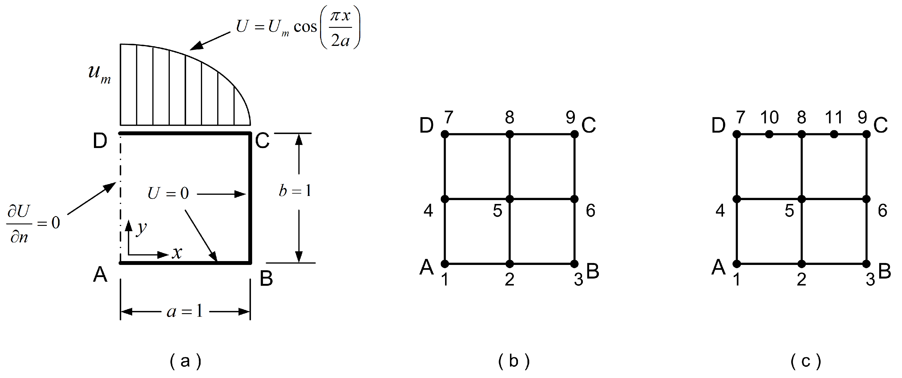
3.1. Tensor Product 9-Node Element

Let us consider the tensor product biquadratic (9-node) element shown in Figure 3a. Considering the linear relationship between univariate Lagrange and Bernstein–Bézier polynomials, it has been previously shown that this conventional element of Lagrange type is mathematically equivalent to the biquadratic tensor product Bézier element [7]. This means that there is a transformation matrix $\mathbf{R}$ of size ($9\times 9$), which relates the nine bivariate shape functions ${\varphi }_i(\xi ,\eta )$ of the former with the nine bivariate basis functions ${\psi }_i(\xi ,\eta )$ of the latter, through the relationship $\mathsf{\varphi }=\mathbf{R}\mathsf{\psi }$. Therefore, although the stiffness matrices (${\mathbf{K}}_L$ and ${\mathbf{K}}_B$) are not identical (one is a quadratic form of the other, e.g., ${\mathbf{K}}_L=\mathbf{R}{\mathbf{K}}_B{\mathbf{R}}^T$), the numerical solutions become identical in both boundary-value and eigenvalue problems.

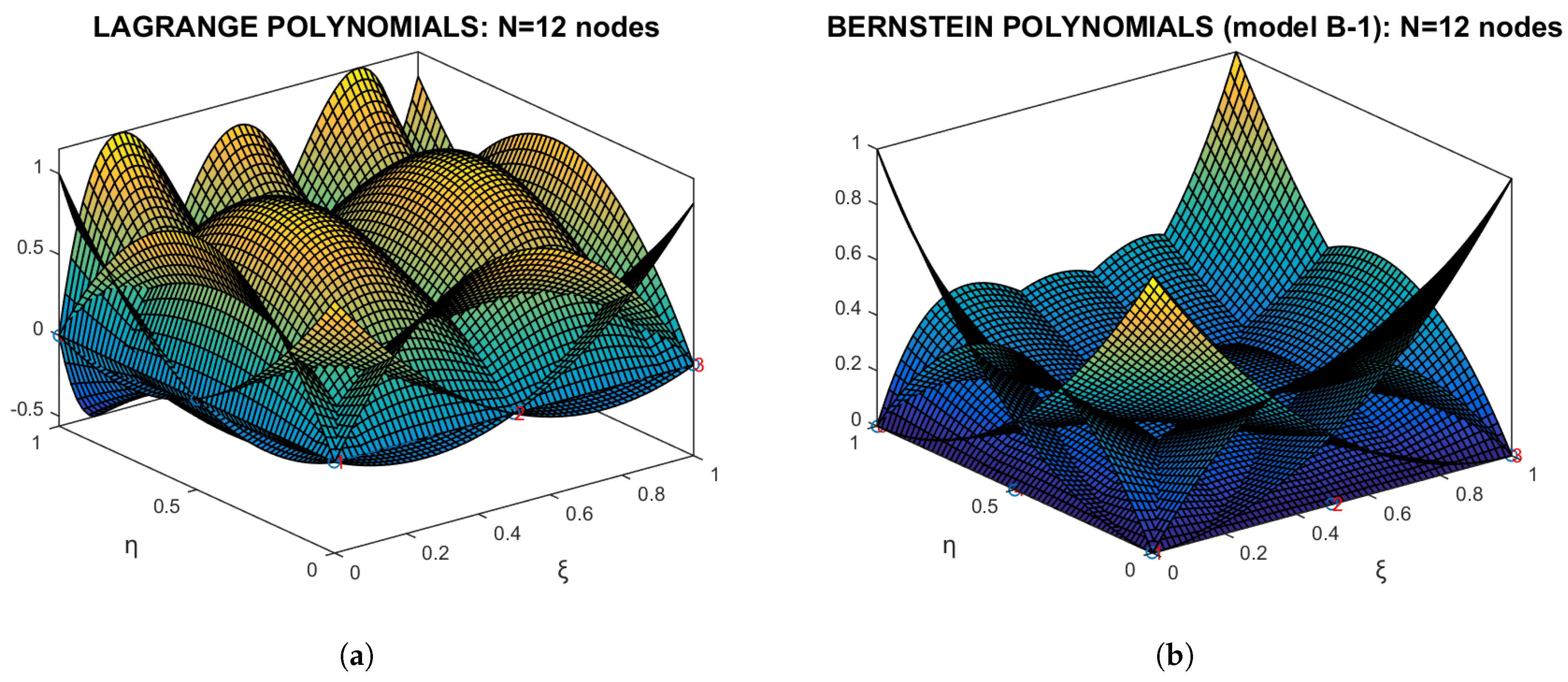
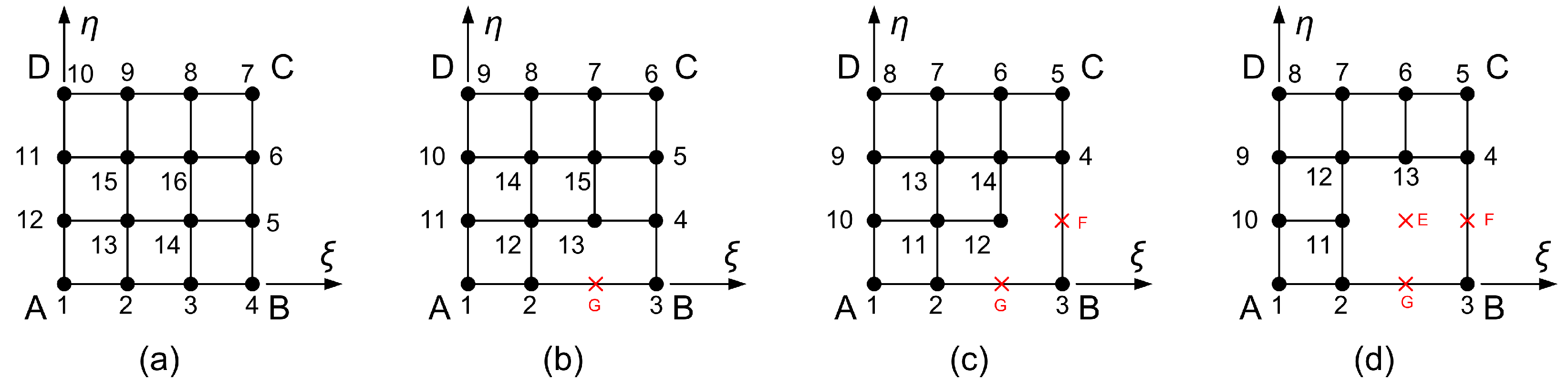
3.2. Transfinite 11-Node Element Described by Only One Projector

Let us continue with the above 9-node tensor product bi-quadratic element shown in Figure 3a. This can be also considered as a transfinite element, which is characterized by three vertical stations (at $\xi =0,{\displaystyle \frac{1}{2}},1$) and three horizontal stations (at $\eta =0,{\displaystyle \frac{1}{2}},1$). Let us also focus on the top edge $DC$, on which two nodes (numbered as 10 and 11) are added, as illustrated in Figure 3b. Obviously, this refinement does not influence the number and location of the stations, which remain the same. In both cases (9-node and 11-node element), the projectors $P_{\xi }$ and $P_{\xi \eta }$ are the same and are written as follows:

$$\begin{array}{cc}\hfill P_{\xi }(\xi ,\eta )& =E_1\left(\xi \right)\left[L_{1,2}\left(\eta \right)U_1+L_{2,2}\left(\eta \right)U_4+L_{3,2}\left(\eta \right)U_7\right]\hfill \\ \hfill & +E_2\left(\xi \right)\left[L_{1,2}\left(\eta \right)U_2+L_{2,2}\left(\eta \right)U_5+L_{3,2}\left(\eta \right)U_8\right]\hfill \\ \hfill & +E_3\left(\xi \right)\left[L_{1,2}\left(\eta \right)U_3+L_{2,2}\left(\eta \right)U_6+L_{3,2}\left(\eta \right)U_9\right],\hfill \end{array}$$

(13)

$$\begin{array}{cc}\hfill P_{\xi \eta }(\xi ,\eta )& =\left[E_1\left(\xi \right)E_1\left(\eta \right)\right]U_1+\left[E_2\left(\xi \right)E_1\left(\eta \right)\right]U_2+\left[E_3\left(\xi \right)E_1\left(\eta \right)\right]U_3\hfill \\ \hfill & +\left[E_1\left(\xi \right)E_2\left(\eta \right)\right]U_4+\left[E_2\left(\xi \right)E_2\left(\eta \right)\right]U_5+\left[E_3\left(\xi \right)E_2\left(\eta \right)\right]U_6\hfill \\ \hfill & +\left[E_1\left(\xi \right)E_3\left(\eta \right)\right]U_7+\left[E_2\left(\xi \right)E_3\left(\eta \right)\right]U_8+\left[E_3\left(\xi \right)E_3\left(\eta \right)\right]U_9.\hfill \end{array}$$

(14)

The symbol $L_{i,j}$ denotes the i-th Lagrange polynomial of degree j.

Since there are three stations per direction, this implies that the blending functions $(E_1,E_2,E_3)$ will be quadratic Lagrange polynomials. Moreover, since there are three nodal points along the vertical stations, the first being on $AD$ (with nodal points: 1-4-7), the second defined by the nodes 2-5-8, and the third on edge $BC$ (with nodal points: 3-6-9), the trial functions will be quadratic polynomials as well. Therefore we have the following:

$$E_1\left(s\right)=L_{1,2}\left(s\right),E_2\left(s\right)=L_{2,2}\left(s\right),E_3\left(s\right)=L_{3,2}\left(s\right),$$

(15)

where the variable s represents either of the parameters $\xi$ or $\eta$.

Substituting Equation (15) into Equations (13) and (14), one may observe that

$$P_{\xi }=P_{\xi \eta }.$$

(16)

Further substitution of Equation (16) into Equation (1) leads to the following:

$$U(\xi ,\eta )=P_{\eta }.$$

(17)

Equation (17) typically arises when all nodal points are positioned along lines parallel to the $\xi$-axis and thus perpendicular to the $\eta$-axis. This geometric arrangement simplifies the subsequent discussion of the 11-node element, which is analyzed using either Lagrange polynomials (Section 3.3) or Bernstein polynomials (Section 3.4).

3.3. Element Formulation Based on Lagrange Polynomials

As previously mentioned, the utilization of Lagrange polynomials, for both the blending functions $E_i=L_{i,2},i=1,2,3$ and the trial functions ${\tilde{B}}_j=L_{j,2},j=1,2,3$, makes handling transfinite interpolation easy. For example, whether the discretization along the top edge $DC$ is (symmetric or not), the dominating projector $P_{\eta }$—which describes the entire $U(\xi ,\eta )$—can be written in terms of the three horizontal isolines, as follows:

$$\begin{array}{cc}\hfill P_{\eta }& =\left[\begin{array}{ccc}{E}_1\left(\eta \right)& E_2\left(\eta \right)& E_3\left(\eta \right)\end{array}\right]\left[\begin{array}{c}U{\left(\xi \right)}_{(\eta =0)}\\ U{\left(\xi \right)}_{(\eta ={\displaystyle \frac{1}{2}})}\\ U{\left(\xi \right)}_{(\eta =1)}\end{array}\right].\hfill \end{array}$$

(18)

The advantage of this expression (compared to intuitive methods cited in textbooks [3,4]) is that any discretization may be chosen along the edge $DC$, which is described by the univariate function $U{\left(\xi \right)}_{(\eta =1)}$. For example, if two nodes (i.e., those numbered as 10 and 11 in Figure 3a) are added to the tensor product, the totality of univariate functions involved in the utmost right end of Equation (18) will be written as follows:

$$\begin{array}{cc}\hfill U{\left(\xi \right)}_{(\eta =0)}& =L_{1,2}\left(\xi \right)U_1+L_{2,2}\left(\xi \right)U_2+L_{3,2}\left(\xi \right)U_3,\hfill \end{array}$$

(19)

$$\begin{array}{cc}\hfill U{\left(\xi \right)}_{(\eta ={\displaystyle \frac{1}{2}})}& =L_{1,2}\left(\xi \right)U_4+L_{2,2}\left(\xi \right)U_5+L_{3,2}\left(\xi \right)U_6,\hfill \end{array}$$

(20)

$$\begin{array}{cc}\hfill U{\left(\xi \right)}_{(\eta =1)}& =L_{1,4}\left(\xi \right)U_7+L_{2,4}\left(\xi \right)U_{10}+L_{3,4}\left(\xi \right)U_8+L_{4,4}\left(\xi \right)U_{11}+L_{5,4}\left(\xi \right)U_9.\hfill \end{array}$$

(21)

Substituting Equations (19)–(21) into Equation (18), and also considering Equation (17), one obtains the following set of global shape functions:

$$\begin{array}{cc}\hfill {\varphi }_1(\xi ,\eta )& =L_{1,2}\left(\xi \right)E_1\left(\eta \right),\hfill \\ \hfill {\varphi }_2(\xi ,\eta )& =L_{2,2}\left(\xi \right)E_1\left(\eta \right),\hfill \\ \hfill {\varphi }_3(\xi ,\eta )& =L_{3,2}\left(\xi \right)E_1\left(\eta \right),\hfill \\ \hfill {\varphi }_4(\xi ,\eta )& =L_{1,2}\left(\xi \right)E_2\left(\eta \right),\hfill \\ \hfill {\varphi }_5(\xi ,\eta )& =L_{2,2}\left(\xi \right)E_2\left(\eta \right),\hfill \\ \hfill {\varphi }_6(\xi ,\eta )& =L_{3,2}\left(\xi \right)E_2\left(\eta \right),\hfill \\ \hfill {\varphi }_7(\xi ,\eta )& =L_{1,4}\left(\xi \right)E_3\left(\eta \right),\hfill \\ \hfill {\varphi }_8(\xi ,\eta )& =L_{3,4}\left(\xi \right)E_3\left(\eta \right),\hfill \\ \hfill {\varphi }_9(\xi ,\eta )& =L_{5,4}\left(\xi \right)E_3\left(\eta \right),\hfill \\ \hfill {\varphi }_{10}(\xi ,\eta )& =L_{2,4}\left(\xi \right)E_3\left(\eta \right),\hfill \\ \hfill {\varphi }_{11}(\xi ,\eta )& =L_{4,4}\left(\xi \right)E_3\left(\eta \right).\hfill \end{array}$$

(22)

We recall that $E_i\left(\eta \right),i=1,2,3$ are quadratic Lagrange polynomials, and that $L_{j,2}\left(\xi \right)$ are also quadratic polynomials, satisfying $L_{j,2}\left(\xi \right)\equiv E_j\left(\xi \right)$, while $L_{j,4}\left(\xi \right)$ are quartic polynomials (degree $p=4$). Although $L_{j,2}$ and $E_j$ represent the same functions, distinct notations are used in Equation (22) to enhance clarity. The set of eleven shape functions is depicted in Figure 4a.

It can be observed that all shape functions are local tensor products of the blending functions $E_i\left(\eta \right)$ associated with the i-th horizontal station and the Lagrange polynomial $L_j\left(\xi \right)$, identified by their serial number j at the current station. Each of the two lower stations is associated with three Lagrange polynomials, whereas the third (top) station is associated with five. In other words, the increase in the number of nodes along an edge (relative to the number of stations) does not significantly affect the formulation.

3.4. Element Formulation Based on Bernstein Polynomials

For a given degree n, a series of $n+1$ Bernstein polynomials is defined as follows:

$$B_{i,n}\left(\xi \right)={\displaystyle \frac{n!}{(i-1)!(n-i+1)!}}{\xi }^{i-1}{(1-\xi )}^{n-i+1},i=1,\dots ,n+1.$$

(23)

In a previous report [8], it was conjectured that the Lagrange polynomials, used in the expression of global shape functions for transfinite elements, could be blindly substituted with Bernstein polynomials of the same degree. Ongoing research has confirmed that this substitution is entirely valid when applied to tensor product elements (ideal or distorted), as well as to non-tensor product classical structured elements in which the same number of nodes exists along every set of parallel stations [9].

However, in cases where a different discretization is present along at least one set of parallel stations—such as along the top edge $DC$ illustrated in Figure 3b, where five nodes are placed, in contrast to only three nodes on the others—a small discrepancy was observed between the two models. Details on two possible models are provided below in Section 3.4.1 and Section 3.4.2.

3.4.1. First Approach (Model B-1): Straight Forward (Blind) Replacement

The theoretical foundation of this approach lies in the application of transfinite interpolation, now employing Bernstein polynomials instead of Lagrange polynomials for both blending and trial functions. However, this choice has the characteristic that the blending functions do not take unity or zero values at internal stations; nonetheless, they retain the partition of unity property. For the 11-node element, where only the projector $P_{\eta }$ is active, the conjecture of Bernstein-based blending functions leads to the following reconstruction of Equation (18):

$$\begin{array}{cc}\hfill P_{\eta }& =\left[\begin{array}{ccc}{B}_{1,2}\left(\eta \right)& B_{2,2}\left(\eta \right)& B_{3,2}\left(\eta \right)\end{array}\right]\left[\begin{array}{c}U{\left(\xi \right)}_{(\eta =0)}\\ \tilde{a}{\left(\xi \right)}_{(\eta ={\displaystyle \frac{1}{2}})}\\ U{\left(\xi \right)}_{(\eta =1)}\end{array}\right].\hfill \end{array}$$

(24)

Clearly, while $U{\left(\xi \right)}_{(\eta =0)}$ and $U{\left(\xi \right)}_{(\eta =1)}$ correspond to the primary variable on the edges $AB$ and $DC$, respectively, the nature of function $\tilde{a}{\left(\xi \right)}_{(\eta ={\displaystyle \frac{1}{2}})}$ remains unspecified (i.e., it is influenced by all eleven $U_i$’s). Nevertheless, this flexibility implies that the univariate functions along the boundary can be defined arbitrarily. For instance, the blending functions $B_{1,2}\left(\eta \right)$ and $B_{2,2}\left(\eta \right)$ have no influence on the edge $DC$, on which $U{\left(\xi \right)}_{(\eta =1)}$ is active. In this context, a reasonable choice is to interpolate $U{\left(\xi \right)}_{(\eta =1)}$ using Bernstein polynomials as follows:

$$U{\left(\xi \right)}_{(\eta =1)}=B_{1,4}\left(\xi \right)a_7+B_{2,4}\left(\xi \right)a_{10}+B_{3,4}\left(\xi \right)a_8+B_{4,4}\left(\xi \right)a_{11}+B_{5,4}\left(\xi \right)a_9.$$

(25)

A more rigorous approach involves starting with the tensor product of Bernstein polynomials, which is mathematically equivalent to the tensor product of Lagrange polynomials of the same degree [8]. In this context, for the 9-node element Equation (24), it becomes as follows:

$$\begin{array}{cc}\hfill U(\xi ,\eta )& =B_{1,2}\left(\eta \right)\underset{U{\left(\xi \right)}_{(\eta =0)}}{\underbrace{\left[B_{1,2}\left(\xi \right)a_1+B_{2,2}\left(\xi \right)a_2+B_{3,2}\left(\xi \right)a_3\right]}}\hfill \\ \hfill & +B_{2,2}\left(\eta \right)\underset{\tilde{a}{\left(\xi \right)}_{(\eta =1/2)}}{\underbrace{\left[B_{1,2}\left(\xi \right)a_4+B_{2,2}\left(\xi \right)a_5+B_{3,2}\left(\xi \right)a_6\right]}}\hfill \\ \hfill & +B_{3,2}\left(\eta \right)\underset{U{\left(\xi \right)}_{(\eta =1)}}{\underbrace{\left[B_{1,2}\left(\xi \right)a_7+B_{2,2}\left(\xi \right)a_8+B_{3,2}\left(\xi \right)a_9\right]}}.\hfill \end{array}$$

(26)

As observed in Equation (26), the univariate function $U\left(\xi \right)$ evaluated at $\eta =1$, corresponding to the edge $DC$, is associated with the blending function $B_{3,2}\left(\eta \right)$. Equation  (26) refers to a 9-node element. To update to the 11-node element, it is only required to modify the aforementioned univariate function $U\left(\xi \right)$ evaluated at $\eta =1$ using the following approximation:

$$\begin{array}{cc}\hfill U{\left(\xi \right)}_{(\eta =1)}& =B_{1,4}\left(\xi \right)a_7+B_{2,4}\left(\xi \right)a_{10}+B_{3,4}\left(\xi \right)a_8+B_{4,4}\left(\xi \right)a_{11}+B_{5,4}\left(\xi \right)a_9.\hfill \end{array}$$

(27)

Substituting Equation (27) into the third term of Equation (26), we receive the following:

$$\begin{array}{cc}\hfill U(\xi ,\eta )& =B_{1,2}\left(\eta \right)\left[B_{1,2}\left(\xi \right)a_1+B_{2,2}\left(\xi \right)a_2+B_{3,2}\left(\xi \right)a_3\right]\hfill \\ \hfill & +B_{2,2}\left(\eta \right)\left[B_{1,2}\left(\xi \right)a_4+B_{2,2}\left(\xi \right)a_5+B_{3,2}\left(\xi \right)a_6\right]\hfill \\ \hfill & +B_{3,2}\left(\eta \right)\left[B_{1,4}\left(\xi \right)a_7+B_{2,4}\left(\xi \right)a_{10}+B_{3,4}\left(\xi \right)a_8+B_{4,4}\left(\xi \right)a_{11}+B_{5,4}\left(\xi \right)a_9\right],\hfill \end{array}$$

(28)

and therefore the set of eleven basis functions for model B-1 will be as follows:

$$\begin{array}{cc}\hfill {\psi }_1(\xi ,\eta )& =B_{1,2}\left(\xi \right)B_{1,2}\left(\eta \right),\hfill \\ \hfill {\psi }_2(\xi ,\eta )& =B_{2,2}\left(\xi \right)B_{1,2}\left(\eta \right),\hfill \\ \hfill {\psi }_3(\xi ,\eta )& =B_{3,2}\left(\xi \right)B_{1,2}\left(\eta \right),\hfill \\ \hfill {\psi }_4(\xi ,\eta )& =B_{1,2}\left(\xi \right)B_{2,2}\left(\eta \right),\hfill \\ \hfill {\psi }_5(\xi ,\eta )& =B_{2,2}\left(\xi \right)B_{2,2}\left(\eta \right),\hfill \\ \hfill {\psi }_6(\xi ,\eta )& =B_{3,2}\left(\xi \right)B_{2,2}\left(\eta \right),\hfill \\ \hfill {\psi }_7(\xi ,\eta )& =B_{1,4}\left(\xi \right)B_{3,2}\left(\eta \right),\hfill \\ \hfill {\psi }_8(\xi ,\eta )& =B_{3,4}\left(\xi \right)B_{3,2}\left(\eta \right),\hfill \\ \hfill {\psi }_9(\xi ,\eta )& =B_{5,4}\left(\xi \right)B_{3,2}\left(\eta \right),\hfill \\ \hfill {\psi }_{10}(\xi ,\eta )& =B_{2,4}\left(\xi \right)B_{3,2}\left(\eta \right),\hfill \\ \hfill {\psi }_{11}(\xi ,\eta )& =B_{4,4}\left(\xi \right)B_{3,2}\left(\eta \right).\hfill \end{array}$$

(29)

The set of basis functions described by Equation (29) is illustrated in Figure 4b, where one may observe that it consists of only non-negative entries.

Within the patch $ABCD$, the primary variable $U(\xi ,\eta )$ is interpolated by the following:

$$U(\xi ,\eta )=\sum _{j=1}^{11}{\psi }_j(\xi ,\eta )a_j.$$

(30)

We recall that the univariate functions involved in Equation (29) are blind (straight forward) replacements of the polynomials used in Equation (22). As previously mentioned, the following hold:

• The functions $E_j\left(\eta \right),j=1,2,3$ are quadratic (degree $p=2$) and thus will be blindly substituted by the following three quadratic Bernstein polynomials: $B_{1,2}\left(\eta \right),B_{2,2}\left(\eta \right),$ and $B_{3,2}\left(\eta \right)$.
• The functions $L_{i,2}\left(\xi \right),i=1,2,3$ are quadratic and thus will be blindly substituted by the following three quadratic Bernstein polynomials: $B_{1,2}\left(\xi \right),B_{2,2}\left(\xi \right)$, and $B_{3,2}\left(\xi \right)$.
• The functions $L_{i,4}\left(\xi \right),i=1,2,3,4,5$ are quartic (degree $p=4$) and thus will be blindly substituted by the following five quartic Bernstein polynomials: $B_{1,4}\left(\xi \right),B_{2,4}\left(\xi \right),B_{3,4}\left(\xi \right),B_{4,4}\left(\xi \right)$, and $B_{5,4}\left(\xi \right)$.

Remark 1. 

The direct substitution of Lagrange polynomials with Bernstein polynomials of the same degree is based on the conjecture that both blending and trial functions can also be expressed using Bernstein polynomials [8].

3.4.2. Second Approach (Model B-2): Accurate Process of Transfinite Interpolation Formula

As we will see later on Section 6.1, model B-1 described by the set of Equation (29)—based on Bernstein polynomials—does not lead to the same numerical solution as that of Equation (22) (based on Lagrange polynomials). This fact can be accomplished by starting from Equation (22) and substituting the Lagrange polynomials (operating as blending and trial functions) with equivalent Bernstein polynomials. Details are provided below.

It is well known that quadratic Lagrange polynomials ($L_{i,2}\left(\eta \right),i=1,2,3$)—stored in column vector $\mathbf{L}\left(\eta \right)$—are connected to quadratic Bernstein polynomials ($B_{i,2}\left(\eta \right),i=1,2,3$)—stored in column vector $\mathbf{B}\left(\eta \right)$—through a transformation matrix ${\mathbf{T}}_2$, which fulfills the following linear relationship:

$$\begin{array}{cc}\hfill {\mathbf{E}}_{\eta }& =\left[\begin{array}{c}{E}_1\left(\eta \right)\\ E_2\left(\eta \right)\\ E_3\left(\eta \right)\end{array}\right]=\underset{\mathbf{L}\left(\eta \right)}{\underbrace{\left[\begin{array}{c}{L}_{1,2}\left(\eta \right)\\ L_{2,2}\left(\eta \right)\\ L_{3,2}\left(\eta \right)\end{array}\right]}}=\underset{{\mathbf{T}}_2}{\underbrace{\left[\begin{array}{ccc}1& -1/2& 0\\ 0& 2& 0\\ 0& -1/2& 1\end{array}\right]}}\underset{\mathbf{B}\left(\eta \right)}{\underbrace{\left[\begin{array}{c}{B}_{1,2}\left(\eta \right)\\ B_{2,2}\left(\eta \right)\\ B_{3,2}\left(\eta \right)\end{array}\right]}}.\hfill \end{array}$$

(31)

Therefore, we have the following:

$$\begin{array}{cc}{E}_1\left(\eta \right)\hfill & =L_{1,2}\left(\eta \right)=B_{1,2}\left(\eta \right)-\frac{1}{2}{B}_{2,2}\left(\eta \right),\hfill \end{array}$$

(32)

$$\begin{array}{cc}{E}_2\left(\eta \right)\hfill & =L_{2,2}\left(\eta \right)=2B_{2,2}\left(\eta \right),\hfill \end{array}$$

(33)

$$\begin{array}{cc}{E}_3\left(\eta \right)\hfill & =L_{3,2}\left(\eta \right)=-\frac{1}{2}{B}_{2,2}\left(\eta \right)+B_{3,2}\left(\eta \right).\hfill \end{array}$$

(34)

If we mechanically substitute Equations (32) through (34) into Equation (22), we once again obtain the same set of cardinal shape functions as those derived using Lagrange polynomials (of the [0,1]-type), but now expressed in terms of Bernstein polynomials. This set, still associated with the $U_i$’s, would again be illustrated in Figure 4a. However, this formulation is not meaningful.

A more meaningful procedure is to recall Equation (18) and substitute the therein univariate functions in terms of Bernstein polynomials. In this context, the first function, $U{\left(\xi \right)}_{(\eta =0)}$, is now expressed in terms of Bernstein polynomials (instead of the Lagrange polynomials involved in Equation (19), etc.), as follows:

$$\begin{array}{cc}U{\left(\xi \right)}_{(\eta =0)}\hfill & =B_{1,2}\left(\xi \right)a_1+B_{2,2}\left(\xi \right)a_2+B_{3,2}\left(\xi \right)a_3,\hfill \end{array}$$

(35)

$$\begin{array}{cc}U{\left(\xi \right)}_{(\eta ={\displaystyle \frac{1}{2}})}\hfill & =L_{1,2}\left(\xi \right)U_4+L_{2,2}\left(\xi \right)U_5+L_{3,2}\left(\xi \right)U_6,\hfill \end{array}$$

(36)

$$\begin{array}{cc}U{\left(\xi \right)}_{(\eta =1)}\hfill & =B_{1,4}\left(\xi \right)a_7+B_{2,4}\left(\xi \right)a_{10}+B_{3,4}\left(\xi \right)a_8+B_{4,4}\left(\xi \right)a_{11}+B_{5,4}\left(\xi \right)a_9.\hfill \end{array}$$

(37)

It is worthy to note that, on the bottom edge ($\eta =0$, Equation (35)) and top edge ($\eta =1$, Equation (37)), we have substituted the Lagrange polynomials by Bernstein polynomials. Furthermore, the nodal variables $U_i$ have been substituted by coefficients $a_i$. This happens because interpolation on edges is independent of the rest domain and is thus univariate (see Appendix A). In contrast, in the middle horizontal station ($\eta =1/2$), the associated nodes 4-5-6 do not still allow for direct interpolation through Bernstein polynomials, simply because the ends are not related with interpolating functions equal to unity. Therefore, we have temporarily preserved the initial formulation given by Equation (36).

Therefore, regarding Equation (36), we proceed as follows:

• First, the three Lagrange polynomials, i.e., $L_{1,2}\left(\xi \right),L_{2,2}\left(\xi \right),$ and $L_{3,2}\left(\xi \right)$, which are involved in Equation (36), are replaced in terms of the Bernstein polynomials, using Equations (32)–(34).
• Moreover, the extreme nodal values are expressed in terms of the boundary coefficients, considering the transpose inverse of Equation (31) (see also Appendix A), i.e.,

  $$\begin{array}{c}\hfill \left[\begin{array}{c}{U}_1\\ U_4\\ U_7\end{array}\right]=\underset{{\left({\mathbf{T}}_2^T\right)}^{-1}}{\underbrace{\left[\begin{array}{ccc}1& 0& 0\\ 1/4& 1/2& 1/4\\ 0& 0& 1\end{array}\right]}}\left[\begin{array}{c}{a}_1\\ a_4\\ a_7\end{array}\right],\mathrm{and}\left[\begin{array}{c}{U}_3\\ U_6\\ U_9\end{array}\right]=\underset{{\left({\mathbf{T}}_2^T\right)}^{-1}}{\underbrace{\left[\begin{array}{ccc}1& 0& 0\\ 1/4& 1/2& 1/4\\ 0& 0& 1\end{array}\right]}}\left[\begin{array}{c}{a}_3\\ a_6\\ a_9\end{array}\right],\end{array}$$

  (38)

  whence

  $$U_4={\displaystyle \frac{1}{4}}{a}_1+{\displaystyle \frac{1}{2}}{a}_4+{\displaystyle \frac{1}{4}}{a}_7,\mathrm{and}{U}_6={\displaystyle \frac{1}{4}}{a}_3+{\displaystyle \frac{1}{2}}{a}_6+{\displaystyle \frac{1}{4}}{a}_9.$$

  (39)
• The internal nodal value $U_5$ is left as is.

Concerning the totality of the eleven bivariate basis functions, the substitution of the above [Equations (32)–(34) and (39)] into Equation (18) gives for model-B-2 the following expressions:

$$\begin{array}{cc}\hfill {\overline{\psi }}_1(\xi ,\eta )& =2B_{2,2}\left(\eta \right)\left(\frac{1}{4}{B}_{1,2}\left(\xi \right)-\frac{1}{8}{B}_{2,2}\left(\xi \right)\right)+B_{1,2}\left(\xi \right)\left(B_{1,2}\left(\eta \right)-\frac{1}{2}{B}_{2,2}\left(\eta \right)\right),\hfill \\ \hfill {\overline{\psi }}_2(\xi ,\eta )& =B_{2,2}\left(\xi \right)\left(B_{1,2}\left(\eta \right)-\frac{1}{2}{B}_{2,2}\left(\eta \right)\right),\hfill \\ \hfill {\overline{\psi }}_3(\xi ,\eta )& =B_{3,2}\left(\xi \right)\left(B_{1,2}\left(\eta \right)-\frac{1}{2}{B}_{2,2}\left(\eta \right)\right)-2B_{2,2}\left(\eta \right)\left(\frac{1}{8}{B}_{2,2}\left(\xi \right)-\frac{1}{4}{B}_{3,2}\left(\xi \right)\right),\hfill \\ \hfill {\overline{\psi }}_4(\xi ,\eta )& =2B_{2,2}\left(\eta \right)\left(\frac{1}{2}{B}_{1,2}\left(\xi \right)-\frac{1}{4}{B}_{2,2}\left(\xi \right)\right),\hfill \\ \hfill {\overline{\psi }}_5(\xi ,\eta )& =4B_{2,2}\left(\xi \right)B_{2,2}\left(\eta \right),\hfill \\ \hfill {\overline{\psi }}_6(\xi ,\eta )& =-2B_{2,2}\left(\eta \right)\left(\frac{1}{4}{B}_{2,2}\left(\xi \right)-\frac{1}{2}{B}_{3,2}\left(\xi \right)\right),\hfill \\ \hfill {\overline{\psi }}_7(\xi ,\eta )& =2B_{2,2}\left(\eta \right)\left(\frac{1}{4}{B}_{1,2}\left(\xi \right)-\frac{1}{8}{B}_{2,2}\left(\xi \right)\right)-B_{1,4}\left(\xi \right)\left(\frac{1}{2}{B}_{2,2}\left(\eta \right)-B_{3,2}\left(\eta \right)\right),\hfill \\ \hfill {\overline{\psi }}_8(\xi ,\eta )& =-B_{3,4}\left(\xi \right)\left(\frac{1}{2}{B}_{2,2}\left(\eta \right)-B_{3,2}\left(\eta \right)\right),\hfill \\ \hfill {\overline{\psi }}_9(\xi ,\eta )& =-2B_{2,2}\left(\eta \right)\left(\frac{1}{8}{B}_{2,2}\left(\xi \right)-\frac{1}{4}{B}_{3,2}\left(\xi \right)\right)-B_{5,4}\left(\xi \right)\left(\frac{1}{2}{B}_{2,2}\left(\eta \right)-B_{3,2}\left(\eta \right)\right),\hfill \\ \hfill {\overline{\psi }}_{10}(\xi ,\eta )& =-B_{2,4}\left(\xi \right)\left(\frac{1}{2}{B}_{2,2}\left(\eta \right)-B_{3,2}\left(\eta \right)\right),\hfill \\ \hfill {\overline{\psi }}_{11}(\xi ,\eta )& =-B_{4,4}\left(\xi \right)\left(\frac{1}{2}{B}_{2,2}\left(\eta \right)-B_{3,2}\left(\eta \right)\right).\hfill \end{array}$$

(40)

In this formulation, we have ${\overline{a}}_5=U_5$, and the associated basis function takes the unity value at node 5 (i.e., ${\overline{\psi }}_5({\displaystyle \frac{1}{2}},{\displaystyle \frac{1}{2}})=1$). By this definition, the interpolation becomes as follows:

$$U(\xi ,\eta )=\sum _{j=1}^{11}{\overline{\psi }}_j(\xi ,\eta ){\overline{a}}_j$$

(41)

The set of basis functions described by Equation (40) are illustrated in Figure 4c. Comparing Equation (40) with Equation (29), one may observe that model B-2 is more complicated than model B-1.

Nevertheless, despite the differences, both models (B-1 and B-2) are characterized by the same basis functions exactly on the boundary of the element. For example, let us consider the edge $AB$ which consists of three nodes (1,2,3). We shall show that all these three nodes have the same influence of the edge $AB$ to which they belong. Actually, this edge is determined by $\eta =0$, and thus $B_{1,2}\left(\eta \right)={(1-\eta )}^2=1$ and $B_{2,2}\left(\eta \right)=2(1-\eta )\eta =0$. As a result, considering Equations (29) and (40), we have the following: ${\psi }_1(\xi ,0)={\overline{\psi }}_1(\xi ,0)=B_{1,2}\left(\xi \right)$, ${\psi }_2(\xi ,0)={\overline{\psi }}_2(\xi ,0)=B_{2,2}\left(\xi \right)$, and ${\psi }_3(\xi ,0)={\overline{\psi }}_3(\xi ,0)=B_{3,2}\left(\xi \right)$. In summary, for the entire edge $AB$, we have the following:

$$U(\xi ,0)=B_{1,2}\left(\xi \right)a_1+B_{2,2}\left(\xi \right)a_2+B_{3,2}\left(\xi \right)a_3,$$

(42)

which means that—in both models (B-1 and B-2)—the interpolation along the edge $AB$ is nothing else than the trivial univariate quadratic Bernstein–Bézier interpolation. This finding has inspired the generalization of the methodology to arbitrary-noded elements.

Interestingly, regarding models B-1 and B-2, the following hold:

• They both use the same univariate interpolation (Bernstein polynomials) on the four edges of the patch.
• Model B-1 considers Bernstein polynomials for blending functions.
• Model B-2 considers Lagrange-transformed-to-Bernstein polynomials for blending functions.

In conclusion, for all the three models, the partition of unity is fulfilled as follows:

$$\sum _{i=1}^{11}{\varphi }_i(\xi ,\eta )=\sum _{i=1}^{11}{\psi }_i(\xi ,\eta )=\sum _{i=1}^{11}{\overline{\psi }}_i(\xi ,\eta )=1.$$

(43)

3.5. Proposed Automated Procedure for Arbitrary-Noded Transfinite Elements

In this subsection we deal with a class of arbitrary-noded transfinite elements, which enhance the concept introduced by the previous 11-node element. In general, the four edges are arbitrary-noded ($n_1$ subdivisions (i.e., $n_1+1$ nodes) along edge $AB$, $n_2$ along $BC$, $n_3$ along $DC$, and $n_4$ subdivisions along $AD$), whereas the internal nodes follow a structured tensor product pattern with $n_{I,\xi }$ and $n_{I,\eta }$ subdivisions (uniform or not) per direction. In general, it is not necessary that the orthogonal projections of the internal nodes onto the edges coincide with nodal points over them. Under these conditions, the blending functions are fully determined by the vertical and horizontal stations made of the edges and the layers of the internal nodes. In accordance to the position of internal nodes, the polynomial degrees of blending functions are $n_{blend,\xi }=n_{I,\xi }$ and $n_{blend,\eta }=n_{I,\eta }$ for the $\xi$ and $\eta$ direction, respectively.

3.5.1. Lagrange Polynomial Formulation

It is well known (see [7,8]) that under these circumstances, the U-based shape functions (Lagrange polynomial based) are sorted into three categories, as follows:

• Those shape functions associated with the boundary nodes which are intermediate to an edge are given in terms of trial and blending functions. For example, for the i-th nodal point on the edge $AB$ (associated with blending function $E_1\left(\eta \right)$ ), we have the following:

  $${\varphi }_{i,AB}=L_{i,n_1}\left(\xi \right)E_1\left(\eta \right),i=2,\dots ,n_1,$$

  (44)

  where $L_{i,n_1}\left(\xi \right)$ is the i-th Lagrange polynomial of degree $n_1$ on the edge $AB$.
• The shape functions associated with the four corner nodes are influenced by all the three projectors. For example, for the corner A, we have the following:

  $${\varphi }_A=L_{1,n_4}\left(\eta \right)E_1\left(\xi \right)+L_{1,n_1}\left(\xi \right)E_1\left(\eta \right)-E_1\left(\xi \right)E_1\left(\eta \right).$$

  (45)
• Those shape functions associated with the internal nodes (at the position (${\xi }_i,{\eta }_j)$) are given in terms of tensor products of blending functions as follows:

  $${\varphi }_{\mathrm{int}}=E_i\left(\xi \right)E_j\left(\eta \right).$$

  (46)

3.5.2. Bernstein Polynomial Formulation (Model B-2)

Equations  (44)–(46) have been formulated so as to utilize Lagrange polynomials. Their conversion to Bernstein polynomials is not difficult but trivial to implement. This is implemented in four consecutive steps, as follows:

The first step is to express the four univariate interpolations along the four edges ($AB,BC,DC,AD$) in terms of Bernstein polynomials (in local node numbering) as follows:

$$\begin{array}{cc}\hfill U_{AB}\left(\xi \right)& =\sum _{i=1}^{n_1+1}{B}_{i,n_1}\left(\xi \right)a_i,\hfill \end{array}$$

(47)

$$\begin{array}{cc}\hfill U_{BC}\left(\eta \right)& =\sum _{i=1}^{n_2+1}{B}_{i,n_2}\left(\eta \right)a_i,\hfill \end{array}$$

(48)

$$\begin{array}{cc}\hfill U_{DC}\left(\xi \right)& =\sum _{i=1}^{n_3+1}{B}_{i,n_3}\left(\xi \right)a_i,\hfill \end{array}$$

(49)

$$\begin{array}{cc}\hfill U_{AD}\left(\eta \right)& =\sum _{i=1}^{n_4+1}{B}_{i,n_4}\left(\eta \right)a_i.\hfill \end{array}$$

(50)

The second step is to convert the Lagrange-based univariate blending functions to Bernstein-based ones. In addition to the transformation matrix ${\mathbf{T}}_2$ which was presented for quadratic interpolation involved in Equation (31), here we also present analogous formulas for higher degrees as follows:

$$\begin{array}{cc}{\mathbf{T}}_2\hfill & =\left[\begin{array}{ccc}1& -1/2& 0\\ 0& 2& 0\\ 0& -1/2& 1\end{array}\right]\hfill \end{array}$$

(51)

$$\begin{array}{cc}{\mathbf{T}}_3\hfill & =\left[\begin{array}{cccc}1& -5/6& 1/3& 0\\ 0& 3& -3/2& 0\\ 0& -3/2& 3& 0\\ 0& 1/3& -5/6& 1\end{array}\right]\hfill \end{array}$$

(52)

$$\begin{array}{cc}{\mathbf{T}}_4\hfill & =\left[\begin{array}{ccccc}1& -13/12& 13/18& -1/4& 0\\ 0& 4& -32/9& 4/3& 0\\ 0& -3& 20/3& -3& 0\\ 0& 4/3& -32/9& 4& 0\\ 0& -1/4& 13/18& -13/12& 1\end{array}\right]\hfill \end{array}$$

(53)

$$\begin{array}{cc}{\mathbf{T}}_5\hfill & =\left[\begin{array}{cccccc}1& -77/60& 269/240& -77/120& 1/5& 0\\ 0& 5& -145/24& 185/48& -5/4& 0\\ 0& -5& 295/24& -115/12& 10/3& 0\\ 0& 10/3& -115/12& 295/24& -5& 0\\ 0& -5/4& 185/48& -145/24& 5& 0\\ 0& 1/5& -77/120& 269/240& -77/60& 1\end{array}\right]\hfill \end{array}$$

(54)

$$\begin{array}{cc}{\mathbf{T}}_6\hfill & =\left[\begin{array}{ccccccc}1& -29/20& 227/150& -227/200& 29/50& -1/6& 0\\ 0& 6& -222/25& 189/25& -102/25& 6/5& 0\\ 0& -15/2& 201/10& -837/40& 123/10& -15/4& 0\\ 0& 20/3& -308/15& 30& -308/15& 20/3& 0\\ 0& -15/4& 123/10& -837/40& 201/10& -15/2& 0\\ 0& 6/5& -102/25& 189/25& -222/25& 6& 0\\ 0& -1/6& 29/50& -227/200& 227/150& -29/20& 1\end{array}\right].\hfill \end{array}$$

(55)

The third step is to apply analogous bivariate expressions for all the boundary nodes, as those given by Equations (44) and (45). Of course, one may skip the first part which is the substitution of Lagrange polynomials by Bernstein polynomials, merely by directly adopting the univariate interpolation according to Equations (47)–(50) which are associated with coefficients $a_i$ and not with nodal values $U_i$ (see, Appendix A). In this case, the only required modification is the replacement of the Lagrange-based blending functions with their Bernstein-based counterparts, using Equations (51)–(55).

The fourth, and most difficult step, is to construct shape functions associated with the interior. Based on Equation (46), the shape functions associated with the internal nodes initially define a tensor product of Lagrange polynomials, which—in local node numbering—may be written as follows:

$$\mathbf{I}=\left[\begin{array}{c}{E}_1\left(\eta \right)\\ E_2\left(\eta \right)\\ ⋮\\ E_{n_{I,\eta }}\left(\eta \right)\end{array}\right]\left[\begin{array}{cccc}{E}_1\left(\xi \right)& E_2\left(\xi \right)& \dots & E_{n_{I,\xi }}\left(\xi \right)\end{array}\right].$$

(56)

Clearly, the above matrix $\mathbf{I}$, which is the outcome of the vector product shown in Equation (56) (of size $(n_{I\xi }+1)\times (n_{I\eta }+1)$), is column-wise linearized (set in a single column-vector, for example using MATLAB (ver. R2014b) command reshape). Using the transformation matrices per direction ($T_{\xi }$ and $T_{\eta }$) and substituting into Equation (56), the totality of the basis functions associated with the internal nodes is written as follows:

$$\mathbf{I}={\mathbf{T}}_{\eta }\left[\begin{array}{c}{B}_{1,n_{I,\eta }}\left(\eta \right)\\ B_{2,n_{I,\eta }}\left(\eta \right)\\ ⋮\\ B_{n_{I,\eta }+1,n_{I,\eta }}\left(\eta \right)\end{array}\right]\left[\begin{array}{cccc}{B}_{1,n_{I,\xi }}\left(\xi \right)& B_{2,n_{I,\xi }}\left(\xi \right)& \dots & B_{,}{n}_{I,\xi }+1,n_{I,\xi }\left(\eta \right)\end{array}\right]{\mathbf{T}}_{\xi }^T.$$

(57)

Excluding the terms in the border of the matrix shown in Equation (57), because this border refers to the boundary which has been previously completed through Equations (44) and (45), the further reshaping of the remaining matrix into a vector will provide the final basis functions associated with the internal nodes.

To understand it better, let us apply this procedure to the abovementioned 11-node element. Since there is only one internal point, it causes three stations per direction, that is, $n_{I,\xi }=n_{I,\eta }=2$, for which we have the following:

$$\begin{array}{cc}\hfill {\mathbf{T}}_{\xi }& ={\mathbf{T}}_{\eta }=\left[\begin{array}{ccc}1& -1/2& 0\\ 0& 2& 0\\ 0& -1/2& 1\end{array}\right].\hfill \end{array}$$

(58)

Substituting Equation (58) into Equation (57), we receive the following matrix $\mathbf{I}$ (of size $3\times 3$) as follows:

$$\mathbf{I}=\begin{array}{|ccc|}\hline {\displaystyle B_{1x}(B_{1y}-\frac{1}{2}{B}_{2y})-\frac{1}{2}{B}_{2x}(B_{1y}-\frac{1}{2}{B}_{2y})}\hfill & {\displaystyle 2B_{2x}(B_{1y}-\frac{1}{2}{B}_{2y})}\hfill & {\displaystyle B_{3x}(B_{1y}-\frac{1}{2}{B}_{2y})-\frac{1}{2}{B}_{2x}(B_{1y}-\frac{1}{2}{B}_{2y})}\hfill \\ 2B_{1x}{B}_{2y}-B_{2x}{B}_{2y}\hfill & 4B_{2x}{B}_{2y}\hspace{1em}\hspace{1em}\hspace{1em}\hspace{1em}\hspace{1em}\hfill & {\displaystyle 2B_{3x}{B}_{2y}-B_{2x}{B}_{2y}}\hfill \\ {\displaystyle \frac{1}{2}{B}_{2x}(\frac{1}{2}{B}_{2y}-B_{3y})-B_{1x}(\frac{1}{2}{B}_{2y}-B_{3y})}\hfill & {\displaystyle -2B_{2x}(\frac{1}{2}{B}_{2y}-B_{3y})}\hfill & {\displaystyle \frac{1}{2}{B}_{2x}(\frac{1}{2}{B}_{2y}-B_{3y})-B_{3x}(\frac{1}{2}{B}_{2y}-B_{3y})}\hfill \\ \hline\end{array}$$

(59)

where, for the sake of brevity, we have set $B_{1x}=B_{1,2}\left(\xi \right),B_{1y}=B_{1,2}\left(\eta \right)$, and so on. In this matrix, if we delete the borders, we can isolate the shadowed central term, which is associated with only the internal node 5 (Figure 3b). One may observe that the latter coincides with ${\overline{\psi }}_5(\xi ,\eta )=4B_{2,2}\left(\xi \right)B_{2,2}\left(\eta \right)$, which is involved in Equation (40). Therefore, the proposed generalized procedure was verified at its lowest possible level.

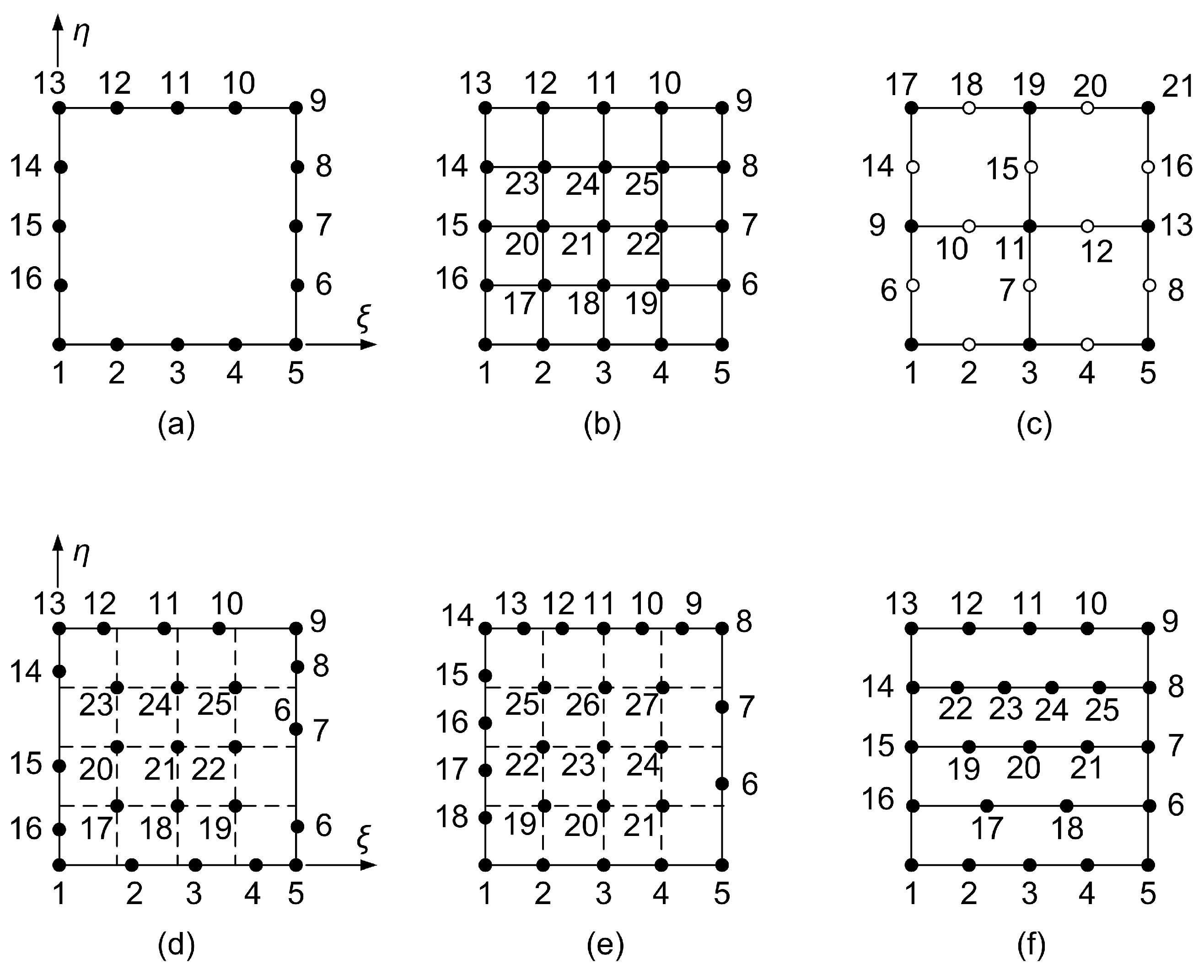
3.6. 27-Node Transfinite Element

As a practical application example, we consider a 27-node transfinite element, of which the four edges are uniformly divided into 4, 3, 6, and 5 segments, respectively, as shown in Figure 5. This means that the associated polynomial degrees per edge are as follows: $p_{AB}=4,p_{BC}=3,p_{DC}=6$, and $P_{AD}=5$. The internal nodes form a uniform tensor product pattern of scheme $3\times 3$ (nodes 19 to 27), which means that the degree of the blending functions is $n_{I,\xi }=n_{I,\eta }=4$ (between edges and internal nodes, four node spans per direction are created). Therefore, this element consists of 18 boundary and 9 internal nodes.

3.6.1. Lagrange–Based Formulation

The implementation of transfinite interpolation (i.e., Equation (1)) to the 27-node element leads to the following set of bivariate shape functions [9]:

$$\begin{array}{cc}\hfill & {\varphi }_1(\xi ,\eta )=L_{1,4}\left(\xi \right)L_{1,5}\left(\eta \right),\hfill \\ \hfill & {\varphi }_2(\xi ,\eta )=L_{2,4}\left(\xi \right)L_{1,4}\left(\eta \right),\hfill \\ \hfill & {\varphi }_3(\xi ,\eta )=L_{3,4}\left(\xi \right)L_{1,4}\left(\eta \right),\hfill \\ \hfill & {\varphi }_4(\xi ,\eta )=L_{4,4}\left(\xi \right)L_{1,4}\left(\eta \right),\hfill \\ \hfill & {\varphi }_5(\xi ,\eta )=L_{5,4}\left(\xi \right)L_{1,3}\left(\eta \right),\hfill \\ \hfill & {\varphi }_6(\xi ,\eta )=L_{5,4}\left(\xi \right)L_{2,3}\left(\eta \right),\hfill \\ \hfill & {\varphi }_7(\xi ,\eta )=L_{5,4}\left(\xi \right)L_{3,3}\left(\eta \right),\hfill \\ \hfill & {\varphi }_8(\xi ,\eta )=L_{4,3}\left(\eta \right)L_{5,4}\left(\xi \right)-L_{5,4}\left(\xi \right)L_{5,4}\left(\eta \right)+L_{5,4}\left(\eta \right)L_{7,6}\left(\xi \right),\hfill \\ \hfill & {\varphi }_9(\xi ,\eta )=L_{5_4}\left(\eta \right)L_{6,6}\left(\xi \right),\hfill \\ \hfill & {\varphi }_{10}(\xi ,\eta )=L_{5_4}\left(\eta \right)L_{5,6}\left(\xi \right),\hfill \\ \hfill & {\varphi }_{11}(\xi ,\eta )=L_{4_6}\left(\xi \right)L_{5,4}\left(\eta \right),\hfill \\ \hfill & {\varphi }_{12}(\xi ,\eta )=L_{3_6}\left(\xi \right)L_{5,4}\left(\eta \right),\hfill \\ \hfill & {\varphi }_{13}(\xi ,\eta )=L_{2,6}\left(\xi \right)L_{5,4}\left(\eta \right),\hfill \\ \hfill & {\varphi }_{14}(\xi ,\eta )=L_{1,6}\left(\xi \right)L_{5,4}\left(\eta \right)-L_{1,4}\left(\xi \right)L_{5,4}\left(\eta \right)+L_{1,4}\left(\xi \right)L_{6,5}\left(\eta \right),\hfill \\ \hfill & {\varphi }_{15}(\xi ,\eta )=L_{1,4}\left(\xi \right)L_{5,5}\left(\eta \right),\hfill \\ \hfill & {\varphi }_{16}(\xi ,\eta )=L_{1,4}\left(\xi \right)L_{4,5}\left(\eta \right),\hfill \\ \hfill & {\varphi }_{17}(\xi ,\eta )=L_{1,4}\left(\xi \right)L_{3,5}\left(\eta \right),\hfill \\ \hfill & {\varphi }_{18}(\xi ,\eta )=L_{1,4}\left(\xi \right)L_{2,5}\left(\eta \right),\hfill \\ \hfill & {\varphi }_{19}(\xi ,\eta )=L_{2,4}\left(\xi \right)L_{2,4}\left(\eta \right),\hfill \\ \hfill & {\varphi }_{20}(\xi ,\eta )=L_{2,4}\left(\eta \right)L_{3,4}\left(\xi \right),\hfill \\ \hfill & {\varphi }_{21}(\xi ,\eta )=L_{2,4}\left(\eta \right)L_{4,4}\left(\xi \right),\hfill \\ \hfill & {\varphi }_{22}(\xi ,\eta )=L_{2,4}\left(\xi \right)L_{3,4}\left(\eta \right),\hfill \\ \hfill & {\varphi }_{23}(\xi ,\eta )=L_{3,4}\left(\xi \right)L_{3,4}\left(\eta \right),\hfill \\ \hfill & {\varphi }_{24}(\xi ,\eta )=L_{3,4}\left(\eta \right)L_{4,4}\left(\xi \right),\hfill \\ \hfill & {\varphi }_{25}(\xi ,\eta )=L_{2,4}\left(\xi \right)L_{4,4}\left(\eta \right),\hfill \\ \hfill & {\varphi }_{26}(\xi ,\eta )=L_{3,4}\left(\xi \right)L_{4,4}\left(\eta \right),\hfill \\ \hfill & {\varphi }_{27}(\xi ,\eta )=L_{4,4}\left(\xi \right)L_{4,4}\left(\eta \right).\hfill \end{array}$$

(60)

Notably, the shape functions ${\varphi }_1(\xi ,\eta )$ and ${\varphi }_5(\xi ,\eta )$, although associated with corner nodes A and B, respectively, consist of only a single term—being influenced solely by the projector $P_{\xi }$. This arises from the second principle of the golden rule, as described in Section 3, whereby the trial functions along the shared edge $AB$ coincide with the corresponding blending functions, which are uniform polynomials of degree 4.

3.6.2. Bernstein–Based Formulation: Model B-1

Setting Bernstein polynomials in the position of blending and trial functions as well, Equation (60) provides the following set of basis functions for model B-1:

$$\begin{array}{cc}\hfill & {\psi }_1(\xi ,\eta )=B_{1,4}\left(\xi \right)B_{1,5}\left(\eta \right),\hfill \\ \hfill & {\psi }_2(\xi ,\eta )=B_{2,4}\left(\xi \right)B_{1,4}\left(\eta \right),\hfill \\ \hfill & {\psi }_3(\xi ,\eta )=B_{3,4}\left(\xi \right)B_{1,4}\left(\eta \right),\hfill \\ \hfill & {\psi }_4(\xi ,\eta )=B_{4,4}\left(\xi \right)B_{1,4}\left(\eta \right),\hfill \\ \hfill & {\psi }_5(\xi ,\eta )=B_{5,4}\left(\xi \right)B_{1,3}\left(\eta \right),\hfill \\ \hfill & {\psi }_6(\xi ,\eta )=B_{5,4}\left(\xi \right)B_{2,3}\left(\eta \right),\hfill \\ \hfill & {\psi }_7(\xi ,\eta )=B_{5,4}\left(\xi \right)B_{3,3}\left(\eta \right),\hfill \\ \hfill & {\psi }_8(\xi ,\eta )=B_{4,3}\left(\eta \right)B_{5,4}\left(\xi \right)-B_{5,4}\left(\xi \right)B_{5,4}\left(\eta \right)+B_{5,4}\left(\eta \right)B_{7,6}\left(\xi \right),\hfill \\ \hfill & {\psi }_9(\xi ,\eta )=B_{5_4}\left(\eta \right)B_{6,6}\left(\xi \right),\hfill \\ \hfill & {\psi }_{10}(\xi ,\eta )=B_{5_4}\left(\eta \right)B_{5,6}\left(\xi \right),\hfill \\ \hfill & {\psi }_{11}(\xi ,\eta )=B_{4_6}\left(\xi \right)B_{5,4}\left(\eta \right),\hfill \\ \hfill & {\psi }_{12}(\xi ,\eta )=B_{3_6}\left(\xi \right)B_{5,4}\left(\eta \right),\hfill \\ \hfill & {\psi }_{13}(\xi ,\eta )=B_{2,6}\left(\xi \right)B_{5,4}\left(\eta \right),\hfill \\ \hfill & {\psi }_{14}(\xi ,\eta )=B_{1,6}\left(\xi \right)B_{5,4}\left(\eta \right)-B_{1,4}\left(\xi \right)B_{5,4}\left(\eta \right)+B_{1,4}\left(\xi \right)B_{6,5}\left(\eta \right),\hfill \\ \hfill & {\psi }_{15}(\xi ,\eta )=B_{1,4}\left(\xi \right)B_{5,5}\left(\eta \right),\hfill \\ \hfill & {\psi }_{16}(\xi ,\eta )=B_{1,4}\left(\xi \right)B_{4,5}\left(\eta \right),\hfill \\ \hfill & {\psi }_{17}(\xi ,\eta )=B_{1,4}\left(\xi \right)B_{3,5}\left(\eta \right),\hfill \\ \hfill & {\psi }_{18}(\xi ,\eta )=B_{1,4}\left(\xi \right)B_{2,5}\left(\eta \right),\hfill \\ \hfill & {\psi }_{19}(\xi ,\eta )=B_{2,4}\left(\xi \right)B_{2,4}\left(\eta \right),\hfill \\ \hfill & {\psi }_{20}(\xi ,\eta )=B_{2,4}\left(\eta \right)B_{3,4}\left(\xi \right),\hfill \\ \hfill & {\psi }_{21}(\xi ,\eta )=B_{2,4}\left(\eta \right)B_{4,4}\left(\xi \right),\hfill \\ \hfill & {\psi }_{22}(\xi ,\eta )=B_{2,4}\left(\xi \right)B_{3,4}\left(\eta \right),\hfill \\ \hfill & {\psi }_{23}(\xi ,\eta )=B_{3,4}\left(\xi \right)B_{3,4}\left(\eta \right),\hfill \\ \hfill & {\psi }_{24}(\xi ,\eta )=B_{3,4}\left(\eta \right)B_{4,4}\left(\xi \right),\hfill \\ \hfill & {\psi }_{25}(\xi ,\eta )=B_{2,4}\left(\xi \right)B_{4,4}\left(\eta \right),\hfill \\ \hfill & {\psi }_{26}(\xi ,\eta )=B_{3,4}\left(\xi \right)B_{4,4}\left(\eta \right),\hfill \\ \hfill & {\psi }_{27}(\xi ,\eta )=B_{4,4}\left(\xi \right)B_{4,4}\left(\eta \right).\hfill \end{array}$$

(61)

3.6.3. Bernstein–Based Formulation: Model B-2

We follow a similar procedure as that of Section 3.4.2. The edge $AB$, which is interpolated with degree $p_{AB}=4$, is written in terms of univariate Bernstein polynomias in $\xi$ and their associate coefficients $a_1,\dots ,a_5$ as follows:

$$U_{AB}\left(\xi \right)=B_{1,4}\left(\xi \right)a_1+B_{2,4}\left(\xi \right)a_2+B_{3,4}\left(\xi \right)a_3+B_{4,4}\left(\xi \right)a_4+B_{5,4}\left(\xi \right)a_5$$

(62)

Similarly, for edge $BC$, which is directed toward $\eta$, we have the following:

$$U_{BC}\left(\eta \right)=B_{1,3}\left(\eta \right)a_5+B_{2,3}\left(\eta \right)a_6+B_{3,3}\left(\eta \right)a_7+B_{4,3}\left(\eta \right)a_8.$$

(63)

For edge $DC$, we have the following:

$$\begin{array}{cc}\hfill U_{DC}\left(\xi \right)& =B_{1,6}\left(\xi \right)a_{14}+B_{2,6}\left(\xi \right)a_{13}+B_{3,6}\left(\xi \right)a_{12}+B_{4,6}\left(\xi \right)a_{11}\hfill \\ \hfill & +B_{5,6}\left(\xi \right)a_{10}+B_{6,6}\left(\xi \right)a_9+B_{7,6}\left(\xi \right)a_8.\hfill \end{array}$$

(64)

Finally, for edge $AD$, which is directed toward $\eta$, we have the following:

$$U_{AD}\left(\eta \right)=B_{1,5}\left(\eta \right)a_1+B_{2,5}\left(\eta \right)a_{18}+B_{3,5}\left(\eta \right)a_{17}+B_{4,5}\left(\eta \right)a_{16}+B_{5,5}\left(\eta \right)a_{15}+B_{6,5}\left(\eta \right)a_{14}.$$

(65)

The above four univariate functions, which are associated with the element edges, are blended as follows:

• The function $U_{AD}\left(\eta \right)$, which is given by Equation (65), is blended by $E_1\left(\xi \right)$.
• The function $U_{BC}\left(\eta \right)$, which is given by Equation (63), is blended by $E_5\left(\xi \right)$.
• The function $U_{AB}\left(\xi \right)$, which is given by Equation (62), is blended by $E_1\left(\eta \right)$.
• The function $U_{DC}\left(\xi \right)$, which is given by Equation (64), is blended by $E_5\left(\eta \right)$.

In more detail, the abovementioned blending functions (of degree 4) are determined using the transformation matrix ${\mathbf{T}}_4$, which is given by Equation (53), and thus the Lagrange-based expression is converted to a Bernstein-based expression, as follows:

$$\begin{array}{cc}\hfill E_1\left(\xi \right)& =B_{1,4}\left(\xi \right)-\frac{13}{12}{B}_{2,4}\left(\xi \right)+\frac{13}{18}{B}_{3,4}\left(\xi \right)-\frac{1}{4}{B}_{4,4}\left(\xi \right),\hfill \end{array}$$

(66)

$$\begin{array}{cc}\hfill E_5\left(\xi \right)& =-\frac{1}{4}{B}_{2,4}\left(\xi \right)+\frac{13}{18}{B}_{3,4}\left(\xi \right)-\frac{13}{12}{B}_{4,4}\left(\xi \right)+B_{5,4}\left(\xi \right),\hfill \end{array}$$

(67)

$$\begin{array}{cc}\hfill E_1\left(\eta \right)& =B_{1,4}\left(\eta \right)-\frac{13}{12}{B}_{2,4}\left(\eta \right)+\frac{13}{18}{B}_{3,4}\left(\eta \right)-\frac{1}{4}{B}_{4,4}\left(\eta \right),\hfill \end{array}$$

(68)

$$\begin{array}{cc}\hfill E_5\left(\eta \right)& =-\frac{1}{4}{B}_{2,4}\left(\eta \right)+\frac{13}{18}{B}_{3,4}\left(\eta \right)-\frac{13}{12}{B}_{4,4}\left(\eta \right)+B_{5,4}\left(\eta \right).\hfill \end{array}$$

(69)

Therefore, the basis functions associated, for example, with the three intermediate nodes of edge $AB$, are given as follows:

$$\begin{array}{cc}\hfill \left[\begin{array}{c}{\overline{\psi }}_2(\xi ,\eta )\\ {\overline{\psi }}_3(\xi ,\eta )\\ {\overline{\psi }}_4(\xi ,\eta )\end{array}\right]& =\left[\begin{array}{c}{B}_{2,4}\left(\xi \right)\\ B_{3,4}\left(\xi \right)\\ B_{4,4}\left(\xi \right)\end{array}\right]E_1\left(\eta \right)\hfill \\ \hfill & =\left[\begin{array}{c}{B}_{2,4}\left(\xi \right)\\ B_{3,4}\left(\xi \right)\\ B_{4,4}\left(\xi \right)\end{array}\right]\left[B_{1,4}\left(\eta \right)-\frac{13}{12}{B}_{2,4}\left(\eta \right)+\frac{13}{18}{B}_{3,4}\left(\eta \right)-\frac{1}{4}{B}_{4,4}\left(\eta \right)\right].\hfill \end{array}$$

(70)

Regarding a corner node, such as node 1 at axis origin, we must consider both projectors toward the $\xi$ and $\eta$ axes and subtract the correcting term, whence the following holds:

$${\overline{\psi }}_1(\xi ,\eta )=B_{1,5}\left(\eta \right)E_1\left(\xi \right)+B_{1,4}\left(\xi \right)E_1\left(\eta \right)-E_1\left(\xi \right)E_1\left(\eta \right).$$

(71)

Moreover, the previous procedure (cf. Equation (57)) is shortened by ignoring the ‘borders’ of the tensor product, and thus the basis functions associated with the internal nodes are found directly by constructing the matrix as follows:

$$\mathbf{I}={\mathbf{T}}_{4,\eta }\left[\begin{array}{c}{B}_{2,4}\left(\eta \right)\\ B_{3,4}\left(\eta \right)\\ B_{4,4}\left(\eta \right)\end{array}\right]\left[\begin{array}{ccc}{B}_{2,4}\left(\xi \right)& B_{3,4}\left(\xi \right)& B_{4,4}\left(\xi \right)\end{array}\right]{\mathbf{T}}_{4,\xi }^T,$$

which is also written as follows:

$$\left[\begin{array}{ccc}4& -32/9& 4/3\\ -3& 20/3& -3\\ 4/3& -32/9& 4\end{array}\right]\left[\begin{array}{c}{B}_{2,4}\left(\eta \right)\\ B_{3,4}\left(\eta \right)\\ B_{4,4}\left(\eta \right)\end{array}\right]\left[\begin{array}{ccc}{B}_{2,4}\left(\xi \right)& B_{3,4}\left(\xi \right)& B_{4,4}\left(\xi \right)\end{array}\right]\left[\begin{array}{ccc}4& -3& 4/3\\ -32/9& 20/3& -32/9\\ 4/3& -3& 4\end{array}\right].$$

(72)

It should be clarified that the associated DOFs with the entries of this matrix are arranged as follows:

$$\left[\begin{array}{ccc}{U}_{19}& U_{20}& U_{21}\\ U_{22}& U_{23}& U_{24}\\ U_{25}& U_{26}& U_{27}\end{array}\right].$$

(73)

Therefore, the result of the multiplications in Equation (72), which is a matrix of size $3\times 3$, of which the nine entries form the basis functions associated with the internal nodes, is as follows:

$$\begin{array}{cc}\hfill {\overline{\psi }}_{19}& =\left(16(9B_{24}\left(\xi \right)-8B_{34}\left(\xi \right)+3B_{44}\left(\xi \right))(9B_{24}\left(\eta \right)-8B_{34}\left(\eta \right)+3B_{44}\left(\eta \right))\right)/81,\hfill \\ \hfill {\overline{\psi }}_{20}& =-\left(4(9B_{24}\left(\eta \right)-8B_{34}\left(\eta \right)+3B_{44}\left(\eta \right))(9B_{24}\left(\xi \right)-20B_{34}\left(\xi \right)+9B_{44}\left(\xi \right))\right)/27,\hfill \\ \hfill {\overline{\psi }}_{21}& =\left(16(3B_{24}\left(\xi \right)-8B_{34}\left(\xi \right)+9B_{44}\left(\xi \right))(9B_{24}\left(\eta \right)-8B_{34}\left(\eta \right)+3B_{44}\left(\eta \right))\right)/81,\hfill \\ \hfill {\overline{\psi }}_{22}& =-\left(4(9B_{24}\left(\xi \right)-8B_{34}\left(\xi \right)+3B_{44}\left(\xi \right))(9B_{24}\left(\eta \right)-20B_{34}\left(\eta \right)+9B_{44}\left(\eta \right))\right)/27,\hfill \\ \hfill {\overline{\psi }}_{23}& =\left((9B_{24}\left(\xi \right)-20B_{34}\left(\xi \right)+9B_{44}\left(\xi \right))(9B_{24}\left(\eta \right)-20B_{34}\left(\eta \right)+9B_{44}\left(\eta \right))\right)/9,\hfill \\ \hfill {\overline{\psi }}_{24}& =-\left(4(3B_{24}\left(\xi \right)-8B_{34}\left(\xi \right)+9B_{44}\left(\xi \right))(9B_{24}\left(\eta \right)-20B_{34}\left(\eta \right)+9B_{44}\left(\eta \right))\right)/27,\hfill \\ \hfill {\overline{\psi }}_{25}& =\left(16(9B_{24}\left(\xi \right)-8B_{34}\left(\xi \right)+3B_{44}\left(\xi \right))(3B_{24}\left(\eta \right)-8B_{34}\left(\eta \right)+9B_{44}\left(\eta \right))\right)/81,\hfill \\ \hfill {\overline{\psi }}_{26}& =-\left(4(3B_{24}\left(\eta \right)-8B_{34}\left(\eta \right)+9B_{44}\left(\eta \right))(9B_{24}\left(\xi \right)-20B_{34}\left(\xi \right)+9B_{44}\left(\xi \right))\right)/27,\hfill \\ \hfill {\overline{\psi }}_{27}& =\left(16(3B_{24}\left(\xi \right)-8B_{34}\left(\xi \right)+9B_{44}\left(\xi \right))(3B_{24}\left(\eta \right)-8B_{34}\left(\eta \right)+9B_{44}\left(\eta \right))\right)/81.\hfill \end{array}$$

(74)

It was found that the element based on Bernstein polynomials, constructed using Equations (70), (71) and (74) (i.e., model B-2), yields the same numerical results as the element based on Lagrange polynomials using Equation (60).

Having found all the basis functions for the 27-node transfinite element, the graphical representation for all the three models is illustrated in Figure 6.

In summary: When the internal nodes of a transfinite element form a tensor product, the number of boundary nodal points can be arbitrary. This means that the same formula can handle a greater or smaller number of boundary nodal points than those determined by the tensor product of the internal nodes.

3.7. Concluding Remark

Regardless of the formulation—whether using Lagrange polynomials or Bernstein polynomials—if the internal nodes are arranged in a tensor product pattern, there is no difficulty in handling any number of boundary nodes. In all cases, the staggered mesh of internal nodes defines the set of blending functions, while the basis functions associated with the internal nodes are simply tensor products of these blending functions. For the basis functions associated with the boundary nodes, they are formed as local tensor products between the univariate trial functions along the current edge and the corresponding blending function in the direction perpendicular to that edge.

Furthermore, to deal with a more difficult class of elements, in which the elements are defined over a structured T-mesh from which several internal nodes have been selectively removed, thus resulting in an incomplete or sparsely populated grid, the reader is referred to Section 5.

3.8. Transitional Transfinite Elemenets

Thus far, we have considered the following classes of transfinite elements:

• Tensor product elements.
• Classical elements with stations holding a standard discretization per direction.
• Distorted tensor product elements.
• Elements with internal nodes in the pattern of a tensor product and arbitrary-noded boundaries.

We now consider elements with internal nodes where the number of nodes per station can vary. A simple case occurs when the nodes (both internal and boundary) are aligned along unidirectional stations—for example, horizontally, as illustrated in Figure 7. For the illustrated 12-node element (Figure 7a), the base functions in terms of Lagrange polynomials are as follows:

$$\begin{array}{cc}\hfill {\varphi }_1(\xi ,\eta )& =L_{1,2}\left(\xi \right)E_1\left(\eta \right),\hfill \\ \hfill {\varphi }_2(\xi ,\eta )& =L_{2,2}\left(\xi \right)E_1\left(\eta \right),\hfill \\ \hfill {\varphi }_3(\xi ,\eta )& =L_{3,2}\left(\xi \right)E_1\left(\eta \right),\hfill \\ \hfill {\varphi }_4(\xi ,\eta )& =L_{1,3}\left(\xi \right)E_2\left(\eta \right),\hfill \\ \hfill {\varphi }_5(\xi ,\eta )& =L_{2,3}\left(\xi \right)E_2\left(\eta \right),\hfill \\ \hfill {\varphi }_6(\xi ,\eta )& =L_{3,3}\left(\xi \right)E_2\left(\eta \right),\hfill \\ \hfill {\varphi }_7(\xi ,\eta )& =L_{3,3}\left(\xi \right)E_2\left(\eta \right),\hfill \\ \hfill {\varphi }_8(\xi ,\eta )& =L_{1,4}\left(\xi \right)E_3\left(\eta \right),\hfill \\ \hfill {\varphi }_9(\xi ,\eta )& =L_{2,4}\left(\xi \right)E_3\left(\eta \right),\hfill \\ \hfill {\varphi }_{10}(\xi ,\eta )& =L_{3,4}\left(\xi \right)E_3\left(\eta \right),\hfill \\ \hfill {\varphi }_{11}(\xi ,\eta )& =L_{4,4}\left(\xi \right)E_3\left(\eta \right),\hfill \\ \hfill {\varphi }_{12}(\xi ,\eta )& =L_{5,4}\left(\xi \right)E_3\left(\eta \right).\hfill \end{array}$$

(75)

The graph of global shape functions is illustrated in Figure 8a.

Next, replacing Lagrange with their counterpart Bernstein polynomials (model B-1), we receive the following set of non-negative basis functions:

$$\begin{array}{cc}\hfill {\psi }_1(\xi ,\eta )& =B_{1,2}\left(\xi \right)B_{1,2}\left(\eta \right),\hfill \\ \hfill {\psi }_2(\xi ,\eta )& =B_{2,2}\left(\xi \right)B_{1,2}\left(\eta \right),\hfill \\ \hfill {\psi }_3(\xi ,\eta )& =B_{3,2}\left(\xi \right)B_{1,2}\left(\eta \right),\hfill \\ \hfill {\psi }_4(\xi ,\eta )& =B_{1,3}\left(\xi \right)B_{2,2}\left(\eta \right),\hfill \\ \hfill {\psi }_5(\xi ,\eta )& =B_{2,3}\left(\xi \right)B_{2,2}\left(\eta \right),\hfill \\ \hfill {\psi }_6(\xi ,\eta )& =B_{3,3}\left(\xi \right)B_{2,2}\left(\eta \right),\hfill \\ \hfill {\psi }_7(\xi ,\eta )& =B_{3,3}\left(\xi \right)B_{2,2}\left(\eta \right),\hfill \\ \hfill {\psi }_8(\xi ,\eta )& =B_{1,4}\left(\xi \right)B_{3,2}\left(\eta \right),\hfill \\ \hfill {\psi }_9(\xi ,\eta )& =B_{2,4}\left(\xi \right)B_{3,2}\left(\eta \right),\hfill \\ \hfill {\psi }_{10}(\xi ,\eta )& =B_{3,4}\left(\xi \right)B_{3,2}\left(\eta \right),\hfill \\ \hfill {\psi }_{11}(\xi ,\eta )& =B_{4,4}\left(\xi \right)B_{3,2}\left(\eta \right),\hfill \\ \hfill {\psi }_{12}(\xi ,\eta )& =B_{5,4}\left(\xi \right)B_{3,2}\left(\eta \right).\hfill \end{array}$$

(76)

The graph of basis functions is illustrated in Figure 8b.

As we will demonstrate in the Results Section 6, the sets of shape and basis functions defined by Equations (75) and (76), respectively, are not fully equivalent and therefore lead to slightly different results. Consequently, there does not exist a transformation matrix $\mathbf{R}$ satisfying the relation $\mathsf{\varphi }=\mathbf{R}\mathsf{\psi }$. However, since the quality of the approximation in model B-1 remains satisfactory, there is no necessity to pursue an exact representation of the Lagrange polynomials in terms of Bernstein polynomials.

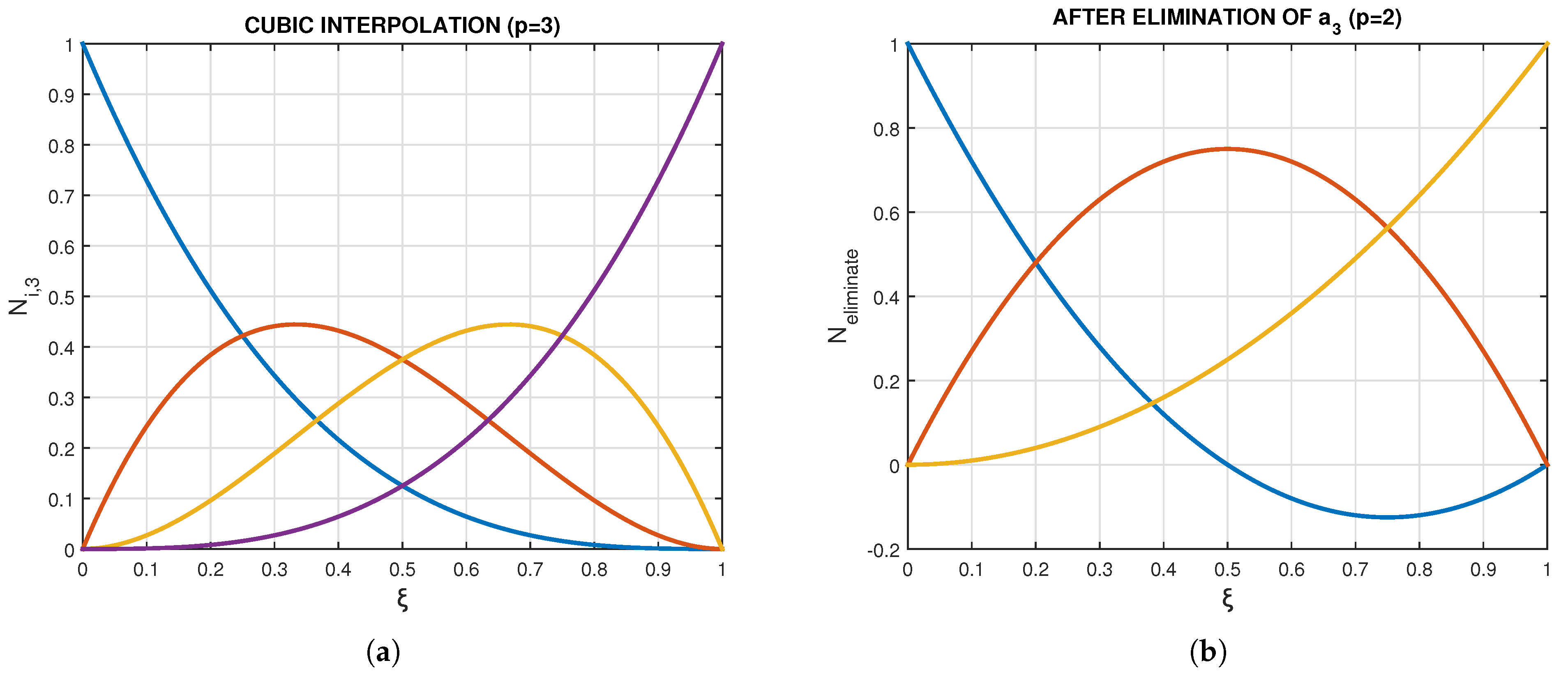
4. Reduction of Bernstein Polynomials

A very recent study has shown that the treatment of the interior in T-meshed elements can be facilitated by the observation that a Lagrange polynomial can be generated by a higher-order Lagrange polynomial, provided that certain linear constraints are imposed [10]. For example, a linear polynomial defined between the endpoints $\xi =0$ and $\xi =1$ can be reproduced by a quadratic polynomial based on nodes at ${\xi }_1=0$, ${\xi }_2={\displaystyle \frac{1}{2}}$, and ${\xi }_3=1$, provided the constraint $U_2={\displaystyle \frac{U_1+U_3}{2}}$ is enforced (see Figure 9a). Similarly, a uniform quadratic polynomial based on nodal points at $\xi =0$, ${\displaystyle \frac{1}{3}}$, and 1 can be generated by a cubic polynomial by imposing the constraint $U_3=-{\displaystyle \frac{U_1}{3}}+U_2+{\displaystyle \frac{U_4}{3}}$ (see Figure 9b), and so forth. In summary, when Lagrange polynomials of degrees $p=1,2,3$ are used, for the characteristic configurations shown in Figure 9, the corresponding constraints are as follows (see Ref. [10]):

$$\begin{array}{cc}\hfill \mathrm{Linear}(\mathrm{Figure}9\mathrm{a})& :U_2={\displaystyle \frac{U_1+U_3}{2}},\hfill \end{array}$$

(77)

$$\begin{array}{cc}\hfill \mathrm{Quadratic}(\mathrm{Figure}9\mathrm{b})& :U_3=-{\displaystyle \frac{U_1}{3}}+U_2+{\displaystyle \frac{U_4}{3}},\hfill \end{array}$$

(78)

$$\begin{array}{cc}\hfill \mathrm{Cubic}-1(\mathrm{Figure}9\mathrm{c})& :U_2={\displaystyle \frac{U_1}{4}}+{\displaystyle \frac{3}{2}}{U}_3-U_4+{\displaystyle \frac{U_5}{4}},\hfill \end{array}$$

(79)

$$\begin{array}{cc}\hfill \mathrm{Cubic}-2(\mathrm{Figure}9\mathrm{d})& :U_3=-{\displaystyle \frac{U_1}{6}}+{\displaystyle \frac{2}{3}}{U}_2+{\displaystyle \frac{2}{3}}{U}_4-{\displaystyle \frac{U_5}{6}}.\hfill \end{array}$$

(80)

For example, regarding cubic interpolation with a missing node in midpoint (Figure 9d), if the corresponding constraint imposed for $U_3$ by Equation (80) is inserted into a sum of Lagrange polynomials of degree 4 ($U={\sum }_{i=1}^5{L}_{i,4}{U}_i$), the expression degenerates to a sum of Lagrange polynomials of degree 3 ($U={\sum }_{j=1}^4{L}_{j,3}{U}_i$), which are illustrated in Figure 10a. The solid line corresponds to Lagrange polynomials of degree 3 which were directly calculated, whereas the markers by small circles correspond to the degenerated Lagrange polynomials of degree 4 after imposing Equation (80). Note that if the same procedure is applied to the Bernstein polynomials for the coefficient $a_3$, the resulting modified cubic Bernstein polynomials—derived from those of degree 4—do not coincide with the true cubic polynomials (see Figure 10b). Nevertheless, the condition imposed by Equation (80) is again fulfilled, as shown in Appendix B.

Remark 2. 

It is noted that, not only one, but more nodal points can be eliminated, either consecutively or simultaneously. Obviously, the number of the eliminated nodes is the number of the constraints imposed.

Within the context of the paper at hand, it was found that the above constraints remain invariable when Bernstein polynomials are used, merely by substituting the nodal values $U_i$ by the coefficents $a_i$. For example, if we impose the constraint $a_2={\displaystyle \frac{a_1+a_3}{2}}$ to a set of three quadratic Bernstein polynomials ($B_0={(1-\xi )}^2,B_1=2(1-\xi )\xi ,B_2={\xi }^2$), one may easily verify that they eventually reduce to a set of two linear Bernstein polynomials (${\tilde{B}}_0=1-\xi ,{\tilde{B}}_1=\xi$).

For the purposes of the paper at hand, we reduce ourselves to recast the above constraints in terms of generalized coefficients as follows:

$$\begin{array}{cc}\hfill \mathrm{Linear}& :a_2={\displaystyle \frac{a_1+a_3}{2}},\hfill \end{array}$$

(81)

$$\begin{array}{cc}\hfill \mathrm{Quadratic}& :a_3=-{\displaystyle \frac{a_1}{3}}+a_2+{\displaystyle \frac{a_4}{3}},\hfill \end{array}$$

(82)

$$\begin{array}{cc}\hfill \mathrm{Cubic}-1& :a_2={\displaystyle \frac{a_1}{4}}+{\displaystyle \frac{3}{2}}{a}_3-a_4+{\displaystyle \frac{a_5}{4}},\hfill \end{array}$$

(83)

$$\begin{array}{cc}\hfill \mathrm{Cubic}-2& :a_3=-{\displaystyle \frac{a_1}{6}}+{\displaystyle \frac{2}{3}}{a}_2+{\displaystyle \frac{2}{3}}{a}_4-{\displaystyle \frac{a_5}{6}}.\hfill \end{array}$$

(84)

Related to this, as a special case (alternative to the direct procedure presented in Appendix B), it will be shown below that a cubic polynomial similarly degenerates into a quadratic one.

Cubic polynomials and quadratic constraints: To make the study meaningful, the intermediate (internal) node is taken at one-third measured from the left end. Clearly, we have a unit length with three nodes as follows: 1 (at $\xi =0$), 2 (at $\xi =1/3$), and 4 (at $\xi =1$), as illustrated in Figure 9b, thus creating non-uniform Lagrange of degree two. In the previously mentioned sequence, node ‘3’ was omitted because it is eliminated from the uniform sequence of four nodes, 1-2-3-4, and thus only the nodes 1-2-4 remain. In more detail, we start from the uniform sequence where the transformation matrix between Lagrange and Bernstein polynomials is as follows (see, ([7], p.267)):

$$\left[\begin{array}{c}{L}_{1,3}\left(\xi \right)\\ L_{2,3}\left(\xi \right)\\ L_{3,3}\left(\xi \right)\\ L_{4,3}\left(\xi \right)\end{array}\right]=\left[\begin{array}{cccc}1& -{\displaystyle \frac{5}{6}}& {\displaystyle \frac{1}{3}}& 0\\ 0& 3& -{\displaystyle \frac{3}{2}}& 0\\ 0& -{\displaystyle \frac{3}{2}}& 3& 0\\ 0& {\displaystyle \frac{1}{3}}& -{\displaystyle \frac{5}{6}}& 1\end{array}\right]\left[\begin{array}{c}{B}_{1,3}\left(\xi \right)\\ B_{2,3}\left(\xi \right)\\ B_{3,3}\left(\xi \right)\\ B_{4,3}\left(\xi \right)\end{array}\right],$$

(85)

whereas the relationship between nodal values and coefficients depends on the transpose of the transformation matrix involved in Equation (85), and thus is as follows:

$$\left[\begin{array}{c}{a}_1\\ a_2\\ a_3\\ a_4\end{array}\right]=\left[\begin{array}{cccc}1& 0& 0& 0\\ -{\displaystyle \frac{5}{6}}& 3& -{\displaystyle \frac{3}{2}}& {\displaystyle \frac{1}{3}}\\ {\displaystyle \frac{1}{3}}& -{\displaystyle \frac{3}{2}}& 3& -{\displaystyle \frac{5}{6}}\\ 0& 0& 0& 1\end{array}\right]\left[\begin{array}{c}{U}_1\\ U_2\\ U_3\\ U_4\end{array}\right].$$

(86)

Inverting Equation (86), we receive the following:

$$\left[\begin{array}{c}{U}_1\\ U_2\\ U_3\\ U_4\end{array}\right]=\left[\begin{array}{cccc}1& 0& 0& 0\\ {\displaystyle \frac{8}{27}}& {\displaystyle \frac{4}{9}}& {\displaystyle \frac{2}{9}}& {\displaystyle \frac{1}{27}}\\ {\displaystyle \frac{1}{27}}& {\displaystyle \frac{2}{9}}& {\displaystyle \frac{4}{9}}& {\displaystyle \frac{8}{27}}\\ 0& 0& 0& 1\end{array}\right]\left[\begin{array}{c}{a}_1\\ a_2\\ a_3\\ a_4\end{array}\right].$$

(87)

Clearly, the above equalities refer to the uniform case in which the nodal points are located at $\xi =0,{\displaystyle \frac{1}{3}},{\displaystyle \frac{2}{3}},1$. Now, we start with the simple case of Lagrange polynomials, where node ‘3’ is missing. This in turn means that if we consider the value $U_3$ produced by the non-uniform polynomial of degree 2 at node 3 as a constraint in terms of $(U_1,U_2,U_4)$, if the latter is introduced into the series expansion of four (cubic) Lagrange polynomials, we shall identically derive the expression of the non-uniform quadratic polynomial.

As has been previously found in Ref. [10], it is trivial to show that the three non-uniform polynomials (based on the nodal values, ${\xi }_1=0,{\xi }_2=1/3,{\xi }_4=1$) lead to the following constraint (at ${\xi }_3=2/3$):

$$U_3=-{\displaystyle \frac{1}{3}}{U}_1+U_2+{\displaystyle \frac{1}{3}}{U}_4.$$

(88)

Substituting in Equation (88) the four nodal values $U_i,i=1,\dots 4$ in terms of $a_i,i=1,\dots 4$, by Equation (87), we eventually obtain the following:

$$a_3=-{\displaystyle \frac{1}{3}}{a}_1+a_2+{\displaystyle \frac{1}{3}}{a}_4.$$

(89)

Comparing Equation (88) with Equation (89), we see that for a univariate interpolation (such as that along an edge), the constraint imposed for node 3 is identical in form—either nodal value U or arbitrary coefficients a are used. Since the tensor product, which may be the starting point for performing elimination (imposition of constraints) is identical for either Lagrange or Bernstein polynomials, the same constraint in them (cf. Equation (88) and Equation (89)) ensures the same final expression, in which the Lagrange polynomials are blindly substituted by Bernstein polynomials of the same degree. In this sense, the 18-node transfinite element has the same expression in either set of polynomials, and an obviously linear relationship will occur between the column vectors, including the 18 shape functions (local tensor products).

A rigorous proof for the degeneration of a quartic polynomial to a cubic one is given in Appendix B, whereas the general mathematical proof for any degree n is given in Appendix C.

The general theoretical explanation for this event is as follows:

The similarity between constrained expressions in Lagrange and Bernstein bases arises from the affine invariance of polynomial spaces. Since both bases span the same space, any affine transformation of the parameter domain preserves polynomial expressions. The Bernstein basis, defined via barycentric coordinates, and the Lagrange basis, constructed from the interpolation conditions, are related through a linear transformation. As a result, any linear constraint on function values remains unchanged when expressed in either basis.

Non-Uniform Lagrange Polynomials

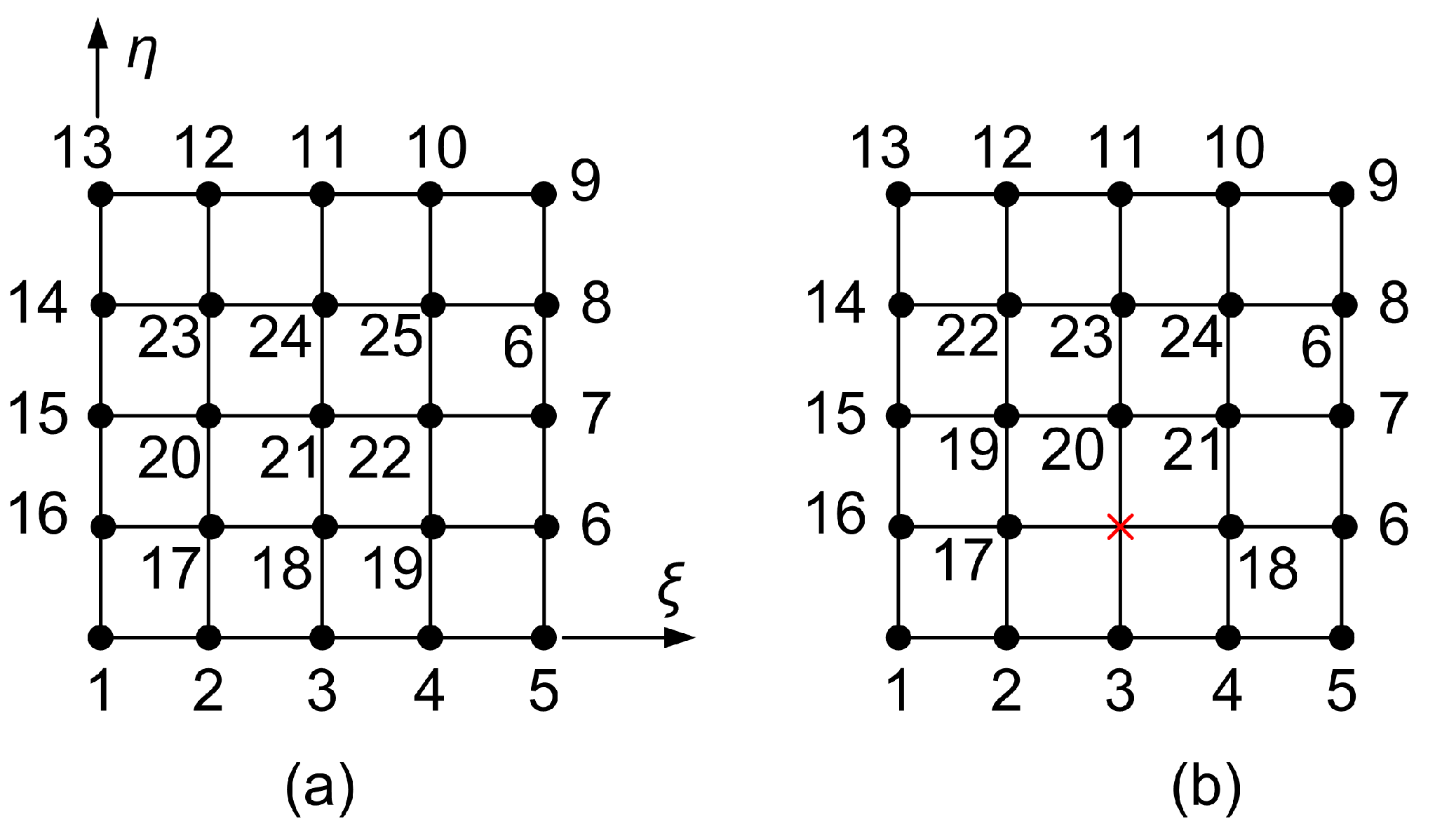
The standard expressions for the transformation matrices $\mathbf{T}$, which have been reported in previous papers [7,8] have been derived for uniform (equally spaced) Lagrange polynomials. However, when the intermediate nodes on a line segment (in the parametrc interval $[0,1]$) are moved from their initial uniform position, the set of nodal points on which Lagrange polynomials are based changes, merely because the nodal values $U_i$ change. In contrast, Bernstein polynomials are of standard form according to Equation (23), and thus, they do not depend on the position of the associated control points. In conclusion, the change of nodal points along a segment implies a change of the transformation matrix $\mathbf{T}$ and a change of the generalized coefficients. The collocation at nodal points gives ${\mathbf{U}}_{\mathrm{nodal}}=\mathbf{C}\mathbf{a}$. For each position of internal nodes with value ${\mathbf{U}}_{\mathrm{nodal}}$, the matrix $\mathbf{C}$ takes a different value, and the vector of the coefficient becomes $\mathbf{a}={\mathbf{C}}^{-1}{\mathbf{U}}_{\mathrm{nodal}}$, whence $\mathbf{T}={\left({\mathbf{C}}^t\right)}^{-1}$.

5. T-Mesh Elements

In general, two broad methodologies exist for constructing finite elements with T-junctions, applicable to both Lagrange and Bernstein polynomial bases. The first approach is based on transfinite interpolation, implemented through one or more directional projections. The second approach employs sequential processing on a tensor product background, where internal nodes are progressively eliminated. The case involving Lagrange polynomials has been examined in detail in Ref. [10].

For the sake of completeness, this paper revisits the Lagrange polynomial formulation but primarily focuses on a systematic investigation of the performance of Bernstein polynomials. As previously noted, both the Lagrange and Bernstein formulations distinguish between boundary and interior nodes of a T-mesh element. However, this distinction becomes more pronounced in the context of a T-mesh.

5.1. Simplified T-Elements

With reference to the tensor product element shown in Figure 11a, two representative T-elements are illustrated in Figure 11b,c. These are obtained by initially removing two boundary nodes (3 and 5), followed by the removal of one internal node (14). In all three configurations, the internal nodes are arranged to form two internal stations per direction, located at $\xi ={\displaystyle \frac{1}{3}},{\displaystyle \frac{2}{3}}$ and $\eta ={\displaystyle \frac{1}{3}},{\displaystyle \frac{2}{3}}$. This simplified example serves as a basis for the subsequent discussion on the derivation of basis functions.

5.2. Boundary Nodes

5.2.1. The 13-, 14- and 15-Node Elements

In Figure 11b–d, one may observe that the nodal sequence along $AB$ is $\xi =[0,{\displaystyle \frac{1}{3}},1]$, as also is the case with Figure 9b. The missing node at the position $G(\xi ={\displaystyle \frac{2}{3}})$, which is denoted by a skew cross (×), is described by Equation (89) (i.e., $a_3=-{\displaystyle \frac{1}{3}}{a}_1+a_2+{\displaystyle \frac{1}{3}}{a}_4$).

Substituting Equation (89) into the usual univariate interpolation along the edge $AB$ (with $\eta =0$) using cubic Bernstein polynomials as follows:

$$U(\xi ,0)=B_{1,3}\left(\xi \right)a_1+B_{2,3}\left(\xi \right)a_2+B_{3,3}\left(\xi \right)a_3+B_{4,3}\left(\xi \right)a_4,$$

(90)

we eventually eliminate $a_3$ (associated with point G), and thus receive:

$$U(\xi ,0)=\underset{{\overline{B}}_1\left(\xi \right)}{\underbrace{\left(B_{1,3}\left(\xi \right)-{\displaystyle \frac{1}{3}}{B}_{3,3}\left(\xi \right)\right)}}{a}_1+\underset{{\overline{B}}_2\left(\xi \right)}{\underbrace{\left(B_{2,3}\left(\xi \right)+B_{3,3}\left(\xi \right)\right)}}{a}_2+\underset{{\overline{B}}_3\left(\xi \right)}{\underbrace{\left(B_{4,3}\left(\xi \right)+{\displaystyle \frac{1}{3}}{B}_{3,3}\left(\xi \right)\right)}}{a}_4.$$

(91)

The univariate basis functions ($B_{1,3},B_{2,3},B_{3,3},B_{4,3}$) along the edge $AB$, associated with initial nodal points (1,2,3,4; shown in Figure 11a), and (${\overline{B}}_1,{\overline{B}}_2,{\overline{B}}_3$), associated with the final nodes (1,2,3; shown in Figure 11b–d), are illustrated in Figure 12a and Figure 12b, respectively. One may observe that while the conventional Bernstein polynomials are non-negative (see Figure 12a), those produced after the elimination may take negative values as well (see Figure 12b). In more detail, one may verify that the updated polynomials in Equation (91) are as follows: ${\overline{B}}_1\left(\xi \right)=2{\xi }^2-3\xi +1,{\overline{B}}_2\left(\xi \right)=-3{\xi }^2+3\xi$, and ${\overline{B}}_3\left(\xi \right)={\xi }^2$. They also hold the partition of unity property, i.e., ${\overline{B}}_1\left(\xi \right)+{\overline{B}}_2\left(\xi \right)+{\overline{B}}_3\left(\xi \right)\equiv 1$ for $0\le \xi \le 1$.

Based on the three modified univariate trial functions ${\overline{B}}_i$ involved in Equation (91) and shown in Figure 12b, in the T-mesh element $ABCD$, the bivariate basis functions which correspond to the edge $AB$ can be easily determined.

Next, we apply either the transfinite interpolation formula (first approach) or the background tensor product technique (second approach). In both cases using bivariate Bernstein polynomials of degree 3 ($B_{i,3}$ for $i=1,2,3,4$), the basis functions for the 15-node element (see Figure 11b), organized by horizontal layers, are defined as follows:

$$\begin{array}{cc}\hfill {\psi }_1(\xi ,\eta )& =\left(B_{1,3}\left(\xi \right)-\frac{1}{3}{B}_{3,3}\left(\xi \right)\right)B_{1,3}\left(\eta \right),\hfill \\ \hfill {\psi }_2(\xi ,\eta )& =\left(B_{2,3}\left(\xi \right)+B_{3,3}\left(\xi \right)\right)B_{1,3}\left(\eta \right),\hfill \\ \hfill {\psi }_3(\xi ,\eta )& =\left(B_{4,3}\left(\xi \right)+\frac{1}{3}{B}_{3,3}\left(\xi \right)\right)B_{1,3}\left(\eta \right),\hfill \\ \hfill {\psi }_{11}(\xi ,\eta )& =B_{1,3}\left(\xi \right)B_{2,3}\left(\eta \right),\hfill \\ \hfill {\psi }_{12}(\xi ,\eta )& =B_{2,3}\left(\xi \right)B_{2,3}\left(\eta \right),\hfill \\ \hfill {\psi }_{13}(\xi ,\eta )& =B_{3,3}\left(\xi \right)B_{2,3}\left(\eta \right),\hfill \\ \hfill {\psi }_4(\xi ,\eta )& =B_{4,3}\left(\xi \right)B_{2,3}\left(\eta \right),\hfill \\ \hfill {\psi }_{10}(\xi ,\eta )& =B_{1,3}\left(\xi \right)B_{3,3}\left(\eta \right),\hfill \\ \hfill {\psi }_{14}(\xi ,\eta )& =B_{2,3}\left(\xi \right)B_{3,3}\left(\eta \right),\hfill \\ \hfill {\psi }_{15}(\xi ,\eta )& =B_{3,3}\left(\xi \right)B_{3,3}\left(\eta \right),\hfill \\ \hfill {\psi }_5(\xi ,\eta )& =B_{4,3}\left(\xi \right)B_{3,3}\left(\eta \right),\hfill \\ \hfill {\psi }_9(\xi ,\eta )& =B_{1,3}\left(\xi \right)B_{4,3}\left(\eta \right),\hfill \\ \hfill {\psi }_8(\xi ,\eta )& =B_{2,3}\left(\xi \right)B_{4,3}\left(\eta \right),\hfill \\ \hfill {\psi }_7(\xi ,\eta )& =B_{3,3}\left(\xi \right)B_{4,3}\left(\eta \right),\hfill \\ \hfill {\psi }_6(\xi ,\eta )& =B_{4,3}\left(\xi \right)B_{4,3}\left(\eta \right).\hfill \end{array}$$

(92)

One may observe that only the first three DOFs, which are associated with the bottom edge $AB$, are affected by the consideration of the constraint.

Since the underlying approach is based on the tensor product structure, it is immaterial whether it is applied using Bernstein or Lagrange polynomials. Consequently, if the goal is to obtain the shape functions ${\varphi }_i$, for $i=1,\dots ,15$, associated with Lagrange polynomials, it suffices to replace the Bernstein polynomials $B_{i,3}$ (for $i=1,2,3,4$) in Equation (92) with their corresponding Lagrange polynomials $L_{i,3}$. Consequently, the set of basis functions ${\psi }_i$ included in Equation (92) is equivalent (but not identical in form) to the following set:

$$\begin{array}{cc}\hfill {\varphi }_1(\xi ,\eta )& =\left(L_{1,3}\left(\xi \right)-\frac{1}{3}{L}_{3,3}\left(\xi \right)\right)L_{1,3}\left(\eta \right),\hfill \\ \hfill {\varphi }_2(\xi ,\eta )& =\left(L_{2,3}\left(\xi \right)+L_{3,3}\left(\xi \right)\right)L_{1,3}\left(\eta \right),\hfill \\ \hfill {\varphi }_3(\xi ,\eta )& =\left(L_{4,3}\left(\xi \right)+\frac{1}{3}{L}_{3,3}\left(\xi \right)\right)L_{1,3}\left(\eta \right),\hfill \\ \hfill {\varphi }_{11}(\xi ,\eta )& =L_{1,3}\left(\xi \right)L_{2,3}\left(\eta \right),\hfill \\ \hfill {\varphi }_{12}(\xi ,\eta )& =L_{2,3}\left(\xi \right)L_{2,3}\left(\eta \right),\hfill \\ \hfill {\varphi }_{13}(\xi ,\eta )& =L_{3,3}\left(\xi \right)L_{2,3}\left(\eta \right),\hfill \\ \hfill {\varphi }_4(\xi ,\eta )& =L_{4,3}\left(\xi \right)L_{2,3}\left(\eta \right),\hfill \\ \hfill {\varphi }_{10}(\xi ,\eta )& =L_{1,3}\left(\xi \right)L_{3,3}\left(\eta \right),\hfill \\ \hfill {\varphi }_{14}(\xi ,\eta )& =L_{2,3}\left(\xi \right)L_{3,3}\left(\eta \right),\hfill \\ \hfill {\varphi }_{15}(\xi ,\eta )& =L_{3,3}\left(\xi \right)L_{3,3}\left(\eta \right),\hfill \\ \hfill {\varphi }_5(\xi ,\eta )& =L_{4,3}\left(\xi \right)L_{3,3}\left(\eta \right),\hfill \\ \hfill {\varphi }_9(\xi ,\eta )& =L_{1,3}\left(\xi \right)L_{4,3}\left(\eta \right),\hfill \\ \hfill {\varphi }_8(\xi ,\eta )& =L_{2,3}\left(\xi \right)L_{4,3}\left(\eta \right),\hfill \\ \hfill {\varphi }_7(\xi ,\eta )& =L_{3,3}\left(\xi \right)L_{4,3}\left(\eta \right),\hfill \\ \hfill {\varphi }_6(\xi ,\eta )& =L_{4,3}\left(\xi \right)L_{4,3}\left(\eta \right).\hfill \end{array}$$

(93)

The abovementioned equivalence was also verified by a numerical example reported in Section 6, in which both models give the same numerical result. Here, in advance, we report that the common value was $L_2=0.2600\%$ for the solution of the boundary value problem, and $L_2=0.2679\%$ for the interpolation problem based on exact nodal values.

5.2.2. 14-Node Element

The 14-node element shown in Figure 11c needs further processing. In addition to the constraint $a_3=-{\displaystyle \frac{1}{3}}{a}_1+a_2+{\displaystyle \frac{1}{3}}{a}_4$ which refers to the bottom edge $AB$ (point G), we also consider a second constraint regarding the edge $BC$ (point F), i.e.,

$$a_5={\displaystyle \frac{1}{3}}{a}_4+a_6-{\displaystyle \frac{1}{3}}{a}_7,$$

(94)

where ($a_4,a_6,a_7$) refer to the initial background mesh illustrated in Figure 11a. Substituting Equations (89) and (94) into the initial tensor product, for node numbering as illustrated in Figure 11c, we eventually receive the following:

$$\begin{array}{cc}\hfill {\varphi }_1(\xi ,\eta )& =\left(L_{1,3}\left(\xi \right)-\frac{1}{3}{L}_{3,3}\left(\xi \right)\right)L_{1,3}\left(\eta \right),\hfill \\ \hfill {\varphi }_2(\xi ,\eta )& =\left(L_{2,3}\left(\xi \right)+L_{3,3}\left(\xi \right)\right)L_{1,3}\left(\eta \right),\hfill \\ \hfill {\varphi }_3(\xi ,\eta )& =\left(\frac{1}{3}{L}_{3,3}\left(\xi \right)+L_{4,3}\left(\xi \right)\right)L_{1,3}\left(\eta \right)+\frac{1}{3}{L}_{4,3}\left(\xi \right)L_{2,3}\left(\eta \right),\hfill \\ \hfill {\varphi }_4(\xi ,\eta )& =L_{4,3}\left(\xi \right)\left(L_{2,3}\left(\eta \right)+L_{3,3}\left(\eta \right)\right),\hfill \\ \hfill {\varphi }_5(\xi ,\eta )& =L_{4,3}\left(\xi \right)\left(L_{4,3}\left(\eta \right)-\frac{1}{3}{L}_{2,3}\left(\eta \right)\right),\hfill \\ \hfill {\varphi }_6(\xi ,\eta )& =L_{3,3}\left(\xi \right)L_{4,3}\left(\eta \right),\hfill \\ \hfill {\varphi }_7(\xi ,\eta )& =L_{2,3}\left(\xi \right)L_{4,3}\left(\eta \right),\hfill \\ \hfill {\varphi }_8(\xi ,\eta )& =L_{1,3}\left(\xi \right)L_{4,3}\left(\eta \right),\hfill \\ \hfill {\varphi }_9(\xi ,\eta )& =L_{1,3}\left(\xi \right)L_{3,3}\left(\eta \right),\hfill \\ \hfill {\varphi }_{10}(\xi ,\eta )& =L_{1,3}\left(\xi \right)L_{2,3}\left(\eta \right),\hfill \\ \hfill {\varphi }_{11}(\xi ,\eta )& =L_{2,3}\left(\xi \right)L_{2,3}\left(\eta \right),\hfill \\ \hfill {\varphi }_{12}(\xi ,\eta )& =L_{3,3}\left(\xi \right)L_{2,3}\left(\eta \right),\hfill \\ \hfill {\varphi }_{13}(\xi ,\eta )& =L_{2,3}\left(\xi \right)L_{3,3}\left(\eta \right),\hfill \\ \hfill {\varphi }_{14}(\xi ,\eta )& =L_{3,3}\left(\xi \right)L_{3,3}\left(\eta \right).\hfill \end{array}$$

(95)

It can be observed that only the first five degrees of freedom (DOFs), which are associated with the edges $AB$ and $BC$ where the two constraints are imposed, are affected—thereby altering the tensor product structure. In particular, the corner node ‘3’ is influenced by two blending functions as follows: $L_{1,3}\left(\eta \right)$ in the $\eta$-direction and $L_{4,3}\left(\xi \right)$ in the $\xi$-direction.

The associated model B-1 is the same as in Equation (95) where Lagrange polynomials $L_{i,3}$ are merely substituted by Bernstein polynomials $B_{i,3},i=1,2,3,4$.

Again, the same error was found ($L_2=0.2600\%$) for Lagrange and Bernstein polynomials.

5.2.3. 13-Node Element

The 13-node configuration—shown in Figure 11d—still requires further processing. Relative to the tensor product mesh in Figure 11a, node ‘14’ (point E in Figure 11d) could be constrained once along the horizontal line 12–13–14–5 and again along the vertical line 3–14–16–8.

Therefore, from the constraint in the $\xi$-direction,

$$a_{14}=-{\displaystyle \frac{1}{3}}{a}_{12}+a_{13}+{\displaystyle \frac{1}{3}}{a}_5,,$$

(96)

and from the constraint in the $\eta$-direction,

$$a_{14}={\displaystyle \frac{1}{3}}{a}_3+a_{16}-{\displaystyle \frac{1}{3}}{a}_8.$$

(97)

Then, although it is possible to work considering one of these two options, it is more reasonable to take the mean average as follows:

$$a_{14}={\displaystyle \frac{1}{2}}\left(-{\displaystyle \frac{1}{3}}{a}_{12}+a_{13}+{\displaystyle \frac{1}{3}}{a}_5\right)+{\displaystyle \frac{1}{2}}\left({\displaystyle \frac{1}{3}}{a}_3+a_{16}-{\displaystyle \frac{1}{3}}{a}_8\right).$$

(98)

Therefore, for the 13-node element under consideration, the totality of the constraints—applicable to the tensor product—is as follows: Equations (89), (94) and (98). Considering all of them, the initial tensor product of Lagrange polynomials degenerates to the following final shape functions:

$$\begin{array}{cc}\hfill {\varphi }_1& =L_{1,3}\left(\xi \right)L_{1,3}\left(\eta \right)-\left(L_{3,3}\left(\xi \right)L_{1,3}\left(\eta \right)\right)/3-\left(L_{3,3}\left(\xi \right)L_{2,3}\left(\eta \right)\right)/18,\hfill \\ \hfill {\varphi }_2& =L_{2,3}\left(\xi \right)L_{1,3}\left(\eta \right)+L_{3,3}\left(\xi \right)L_{1,3}\left(\eta \right)+\left(L_{3,3}\left(\xi \right)L_{2,3}\left(\eta \right)\right)/6,\hfill \\ \hfill {\varphi }_3& =\left(L_{3,3}\left(\xi \right)L_{1,3}\left(\eta \right)\right)/3+\left(L_{3,3}\left(\xi \right)L_{2,3}\left(\eta \right)\right)/9+L_{4,3}\left(\xi \right)L_{1,3}\left(\eta \right)+\left(L_{4,3}\left(\xi \right)L_{2,3}\left(\eta \right)\right)/3,\hfill \\ \hfill {\varphi }_4& =\left(L_{3,3}\left(\xi \right)L_{2,3}\left(\eta \right)\right)/6+L_{4,3}\left(\xi \right)L_{2,3}\left(\eta \right)+L_{4,3}\left(\xi \right)L_{3,3}\left(\eta \right),\hfill \\ \hfill {\varphi }_5& =L_{4,3}\left(\xi \right)L_{4,3}\left(\eta \right)-\left(L_{4,3}\left(\xi \right)L_{2,3}\left(\eta \right)\right)/3-\left(L_{3,3}\left(\xi \right)L_{2,3}\left(\eta \right)\right)/18,\hfill \\ \hfill {\varphi }_6& =L_{3,3}\left(\xi \right)L_{4,3}\left(\eta \right)-\left(L_{3,3}\left(\xi \right)L_{2,3}\left(\eta \right)\right)/6,\hfill \\ \hfill {\varphi }_7& =L_{2,3}\left(\xi \right)L_{4,3}\left(\eta \right),\hfill \\ \hfill {\varphi }_8& =L_{1,3}\left(\xi \right)L_{4,3}\left(\eta \right),\hfill \\ \hfill {\varphi }_9& =L_{1,3}\left(\xi \right)L_{3,3}\left(\eta \right),\hfill \\ \hfill {\varphi }_{10}& =L_{1,3}\left(\xi \right)L_{2,3}\left(\eta \right)-\left(L_{3,3}\left(\xi \right)L_{2,3}\left(\eta \right)\right)/6,\hfill \\ \hfill {\varphi }_{11}& =L_{2,3}\left(\xi \right)L_{2,3}\left(\eta \right)+\left(L_{3,3}\left(\xi \right)L_{2,3}\left(\eta \right)\right)/2,\hfill \\ \hfill {\varphi }_{12}& =L_{2,3}\left(\xi \right)L_{3,3}\left(\eta \right),\hfill \\ \hfill {\varphi }_{13}& =\left(L_{3,3}\left(\xi \right)L_{2,3}\left(\eta \right)\right)/2+L_{3,3}\left(\xi \right)L_{3,3}\left(\eta \right).\hfill \end{array}$$

(99)

Similarly, the initial tensor product of Bernsten polynomials degenerates to the following final basis functions:

$$\begin{array}{cc}\hfill {\psi }_1& =B_{1,3}\left(\xi \right)B_{1,3}\left(\eta \right)-\left(B_{3,3}\left(\xi \right)B_{1,3}\left(\eta \right)\right)/3-\left(B_{3,3}\left(\xi \right)B_{2,3}\left(\eta \right)\right)/18,\hfill \\ \hfill {\psi }_2& =B_{2,3}\left(\xi \right)B_{1,3}\left(\eta \right)+B_{3,3}\left(\xi \right)B_{1,3}\left(\eta \right)+\left(B_{3,3}\left(\xi \right)B_{2,3}\left(\eta \right)\right)/6,\hfill \\ \hfill {\psi }_3& =\left(B_{3,3}\left(\xi \right)B_{1,3}\left(\eta \right)\right)/3+\left(B_{3,3}\left(\xi \right)B_{2,3}\left(\eta \right)\right)/9+B_{4,3}\left(\xi \right)B_{1,3}\left(\eta \right)+\left(B_{4,3}\left(\xi \right)B_{2,3}\left(\eta \right)\right)/3,\hfill \\ \hfill {\psi }_4& =\left(B_{3,3}\left(\xi \right)B_{2,3}\left(\eta \right)\right)/6+B_{4,3}\left(\xi \right)B_{2,3}\left(\eta \right)+B_{4,3}\left(\xi \right)B_{3,3}\left(\eta \right),\hfill \\ \hfill {\psi }_5& =B_{4,3}\left(\xi \right)B_{4,3}\left(\eta \right)-\left(B_{4,3}\left(\xi \right)B_{2,3}\left(\eta \right)\right)/3-\left(B_{3,3}\left(\xi \right)B_{2,3}\left(\eta \right)\right)/18,\hfill \\ \hfill {\psi }_6& =B_{3,3}\left(\xi \right)B_{4,3}\left(\eta \right)-\left(B_{3,3}\left(\xi \right)B_{2,3}\left(\eta \right)\right)/6,\hfill \\ \hfill {\psi }_7& =B_{2,3}\left(\xi \right)B_{4,3}\left(\eta \right),\hfill \\ \hfill {\psi }_8& =B_{1,3}\left(\xi \right)B_{4,3}\left(\eta \right),\hfill \\ \hfill {\psi }_9& =B_{1,3}\left(\xi \right)B_{3,3}\left(\eta \right),\hfill \\ \hfill {\psi }_{10}& =B_{1,3}\left(\xi \right)B_{2,3}\left(\eta \right)-\left(B_{3,3}\left(\xi \right)B_{2,3}\left(\eta \right)\right)/6,\hfill \\ \hfill {\psi }_{11}& =B_{2,3}\left(\xi \right)B_{2,3}\left(\eta \right)+\left(B_{3,3}\left(\xi \right)B_{2,3}\left(\eta \right)\right)/2,\hfill \\ \hfill {\psi }_{12}& =B_{2,3}\left(\xi \right)B_{3,3}\left(\eta \right),\hfill \\ \hfill {\psi }_{13}& =\left(B_{3,3}\left(\xi \right)B_{2,3}\left(\eta \right)\right)/2+B_{3,3}\left(\xi \right)B_{3,3}\left(\eta \right).\hfill \end{array}$$

(100)

In contrast to the previous element of Section 5.2.2, in the 13-node element, the errors of two formulations differ as follows: $L_{2L}=0.4030\%$ (Lagrange) and $L_{2B}=0.2775\%$ (Bernstein).

5.3. Internal Nodes

A distinguishing feature of the elements considered in this section is that the density of internal nodes dictates the maximum polynomial degree in each parametric direction ($n_{\xi },n_{\eta }$). Clearly, unlike the elements discussed in Section 3.5, we assume that there are no edges with a polynomial degree exceeding that imposed by the internal node distribution. This is not a disadvantage, as the same holds in older [11] and current accepted models of T-spline [12,13,14,15,16].

Regarding the internal nodes, if the grid is complete, it suffices to consider the full tensor product of either Lagrange or Bernstein polynomials. In more details,

• If the objective is to construct a Lagrange-based polynomial model, one begins with a tensor product of Lagrange polynomials, which is subsequently modified—through constraints—to account for any missing internal nodes. This issue has been previously discussed in full detail in Ref. [10].
• If the objective is to construct a Bernstein-based model, one begins with a tensor product of Bernstein polynomials, which is subsequently modified to account for any missing internal nodes. This is the main topic of this paper.

This raises the question: Do the internal nodes influence the bivariate basis functions associated with the boundary?

First of all, we have to say that the univariate interpolation on each of the four edges is entirely independent on the other edges as well as on the interior. In case that the internal nodes are arranged in a compact tensor product (like in Figure 13a), the aforementioned interpolation functions of the boundary are merely blended using those blending functions determined by the internal nodes, as depicted by Equation (44).

Nevertheless, when at least one internal node is missing from the compact tensor product pattern, it has some influence on some boundary nodes as well. This happens despite the fact that the boundary itself is not influenced, but only the action of the associated bivariate basis functions inside the domain. More specifically, the influence depends on the selection which isoline/station will be considered or not considered. To aid understanding, we first considered a tensor product element (Figure 13a), which was then modified into a 24-node element by removing the central node from the bottom layer of internal nodes (Figure 13b). In both configurations, node numbering begins along the same boundary and proceeds inward to the interior nodes.

5.3.1. Lagrange Polynomials

In this context, working with Lagrange polynomials, we have the following:

• The elimination of the middle node along the horizontal station 16-17-18-6 (Figure 13b) is made either considering a non-uniform polynomial of degree 3 for which the transfinite interpoltion is $U(\xi ,\eta )=P_{\eta }$, or by the following constraint:

  $$U_{\mathrm{delete},\mathrm{x}}=-1/16U_{16}+2/3U_{17}+2/3U_{18}-1/6U_6,$$

  (101)
• The elimination of the middle node along the vertical station (made of nodes 3-20-23-11) is made either considering a non-uniform polynomial of degree 3 for which the transfinite approximation is $U(\xi ,\eta )=P_{\xi }$ or using the following constraint:

  $$U_{\mathrm{delete},\mathrm{y}}=1/4U_3+3/2U_{20}-U_{23}+1/4U_{11},$$

  (102)
• Alternatively, we may consider the average of the above two considerations for the eliminated DOF as follows:

  $$\begin{array}{cc}\hfill U_{\mathrm{delete}}& ={\displaystyle \frac{1}{2}}(U_{\mathrm{delete},\mathrm{x}}+U_{\mathrm{delete},\mathrm{y}})\hfill \\ \hfill & =(-{\displaystyle \frac{1}{32}}{U}_{16}+{\displaystyle \frac{1}{3}}{U}_{17}+{\displaystyle \frac{1}{3}}{U}_{18}-{\displaystyle \frac{1}{12}}{U}_6)+\hfill \\ \hfill & ({\displaystyle \frac{1}{8}}{U}_3+{\displaystyle \frac{3}{4}}{U}_{20}-{\displaystyle \frac{1}{2}}{U}_{23}+{\displaystyle \frac{1}{8}}{U}_{11}),\hfill \end{array}$$

  (103)

5.3.2. Bernstein Polynomials

In the sequence, we study the Bernstein-based model, starting from the tensor product of them. Our findings are as follows:

• When the bottom (horizontal) layer is considered as a non-uniform polynomial of degree 3, the approximation is $U(\xi ,\eta )=P_{\eta }$. Alternatively, the associated constraint is as follows:

  $$a_{\mathrm{delete},\mathrm{x}}=-1/16a_{16}+2/3a_{17}+2/3a_{18}-1/6a_6.$$

  (104)
• When the middle (vertical) layer is considered as a non-uniform polynomial of degree 3, the approximation is $U(\xi ,\eta )=P_{\xi }$. Alternatively, the associated constraint is as follows:

  $$a_{\mathrm{delete},\mathrm{y}}=1/4a_3+3/2a_{20}-a_{23}+1/4a_{11},$$

  (105)
• When the average of the above two approximations is considered, the associated constraint is as follows:

  $$a_{\mathrm{delete}}={\displaystyle \frac{1}{2}}(-1/16a_{16}+2/3a_{17}+2/3a_{18}-1/6a_6)+{\displaystyle \frac{1}{2}}(1/4a_3+3/2a_{20}-a_{23}+1/4a_{11}).$$

  (106)

As will be verified in section ‘Results’ (Section 6.2), one may observe that all three Bernstein-based models are very similar, but again the average model is closer to the first model which performs the elimination toward $\xi$-direction.

In all cases, the average model is on the safe side.

A useful observation is that, the removal of node 25 from the middle bottom layer of internal nodes, influences those boundary nodes which constitute the ends of the stations to which the eliminated node is considered to belong. For example, when we consider that node 25 belongs to the horizontal station 16-17-18-6, the basis functions associated with nodes 16 and 6 are influenced. Moreover, when we consider that node 25 belongs to the vertical station 3-20-23-11, the basis functions associated with nodes 3 and 11 are influenced. Finally, when node 25 is considered to both of them (at their intersection, taking the average), all the four boundary nodes (16, 6, 3, 11) are influenced.

6. Results

In all cases, the reported error norm $L_2$ is defined (in percent %) as follows:

$$L_2={\left[{\displaystyle \frac{{\int \int }_{\mathsf{\Omega }}{(u_{\mathrm{calculated}}-u_{\mathrm{exact}})}^{2}d\mathsf{\Omega }}{{\int \int }_{\mathsf{\Omega }}{\left(u_{\mathrm{exact}}\right)}^{2}d\mathsf{\Omega }}}\right]}^{1/2}\times 100(\%),$$

(107)

where $u_{\mathrm{calculated}}$ and $u_{\mathrm{exact}}$ are the calculated and exact values of the variable $U(\xi ,\eta )$, respectively, over the entire domain $\mathsf{\Omega }$.

In this paper, several models will be studied. In brief, they concern the following:

• 9-node element (Figure 3a and Figure 14b).
• 11-node element (Figure 3b and Figure 14c).
• 12-node element (Figure 7a).
• 18-node element (Figure 7b).
• 24-node element (Figure 13b).
• 25-node element (Figure 13a).
• 27-node element (Figure 5).
• 46-node element (Figure 15).

In all cases, Lagrange and Bernstein polynomials will be used. In the second case of Bernstein polynomials, two models (model B-1 and model B-2) will be reported. Example 1 concerns the quality of interpolation based on given values at the nodal points of the single square element which models the entire patch. Example 2 refers to the numerical solution of a BVP with a non-polynomial exact solution. Example 3 is concerned with the Poisson equation in a standard benchmark problem.

6.1. Small-Size Models with Fully Populated Interior

The simplest case of a transfinite element is the 9-node element which is illustrated in Figure 3a. In this case, it can be readily shown that the tensor product of Lagrange polynomials is mathematically equivalent to the corresponding tensor product of Bernstein polynomials. Difficulties arise when deviating from the tensor product pattern—for example, when two additional nodes (e.g., nodes 10 and 11) are introduced along the top edge of the domain (Figure 3b). Nevertheless, this issue was successfully treated in Section 3.

Example 1. 

Approximation of mathematical function in square domain.

The only reason for this example is that it has been used in [8], where it was the only reported case that Lagrange and Bernstein polynomials do not lead to the same numerical result. To check whether this previous finding is valid, we present here results for the same function but in smaller models, in which a rapid convergence occurs.

Let us consider the function $U(x,y)=e^{x}cos\left(\pi y\right)$, which is collocated at all 9 or 11 nodal points, accordingly, of the square element. Based on these 9 or 11 nodal values ($U_1,\dots ,U_{11}$), the overall error norm was found to be as shown in

Table 1. Error norm $L_2$ (in %) for the approximation of function $U(x,y)=e^{x}cos\left(\pi y\right)$ within a square domain (9, 11, 12, and 18 DOFs).

Element Type	Lagrange Polynomials	Bernstein: Model B-1	Bernstein: Model B-2
	Equation (22)	Equation (29)	Equation (40)
9-node	21.2377	21.2377	21.2377
11-node	21.2870	21.2879	21.2870
12-node	21.2870	21.2870	–
18-node	0.9024	0.9033	–

. As theory dictates, for the tensor product element, all formulations are equivalent and lead to the same numerical result. For the non-tensor 11-node element, Table 1 shows that the numerical finding is marginally in favor of the Lagrange-based formulation (compared to model B-1). The slight increase in the $L_2$ error norm when transitioning from the 9-node to the 11-node element is incidental, as will be confirmed by the other numerical results presented below.

In the sequence, the same elements were used to obtain the numerical solution of a BVP (Example 2), governed by a Laplace equation. The characteristic of this problem is that the problem is fully two-dimensional and also the exact solution is of non-polynomial form.

Example 2. 

Heat-flow in rectangular sheet.

Let us consider a square sheet of dimensions $(a=b=1)$ in which the Laplace equation dominates $({\nabla }^{2}U=0)$. The boundary conditions are partially of Dirichlet and Neumann type, as shown in Figure 14a. The temperature along the top edge is given as

$$U(x,y=b)=U_{m}cos\left({\displaystyle \frac{\pi x}{2a}}\right),0\le x\le a.$$

(108)

The exact solution is given as follows:

$$U(x,y)=U_m{\displaystyle \frac{sinh\left(\frac{\pi y}{2a}\right)}{sinh\left(\frac{\pi b}{2a}\right)}}cos\left({\displaystyle \frac{\pi x}{2a}}\right),0\le x\le a,0\le y\le b.$$

(109)

Solution: The entire patch $ABCD$ was discretized as a single transfinite element of either 9 or 11 degrees of freedom (DOFs), shown in Figure 14b,c (with polynomial degrees $p_x=2$ and $p_y=2$), of which only two DOFs (i.e., nodes 4 and 5) are unrestrained. The results are a follows:

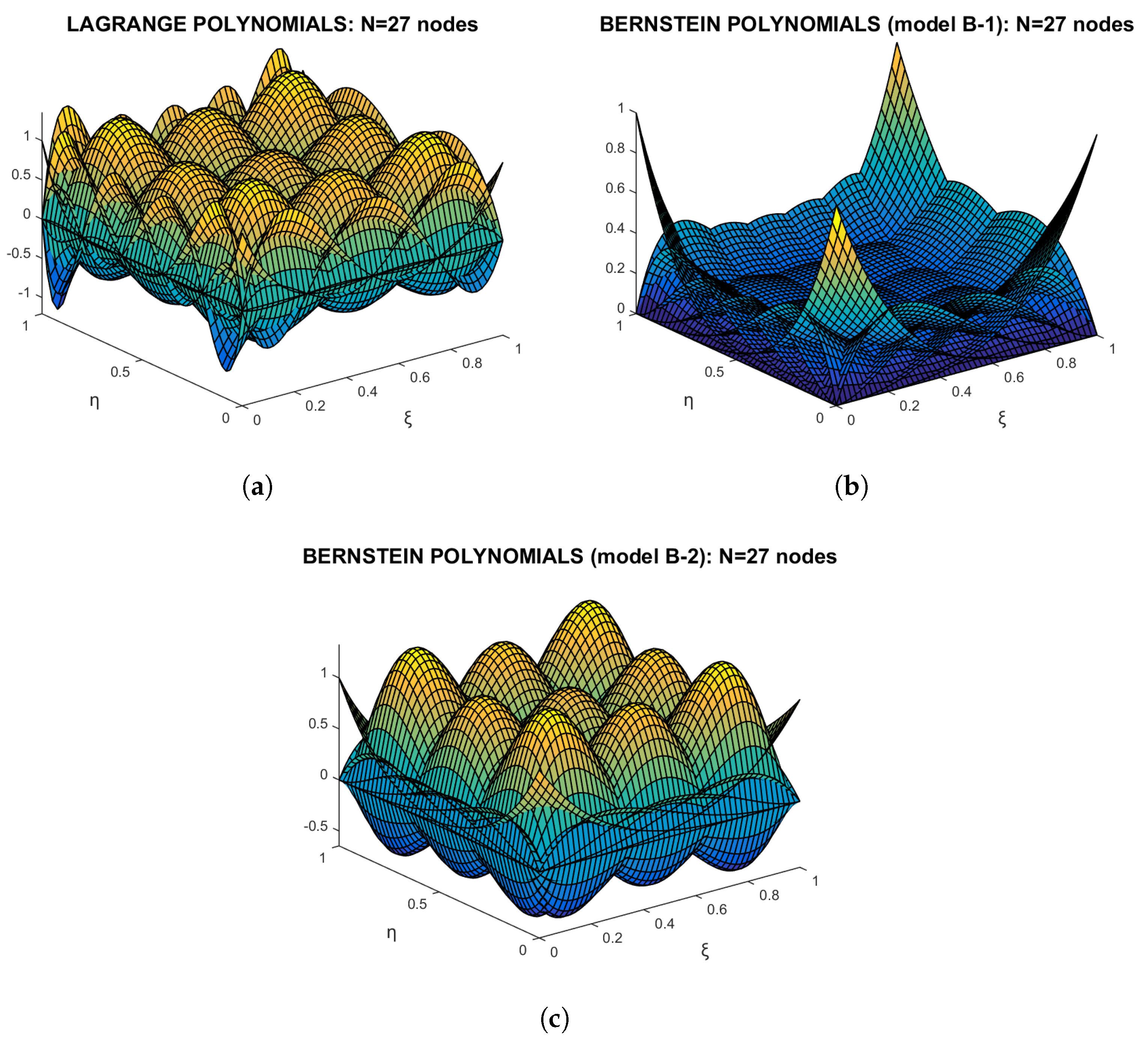
• Regarding the tensor product 9-node element (Figure 14b), using either Lagrange or Bernstein polynomials, the calculated error was found to be the same, equal to $L_2=3.2235\%$ (see

  Table 2. Error norm $L_2$ (in %) from the solution of a BVP into a square sheet (9, 11, 12, and 18 DOFs).

  Element Type	Lagrange Polynomials	Bernstein: Model B-1	Bernstein: Model B-2
  	Equation (22)	Equation (29)	Equation (40)
  9-node	3.2235	3.2235	3.2235
  11-node	2.8567	2.6875	2.8567
  12-node	2.6671	2.6655	–
  18-node	0.1638	0.1556	–

  ). The only difference in the two numerical solutions was the condition number of the equations’ matrix (of size $2\times 2$), which was found equal to 41.8 and 55.3 for Lagrange and Bernstein polynomials, respectively.
• Regarding the non-tensor product 11-node element (Figure 14c), the numerical results for the plate with cosine-like temperature, are shown in the last line of Table 2. One may observe that the Bernstein-based model B-2 (Equation (40)) is equivalent to the Lagrange-based model, where the Bernstein-based model B-1 (Equation (29)) is marginally better.
• Regarding the non-tensor product 12-node element (Figure 7a), the difference between Lagrange and Bernstein polynomials (model B-1) is minor, and thus, we attempted to develop model B-2.
• In all cases, as the model increases the accuracy improves.

In addition, using the same elements, after collocation of the exact nodal values at the 9 or 11 points, we derived the results shown in

Table 3. Error norm $L_2$ (in %) for the approximation of function $U(x,y)=U_{m}sinh\left(\pi y2a\right)/sinh\left(\pi b/2a\right)cos\left(\pi x/2a\right)$ within a square domain (9, 11, 12, and 18 DOFs).

Element Type	Lagrange Polynomials	Bernstein: Model B-1	Bernstein: Model B-2
	Equation (22)	Equation (29)	Equation (40)
9-node	3.1905	3.1905	3.1905
11-node	2.9028	2.6920	2.9028
12-node	2.6721	2.6691	–
18-node	0.1641	0.1543	–

(Lagrange, 2.9028%; Bernstein, 2.6920%). The latter results are very close to those obtained in the BVP.

6.2. Medium-Size Models

This refers to a uniform arrangement of $5\times 5$ nodes, as shown in Figure 13. Starting with the full tensor product grid of 25 nodes as a reference, we select one internal node and remove it from the mesh. The removal of an internal node is treated as its elimination along the station (row or column) it belongs to. We are particularly interested in studying whether, and how, the elimination of an internal node affects the behavior of the nearby boundary.

In this context, working with Lagrange polynomials, we have the following:

• When the bottom (horizontal) layer (made of nodes 16-17-18-6) is considered as a non-uniform polynomial of degree 3, the transfinite approximation becomes $U(\xi ,\eta )=P_{\eta }$, and the error of the numerical solution is $L_2=0.0409\%$. The same result is obtained when inserting the constraint given by Equation (101) into the tensor product of Lagrange polynomials.
• When the middle (vertical) layer (made of nodes 3-20-23-11) is considered as a non-uniform polynomial of degree 3, the transfinite approximation is $U(\xi ,\eta )=P_{\xi }$, and the numerical result is $L_2=0.0892\%$. The same result is obtained when inserting the constraint given by Equation (102) into the tensor product of Lagrange polynomials.
• When the average of the above two considerations was taken for the eliminated DOF according to Equation (103), the result was $L_2=0.0498\%$.
• Regarding tensor product solution (25 nodes), Lagrange polynomials led to the same numerical error equal to $L_2,(\mathrm{tensor}-\mathrm{product})=0.0232\%$.

One may observe that the average-based model is closer to the reasonable first choice, i.e., of considering $U(\xi ,\eta )=P_{\eta }$.

Moreover, working with Bernstein polynomials, we have the following:

• When the bottom (horizontal) layer is considered as a non-uniform polynomial of degree 3, the approximation is $U(\xi ,\eta )=P_{\eta }$, and the result is $L_2=0.0240\%$. The same result is obtained when inserting the constraint ($a_{\mathrm{delete}}=-1/16a_{16}+2/3a_{17}+2/3a_{18}-1/6a_6$) of Equation (104) into the tensor product.
• When the middle (vertical) layer is considered as a non-uniform polynomial of degree 3, the approximation is $U(\xi ,\eta )=P_{\xi }$ and the result is $L_2=0.0263\%$. The same result is obtained when inserting the constraint ($a_{\mathrm{delete}}=1/4a_3+3/2a_{20}-a_{23}+1/4a_{11}$) of Equation (105) into the tensor product.
• When the average of the above two considerations was taken for the eliminated DOF, i.e., ($a_{\mathrm{delete}}={\displaystyle \frac{1}{2}}(-1/16a_{16}+2/3a_{17}+2/3a_{18}-1/6a_6)+{\displaystyle \frac{1}{2}}(1/4a_3+3/2a_{20}-a_{23}+1/4a_{11})$) of Equation (106), the result was $L_2=0.0242\%$.
• Regarding tensor product solution (25 nodes), Bernstein polynomials led to the same numerical error equal to $L_2,(\mathrm{tensor}-\mathrm{product})=0.0232\%$.

One may observe that all three Bernstein-based models are very similar, but again, the average model is closer to the first model, which performs the elimination toward the $\xi$-direction.

In all cases, the average model is on the safe side.

A useful observation is that, the removal of node 25 from the middle bottom layer of internal nodes influences those boundary nodes which constitute the ends of the stations to which the eliminated node is considered to belong. For example, when we consider that 25 belongs to the horizontal station 16-17-18-6, the basis functions associated with nodes 16 and 6 are influenced. Moreover, when we consider that 25 belongs to the vertical station 3-20-23-11, the basis functions associated with nodes 3 and 11 are influenced. Finally, when node 25 is considered to both of them (at their intersection, taking the average), all four boundary nodes (16,6,3, and 11) are influenced.

Regarding tensor product solution (25 nodes), both Lagrange and Bernstein polynomials led to the same numerical error equal to $L_2,(\mathrm{tensor}-\mathrm{product})=0.0232\%$.

6.3. Large-Size Model

The 46-node T-mesh, illustrated in Figure 15a, has been taken from Ref. [10], where the construction of this element has been fully explained.

In brief, it consists of 46 nodes whereas the corresponding background tensor product includes 81 nodes. This means that 35 constraints have been imposed in the auxiliary DOFs. Among them, 32 constraints refer to single stations as follows: 15 DOFs on horizontal stations, red-colored cross (×); and 17 DOFs on vertical stations, cyan-colored cross (×). The rest three DOFs, denoted by green-colored crosses (×), correspond to station intersections.

Lagrange polynomial formulation: The closed-form of the 46 shape functions based on the Lagrange polynomials’ model are very lengthy and may be found in the Appendix of Ref. [10]. As an illustrative example in this paper, the shape function ${\varphi }_1(\xi ,\eta )$, corresponding to corner node ‘1’, is presented in Equation (A17) of Appendix E.1.

Bernstein polynomial formulation (Model B-1): In the context of this paper, for model B-1, we applied the same constraints to the coefficients $a_i$ instead of the nodal values $U_i$. The final result is that the produced Bernstein polynomials’ model consists of the same expressions of basis functions as those in the abovementioned Lagrange polynomials’ model. In other words, the various Lagrange polynomials of degree 8 were merely substituted by their counterpart Bernstein polynomials of the same degree. Indicatively, the basis function ${\psi }_1(\xi ,\eta )$ associated with the corner node ‘1’ is given in Equation (A18) of Appendix E.2.

Regarding the accuracy of the 46-node element in Example 2, Ref. [10] reports an $L_2$ error norm of 0.0115% using the Lagrange polynomial model. When (in the shape functions) Lagrange polynomials were replaced with Bernstein polynomials (Model B-1), the error was slightly reduced to 0.0072% (see

Table 4. Error norm $L_2$ (in %) and condition numbers for the numerical solution of two BVPs within a 46-node square T-element.

Problem Type	Lagrange Polynomials	Bernstein: Model B-1	Bernstein: Model B-2
	Equation (22)	Equation (29)	Equation (40)
Example 2	0.0115	0.0072	0.0115
Condition Number	$6.79\times {10}^3$	$2.37\times {10}^4$	$2.16\times {10}^7$
Example 3	0.0225	0.0042	0.0225
Condition Number	$3.83\times {10}^3$	$2.36\times {10}^4$	$2.15\times {10}^7$

, Example 2, third column).

Bernstein polynomial formulation (Model B-2): Next, we consider Model B-2, in which Lagrange polynomials are replaced by their equivalent Bernstein polynomials. This substitution requires the construction of the one-dimensional transformation matrix ${\mathbf{T}}_8$, which is analogous to those defined in Equations (51)–(55). The matrix ${\mathbf{T}}_8$ can be computed numerically by first forming a $9\times 9$ matrix ${\overline{\mathbf{T}}}_8$ whose entries are univariate Bernstein polynomials, i.e., ${\overline{t}}_{ij}=B_{i,8}\left({\xi }_j\right)$, evaluated at nine uniform places, i.e., ${\xi }_1=0,{\xi }_2=1/8,\dots ,{\xi }_8=7/8,{\xi }_9=1$. The desired matrix is then given by ${\mathbf{T}}_8={\left({\overline{\mathbf{T}}}_8^T\right)}^{-1}$. Consequently, the column vector ${\mathbf{L}}_8$, comprising the nine Lagrange polynomials of degree 8 in either $\xi$ or $\eta$, can be directly expressed in terms of the corresponding column vector ${\mathbf{B}}_8$ of Bernstein polynomials via the relation ${\mathbf{L}}_8={\mathbf{T}}_8{\mathbf{B}}_8$. This expression can then be substituted into Equation (A17) of Appendix E.1, and the subsequent derivations proceed accordingly. In the end, this procedure yields the same shape functions ${\varphi }_i(\xi ,\eta )$, now expressed in terms of Bernstein polynomials rather than Lagrange polynomials. The implementation of this procedure is straightforward and is left as an exercise for the reader.

An alternative formulation to Model B-2 is presented as follows. We begin with the tensor product representation of Bernstein polynomials,

$$U(\xi ,\eta )=\sum _{i=1}^9\sum _{j=1}^9{B}_{i,8}\left(\xi \right)B_{j,8}\left(\eta \right)a_{ij},$$

(110)

which is mathematically equivalent to the tensor product of Lagrange polynomials. By applying Equation (110) to a uniform $9\times 9$ grid of points, we numerically derive a transformation matrix $\mathbf{T}$ of size $81\times 81$ so that the nodal value vector ${\mathbf{U}}_{\mathrm{nodal}}$ is given in terms of generalized coefficients $\mathbf{a}$ by

$${\mathbf{U}}_{\mathrm{nodal}}=\mathbf{T}\mathbf{a}.$$

(111)

The vector ${\mathbf{U}}_{\mathrm{nodal}}$ of size $81\times 1$ splits in two sets, the former being the primary nodal values ${\mathbf{U}}_p$ (i.e., $U_1$ to $U_{46}$) and the latter the secondary values ${\mathbf{U}}_s$ (i.e., $U_{47}$ to $U_{81}$). Similarly, the vector $\mathbf{A}$ including the generalized coefficients (of size $81\times 1$) splits in two sets, the former being the primary ${\mathbf{A}}_p$ (i.e., $a_1$ to $a_{46}$) and the latter the secondary values ${\mathbf{A}}_s$ (i.e., $a_{47}$ to $a_{81}$).

We then consider the 35 constraint equations formulated in terms of the variable U, where the secondary DOFs are expressed in terms of the primary DOFs, through a matrix $S_u$ of size $35\times 46$, by the following:

$${\mathbf{U}}_{\mathrm{s}}={\mathbf{S}}_u{\mathbf{U}}_p.$$

(112)

It is worthy to mention that if between secondary (${\mathbf{A}}_s$) and primary (${\mathbf{A}}_p$) generalized coefficients we consider the same transformation matrix ${\mathbf{S}}_u$, then we get the abovementioned Model B-1. In contrast, below we get a very equivalent form of the U-based constraints, and this is implemented as follows.

Equation (111) splits into the following two parts:

$$\left[\begin{array}{c}{\mathbf{U}}_p\\ {\mathbf{U}}_s\end{array}\right]=\mathbf{T}\left[\begin{array}{c}{\mathbf{A}}_p\\ {\mathbf{A}}_s\end{array}\right]$$

(113)

By inverting Equation (113), we obtain the following useful relationship:

$$\left[\begin{array}{c}{\mathbf{A}}_p\\ {\mathbf{A}}_s\end{array}\right]={\left(\mathbf{T}\right)}^{-1}\left[\begin{array}{c}{\mathbf{U}}_p\\ {\mathbf{U}}_s\end{array}\right]=\left[\begin{array}{cc}{\left({\mathbf{T}}_{pp}\right)}_{\mathrm{inv}}& {\left({\mathbf{T}}_{ps}\right)}_{\mathrm{inv}}\\ {\left({\mathbf{T}}_{sp}\right)}_{\mathrm{inv}}& {\left({\mathbf{T}}_{ss}\right)}_{\mathrm{inv}}\end{array}\right]\left[\begin{array}{c}{\mathbf{U}}_p\\ {\mathbf{U}}_s\end{array}\right],$$

(114)

which splits into the following two equations:

$$\begin{array}{cc}\hfill {\mathbf{A}}_p& ={\left({\mathbf{T}}_{pp}\right)}_{\mathrm{inv}}{\mathbf{U}}_p+{\left({\mathbf{T}}_{ps}\right)}_{\mathrm{inv}}{\mathbf{U}}_s,\hfill \end{array}$$

(115)

$$\begin{array}{cc}\hfill {\mathbf{A}}_s& ={\left({\mathbf{T}}_{sp}\right)}_{\mathrm{inv}}{\mathbf{U}}_p+{\left({\mathbf{T}}_{ss}\right)}_{\mathrm{inv}}{\mathbf{U}}_s.\hfill \end{array}$$

(116)

Solving Equation (115) in ${\mathbf{U}}_p$ and then substituting into Equation (116) (i.e., eliminating ${\mathbf{U}}_p$), the linear relationship between the primary and secondary coefficients is found as

$${\mathbf{A}}_{\mathrm{s}}={\mathbf{S}}_a{\mathbf{A}}_p.$$

(117)

where the transformation matrix is given by

$${\mathbf{S}}_a=\left[{\left({\mathbf{T}}_{sp}\right)}_{\mathrm{inv}}+{\left({\mathbf{T}}_{ss}\right)}_{\mathrm{inv}}{\mathbf{S}}_u\right]{\left[{\left({\mathbf{T}}_{pp}\right)}_{\mathrm{inv}}+{\left({\mathbf{T}}_{ps}\right)}_{\mathrm{inv}}{\mathbf{S}}_u\right]}^{-1}.$$

(118)

Substituting the secondary coefficients ${\mathbf{A}}_s$ (using the combination of Equations (117) and (118)) into the tensor product of Equation (110), we eventually obtain the 46 basis functions associated with the 46 primary coefficients $a_{p,k}$ by

$$U(\xi ,\eta )=\sum _{k=1}^{46}{\overline{\psi }}_k(\xi ,\eta )a_{p,k}.$$

(119)

The above Bernstein Model B-2 yields an error of $L_2=0.0115\%$ (see Table 4, Example 2, last column), which is identical with that of the Lagrange polynomials formulation. Nevertheless, Model B-2 is considerably more complex than the Lagrange version presented in Ref. [10]. Due to its extensive length, only the basis function ${\overline{\psi }}_1$, associated with the corner node ‘1’, is given in Equation (A19) of Appendix E.3. Furthermore, the MATLAB code, which is based on the above theory and symbolically finds the basis functions ${\overline{\psi }}_i,i=1,\dots ,46$, is given in Appendix F.

To gain additional experience with the 46-node T-element, we studied a third example.

Example 3. 

Poisson equation in square domain.

Let us consider a square sheet of dimensions $(a=b=1)$ in which the Poisson equation dominates $({\nabla }^{2}U=-2{\pi }^{2}sin\left(\pi x\right)sin\left(\pi y\right))$. The boundary conditions are of homogeneous Dirichlet type (i.e., $U=0$ all over the boundary). The exact solution is given as

$$U(x,y)=sin\left(\pi x\right)sin\left(\pi y\right).$$

(120)

The obtained results are as presented in Table 4. One may observe that, in both examples, the Bernstein-based model B-1 outperforms in accuracy but not in stability.

7. Discussion

It is well-established in the literature that two broad classes of finite elements—namely, tensor product elements and classical transfinite elements with structured internal nodes—can be effectively represented using Bernstein polynomials. In these cases, Bernstein polynomials can directly replace Lagrange polynomials in the final closed-form expressions without modification, yielding identical numerical results.

A similar scenario arises in a third class of finite elements (deformed tensor product), where the positions of boundary nodes deviate from the ideal uniform tensor product configuration. In such cases, substituting Lagrange polynomials with Bernstein polynomials transforms the transfinite interpolation formula—originally involving three distinct projectors—into the ideal tensor product form utilizing a single projector, $P_{\xi \eta }$. This transformation effectively absorbs any perturbations in boundary nodal positions into the generalized coefficients, maintaining the integrity of the interpolation. On the other hand, this element is very common in isogeometric analysis (IGA) where control points are allowed to be moved, but it is possible when using Lagrange polynomials in standard FEM as well.

In the present study, we primarily focus on three additional classes of transfinite finite elements—the fourth, fifth, and sixth—summarized as follows.

The fourth class is characterized by an unequal number of nodes along opposing edges, thus resulting in varying polynomial degrees. Additionally, the nodes may be non-uniformly distributed along each edge of the patch. These elements can be systematically treated using Lagrange polynomials within the classical transfinite interpolation framework based on the Boolean sum of three projectors. In this study, Bernstein polynomials are introduced by substituting the closed-form expressions of the Lagrange polynomials. Although this substitution does not yield numerically identical results, it provides a slight improvement in accuracy. To achieve full numerical equivalence, it is proposed to treat the degrees of freedom (DOFs) associated with internal nodes as quasi-decoupled from those on the boundary. Initially, the tensor product of blending Lagrange polynomials is directly replaced by the tensor product of Bernstein polynomials. This preserves the internal values $U_i$ as valid DOFs, ensuring consistent interpolation within the element. Meanwhile, the DOFs associated with boundary nodes are transformed using univariate transformation matrices defined along each edge. Similar transformations are applied to replace the boundary Lagrange polynomials accordingly.

The fifth class comprises elements with a gradual refinement of internal nodes arranged in layers perpendicular to a given parametric direction, $\xi$ or $\eta$. These elements are handled effectively using univariate Bernstein polynomials as blending functions, and the field is described by a single projector, i.e., $P_{\xi }$ or $P_{\eta }$.

Last but not least, the sixth class involves T-meshed elements, which resemble the well-known T-spline elements. However, in the present work, the focus is restricted to the use of Bernstein polynomials alone, rather than B-splines, for which ongoing research is yielding promising results.

Final remark: In all cases examined in this study, the entire patch was consistently treated as a single macro-element. Regarding any closed-form expressions for the bivariate basis functions—${\varphi }_i(\xi ,\eta )$, ${\psi }_i(\xi ,\eta )$, and ${\overline{\psi }}_i(\xi ,\eta )$—it is important to note that these functions are defined as tensor product constructions. Consequently, the resulting continuity is global across the domain and is governed by the polynomial degrees of the blending and trial functions involved.

8. Conclusions

The findings of this study indicate that robust transfinite finite elements with arbitrary nodal configurations can be effectively constructed using Bernstein polynomials, which may replace their Lagrange counterparts in the final closed-form expressions. Although this substitution is not mathematically equivalent, it typically leads to improved numerical performance by preserving the essential structure of the solution while enhancing accuracy. A mathematically equivalent formulation—expressing Lagrange-based elements exactly in terms of Bernstein polynomials—is always possible; however, it tends to be algebraically lengthy and offers no significant practical advantage. In the context of T-meshes, the replacement of Lagrange polynomials with Bernstein polynomials is both straightforward and effective. This is supported by the fact that constrained expressions in both polynomial bases exhibit similar behavior, owing to the affine invariance of polynomial spaces. This underlying property justifies the consistent performance observed when applying Bernstein polynomials in place of Lagrange polynomials in transfinite element formulations.

References

1. Rayleigh, L. Scientific Papers; Cambridge University Press: Cambridge, UK, 1900; Volume II. [Google Scholar]
2. Ritz, W. Über eine neue Methode zur Lösung gewisser Variationsprobleme der mathematischen Physik [On a new method for the solution of certain variational problems of mathematical physics]. J. Reine Angew. Math. 1909, 135, 1–61. [Google Scholar] [CrossRef]
3. Zienkiewicz, O.C. The Finite Element Method, 3rd ed.; McGraw-Hill: London, UK, 1977. [Google Scholar]
4. Bathe, K.J. Finite Element Procedures, 2nd ed.; Prentice-Hall: Englewood Cliffs, NJ, USA, 1996. [Google Scholar]
5. Gordon, W.J.; Hall, C.A. Transfinite element methods: Blending-function interpolation over arbitrary curved element domains. Numer. Math. 1973, 21, 109–129. [Google Scholar] [CrossRef]
6. Coons, S.A. Surfaces for Computer-Aided Design of Space Forms; MIT: Cambridge, MA, USA, 1967. [Google Scholar]
7. Provatidis, C.G. Precursors of Isogeometric Analysis: Finite Elements, Boundary Elements, and Collocation Methods; Springer: Cham, Switzerland, 2019. [Google Scholar] [CrossRef]
8. Provatidis, C. Transfinite patches for isogeometric analysis. Mathematics 2025, 13, 35. [Google Scholar] [CrossRef]
9. Provatidis, C. Transfinite elements using Bernstein polynomials. Axioms 2025, 14, 433. [Google Scholar] [CrossRef]
10. Provatidis, C.; Eisenträger, S. Macroelement analysis in T-patches using Lagrange polynomials. Mathematics 2025, 13, 1498. [Google Scholar] [CrossRef]
11. Birkhoff, G.; Cavendish, J.C.; Gordon, W.J. Multivariate Approximation by Locally Blended Univariate Interpolants. Proc. Nat. Acad. Sci. USA 1974, 71, 3423–3425. [Google Scholar] [CrossRef] [PubMed]
12. Sederberg, T.W.; Zheng, J.; Bakenov, A.; Nasri, A. T-splines and T-NURCCs. ACM Trans. Graph. (TOG) 2003, 22, 477–484. [Google Scholar] [CrossRef]
13. Bazilevs, Y.; Calo, V.M.; Cottrell, J.A.; Evans, J.A.; Hughes, T.J.R.; Lipton, S.; Scott, M.A.; Sederberg, T.W. Isogeometric analysis using T-splines. Comput. Methods Appl. Mech. Eng. 2010, 199, 229–263. [Google Scholar] [CrossRef]
14. Dörfel, M.R.; Jüttler, B.; Simeon, B. Adaptive isogeometric analysis by local h-refinement with T-splines. Comput. Methods Appl. Mech. Eng. 2010, 199, 264–275. [Google Scholar] [CrossRef]
15. Wen, Z.; Pan, Q.; Zhai, X.; Kang, H.; Chen, F. Adaptive isogeometric topology optimization of shell structures based on PHT-splines. Comput. Struct. 2024, 305, 107565. [Google Scholar] [CrossRef]
16. Chen, K.; Qiu, C.; Liu, Z.; Tan, J. A high-precision T-spline blade modeling method with 2D and 3D knot adaptive refinement. Adv. Eng. Softw. 2024, 194, 103684. [Google Scholar] [CrossRef]
Figure 1. (a) Coons element. (b) Tensor product element. (c) Classical transfinite element. (d) Deformed tensor product element. (e) Arbitrary-noded on boundary element. (f) One-directional element. Numbers are associated with nodal points by black dots.
Mathematics 13 01983 g001
Figure 2. (a) One-dimensional quadratic element with nodes 1, 2, and 3. (b) Two-dimensional patch ABCD, where points 1–9 correspond to the intersections of stations.
Mathematics 13 01983 g002
Figure 3. (a) Nine-node tensor product element ABCD. (b) Transfinite 11-node element (nodes are denoted by black circles).
Mathematics 13 01983 g003
Figure 4. Shape functions and basis functions of the 11-node element: (a) Lagrange polynomials. (b) Bernstein polynomials (Model B1). (c) Bernstein polynomials (Model B2).
Mathematics 13 01983 g004
Figure 5. Twenty-seven-node transfinite element (skew cross (×): auxiliary nodes E-L.)
Mathematics 13 01983 g005
Figure 6. Shape functions and basis functions of the 27-node element: (a) Lagrange polynomials. (b) Bernstein polynomials (model-B1). (c) Bernstein polynomials (model-B2).
Mathematics 13 01983 g006
Figure 7. Transfinite elements for gradual vertical transitions: (a) 12-node element; (b) 18-node element (nodes are denoted by black circles •).
Mathematics 13 01983 g007
Figure 8. Twelve-node transition element: (a) Lagrange polynomials. (b) Bernstein polynomials.
Mathematics 13 01983 g008
Figure 9. Reduction for (a) linear, (b) quadratic, (c) cubic-1 interpolation, and (d) cubic-2 interpolation. The symbol × refers to the constrained node, which was initially illustrated as a black circle.
Mathematics 13 01983 g009
Figure 10. Reduction of polynomials: (a) Lagrange polynomials. (b) Bernstein polynomials.
Mathematics 13 01983 g010
Figure 11. (a) Sixteen-node tensor product element. (b) Transfinite 15-node element. (c) Transfinite 14-node element. (d) Transfinite 13-node element (•: nodes, ×: missing nodes).
Mathematics 13 01983 g011
Figure 12. Univariate basis functions for the bottom edge A B of Figure 11b–d: (a) Usual cubic Bernstein polynomials according to Equation (23). (b) Updated Bernstein polynomials according to Equation (91).
Mathematics 13 01983 g012
Figure 13. (a) Twenty-five-node tensor product element. (b) Transfinite 24-node element (•: nodes, ×: missing node).
Mathematics 13 01983 g013
Figure 14. (a) Domain ABCD and boundary conditions, (b) 9-node element, and (c) 11-node element (•: nodes).
Mathematics 13 01983 g014
Figure 15. (a) 46-node T-mesh (•: primary nodes). (b) Auxiliary nodes (×: on horizontal stations, ×: on vertical stations, ×: at intersections).
Mathematics 13 01983 g015