A Double-Inertial Two-Subgradient Extragradient Algorithm for Solving Variational Inequalities with Minimum-Norm Solutions

Abstract

Variational inequality problems (VIPs) provide a versatile framework for modeling a wide range of real-world applications, including those in economics, engineering, transportation, and image processing. In this paper, we propose a novel iterative algorithm for solving VIPs in real Hilbert spaces. The method integrates a double-inertial mechanism with the two-subgradient extragradient scheme, leading to improved convergence speed and computational efficiency. A distinguishing feature of the algorithm is its self-adaptive step size strategy, which generates a non-monotonic sequence of step sizes without requiring prior knowledge of the Lipschitz constant. Under the assumption of monotonicity for the underlying operator, we establish strong convergence results. Numerical experiments under various initial conditions demonstrate the method’s effectiveness and robustness, confirming its practical advantages and its natural extension of existing techniques for solving VIPs.

1. Introduction

This paper investigates the variational inequality problem (VIP) in real Hilbert spaces, a fundamental mathematical framework with wide-ranging applications in operations research, split feasibility problems, equilibrium analysis, optimization theory, and fixed-point problems.

Let $\mathcal{D}$ be a nonempty, closed, and convex subset of a real Hilbert space $\mathcal{X}$, endowed with the inner product $⟨·,·⟩$ and the induced norm $\parallel ·\parallel$. Given an operator $\mathcal{A}:\mathcal{X}\to \mathcal{X}$, the VIP seeks to find a point $u^{*}\in \mathcal{D}$ such that

$$⟨\mathcal{A}\left(u^{*}\right),x-u^{*}⟩\ge 0,\forall x\in \mathcal{D}.$$

(1)

Variational inequality problems have gained increasing attention in recent mathematical research due to their capacity to model a broad spectrum of phenomena across multiple disciplines. Applications span structural mechanics, economic theory, and optimization [1,2,3], as well as operations research, engineering systems, and the physical sciences [4,5,6,7]. The VIP framework provides a powerful tool for analyzing equilibrium in complex systems, including transportation networks, pricing mechanisms, financial markets, supply chains, ecological networks, and communication infrastructures [8,9,10].

The foundations of finite-dimensional VIP theory were established independently by Smith [11] and Dafermos [12], who applied the framework to traffic flow models. Subsequent developments by Lawphongpanich and Hearn [13] and Panicucci et al. [14] further extended these models to traffic assignment problems under Wardrop’s equilibrium principles. More recent studies have expanded VIP’s applications to economic models involving Nash equilibria, pricing mechanisms, internet-based resource allocation, financial networks, and environmental policy design [15,16,17,18,19,20,21].

Recent advances in iterative algorithms for VIPs have focused on identifying algorithmic properties that ensure convergence under weaker assumptions [22]. Among the various methods developed, two primary classes are widely studied: regularization techniques and projection-based methods. This paper emphasizes projection methods, with a particular focus on their convergence behavior and computational efficiency.

The projected gradient method is one of the most fundamental projection-based approaches for solving VIPs. Its iterative scheme is given by

$$u_{n+1}=P_{\mathcal{D}}\left(u_n-{\lambda }_n\mathcal{A}\left(u_n\right)\right),\forall n\ge 1,$$

(2)

where $P_{\mathcal{D}}$ denotes the metric projection onto $\mathcal{D}$. While this method benefits from simplicity, requiring only one projection per iteration, its convergence relies on strong assumptions: the operator $\mathcal{A}$ must be both L-Lipschitz-continuous and $\mu$-strongly monotone, with step sizes constrained by ${\lambda }_n\in \left(0,{\displaystyle \frac{2\mu }{L^2}}\right)$. These restrictive conditions often limit the method’s applicability in practice.

The strong monotonicity condition is particularly restrictive for many real-world problems. Korpelevich’s extragradient method (EM) [23] addresses this limitation by relaxing the assumptions while still ensuring convergence. The EM iteration scheme is given by

$$\left\{\begin{array}{c}{y}_n=P_{\mathcal{D}}\left(u_n-{\lambda }_n\mathcal{A}\left(u_n\right)\right),\hfill \\ u_{n+1}=P_{\mathcal{D}}\left(u_n-{\lambda }_n\mathcal{A}\left(y_n\right)\right),\forall n\in \mathbb{N},\hfill \end{array}\right.$$

(3)

which requires only that $\mathcal{A}$ is monotone and L-Lipschitz continuous, with step sizes ${\lambda }_n\in \left(0,{\displaystyle \frac{1}{L}}\right)$. Korpelevich established the weak convergence of the sequence $\left\{u_n\right\}$ to a solution of the VIP under these milder conditions.

In the past two decades, significant research has been devoted to improving and generalizing the extragradient method, resulting in numerous extensions and refinements [24,25,26,27,28,29,30,31,32].

The standard EM (3) requires two evaluations of the operator $\mathcal{A}$ and two projections onto the feasible set $\mathcal{D}$ per iteration. However, when $\mathcal{D}$ is a general closed and convex set, these projections can become computationally expensive. To mitigate this issue, Censor et al. [33] proposed the subgradient extragradient method (SEM), which replaces the second projection onto $\mathcal{D}$ with a computationally simpler projection onto a half-space. The SEM iteration scheme is defined as follows:

$$\left\{\begin{array}{c}{y}_n=P_{\mathcal{D}}\left(u_n-{\lambda }_n\mathcal{A}\left(u_n\right)\right),\hfill \\ {\mathcal{X}}_n=\left\{z\in \mathcal{X}:⟨u_n-{\lambda }_n\mathcal{A}\left(u_n\right)-y_n,z-y_n⟩\le 0\right\},\hfill \\ u_{n+1}=P_{{\mathcal{X}}_n}\left(u_n-{\lambda }_n\mathcal{A}\left(y_n\right)\right),\forall n\in \mathbb{N}.\hfill \end{array}\right.$$

(4)

Building on this advancement, Censor et al. [34] introduced the two-subgradient extragradient method (TSEM), which further enhances computational efficiency by utilizing two half-space projections instead of projections onto $\mathcal{D}$. The TSEM algorithm is formulated as

$$\left\{\begin{array}{c}{y}_n=P_{{\mathcal{D}}_n}\left(u_n-{\lambda }_n\mathcal{A}\left(u_n\right)\right),\hfill \\ {\mathcal{D}}_n=\left\{u\in \mathcal{X}:\mathcal{L}\left(u_n\right)+⟨{\mathcal{L}}^{\prime }\left(u_n\right),u-u_n⟩\le 0\right\},\hfill \\ u_{n+1}=P_{{\mathcal{D}}_n}\left(u_n-{\lambda }_n\mathcal{A}\left(y_n\right)\right),\forall n\in \mathbb{N}.\hfill \end{array}\right.$$

(5)

We now briefly introduce the inertial technique, which has become increasingly influential in the development of iterative schemes for solving VIPs. This approach originates from Polyak’s work [35] on the discretization of second-order dissipative dynamical systems. Its main characteristic is the use of information from the two most recent iterations to compute the next approximation. Although conceptually simple, this modification has proven remarkably effective in accelerating convergence in practice. The inertial idea has inspired numerous advanced algorithms, as reflected in recent studies [1,36,37].

A significant development occurred in 2024 when Alakoya et al. [38] introduced the inertial two-subgradient extragradient method (ITSEM). This method preserves computational efficiency while ensuring strong convergence to the minimum-norm solution of the VIP, a particularly desirable property, as minimum-norm solutions often possess meaningful physical interpretations in applications. The ITSEM algorithm is defined by the following iteration:

$$\left\{\begin{array}{c}{w}_n=u_n+{\tau }_n(u_n-u_{n-1}),\hfill \\ y_n=P_{{\mathcal{D}}_n}\left(w_n-{\lambda }_n\mathcal{A}\left(w_n\right)\right),\hfill \\ {\mathcal{D}}_n=\left\{u\in \mathcal{X}:\mathcal{L}\left(w_n\right)+⟨{\mathcal{L}}^{\prime }\left(w_n\right),u-w_n⟩\le 0\right\},\hfill \\ z_n=P_{{\mathcal{D}}_n}\left(w_n-{\lambda }_n\mathcal{A}\left(y_n\right)\right),\hfill \\ u_{n+1}=(1-{\psi }_n-{\kappa }_n)w_n+{\kappa }_n{z}_n,\forall n\in \mathbb{N}.\hfill \end{array}\right.$$

Recent advances in projection-based methods have extended from single inertial schemes to more sophisticated double-inertial step techniques for solving VIPs. These enhanced approaches utilize multiple inertial extrapolations to accelerate convergence while operating under relaxed assumptions. Notable contributions include the double-inertial subgradient extragradient method for pseudomonotone VIPs developed by Yao et al. [39], the single projection approach with double-inertial steps proposed by Thong et al. [40], and the method introduced by Li and Wang [41] for quasi-monotone VIPs. These methodological innovations have significantly expanded the theoretical scope and practical utility of projection methods. A comprehensive overview of these developments can be found in [42,43] and the related literature.

Motivated by these recent trends, we propose a novel double-inertial two-subgradient extragradient algorithm that incorporates several key innovations. First, the proposed framework integrates double-inertial steps with a self-adaptive step size strategy, which eliminates the need for prior knowledge of the Lipschitz constant and avoids computationally expensive linesearch procedures. Second, our method guarantees strong convergence under milder assumptions than those required by existing algorithms, making it particularly effective for problems involving non-monotone operators or unknown Lipschitz parameters. Third, through extensive numerical experiments, we demonstrate the algorithm’s superior performance in terms of convergence rate, solution accuracy, and robustness across various problem instances. The results confirm the method’s practical advantages in terms of both efficiency and stability under diverse parameter settings.

The remainder of this paper is organized as follows. Section 2 presents the mathematical preliminaries and key definitions required for the development of our method. In Section 3, we establish the convergence properties of the proposed algorithm through a detailed theoretical analysis. Section 4 reports a series of numerical experiments that benchmark the algorithm against existing techniques. Finally, Section 5 concludes the paper by summarizing the main findings and outlining directions for future research.

2. Preliminaries

Let $\mathcal{D}$ be a nonempty, closed, and convex subset of a real Hilbert space $\mathcal{X}$. We denote weak convergence by $u_n\rightharpoonup u$ and strong convergence by $u_n\to u$. The weak limit set of the sequence $\left\{u_n\right\}$, denoted by $w_{\omega }\left(u_n\right)$, consists of all points $u\in \mathcal{X}$ for which there exists a subsequence $\left\{u_{n_j}\right\}$ such that $u_{n_j}\rightharpoonup u$, i.e.,

$$w_{\omega }\left(u_n\right):=\{u\in \mathcal{X}:u_{n_j}\rightharpoonup u\mathrm{for}\mathrm{some}\mathrm{subsequence}\left\{u_{n_j}\right\}\subset \left\{u_n\right\}\}.$$

The following basic identities and inequality hold for all $p_1,p_2\in \mathcal{X}$ and $\varphi \in \mathbb{R}$:

$$\begin{array}{cc}\hfill & \left(1\right)\parallel p_1+p_2{\parallel }^2=\parallel p_1{\parallel }^2+2⟨p_1,p_2⟩+{\parallel p_2\parallel }^2,\hfill \\ \hfill & \left(2\right)\parallel p_1+p_2{\parallel }^2\le {\parallel p_1\parallel }^2+2⟨p_2,p_1+p_2⟩,\hfill \\ \hfill & \left(3\right)\parallel \varphi p_1+(1-\varphi )p_2{\parallel }^2=\varphi \parallel p_1{\parallel }^2+(1-\varphi )\parallel p_2{\parallel }^2-\varphi (1-\varphi ){\parallel p_1-p_2\parallel }^2.\hfill \end{array}$$

The metric projection operator $P_{\mathcal{D}}:\mathcal{X}\to \mathcal{D}$ maps each $u\in \mathcal{X}$ to its unique nearest point in $\mathcal{D}$, defined by

$$\parallel u-P_{\mathcal{D}}\left(u\right)\parallel =\inf \{\parallel u-v\parallel :v\in \mathcal{D}\}.$$

The operator $P_{\mathcal{D}}$ is nonexpansive and satisfies the following properties [44]:

(1)

For all $u,v\in \mathcal{X}$,

$$\parallel P_{\mathcal{D}}\left(u\right)-P_{\mathcal{D}}{\left(v\right)\parallel }^2\le ⟨P_{\mathcal{D}}\left(u\right)-P_{\mathcal{D}}\left(v\right),u-v⟩.$$

(2)

For all $u\in \mathcal{X}$ and $z\in \mathcal{D}$,

$$z=P_{\mathcal{D}}\left(u\right)\iff ⟨u-z,z-y⟩\ge 0,\forall y\in \mathcal{D}.$$

(3)

For all $u\in \mathcal{X}$ and $y\in \mathcal{D}$,

$$\parallel P_{\mathcal{D}}{\left(u\right)-y\parallel }^2+\parallel u-P_{\mathcal{D}}{\left(u\right)\parallel }^2\le {\parallel u-y\parallel }^2.$$

(6)

(4)

Let $Q=\{w\in \mathcal{X}:⟨v,w-u⟩\le 0\}$ be a half-space defined by $u,v\in \mathcal{X}$ with $v\ne 0$. Then the projection of $x\in \mathcal{X}$ onto Q is explicitly given by

$$P_Q\left(x\right)=x-\max \left\{0,{\displaystyle \frac{⟨v,x-u⟩}{{\parallel v\parallel }^2}}\right\}v.$$

Definition 1 

([45]). Let $\mathcal{A}:\mathcal{X}\to \mathcal{X}$ be an operator. Then

(1)

$\mathcal{A}$ is γ-strongly monotone if there exists $\gamma >0$ such that for all $p_1,p_2\in \mathcal{X}$,

$$⟨\mathcal{A}\left(p_1\right)-\mathcal{A}\left(p_2\right),p_1-p_2⟩\ge \gamma {\parallel p_1-p_2\parallel }^2.$$

(2)

$\mathcal{A}$ is γ-inverse strongly monotone (or γ-cocoercive) if for some $\gamma >0$,

$$⟨\mathcal{A}\left(p_1\right)-\mathcal{A}\left(p_2\right),p_1-p_2⟩\ge \gamma {\parallel \mathcal{A}\left(p_1\right)-\mathcal{A}\left(p_2\right)\parallel }^2.$$

(3)

$\mathcal{A}$ is monotone if for all $p_1,p_2\in \mathcal{X}$,

$$⟨\mathcal{A}\left(p_1\right)-\mathcal{A}\left(p_2\right),p_1-p_2⟩\ge 0.$$

(4)

$\mathcal{A}$ is L-Lipschitz continuous for some $L>0$ if

$$\parallel \mathcal{A}\left(p_1\right)-\mathcal{A}\left(p_2\right)\parallel \le L\parallel p_1-p_2\parallel ,\forall p_1,p_2\in \mathcal{X}.$$

Definition 2 

([46]). A function $\mathcal{L}:\mathcal{X}\to \mathbb{R}$ is said to be Gâteaux-differentiable at $u\in \mathcal{X}$ if there exists an element ${\mathcal{L}}^{\prime }\left(u\right)\in \mathcal{X}$ such that

$$\underset{h\to 0}{\lim }{\displaystyle \frac{\mathcal{L}(u+hv)-\mathcal{L}\left(u\right)}{h}}=⟨v,{\mathcal{L}}^{\prime }\left(u\right)⟩\forall v\in \mathcal{X},h\in [0,1].$$

The vector ${\mathcal{L}}^{\prime }\left(u\right)$ is called the Gâteaux derivative of $\mathcal{L}$ at u. If this holds for all $u\in \mathcal{X}$, then $\mathcal{L}$ is said to be Gâteaux-differentiable on $\mathcal{X}$.

Definition 3 

([44]). Let $\mathcal{L}:\mathcal{X}\to \mathbb{R}$ be convex. The function $\mathcal{L}$ is subdifferentiable at $u\in \mathcal{X}$ if the subdifferential

$$\partial \mathcal{L}\left(u\right):=\{\zeta \in \mathcal{X}:\mathcal{L}(y)\ge \mathcal{L}(u)+⟨\zeta ,y-u⟩\forall y\in \mathcal{X}\}$$

is nonempty. Each $\zeta \in \partial \mathcal{L}\left(u\right)$ is called a subgradient of $\mathcal{L}$ at u. If $\mathcal{L}$ is Gâteaux-differentiable at u, then $\partial \mathcal{L}\left(u\right)=\left\{{\mathcal{L}}^{\prime }\left(u\right)\right\}$.

Definition 4 

([44]). Let $\mathcal{X}$ be a real Hilbert space. A function $\mathcal{L}:\mathcal{X}\to \mathbb{R}\cup \{+\infty \}$ is said to be weakly lower semicontinuous at $u\in \mathcal{X}$ if, for every sequence $\left\{u_n\right\}\subset \mathcal{X}$ such that $u_n\rightharpoonup u$, we have

$$\mathcal{L}\left(u\right)\le \underset{n\to \infty }{\mathrm{lim\; inf}}\mathcal{L}\left(u_n\right).$$

Lemma 1 

([44]). Let $\mathcal{L}:\mathcal{X}\to \mathbb{R}\cup \{+\infty \}$ be a convex function. Then, $\mathcal{L}$ is weakly sequentially lower semicontinuous if and only if it is lower semicontinuous.

Lemma 2 

([47]). Let $\mathcal{D}:=\{u\in \mathcal{X}\mid \mathcal{L}(u)\le 0\}$, where $\mathcal{L}:\mathcal{X}\to \mathbb{R}$ is a continuously differentiable convex function. Suppose that the solution set $\mathrm{VI}(\mathcal{D},\mathcal{A})$ of the variational inequality problem (1) is nonempty. Then, for any $u\in \mathcal{D}$, the point u is a solution to $\mathrm{VI}(\mathcal{D},\mathcal{A})$ if and only if one of the following conditions holds:

1. 

$\mathcal{A}\left(u\right)=0$;

2. 

$u\in \partial \mathcal{D}$ and there exists a constant ${\eta }_u>0$ such that $\mathcal{A}\left(u\right)=-{\eta }_u{\mathcal{L}}^{\prime }\left(u\right)$,

where $\partial \mathcal{D}$ denotes the boundary of the set $\mathcal{D}$.

Lemma 3 

([31]). Let $\mathcal{D}$ be a nonempty, closed, and convex subset of $\mathcal{X}$, and let $\mathcal{A}:\mathcal{D}\to \mathcal{X}$ be a continuous monotone operator. Then, for any $z\in \mathcal{D}$, the following equivalence holds:

$$z\in \mathrm{VI}(\mathcal{D},\mathcal{A})\iff ⟨\mathcal{A}\left(u\right),u-z⟩\ge 0\mathrm{for}\mathrm{all}u\in \mathcal{D}.$$

Lemma 4 

([48]). Let $\left\{{\xi }_n\right\}\subset (0,1)$ be a sequence such that ${\sum }_{n=1}^{\infty }{\xi }_n=\infty$, and let $\left\{b_n\right\}$ be a nonnegative sequence. Suppose that $\left\{c_n\right\}$ is a real sequence satisfying

$$b_{n+1}\le (1-{\xi }_n)b_n+{\xi }_n{c}_n,\mathrm{for}\mathrm{all}n\ge 1.$$

If every subsequence $\left\{b_{n_k}\right\}$ satisfies

$$\underset{k\to \infty }{\mathrm{lim\; inf}}(b_{n_k+1}-b_{n_k})\ge 0,$$

then the condition ${\mathrm{lim\; sup}}_{n\to \infty }{c}_n\le 0$ implies that ${\lim }_{n\to \infty }{b}_n=0$.

Lemma 5 

([49]). Let $\left\{{\lambda }_n\right\}$ and $\left\{{\mathrm{\Phi }}_n\right\}$ be two nonnegative sequences such that

$${\lambda }_{n+1}\le {\lambda }_n+{\mathrm{\Phi }}_n,\mathrm{for}\mathrm{all}n\ge 1.$$

If ${\sum }_{n=1}^{\infty }{\mathrm{\Phi }}_n<+\infty$, then the limit ${\lim }_{n\to \infty }{\lambda }_n$ exists and is finite.

3. Main Results

We propose a new inertial subgradient extragradient method that incorporates both monotonic and non-monotonic step size strategies to solve variational inequality problems. The iterative sequence $\left\{u_n\right\}$ is generated according to the steps described in Algorithm 1. The convergence of the method is established under the following key assumptions.

Assumption 1. 

The following conditions are assumed:

(C1) 

The feasible set $\mathcal{D}\subset \mathcal{X}$ is defined as

$$\mathcal{D}=\{u\in \mathcal{X}\mid \mathcal{L}(u)\le 0\},$$

where $\mathcal{L}:\mathcal{X}\to \mathbb{R}$ is a continuously differentiable convex function with $L_1$-Lipschitz continuous gradient ${\mathcal{L}}^{\prime }(·)$. The constant $L_1$ is not assumed to be known in advance.

(C2) 

The operator $\mathcal{A}:\mathcal{X}\to \mathcal{X}$ satisfies the following conditions:

(a) 

$\mathcal{A}$ is monotone and $L_2$-Lipschitz-continuous (where $L_2$ is also unknown);

(b) 

For all $u\in \partial \mathcal{D}$, the growth condition $\parallel \mathcal{A}\left(u\right)\parallel \le K\parallel {\mathcal{L}}^{\prime }\left(u\right)\parallel$ holds for some constant $K>0$;

(c) 

The solution set $\mathrm{VI}(\mathcal{D},\mathcal{A})$ is nonempty.

(C3) 

The parameters satisfy the following conditoins:

(a) 

$\delta \in \left(0,-K+\sqrt{1+K^2}\right)$;

(b) 

The sequence $\left\{{\mathrm{\Phi }}_n\right\}$ is nonnegative and summable, i.e., ${\sum }_{n=1}^{\infty }{\mathrm{\Phi }}_n<+\infty$.

Remark 1. 

The proposed algorithm possesses the following key properties:

(i)

The half-space construction guarantees that $\mathcal{D}\subset {\mathcal{D}}_n$ for all $n\ge 1$, which follows directly from the convexity of $\mathcal{L}$ and the subgradient inequality.

(ii)

Under the assumptions on $\left\{{\sigma }_{i,n}\right\}$ ($i=1,2$) and $\left\{{\beta }_n\right\}$, the inertial terms satisfy

$$\underset{n\to \infty }{\lim }{\displaystyle \frac{{\tau }_{i,n}\parallel u_{n-i+1}-u_{n-i}\parallel }{{\beta }_n}}\le \underset{n\to \infty }{\lim }{\displaystyle \frac{{\sigma }_{i,n}}{{\beta }_n}}=0,i=1,2.$$

(7)

Consequently, combining this with ${\lim }_{n\to \infty }{\beta }_n=0$ and the uniform lower bound ${\psi }_n>\psi >0$, we obtain the uniform boundedness result: For any $z\in \mathrm{\Omega }$, there exists $M_z>0$ such that

$$\underset{n\ge 1}{\sup }\left\{\parallel z\parallel +{\displaystyle \frac{1-{\beta }_n}{{\psi }_n}}\left({\displaystyle \frac{{\tau }_{1,n}}{{\beta }_n}}\parallel u_n-u_{n-1}\parallel \right)+{\displaystyle \frac{{\tau }_{2,n}}{{\beta }_n}}\parallel u_{n-1}-u_{n-2}\parallel \right\}\le M_z.$$

(8)

Algorithm 1: Double-Inertial Two-Subgradient Extragradient Method

Require:  Initial points $u_{-1},u_0,u_1\in \mathcal{X}$; parameters ${\tau }_1,{\tau }_2,{\lambda }_1>0$; sequences $\left\{{\psi }_n\right\}\subset [\psi ,1]$ with $\psi \in (0,1)$, $\left\{{\sigma }_{i,n}\right\}\subset (0,\infty )$ ($i=1,2$), and $\left\{{\beta }_n\right\}\subset (0,1)$ such that: $$\underset{n\to \infty }{\lim }{\beta }_n=0,\sum _{n=1}^{\infty }{\beta }_n=\infty ,\underset{n\to \infty }{\lim }{\displaystyle \frac{{\sigma }_{i,n}}{{\beta }_n}}=0(i=1,2).$$ 1: Initialization: Set $n=1$ 2: STEP 1 Compute $$w_n=u_n+{\tau }_{1,n}(u_n-u_{n-1})+{\tau }_{2,n}(u_{n-1}-u_{n-2}),$$ where $${\tau }_{1,n}=\left\{\begin{array}{cc}\min \left\{{\tau }_1,{\displaystyle \frac{{\sigma }_{1,n}}{\parallel u_n-u_{n-1}\parallel }}\right\},\hfill & u_n\ne u_{n-1},\hfill \\ {\tau }_1,\hfill & \mathrm{otherwise},\hfill \end{array}\right.$$ $${\tau }_{2,n}=\left\{\begin{array}{cc}\min \left\{{\tau }_2,{\displaystyle \frac{{\sigma }_{2,n}}{\parallel u_{n-1}-u_{n-2}\parallel }}\right\},\hfill & u_{n-1}\ne u_{n-2},\hfill \\ {\tau }_2,\hfill & \mathrm{otherwise}.\hfill \end{array}\right.$$ Then set $$p_n={\beta }_n(1-{\psi }_n)u_n+(1-{\beta }_n)w_n.$$ 3: STEP 2 Define the half-space $${\mathcal{D}}_n=\left\{u\in \mathcal{X}:\mathcal{L}\left(p_n\right)+⟨{\mathcal{L}}^{\prime }\left(p_n\right),u-p_n⟩\le 0\right\}.$$ Compute $$y_n=P_{{\mathcal{D}}_n}\left(p_n-{\lambda }_n\mathcal{A}\left(p_n\right)\right).$$ 4: if $\mathcal{L}\left(y_n\right)\le 0$ and $\parallel p_n-y_n\parallel =0$ then 5:     return $y_n$ (solution found) 6: else 7:     Proceed to STEP 3. 8: STEP 3 Compute $$u_{n+1}=P_{{\mathcal{D}}_n}\left(p_n-{\lambda }_n\mathcal{A}\left(y_n\right)\right).$$ 9: STEP 4 Update the step size $${\lambda }_{n+1}=\left\{\begin{array}{cc}\min \left\{{\lambda }_n+{\varphi }_n,{\displaystyle \frac{\delta \parallel p_n-y_n\parallel }{\parallel \mathcal{A}\left(p_n\right)-\mathcal{A}\left(y_n\right)\parallel +\parallel {\mathcal{L}}^{\prime }\left(p_n\right)-{\mathcal{L}}^{\prime }\left(y_n\right)\parallel }}\right\},\hfill & \mathrm{if}\mathrm{denominator}\ne 0,\hfill \\ {\lambda }_n+{\varphi }_n,\hfill & \mathrm{otherwise}.\hfill \end{array}\right.$$ 10: Increment: Set $n\leftarrow n+1$ and return to STEP 1.

The following lemma is instrumental in establishing the boundedness of the iterative sequence and serves as a foundation for the convergence analysis of the proposed algorithm.

Lemma 6. 

Let $\left\{{\lambda }_n\right\}$ be the sequence generated by the update rule in Algorithm 1. Then,

$$\underset{n\to \infty }{\lim }{\lambda }_n=\lambda \in \left[\min \left\{{\displaystyle \frac{\delta }{L_2+L_1}},{\lambda }_1\right\},{\lambda }_1+\mathrm{\Phi }\right],$$

where $\mathrm{\Phi }:={\sum }_{n=1}^{\infty }{\varphi }_n$.

Proof. 

Assume that for all $n\ge 1$,

$$\parallel \mathcal{A}\left(p_n\right)-\mathcal{A}\left(y_n\right)\parallel +\parallel {\mathcal{L}}^{\prime }\left(p_n\right)-{\mathcal{L}}^{\prime }\left(y_n\right)\parallel \ne 0.$$

Since $\mathcal{A}$ is $L_2$-Lipschitz-continuous and ${\mathcal{L}}^{\prime }$ is $L_1$-Lipschitz-continuous, we have

$$\parallel \mathcal{A}\left(p_n\right)-\mathcal{A}\left(y_n\right)\parallel +\parallel {\mathcal{L}}^{\prime }\left(p_n\right)-{\mathcal{L}}^{\prime }\left(y_n\right)\parallel \le (L_2+L_1)\parallel p_n-y_n\parallel .$$

Thus,

$${\displaystyle \frac{\delta \parallel p_n-y_n\parallel }{\parallel \mathcal{A}\left(p_n\right)-\mathcal{A}\left(y_n\right)\parallel +\parallel {\mathcal{L}}^{\prime }\left(p_n\right)-{\mathcal{L}}^{\prime }\left(y_n\right)\parallel }}\ge {\displaystyle \frac{\delta }{L_2+L_1}}.$$

From the update rule, it follows that

$${\lambda }_{n+1}\le {\lambda }_n+{\varphi }_n\mathrm{for}\mathrm{all}n\ge 1,$$

so the sequence $\left\{{\lambda }_n\right\}$ is bounded above by ${\lambda }_1+\mathrm{\Phi }$ and bounded below by $\min \left\{{\displaystyle \frac{\delta }{L_2+L_1}},{\lambda }_1\right\}$. Applying Lemma 5, we conclude that the limit ${\lim }_{n\to \infty }{\lambda }_n$ exists and is finite. Denoting this limit by $\lambda$, we obtain

$$\lambda \in \left[\min \left\{{\displaystyle \frac{\delta }{L_2+L_1}},{\lambda }_1\right\},{\lambda }_1+\mathrm{\Phi }\right].$$

□

Lemma 7. 

Let $\left\{p_n\right\}$ and $\left\{v_n\right\}$ be sequences generated by Algorithm 1. Then, for any solution $\widehat{u}\in \mathrm{VI}(\mathcal{D},\mathcal{A})$, the following estimate holds:

$$\parallel u_{n+1}-\widehat{u}{\parallel }^2\le \parallel p_n-\widehat{u}{\parallel }^2-\left[1-{\delta }^2{\displaystyle \frac{{\lambda }_n^2}{{\lambda }_{n+1}^2}}-2\delta K{\displaystyle \frac{{\lambda }_n}{{\lambda }_{n+1}}}\right]{\parallel p_n-y_n\parallel }^2.$$

(9)

Proof. 

From the step size update rule, we observe that

$$\begin{array}{cc}\hfill {\lambda }_{n+1}& =\min \left\{{\lambda }_n+{\varphi }_n,{\displaystyle \frac{\delta \parallel p_n-y_n\parallel }{\parallel \mathcal{A}\left(p_n\right)-\mathcal{A}\left(y_n\right)\parallel +\parallel {\mathcal{L}}^{\prime }\left(p_n\right)-{\mathcal{L}}^{\prime }\left(y_n\right)\parallel }}\right\}\hfill \\ \hfill & \le {\displaystyle \frac{\delta \parallel p_n-y_n\parallel }{\parallel \mathcal{A}\left(p_n\right)-\mathcal{A}\left(y_n\right)\parallel +\parallel {\mathcal{L}}^{\prime }\left(p_n\right)-{\mathcal{L}}^{\prime }\left(y_n\right)\parallel }}.\hfill \end{array}$$

This inequality immediately yields the key estimate

$$\parallel \mathcal{A}\left(p_n\right)-\mathcal{A}\left(y_n\right)\parallel +\parallel {\mathcal{L}}^{\prime }\left(p_n\right)-{\mathcal{L}}^{\prime }\left(y_n\right)\parallel \le {\displaystyle \frac{\delta }{{\lambda }_{n+1}}}\parallel p_n-y_n\parallel ,\forall n\ge 1.$$

(10)

Let $\widehat{u}\in \mathrm{VI}(\mathcal{D},\mathcal{A})$ be a solution. For simplicity, define $v_n=p_n-{\lambda }_n\mathcal{A}\left(y_n\right)$, which gives $u_{n+1}=P_{{\mathcal{D}}_n}\left(v_n\right)$. Since $\widehat{u}\in \mathcal{D}\subset {\mathcal{D}}_n$, the projection property (6) yields

$$\parallel u_{n+1}-\widehat{u}{\parallel }^2\le \parallel v_n-\widehat{u}{\parallel }^2-{\parallel v_n-P_{{\mathcal{D}}_n}\left(v_n\right)\parallel }^2.$$

(11)

We now expand these terms systematically:

$$\begin{array}{c}\hfill \begin{array}{cc}\hfill \parallel v_n-\widehat{u}{\parallel }^2& -\parallel v_n-u_{n+1}{\parallel }^2\hfill \\ \hfill & =\parallel (p_n-\widehat{u})-{\lambda }_n\mathcal{A}\left(y_n\right){\parallel }^2-{\parallel (p_n-u_{n+1})-{\lambda }_n\mathcal{A}\left(y_n\right)\parallel }^2\hfill \\ \hfill & =\parallel p_n-\widehat{u}{\parallel }^2-2{\lambda }_n⟨p_n-\widehat{u},\mathcal{A}\left(y_n\right)⟩\hfill \\ \hfill & -\parallel p_n-u_{n+1}{\parallel }^2+2{\lambda }_n⟨p_n-u_{n+1},\mathcal{A}\left(y_n\right)⟩\hfill \\ \hfill & =\parallel p_n-\widehat{u}{\parallel }^2-{\parallel p_n-u_{n+1}\parallel }^2+2{\lambda }_n⟨\widehat{u}-u_{n+1},\mathcal{A}\left(y_n\right)⟩\hfill \\ \hfill & =\parallel p_n-\widehat{u}{\parallel }^2-[\parallel p_n-y_n{\parallel }^2+{\parallel y_n-u_{n+1}\parallel }^2\hfill \\ \hfill & +2⟨p_n-y_n,y_n-u_{n+1}⟩]+2{\lambda }_n⟨\widehat{u}-y_n,\mathcal{A}\left(y_n\right)⟩\hfill \\ \hfill & +2{\lambda }_n⟨y_n-u_{n+1},\mathcal{A}\left(y_n\right)⟩\hfill \\ \hfill & =\parallel p_n-\widehat{u}{\parallel }^2-\parallel p_n-y_n{\parallel }^2-{\parallel y_n-u_{n+1}\parallel }^2\hfill \\ \hfill & +2{\lambda }_n⟨\widehat{u}-y_n,\mathcal{A}\left(y_n\right)⟩+2⟨u_{n+1}-y_n,p_n-{\lambda }_n\mathcal{A}\left(y_n\right)-y_n⟩\hfill \\ \hfill & =\parallel p_n-\widehat{u}{\parallel }^2-\parallel p_n-y_n{\parallel }^2-{\parallel y_n-u_{n+1}\parallel }^2\hfill \\ \hfill & +2{\lambda }_n⟨\widehat{u}-y_n,\mathcal{A}\left(y_n\right)⟩+2⟨u_{n+1}-y_n,p_n-{\lambda }_n\mathcal{A}\left(p_n\right)-y_n⟩\hfill \\ \hfill & +2{\lambda }_n⟨u_{n+1}-y_n,\mathcal{A}\left(p_n\right)-\mathcal{A}\left(y_n\right)⟩.\hfill \end{array}\end{array}$$

(12)

Since $y_n=P_{{\mathcal{D}}_n}(p_n-{\lambda }_n\mathcal{A}\left(p_n\right))$ and $u_{n+1}\in {\mathcal{D}}_n$, the projection property yields

$$⟨p_n-{\lambda }_n\mathcal{A}\left(p_n\right)-y_n,u_{n+1}-y_n⟩\le 0.$$

(13)

Combining (10) with Young’s inequality, we obtain

$$\begin{array}{c}\hfill \begin{array}{cc}\hfill 2{\lambda }_n⟨u_{n+1}-y_n,\mathcal{A}\left(p_n\right)-\mathcal{A}\left(y_n\right)⟩& \le \parallel u_{n+1}-y_n{\parallel }^2+{\lambda }_n^2{\parallel \mathcal{A}\left(p_n\right)-\mathcal{A}\left(y_n\right)\parallel }^2\hfill \\ \hfill & \le \parallel u_{n+1}-y_n{\parallel }^2+{\delta }^2{\displaystyle \frac{{\lambda }_n^2}{{\lambda }_{n+1}^2}}{\parallel p_n-y_n\parallel }^2.\hfill \end{array}\end{array}$$

(14)

Furthermore, the monotonicity of $\mathcal{A}$ implies

$$⟨\widehat{u}-y_n,\mathcal{A}\left(y_n\right)⟩\le ⟨\widehat{u}-y_n,\mathcal{A}\left(\widehat{u}\right)⟩.$$

(15)

Substituting (12)–(15) into (11) produces the key estimate

$$\parallel u_{n+1}-\widehat{u}{\parallel }^2\le \parallel p_n-\widehat{u}{\parallel }^2-\left(1-{\delta }^2{\displaystyle \frac{{\lambda }_n^2}{{\lambda }_{n+1}^2}}\right){\parallel p_n-y_n\parallel }^2+2{\lambda }_n⟨\widehat{u}-y_n,\mathcal{A}\left(\widehat{u}\right)⟩.$$

(16)

We now analyze two distinct cases:

Case 1: 

$\mathcal{A}\left(\widehat{u}\right)=0$. In this scenario, the desired result follows immediately from (16).

Case 2: 

$\mathcal{A}\left(\widehat{u}\right)\ne 0$. By Lemma 2, we have

• $\widehat{u}\in \partial \mathcal{D}$;
• There exists ${\eta }_{\widehat{u}}>0$ such that $\mathcal{A}\left(\widehat{u}\right)=-{\eta }_{\widehat{u}}{\mathcal{L}}^{\prime }\left(\widehat{u}\right)$.

Since $\widehat{u}\in \partial \mathcal{D}$, we know $\mathcal{L}\left(\widehat{u}\right)=0$. Applying the subdifferential inequality yields

$$\begin{array}{cc}\hfill \mathcal{L}\left(y_n\right)& \ge \mathcal{L}\left(\widehat{u}\right)+⟨{\mathcal{L}}^{\prime }\left(\widehat{u}\right),y_n-\widehat{u}⟩\hfill \\ \hfill & =-{\displaystyle \frac{1}{{\eta }_{\widehat{u}}}}⟨\mathcal{A}\left(\widehat{u}\right),y_n-\widehat{u}⟩.\hfill \end{array}$$

This inequality implies

$$⟨\widehat{u}-y_n,\mathcal{A}\left(\widehat{u}\right)⟩\le {\eta }_{\widehat{u}}\mathcal{L}\left(y_n\right).$$

(17)

Furthermore, since $y_n\in {\mathcal{D}}_n$, the half-space construction gives

$$\mathcal{L}\left(p_n\right)+⟨{\mathcal{L}}^{\prime }\left(p_n\right),y_n-p_n⟩\le 0.$$

(18)

Applying the subdifferential inequality, we obtain

$$\mathcal{L}\left(y_n\right)+⟨{\mathcal{L}}^{\prime }\left(y_n\right),p_n-y_n⟩\le \mathcal{L}\left(p_n\right).$$

(19)

Combining inequalities (18) and (19) yields

$$\mathcal{L}\left(y_n\right)\le ⟨{\mathcal{L}}^{\prime }\left(y_n\right)-{\mathcal{L}}^{\prime }\left(p_n\right),y_n-p_n⟩.$$

(20)

From (17) and (20), we derive the key estimate

$$⟨\widehat{u}-y_n,\mathcal{A}\left(\widehat{u}\right)⟩\le {\eta }_{\widehat{u}}⟨{\mathcal{L}}^{\prime }\left(y_n\right)-{\mathcal{L}}^{\prime }\left(p_n\right),y_n-p_n⟩.$$

(21)

We note that by Assumption 1 C2(b), the constant ${\eta }_{\widehat{u}}$ satisfies

$${\eta }_{\widehat{u}}\le K.$$

Consequently, we derive the following estimates:

$$\begin{array}{c}\hfill \begin{array}{cc}\hfill & 2{\lambda }_n{\eta }_{\widehat{u}}⟨{\mathcal{L}}^{\prime }\left(y_n\right)-{\mathcal{L}}^{\prime }\left(p_n\right),y_n-p_n⟩\hfill \\ \hfill & \le 2{\lambda }_n{\eta }_{\widehat{u}}\parallel {\mathcal{L}}^{\prime }\left(y_n\right)-{\mathcal{L}}^{\prime }\left(p_n\right)\parallel \parallel y_n-p_n\parallel \hfill \\ \hfill & \le 2{\lambda }_{n}K\parallel {\mathcal{L}}^{\prime }\left(y_n\right)-{\mathcal{L}}^{\prime }\left(p_n\right)\parallel \parallel y_n-p_n\parallel .\hfill \end{array}\end{array}$$

(22)

Substituting (10), (21) and (22) into (16) yields

$$\begin{array}{cc}\hfill \parallel u_{n+1}-\widehat{u}{\parallel }^2& \le \parallel p_n-\widehat{u}{\parallel }^2-\left(1-{\delta }^2{\displaystyle \frac{{\lambda }_n^2}{{\lambda }_{n+1}^2}}\right){\parallel p_n-y_n\parallel }^2\hfill \\ \hfill & +2{\lambda }_{n}K\parallel {\mathcal{L}}^{\prime }\left(y_n\right)-{\mathcal{L}}^{\prime }\left(p_n\right)\parallel \parallel y_n-p_n\parallel \hfill \\ \hfill & \le \parallel p_n-\widehat{u}{\parallel }^2-\left(1-{\delta }^2{\displaystyle \frac{{\lambda }_n^2}{{\lambda }_{n+1}^2}}\right){\parallel p_n-y_n\parallel }^2\hfill \\ \hfill & +2\delta K{\displaystyle \frac{{\lambda }_n}{{\lambda }_{n+1}}}{\parallel p_n-y_n\parallel }^2\hfill \\ \hfill & =\parallel p_n-\widehat{u}{\parallel }^2-\left[1-{\delta }^2{\displaystyle \frac{{\lambda }_n^2}{{\lambda }_{n+1}^2}}-2\delta K{\displaystyle \frac{{\lambda }_n}{{\lambda }_{n+1}}}\right]{\parallel p_n-y_n\parallel }^2,\hfill \end{array}$$

which establishes the desired inequality (9). □

The following fundamental lemma establishes the boundedness of the iterative sequences generated by our algorithm.

Lemma 8. 

Under Assumption 1, the sequences $\left\{u_n\right\}$ and $\left\{p_n\right\}$ generated by Algorithm 1 are bounded.

Proof. 

Since the limit of $\left\{{\lambda }_n\right\}$ exists by Lemma 6, we have ${\lim }_{n\to \infty }{\lambda }_n={\lim }_{n\to \infty }{\lambda }_{n+1}=\lambda$. From the parameter conditions in Assumption 1, we derive

$$\underset{n\to \infty }{\lim }\left[1-{\delta }^2{\displaystyle \frac{{\lambda }_n^2}{{\lambda }_{n+1}^2}}-2\delta K{\displaystyle \frac{{\lambda }_n}{{\lambda }_{n+1}}}\right]=1-{\delta }^2-2\delta K>0.$$

(23)

Consequently, there exists an integer $n_0\ge 1$ such that for all $n\ge n_0$,

$$1-{\delta }^2{\displaystyle \frac{{\lambda }_n^2}{{\lambda }_{n+1}^2}}-2\delta K{\displaystyle \frac{{\lambda }_n}{{\lambda }_{n+1}}}>0.$$

From inequality (9), we deduce that for all $n\ge n_0$,

$$\parallel u_{n+1}-\widehat{u}\parallel \le \parallel p_n-\widehat{u}\parallel .$$

(24)

Using the definition of $\left\{p_n\right\}$ and the bound (8), we systematically derive

$$\begin{array}{c}\hfill \begin{array}{cc}\hfill \parallel p_n-\widehat{u}\parallel & =\parallel {\beta }_n(1-{\psi }_n)u_n+(1-{\beta }_n)w_n-\widehat{u}\parallel \hfill \\ \hfill & =\parallel {\beta }_n[(1-{\psi }_n)u_n-\widehat{u}]+(1-{\beta }_n)(w_n-\widehat{u})\parallel \hfill \\ \hfill & \le {\beta }_n\parallel (1-{\psi }_n)u_n-\widehat{u}\parallel +(1-{\beta }_n)\parallel w_n-\widehat{u}\parallel \hfill \\ \hfill & ={\beta }_n\parallel (1-{\psi }_n)u_n-\widehat{u}\parallel \hfill \\ \hfill & +(1-{\beta }_n)\parallel u_n+{\tau }_{1,n}(u_n-u_{n-1})+{\tau }_{2,n}(u_{n-1}-u_{n-2})-\widehat{u}\parallel \hfill \\ \hfill & \le {\beta }_n\left[(1-{\psi }_n)\parallel u_n-\widehat{u}\parallel +{\psi }_n\parallel \widehat{u}\parallel \right]\hfill \\ \hfill & +(1-{\beta }_n)\left[\parallel u_n-\widehat{u}\parallel +{\tau }_{1,n}\parallel u_n-u_{n-1}\parallel +{\tau }_{2,n}\parallel u_{n-1}-u_{n-2}\parallel \right]\hfill \\ \hfill & =(1-{\beta }_n{\psi }_n)\parallel u_n-\widehat{u}\parallel \hfill \\ \hfill & +{\beta }_n{\psi }_n\parallel \widehat{u}\parallel +(1-{\beta }_n)\left[{\tau }_{1,n}\parallel u_n-u_{n-1}\parallel +{\tau }_{2,n}\parallel u_{n-1}-u_{n-2}\parallel \right]\hfill \\ \hfill & =(1-{\beta }_n{\psi }_n)\parallel u_n-\widehat{u}\parallel +{\beta }_n{\psi }_n\left[\parallel \widehat{u}\parallel \right.\hfill \\ \hfill & +\left.{\displaystyle \frac{1-{\beta }_n}{{\psi }_n}}\left({\displaystyle \frac{{\tau }_{1,n}}{{\beta }_n}}\parallel u_n-u_{n-1}\parallel +{\displaystyle \frac{{\tau }_{2,n}}{{\beta }_n}}\parallel u_{n-1}-u_{n-2}\parallel \right)\right]\hfill \\ \hfill & \le (1-{\beta }_n{\psi }_n)\parallel u_n-\widehat{u}\parallel +{\beta }_n{\psi }_n{M}_{\widehat{u}},\forall n\ge n_0.\hfill \end{array}\end{array}$$

(25)

Combining the inequalities (24) and (25), we obtain the recursive estimate:

$$\begin{array}{cc}\hfill \parallel u_{n+1}-\widehat{u}\parallel & \le \parallel p_n-\widehat{u}\parallel \hfill \\ \hfill & \le (1-{\beta }_n{\psi }_n)\parallel u_n-\widehat{u}\parallel +{\beta }_n{\psi }_n{M}_{\widehat{u}}\hfill \\ \hfill & \le \max \left\{\parallel u_n-\widehat{u}\parallel ,M_{\widehat{u}}\right\}\hfill \\ \hfill & \le \dots \le \max \left\{\parallel u_{n_0}-\widehat{u}\parallel ,M_{\widehat{u}}\right\},\forall n\ge n_0.\hfill \end{array}$$

This recursive bound establishes the boundedness of both $\left\{u_n\right\}$ and $\left\{p_n\right\}$, thus completing the proof of Lemma 8. □

Lemma 9. 

Let $\left\{u_n\right\}$ be generated by Algorithm 1 under Assumption 1. Then for any solution $u^{*}\in \mathrm{VI}(\mathcal{D},\mathcal{A})$, the following estimate holds:

$$\parallel u_{n+1}-u^{*}{\parallel }^2\le (1-{\gamma }_n)\parallel u_n-u^{*}{\parallel }^2+{\phi }_n-\left[1-{\delta }^2{\displaystyle \frac{{\lambda }_n^2}{{\lambda }_{n+1}^2}}-2\delta K{\displaystyle \frac{{\lambda }_n}{{\lambda }_{n+1}}}\right]{\parallel p_n-y_n\parallel }^2,$$

where ${\gamma }_n={\displaystyle \frac{2{\beta }_n{\psi }_n}{1-{\beta }_n+{\beta }_n{\psi }_n}}$ and

$$\begin{array}{cc}\hfill {\phi }_n& ={\displaystyle \frac{{\gamma }_n{\beta }_n}{2{\psi }_n}}{\parallel u_n-u^{*}\parallel }^2\hfill \\ \hfill & +{\displaystyle \frac{{\gamma }_n{(1-{\beta }_n)}^2}{2{\psi }_n{\beta }_n}}[{\tau }_{1,n}^2\parallel u_n-u_{n-1}{\parallel }^2+{\tau }_{2,n}^2{\parallel u_{n-1}-u_{n-2}\parallel }^2\hfill \\ \hfill & +2{\tau }_{1,n}\parallel u_n-u_{n-1}\parallel \parallel u_n-u^{*}\parallel +2{\tau }_{2,n}\parallel u_{n-1}-u_{n-2}\parallel \parallel u_n-u^{*}\parallel \hfill \\ \hfill & +2{\tau }_{1,n}{\tau }_{2,n}\parallel u_n-u_{n-1}\parallel \parallel u_{n-1}-u_{n-2}\parallel ]\hfill \\ \hfill & +{\gamma }_n⟨-u^{*},p_n-u_n⟩+{\gamma }_n⟨-u^{*},u_n-u^{*}⟩.\hfill \end{array}$$

Proof. 

Using the definition of $p_n$, we derive

$$\begin{array}{c}\hfill \begin{array}{cc}\hfill \parallel p_n-u^{*}{\parallel }^2& =\parallel {\beta }_n(1-{\psi }_n)u_n+(1-{\beta }_n)w_n-u^{*}{\parallel }^2\hfill \\ \hfill & =\parallel {\beta }_n[(1-{\psi }_n)u_n-u^{*}]+(1-{\beta }_n)(w_n-u^{*}){\parallel }^2\hfill \\ \hfill & \le {(1-{\beta }_n)}^2{\parallel w_n-u^{*}\parallel }^2+2{\beta }_n⟨(1-{\psi }_n)u_n-u^{*},p_n-u^{*}⟩\hfill \\ \hfill & ={(1-{\beta }_n)}^2{\parallel u_n+{\tau }_{1,n}(u_n-u_{n-1})+{\tau }_{2,n}(u_{n-1}-u_{n-2})-u^{*}\parallel }^2\hfill \\ \hfill & +2{\beta }_n\left[(1-{\psi }_n)⟨u_n-u^{*},p_n-u^{*}⟩+{\psi }_n⟨-u^{*},p_n-u^{*}⟩\right].\hfill \end{array}\end{array}$$

(26)

First, we expand the squared norm as follows:

$$\begin{array}{c}\hfill \begin{array}{cc}\hfill & \parallel u_n+{\tau }_{1,n}(u_n-u_{n-1})+{\tau }_{2,n}(u_{n-1}-u_{n-2})-u^{*}{\parallel }^2\hfill \\ \hfill & =\parallel u_n-u^{*}{\parallel }^2+{\tau }_{1,n}^2\parallel u_n-u_{n-1}{\parallel }^2+{\tau }_{2,n}^2{\parallel u_{n-1}-u_{n-2}\parallel }^2\hfill \\ \hfill & +2{\tau }_{1,n}⟨u_n-u_{n-1},u_n-u^{*}⟩+2{\tau }_{2,n}⟨u_{n-1}-u_{n-2},u_n-u^{*}⟩\hfill \\ \hfill & +2{\tau }_{1,n}{\tau }_{2,n}⟨u_n-u_{n-1},u_{n-1}-u_{n-2}⟩\hfill \\ \hfill & \le \parallel u_n-u^{*}{\parallel }^2+{\tau }_{1,n}^2\parallel u_n-u_{n-1}{\parallel }^2+{\tau }_{2,n}^2{\parallel u_{n-1}-u_{n-2}\parallel }^2\hfill \\ \hfill & +2{\tau }_{1,n}\parallel u_n-u_{n-1}\parallel \parallel u_n-u^{*}\parallel +2{\tau }_{2,n}\parallel u_{n-1}-u_{n-2}\parallel \parallel u_n-u^{*}\parallel \hfill \\ \hfill & +2{\tau }_{1,n}{\tau }_{2,n}\parallel u_n-u_{n-1}\parallel \parallel u_{n-1}-u_{n-2}\parallel .\hfill \end{array}\end{array}$$

(27)

Substituting (27) into (26) yields

$$\begin{array}{cc}\hfill \parallel p_n-u^{*}{\parallel }^2& \le {(1-{\beta }_n)}^2[\parallel u_n-u^{*}{\parallel }^2+{\tau }_{1,n}^2\parallel u_n-u_{n-1}{\parallel }^2+{\tau }_{2,n}^2{\parallel u_{n-1}-u_{n-2}\parallel }^2\hfill \\ \hfill & +2{\tau }_{1,n}\parallel u_n-u_{n-1}\parallel \parallel u_n-u^{*}\parallel +2{\tau }_{2,n}\parallel u_{n-1}-u_{n-2}\parallel \parallel u_n-u^{*}\parallel \hfill \\ \hfill & +2{\tau }_{1,n}{\tau }_{2,n}\parallel u_n-u_{n-1}\parallel \parallel u_{n-1}-u_{n-2}\parallel ]\hfill \\ \hfill & +2{\beta }_n(1-{\psi }_n)\parallel u_n-u^{*}\parallel \parallel p_n-u^{*}\parallel \hfill \\ \hfill & +2{\beta }_n{\psi }_n⟨-u^{*},p_n-u^{*}⟩\hfill \\ \hfill & \le {(1-{\beta }_n)}^2[\parallel u_n-u^{*}{\parallel }^2+{\tau }_{1,n}^2\parallel u_n-u_{n-1}{\parallel }^2+{\tau }_{2,n}^2{\parallel u_{n-1}-u_{n-2}\parallel }^2\hfill \\ \hfill & +2{\tau }_{1,n}\parallel u_n-u_{n-1}\parallel \parallel u_n-u^{*}\parallel +2{\tau }_{2,n}\parallel u_{n-1}-u_{n-2}\parallel \parallel u_n-u^{*}\parallel \hfill \\ \hfill & +2{\tau }_{1,n}{\tau }_{2,n}\parallel u_n-u_{n-1}\parallel \parallel u_{n-1}-u_{n-2}\parallel ]\hfill \\ \hfill & +{\beta }_n(1-{\psi }_n)\left(\parallel u_n-u^{*}{\parallel }^2+{\parallel p_n-u^{*}\parallel }^2\right)\hfill \\ \hfill & +2{\beta }_n{\psi }_n⟨-u^{*},p_n-u^{*}⟩.\hfill \end{array}$$

We consequently derive the following key inequality:

$$\begin{array}{c}\hfill \begin{array}{cc}\hfill \parallel p_n-u^{*}{\parallel }^2& \le {\displaystyle \frac{1-{\beta }_n+{\beta }_n^2-{\beta }_n{\psi }_n}{1-{\beta }_n+{\beta }_n{\psi }_n}}{\parallel u_n-u^{*}\parallel }^2\hfill \\ \hfill & +{\displaystyle \frac{{(1-{\beta }_n)}^2}{1-{\beta }_n+{\beta }_n{\psi }_n}}[{\tau }_{1,n}^2{\parallel u_n-u_{n-1}\parallel }^2\hfill \\ \hfill & +{\tau }_{2,n}^2\parallel u_{n-1}-u_{n-2}{\parallel }^2+2{\tau }_{1,n}\parallel u_n-u_{n-1}\parallel \parallel u_n-u^{*}\parallel \hfill \\ \hfill & +2{\tau }_{2,n}\parallel u_{n-1}-u_{n-2}\parallel \parallel u_n-u^{*}\parallel \hfill \\ \hfill & +2{\tau }_{1,n}{\tau }_{2,n}\parallel u_n-u_{n-1}\parallel \parallel u_{n-1}-u_{n-2}\parallel ]\hfill \\ \hfill & +{\displaystyle \frac{2{\beta }_n{\psi }_n}{1-{\beta }_n+{\beta }_n{\psi }_n}}⟨-u^{*},p_n-u^{*}⟩\hfill \\ \hfill & =\left(1-{\displaystyle \frac{2{\beta }_n{\psi }_n}{1-{\beta }_n+{\beta }_n{\psi }_n}}\right){\parallel u_n-u^{*}\parallel }^2\hfill \\ \hfill & +{\displaystyle \frac{{\beta }_n^2}{1-{\beta }_n+{\beta }_n{\psi }_n}}{\parallel u_n-u^{*}\parallel }^2\hfill \\ \hfill & +{\displaystyle \frac{{(1-{\beta }_n)}^2}{1-{\beta }_n+{\beta }_n{\psi }_n}}[{\tau }_{1,n}^2{\parallel u_n-u_{n-1}\parallel }^2\hfill \\ \hfill & +{\tau }_{2,n}^2{\parallel u_{n-1}-u_{n-2}\parallel }^2]\hfill \\ \hfill & +{\displaystyle \frac{2{\beta }_n{\psi }_n}{1-{\beta }_n+{\beta }_n{\psi }_n}}⟨-u^{*},p_n-u^{*}⟩\hfill \\ \hfill & =(1-{\gamma }_n){\parallel u_n-u^{*}\parallel }^2+{\phi }_n.\hfill \end{array}\end{array}$$

(28)

Substituting inequality (28) into (9) yields the desired convergence result. □

Lemma 10. 

Let $\left\{p_n\right\}$ and $\left\{y_n\right\}$ be the sequences generated by Algorithm 1 under Assumption 1. If there exists a subsequence $\left\{p_{n_k}\right\}$ that converges weakly to $u^{*}\in \mathcal{X}$ and satisfies ${\lim }_{k\to \infty }\parallel p_{n_k}-y_{n_k}\parallel =0$, then $u^{*}\in \mathrm{VI}(\mathcal{D},\mathcal{A})$.

Proof. 

Let $\left\{p_{n_k}\right\}$ and $\left\{y_{n_k}\right\}$ be subsequences of the iterates generated by the algorithm, such that $p_{n_k}\rightharpoonup u^{*}$ and

$$\underset{k\to \infty }{\lim }\parallel p_{n_k}-y_{n_k}\parallel =0\Rightarrow y_{n_k}\rightharpoonup u^{*}.$$

Since $y_{n_k}\in {\mathcal{D}}_{n_k}$, the half-space construction implies that

$$\mathcal{L}\left(p_{n_k}\right)+⟨{\mathcal{L}}^{\prime }\left(p_{n_k}\right),y_{n_k}-p_{n_k}⟩\le 0.$$

Applying the Cauchy–Schwarz inequality gives

$$\mathcal{L}\left(p_{n_k}\right)\le \parallel {\mathcal{L}}^{\prime }\left(p_{n_k}\right)\parallel \parallel p_{n_k}-y_{n_k}\parallel .$$

(29)

Since ${\mathcal{L}}^{\prime }(·)$ is continuous and the sequence $\left\{p_{n_k}\right\}$ is bounded, it follows that $\left\{{\mathcal{L}}^{\prime }\left(p_{n_k}\right)\right\}$ is also bounded. Hence, there exists a constant $M>0$ such that

$$\parallel {\mathcal{L}}^{\prime }\left(p_{n_k}\right)\parallel \le M,\mathrm{for}\mathrm{all}k\ge 0.$$

Substituting into (29), we obtain

$$\mathcal{L}\left(p_{n_k}\right)\le M\parallel y_{n_k}-p_{n_k}\parallel .$$

(30)

Since $\mathcal{L}(·)$ is convex and continuous, Lemma 1 ensures that $\mathcal{L}$ is weakly lower semi-continuous. Therefore, taking the limit inferior on both sides of (30) gives

$$\mathcal{L}\left(u^{*}\right)\le \underset{k\to \infty }{\mathrm{lim\; inf}}\mathcal{L}\left(p_{n_k}\right)\le \underset{k\to \infty }{\lim }M\parallel y_{n_k}-p_{n_k}\parallel =0,$$

which implies that $u^{*}\in \mathcal{D}$. Furthermore, we have

$$⟨y_{n_k}-p_{n_k}+{\lambda }_{n_k}\mathcal{A}\left(p_{n_k}\right),z-y_{n_k}⟩\ge 0,\mathrm{for}\mathrm{all}z\in \mathcal{D}\subseteq {\mathcal{D}}_{n_k}.$$

Using the monotonicity of $\mathcal{A}$, we derive the following inequality

$$\begin{array}{cc}\hfill 0& \le ⟨y_{n_k}-p_{n_k},z-y_{n_k}⟩+{\lambda }_{n_k}⟨\mathcal{A}\left(p_{n_k}\right),z-y_{n_k}⟩\hfill \\ \hfill & =⟨y_{n_k}-p_{n_k},z-y_{n_k}⟩+{\lambda }_{n_k}⟨\mathcal{A}\left(p_{n_k}\right),z-p_{n_k}⟩\hfill \\ \hfill & +{\lambda }_{n_k}⟨\mathcal{A}\left(p_{n_k}\right),p_{n_k}-y_{n_k}⟩\hfill \\ \hfill & \le ⟨y_{n_k}-p_{n_k},z-y_{n_k}⟩+{\lambda }_{n_k}⟨\mathcal{A}\left(z\right),z-p_{n_k}⟩\hfill \\ \hfill & +{\lambda }_{n_k}⟨\mathcal{A}\left(p_{n_k}\right),p_{n_k}-y_{n_k}⟩.\hfill \end{array}$$

Taking the limit as $k\to \infty$ and using the fact that

$$\underset{k\to \infty }{\lim }\parallel y_{n_k}-p_{n_k}\parallel =0\mathrm{and}\underset{k\to \infty }{\lim }{\lambda }_{n_k}=\lambda >0,$$

we obtain the variational inequality

$$⟨\mathcal{A}\left(z\right),z-u^{*}⟩\ge 0,\mathrm{for}\mathrm{all}z\in \mathcal{D}.$$

By Lemma 3, this implies that $u^{*}\in \mathrm{VI}(\mathcal{D},\mathcal{A})$. □

We now establish the strong convergence of the proposed algorithm.

Theorem 1. 

Under Assumption 1, the sequence $\left\{u_n\right\}$ generated by Algorithm 1 converges strongly to $\overline{u}\in \mathrm{VI}(\mathcal{D},\mathcal{A})$, where $\overline{u}$ is the minimum-norm solution:

$$\overline{u}=\arg \min \left\{\parallel p\parallel :p\in \mathrm{VI}(\mathcal{D},\mathcal{A})\right\}.$$

Proof. 

Since $\overline{u}=P_{\mathrm{VI}(\mathcal{D},\mathcal{A})}\left(0\right)$, it follows from Lemma 9 that

$$\parallel u_{n+1}-\overline{u}{\parallel }^2\le (1-{\gamma }_n){\parallel u_n-\overline{u}\parallel }^2+{\gamma }_n·{\displaystyle \frac{{\phi }_n}{{\gamma }_n}}.$$

(31)

Since ${\lim }_{n\to \infty }{\beta }_n=0$, there exists $n_1\in \mathbb{N}$ such that for all $n\ge n_1$,

$${\gamma }_n={\displaystyle \frac{2{\beta }_n{\psi }_n}{1-{\beta }_n+{\beta }_n{\psi }_n}}\in (0,1),\mathrm{and}\psi {\beta }_n\le {\gamma }_n\le 4{\beta }_n.$$

The conditions on the parameters yield

$$\underset{n\to \infty }{\lim }{\gamma }_n=0\mathrm{and}\sum _{n=1}^{\infty }{\gamma }_n=\infty .$$

(32)

To prove that ${\lim }_{n\to \infty }\parallel u_n-\overline{u}\parallel =0$, we apply Lemma 4. It suffices to show that for any subsequence $\{\parallel u_{n_k}-\overline{u}\parallel \}$ satisfying

$$\underset{k\to \infty }{\mathrm{lim\; inf}}\left(\parallel u_{n_k+1}-\overline{u}\parallel -\parallel u_{n_k}-\overline{u}\parallel \right)\ge 0,$$

(33)

we also have

$$\underset{k\to \infty }{\mathrm{lim\; sup}}{\displaystyle \frac{{\phi }_{n_k}}{{\gamma }_{n_k}}}\le 0.$$

Consider a subsequence $\{\parallel u_{n_k}-\overline{u}\parallel \}$ satisfying condition (33). From Lemma 9, we derive the key inequality

$$\begin{array}{cc}\hfill & \left[1-{\delta }^2{\displaystyle \frac{{\lambda }_{n_k}^2}{{\lambda }_{n_k+1}^2}}-2\delta K{\displaystyle \frac{{\lambda }_{n_k}}{{\lambda }_{n_k+1}}}\right]{\parallel p_{n_k}-y_{n_k}\parallel }^2\hfill \\ \hfill & \le (1-{\gamma }_{n_k})\parallel u_{n_k}-\overline{u}{\parallel }^2-{\parallel u_{n_k+1}-\overline{u}\parallel }^2+{\gamma }_{n_k}{\displaystyle \frac{{\phi }_{n_k}}{{\gamma }_{n_k}}},\hfill \end{array}$$

(34)

where the normalized term expands as

$$\begin{array}{c}\hfill \begin{array}{cc}\hfill {\displaystyle \frac{{\phi }_{n_k}}{{\gamma }_{n_k}}}& ={\displaystyle \frac{{(1-{\beta }_{n_k})}^2}{2{\psi }_{n_k}}}[{\beta }_{n_k}{\displaystyle \frac{{\tau }_{1,n_k}^2}{{\beta }_{n_k}^2}}{\parallel u_{n_k}-u_{n_k-1}\parallel }^2\hfill \\ \hfill & +{\beta }_{n_k}{\displaystyle \frac{{\tau }_{2,n_k}^2}{{\beta }_{n_k}^2}}{\parallel u_{n_k-1}-u_{n_k-2}\parallel }^2\hfill \\ \hfill & +{\displaystyle \frac{2{\tau }_{1,n_k}}{{\beta }_{n_k}}}\parallel u_{n_k}-u_{n_k-1}\parallel \parallel u_{n_k}-\overline{u}\parallel \hfill \\ \hfill & +{\displaystyle \frac{2{\tau }_{2,n_k}}{{\beta }_{n_k}}}\parallel u_{n_k-1}-u_{n_k-2}\parallel \parallel u_{n_k}-\overline{u}\parallel \hfill \\ \hfill & +{\beta }_{n_k}{\displaystyle \frac{2{\tau }_{1,n_k}{\tau }_{2,n_k}}{{\beta }_{n_k}^2}}\parallel u_{n_k}-u_{n_k-1}\parallel \parallel u_{n_k-1}-u_{n_k-2}\parallel ]\hfill \\ \hfill & +⟨-\overline{u},p_{n_k}-u_{n_k}⟩+⟨-\overline{u},u_{n_k}-\overline{u}⟩\hfill \\ \hfill & +{\displaystyle \frac{{\beta }_{n_k}}{2{\psi }_{n_k}}}{\parallel u_{n_k}-\overline{u}\parallel }^2.\hfill \end{array}\end{array}$$

(35)

Applying the limit conditions (7), (32) and (33) to (34) yields

$$\underset{k\to \infty }{\lim }\left[1-{\delta }^2{\displaystyle \frac{{\lambda }_{n_k}^2}{{\lambda }_{n_k+1}^2}}-2\delta K{\displaystyle \frac{{\lambda }_{n_k}}{{\lambda }_{n_k+1}}}\right]{\parallel p_{n_k}-y_{n_k}\parallel }^2=0.$$

From (23), we obtain the key convergence:

$$\underset{k\to \infty }{\lim }\parallel p_{n_k}-y_{n_k}\parallel =0.$$

(36)

Using the boundedness of $\left\{u_n\right\}$ and conditions (7) and ${\lim }_{k\to \infty }{\beta }_{n_k}=0$, we analyze

$$\begin{array}{c}\hfill \begin{array}{cc}\hfill \parallel p_{n_k}-u_{n_k}\parallel & =\parallel {\beta }_{n_k}(1-{\psi }_{n_k})u_{n_k}+(1-{\beta }_{n_k})w_{n_k}-u_{n_k}\parallel \hfill \\ \hfill & \le {\beta }_{n_k}(1-{\psi }_{n_k})\parallel u_{n_k}\parallel +\parallel (1-{\beta }_{n_k})w_{n_k}-u_{n_k}\parallel \hfill \\ \hfill & ={\beta }_{n_k}(1-{\psi }_{n_k})\parallel u_{n_k}\parallel \hfill \\ \hfill & +\parallel (1-{\beta }_{n_k})[u_{n_k}+{\tau }_{1,n_k}(u_{n_k}-u_{n_k-1})+{\tau }_{2,n_k}(u_{n_k-1}-u_{n_k-2})]-u_{n_k}\parallel \hfill \\ \hfill & ={\beta }_{n_k}(1-{\psi }_{n_k})\parallel u_{n_k}\parallel \hfill \\ \hfill & +\parallel (1-{\beta }_{n_k})[{\tau }_{1,n_k}(u_{n_k}-u_{n_k-1})+{\tau }_{2,n_k}(u_{n_k-1}-u_{n_k-2})]-{\beta }_{n_k}{u}_{n_k}\parallel \hfill \\ \hfill & \le {\beta }_{n_k}(1-{\psi }_{n_k})\parallel u_{n_k}\parallel \hfill \\ \hfill & +(1-{\beta }_{n_k})({\tau }_{1,n_k}\parallel u_{n_k}-u_{n_k-1}\parallel +{\tau }_{2,n_k}\parallel u_{n_k-1}-u_{n_k-2}\parallel )\hfill \\ \hfill & +{\beta }_{n_k}\parallel u_{n_k}\parallel \hfill \\ \hfill & ={\beta }_{n_k}(2-{\psi }_{n_k})\parallel u_{n_k}\parallel \hfill \\ \hfill & +(1-{\beta }_{n_k}){\beta }_{n_k}\left({\displaystyle \frac{{\tau }_{1,n_k}\parallel u_{n_k}-u_{n_k-1}\parallel }{{\beta }_{n_k}}}+{\displaystyle \frac{{\tau }_{2,n_k}\parallel u_{n_k-1}-u_{n_k-2}\parallel }{{\beta }_{n_k}}}\right)\hfill \\ \hfill & \to 0\mathrm{as}k\to \infty .\hfill \end{array}\end{array}$$

(37)

The boundedness of $\left\{u_n\right\}$ ensures that $w_{\omega }\left(u_n\right)$ is nonempty. Let $u^{*}\in w_{\omega }\left(u_n\right)$ be arbitrary, with $\left\{u_{n_k}\right\}$ being a subsequence such that $u_{n_k}\rightharpoonup u^{*}$. From (37), we deduce $p_{n_k}\rightharpoonup u^{*}$, and Lemma 10 combined with (36) establishes that $u^{*}\in \mathrm{VI}(\mathcal{D},\mathcal{A})$. This proves $w_{\omega }\left(u_n\right)\subset \mathrm{VI}(\mathcal{D},\mathcal{A})$. Consider a weakly convergent subsequence $\left\{u_{n_{k_j}}\right\}$ of $\left\{u_{n_k}\right\}$ with $u_{n_{k_j}}\rightharpoonup q$. Since $\overline{u}=P_{\mathrm{VI}(\mathcal{D},\mathcal{A})}\left(0\right)$, we have

$$\underset{k\to \infty }{\mathrm{lim\; sup}}⟨\overline{u},\overline{u}-u_{n_k}⟩=\underset{j\to \infty }{\lim }⟨\overline{u},\overline{u}-u_{n_{k_j}}⟩=⟨\overline{u},\overline{u}-q⟩\le 0.$$

(38)

Taking $k\to \infty$ in (35) and applying (7), (37) and (38), we obtain

$$\underset{k\to \infty }{\mathrm{lim\; sup}}{\displaystyle \frac{{\phi }_{n_k}}{{\gamma }_{n_k}}}\le 0.$$

Finally, Lemma 4 applied to (31) yields

$$\underset{n\to \infty }{\lim }\parallel u_n-\overline{u}\parallel =0,$$

completing the proof of strong convergence. □

4. Numerical Illustrations

In the following analysis, we present a detailed comparison of the algorithms applied to selected numerical examples. Each example is chosen to highlight distinct aspects of performance, including convergence rate, computational efficiency, and solution accuracy. All experiments are carried out under uniform conditions to ensure a fair and consistent comparison. The test cases are designed to represent a range of problem types, including ill-conditioned systems and problems with varying levels of computational complexity.

To assess the efficiency and robustness of the proposed method (Algorithm 1, hereafter referred to as Alg1), we compare its performance with several benchmark algorithms from the existing literature. In particular, we include Algorithm 3.2 from [38] (denoted as Alg3.2), Algorithm 2 from [50] (referred to as Alg2), and Algorithm 3.1 from [51] (referred to as Alg3.1).

The comparison is based on three representative examples. For each case, the problem settings and algorithmic parameters are selected and adjusted to maintain consistency across methods. Where applicable, parameter choices follow those recommended in the respective source references, with slight modifications to accommodate the test conditions. For the proposed Alg1, we employ parameters specifically tuned to balance rapid convergence with low computational cost.

Example 1 (HpHard Problem). 

We examine the classical HpHard problem originally proposed by Harker and Pang [52], which has been widely used as a benchmark in variational inequality research [32,53]. The problem is defined by several key components:

First, we have the linear operator $\mathcal{G}:{\mathbb{R}}^m\to {\mathbb{R}}^m$ given by $\mathcal{G}\left(u\right)=Mu+q$, where the matrix M has the decomposition $M=N{N}^T+B+D$. Here, B represents an $m\times m$ skew-symmetric matrix, N is an arbitrary $m\times m$ matrix, and D is a positive-definite diagonal matrix of the same dimension. The feasible set is the hypercube $\mathcal{C}=\{u\in {\mathbb{R}}^m:-10\le u_i\le 10\}$. The mapping $\mathcal{G}$ is both monotone and Lipschitz0continuous, with the Lipschitz constant $L=\parallel M\parallel$. In the special case where $q=0$, the solution set reduces to $\mathrm{\Omega }=\left\{0\right\}$.

For our numerical experiments, we initialize all algorithms with $u_0=u_1=(1,1,\dots ,1)\in {\mathbb{R}}^m$ and employ the stopping criterion $\parallel w_n-y_n\parallel \le {10}^{-4}$. The parameter configurations for each compared algorithm are as follows:

1. 

For Alg3.2 from [38]: ${\lambda }_1=0.93$, $\theta =0.87$, $\mu =0.8$, with the sequences ${\xi }_n={\left({\displaystyle \frac{2}{3n+2}}\right)}^2$, ${\psi }_n={\displaystyle \frac{2}{3n+2}}$, ${\kappa }_n={\displaystyle \frac{1-{\psi }_n}{2}}$, and ${\varphi }_n={\displaystyle \frac{20}{{(2n+5)}^2}}$.

2. 

For Alg2 from [50]: ${\chi }_0=0.20$, $\mu =0.30$, $\theta =0.70$, with ${\varphi }_n={\displaystyle \frac{1}{n+2}}$ and ${\sigma }_n={\displaystyle \frac{1}{{(n+1)}^2}}$.

3. 

For Alg3.1 from [51]: ${\lambda }_0=0.5$, $\mu =0.4$, $\gamma =1.5$, using ${\psi }_n={\displaystyle \frac{1}{n+1}}$, $p_n={\displaystyle \frac{1}{{(n+1)}^{1.1}}}$, $q_n={\displaystyle \frac{n+1}{n}}$, $\varphi =0.4$, and ${\xi }_n={\displaystyle \frac{100}{{(n+1)}^2}}$.

4. 

For our proposed Algorithm 1 (Alg1), ${\tau }_1={\tau }_2=0.65$, ${\lambda }_1=0.45$, ${\psi }_n=0.7$, ${\beta }_n={\displaystyle \frac{1}{n+1}}$, with ${\sigma }_{1,n}={\sigma }_{2,n}={\displaystyle \frac{100}{{(n+1)}^2}}$, $\delta =0.25$, and ${\varphi }_n={\displaystyle \frac{20}{{(2n+5)}^2}}$.

Comparative Numerical Analysis: This study evaluates the performance of four optimization algorithms (Alg1, Alg3.2, Alg2, and Alg3.1) across increasing problem dimensions $m\in \{5,10,20,50,100,200\}$. Our proposed Alg1 demonstrates superior efficiency in both iteration counts and computational time compared to existing methods, as evidenced by the numerical results in Table 1 and visualized in Figure 1 and Figure 2. The key findings reveal several important patterns.

Table 1. Performance comparison across dimensions (iterations n and time t in seconds).

m	Alg3.2		Alg2		Alg3.1		Alg1
	$\mathbf{n}$	$\mathbf{t}$	$\mathbf{n}$	$\mathbf{t}$	$\mathbf{n}$	$\mathbf{t}$	$\mathbf{n}$	$\mathbf{t}$
5	72	0.1876	51	0.0937	38	0.0652	28	0.0587
10	81	0.2445	57	0.0789	48	0.0833	22	0.0560
20	86	0.2299	57	0.1320	41	0.0672	27	0.0554
50	92	0.2788	59	0.0836	46	0.0709	27	0.0796
100	99	0.2444	63	0.1448	45	0.1004	32	0.0695
200	104	0.5379	83	0.2917	69	0.2309	39	0.1052

Figure 1. Convergence behavior and computational efficiency of the algorithms for dimensions $m\in \{5,10,20\}$. The top row shows error versus iterations; the bottom row shows error versus time. (a) Convergence ($m=5$). (b) Convergence ($m=10$). (c) Convergence ($m=20$). (d) Time efficiency ($m=5$). (e) Time efficiency ($m=10$). (f) Time efficiency ($m=20$).

Figure 2. Convergence behavior and computational efficiency of the algorithms for dimensions $m\in \{50,100,200\}$. The top row shows error versus iterations; the bottom row shows error versus time. (a) Convergence ($m=50$). (b) Convergence ($m=100$). (c) Convergence ($m=200$). (d) Time efficiency ($m=50$). (e) Time efficiency ($m=100$). (f) Time efficiency ($m=200$).

First, Alg1 consistently achieves the lowest iteration counts and fastest computation times across all dimensions. For example, at $m=200$, Alg1 converges in just 39 iterations (0.105 s), while Alg3.2 requires 104 iterations (0.538 s), a 62.5% reduction in iterations and 80.5% faster computation.

Second, all algorithms exhibit dimension-dependent performance degradation, though Alg1 maintains the most favorable scaling. While Alg1’s iteration count grows from 28 ($m=5$) to 39 ($m=200$), Alg3.2 shows a more dramatic increase from 72 to 104 iterations for the same dimensional range.

Third, the computational time follows similar trends, with Alg1 demonstrating remarkable efficiency. At $m=5$, Alg1 completes in 0.0587 s compared to Alg3.2’s 0.1876 s, and this advantage persists at $m=200$ (0.1052 vs. 0.538 s).

The results conclusively demonstrate Alg1’s superior scalability and computational efficiency, particularly for high-dimensional problems. This performance advantage stems from the algorithm’s innovative combination of inertial techniques and adaptive step sizes, which effectively mitigate the computational burden associated with increasing dimensionality.

Example 2. 

Consider the Hilbert space $\mathcal{H}=L^2\left([0,1]\right)$ equipped with the inner product

$$⟨u,y⟩={\int }_0^{1}u\left(t\right)y\left(t\right)dt,\forall u,y\in \mathcal{H},$$

and induced norm

$$\parallel u\parallel ={\left({\int }_0^1{\left|u\left(t\right)\right|}^{2}dt\right)}^{1/2}.$$

Let $\mathcal{C}:=\{u\in L^2\left([0,1]\right):\parallel u\parallel \le 1\}$ be the closed unit ball. We examine the nonlinear operator $\mathcal{G}:\mathcal{C}\to \mathcal{H}$ defined by

$$\mathcal{G}\left(u\right)\left(t\right)={\int }_0^1\left(u\left(t\right)-H(t,s)f\left(u\right(s\left)\right)\right)ds+g\left(t\right),$$

with kernel and nonlinearity given by

$$H(t,s)={\displaystyle \frac{2ts{e}^{t+s}}{e\sqrt{e^2-1}}},f\left(u\right)=\cos \left(u\right),g\left(t\right)={\displaystyle \frac{2t{e}^t}{e\sqrt{e^2-1}}}.$$

This operator satisfies

• Monotonicity: $⟨\mathcal{G}\left(u\right)-\mathcal{G}\left(y\right),u-y⟩\ge 0$ for all $u,y\in \mathcal{C}$;
• Lipschitz continuity with $L=2$: $\parallel \mathcal{G}\left(u\right)-\mathcal{G}\left(y\right)\parallel \le 2\parallel u-y\parallel$.

The compared algorithms use the following configurations.

Comparative Numerical Analysis: In this study, we conduct a comprehensive numerical comparison of four optimization algorithms (Table 2): Alg1, Alg3.2, Alg2, and Alg3.1. Our analysis focuses on their performance across different initial points $x_0$ and function complexities. The test functions range from elementary cases (x, $\sin \left(x\right)$, $\cos \left(x\right)$) to more challenging examples ($x^2\sin \left(x\right)$, $x^2\exp \left(x\right)\cos \left(x\right)$). The evaluation metrics include iteration counts and CPU time, with results presented in Table 3 and Figure 3 and Figure 4. Key findings are as follows.

Table 2. Parameter settings for the compared algorithms.

Algorithm	Parameters
Alg3.2 [38]	${\lambda }_1=0.93$, $\theta =0.87$, $\mu =0.8$
	${\xi }_n={\left({\displaystyle \frac{2}{3n+2}}\right)}^2$, ${\psi }_n={\displaystyle \frac{2}{3n+2}}$
	${\kappa }_n={\displaystyle \frac{1-{\psi }_n}{2}}$, ${\varphi }_n={\displaystyle \frac{20}{{(2n+5)}^2}}$
Alg2 [50]	${\chi }_0=0.20$, $\mu =0.30$, $\theta =0.70$
	${\varphi }_n={\displaystyle \frac{1}{n+2}}$, ${\sigma }_n={\displaystyle \frac{1}{{(n+1)}^2}}$
Alg3.1 [51]	${\lambda }_0=0.5$, $\mu =0.4$, $\gamma =1.5$
	${\psi }_n={\displaystyle \frac{1}{n+1}}$, $p_n={\displaystyle \frac{1}{{(n+1)}^{1.1}}}$
	$q_n={\displaystyle \frac{n+1}{n}}$, $\varphi =0.4$, ${\xi }_n={\displaystyle \frac{100}{{(n+1)}^2}}$
Algorithm 1 (Alg1)	${\tau }_1={\tau }_2=0.65$, ${\lambda }_1=0.45$
	${\psi }_n=0.7$, ${\beta }_n={\displaystyle \frac{1}{n+1}}$
	${\sigma }_{i,n}={\displaystyle \frac{100}{{(n+1)}^2}}$ ($i=1,2$), $\delta =0.25$
	${\varphi }_n={\displaystyle \frac{20}{{(2n+5)}^2}}$

Table 3. Performance comparison: iteration counts (n) and CPU times (t, seconds).

Function	Alg3.2		Alg2		Alg3.1		Alg1
	$\mathbf{n}$	$\mathbf{t}$	$\mathbf{n}$	$\mathbf{t}$	$\mathbf{n}$	$\mathbf{t}$	$\mathbf{n}$	$\mathbf{t}$
x	75	2.274	45	1.740	39	2.038	32	1.225
$\sin \left(x\right)$	75	4.669	45	3.418	39	4.310	25	1.799
$\cos \left(x\right)$	75	4.539	45	3.277	39	4.170	25	1.931
$\exp \left(x\right)$	78	6.355	46	4.734	39	5.626	23	2.362
$x^2\sin \left(x\right)$	76	7.542	46	5.620	39	6.760	20	2.635
$x^2\exp \left(x\right)\cos \left(x\right)$	84	11.222	46	7.699	41	9.201	20	3.336

Figure 3. Convergence behavior of Alg3.2, Alg2, Alg3.1, and Alg1 for different initial points $x_0$. The top row shows error versus iteration count (n); the bottom row shows error versus CPU time (t). (a) Error vs. iteration for $x_0=x$. (b) Error vs. iteration for $x_0=\sin \left(x\right)$. (c) Error vs. iteration for $x_0=\cos \left(x\right)$. (d) Error vs. time for $x_0=x$. (e) Error vs. time for $x_0=\sin \left(x\right)$. (f) Error vs. time for $x_0=\cos \left(x\right)$.

Figure 4. Convergence behavior for complex initial points $x_0$. Top row: error versus iteration count (n); bottom row: error versus CPU time (t). Algorithms compared: Alg3.2, Alg2, Alg3.1, and Alg1. (a) Error vs. iteration for $x_0=\exp \left(x\right)$. (b) Error vs. iteration for $x_0=x^2\sin \left(x\right)$. (c) Error vs. iteration for $x_0=x^2\exp \left(x\right)\cos \left(x\right)$. (d) Error vs. time for $x_0=\exp \left(x\right)$. (e) Error vs. time for $x_0=x^2\sin \left(x\right)$. (f) Error vs. time for $x_0=x^2\exp \left(x\right)\cos \left(x\right)$.

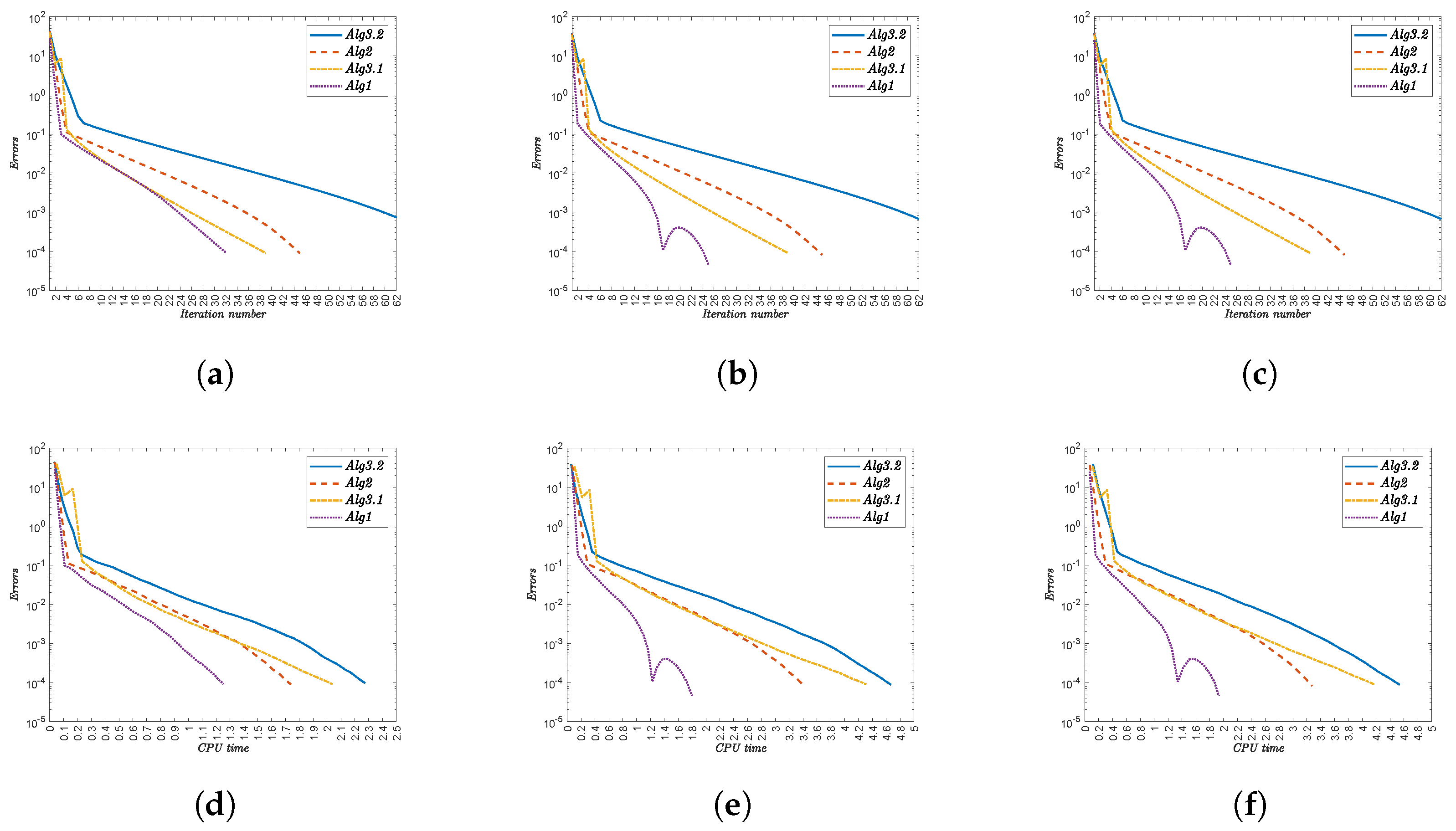
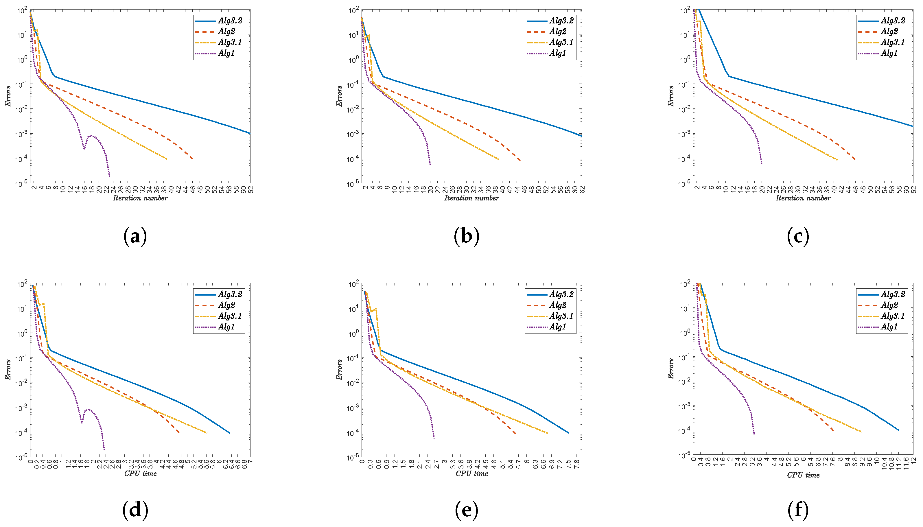
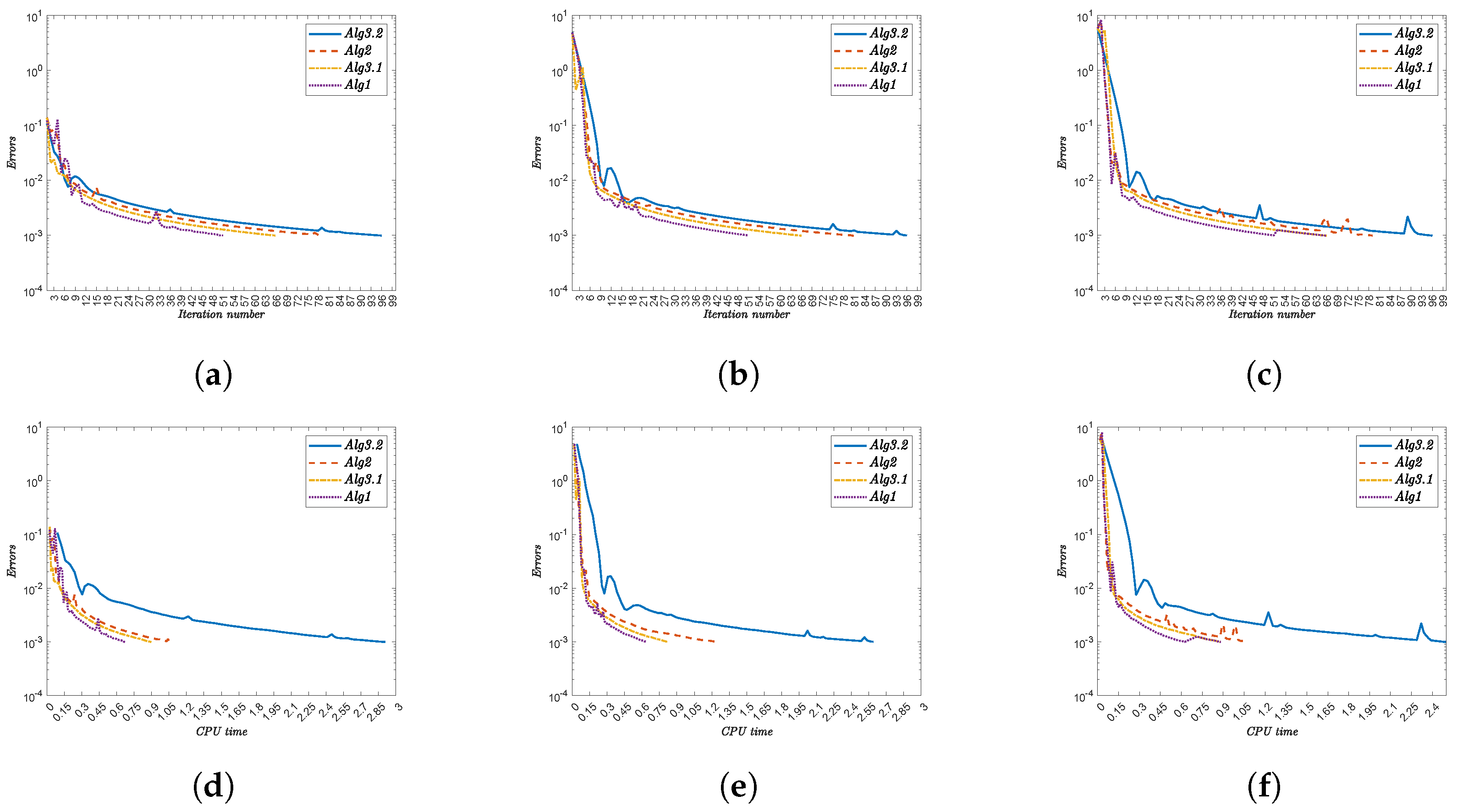
(i)

Alg1 demonstrates superior efficiency, consistently achieving the lowest iteration counts and CPU times. For instance,

• For x, Alg1 requires 32 iterations (1.225 s) versus Alg3.2’s 75 iterations (2.274 s).
• For $x^2\sin \left(x\right)$, Alg1 converges in 20 iterations (2.634 s), while Alg3.2 needs 76 iterations (7.542 s).

(ii)

The initial point $x_0$ significantly impacts convergence. Complex functions (e.g., $x^2\exp \left(x\right)\cos \left(x\right)$) amplify this effect, with Alg3.2 requiring 84 iterations (11.222 s) compared to Alg1’s 20 iterations (3.336 s).

(iii)

Nonlinearities in functions like $x^2\sin \left(x\right)$ increase computational demand, yet Alg1 maintains robust performance.

(iv)

The performance gap widens with function complexity, reinforcing Alg1’s scalability.

Alg1 outperforms competing algorithms across all test scenarios, demonstrating faster convergence and lower computational costs, particularly for complex functions. The results underscore its reliability for diverse optimization problems.

Example 3. 

The third example is adapted from [54], where the mapping $\mathcal{G}:{\mathbb{R}}^2\to {\mathbb{R}}^2$ is defined by

$$\mathcal{G}\left(u\right)=\left(\begin{array}{c}0.5u_1{u}_2-2u_2-{10}^7\\ -4u_1-0.1u_2^2-{10}^7\end{array}\right),$$

with the feasible set given by $\mathcal{C}=\{u\in {\mathbb{R}}^2\mid {(u_1-2)}^2+{(u_2-2)}^2\le 1\}$.

This mapping $\mathcal{G}$ satisfies several important properties. First, it is Lipschitz-continuous with Lipschitz constant $L=5$. Second, it is pseudomonotone on the set $\mathcal{C}$, though it is not monotone. Finally, the problem admits a unique solution, given by $u^{*}={(2.707,2.707)}^{\top }$.Parameter settings:

• Alg3.2 [38]: ${\lambda }_1=0.93$, $\theta =0.87$, $\mu =0.8$, ${\xi }_n={\left({\displaystyle \frac{2}{3n+2}}\right)}^2$, ${\psi }_n={\displaystyle \frac{2}{3n+2}}$, ${\kappa }_n={\displaystyle \frac{1-{\psi }_n}{2}}$, ${\varphi }_n={\displaystyle \frac{20}{{(2n+5)}^2}}$
• Alg2 [50]: ${\chi }_0=0.20$, $\mu =0.30$, $\theta =0.70$, ${\varphi }_n={\displaystyle \frac{1}{n+2}}$, ${\sigma }_n={\displaystyle \frac{1}{{(n+1)}^2}}$
• Alg3.1 [51]: ${\lambda }_0=0.5$, $\mu =0.4$, $\gamma =1.5$, ${\psi }_n={\displaystyle \frac{1}{n+1}}$, $p_n={\displaystyle \frac{1}{{(n+1)}^{1.1}}}$, $q_n={\displaystyle \frac{n+1}{n}}$, $\varphi =0.4$, ${\xi }_n={\displaystyle \frac{100}{{(n+1)}^2}}$
• Alg1 (Algorithm 1): ${\tau }_1=0.65$, ${\tau }_2=0.65$, ${\lambda }_1=0.45$, ${\psi }_n=0.7$, ${\beta }_n={\displaystyle \frac{1}{n+1}}$, ${\sigma }_{1,n}={\displaystyle \frac{100}{{(n+1)}^2}}$, ${\sigma }_{2,n}={\displaystyle \frac{100}{{(n+1)}^2}}$, $\delta =0.25$, ${\varphi }_n={\displaystyle \frac{20}{{(2n+5)}^2}}$

Comparative Numerical Analysis: This study conducts a systematic numerical comparison of four optimization algorithms—Alg1, Alg3.2, Alg2, and Alg3.1—evaluating their computational efficiency through iteration counts and CPU time. The analysis examines algorithm performance across multiple initial points $x_0\in {\mathbb{R}}^2$, including ${[1.5,1.7]}^{\top }$, ${[2.0,3.0]}^{\top }$, and others, to assess convergence behavior under varying starting conditions.

The numerical results, presented in Table 4 and Figure 5 and Figure 6, demonstrate that Alg1 consistently achieves superior performance. Notably, while iteration counts remain stable across different $x_0$ values, Alg1 maintains significantly lower computational times compared to competing methods. Key observations are as follows.

Table 4. Performance comparison across initial points $x_0$: iteration counts (n) and CPU times (t, seconds).

${\mathit{x}}_0$	Alg3.2		Alg2		Alg3.1		Alg1
	$\mathbf{n}$	$\mathbf{t}$	$\mathbf{n}$	$\mathbf{t}$	$\mathbf{n}$	$\mathbf{t}$	$\mathbf{n}$	$\mathbf{t}$
${[1.5,1.7]}^{\top }$	96	2.51503	80	1.05539	66	0.83240	51	0.69481
${[2.0,3.0]}^{\top }$	96	2.46246	79	1.12663	66	0.77810	51	0.62848
${[1.0,2.0]}^{\top }$	96	3.61541	80	1.50510	66	1.23019	51	0.96045
${[2.7,2.6]}^{\top }$	96	2.90826	79	1.06613	66	0.89569	51	0.67053
${[5.0,3.0]}^{\top }$	96	2.59047	81	1.25559	66	0.82584	51	0.63624
${[4.0,6.0]}^{\top }$	96	2.49513	79	1.07621	66	0.88292	51	0.63624

Figure 5. Convergence behavior of Alg3.2, Alg2, Alg3.1, and Alg1 for different initial points. The top row shows error versus iteration count; the bottom row shows error versus CPU time. (a) Error vs. iteration for $x_0={[1.5,1.7]}^{\top }$. (b) Error vs. iteration for $x_0={[2.0,3.0]}^{\top }$. (c) Error vs. iteration for $x_0={[1.0,2.0]}^{\top }$. (d) Error vs. time for $x_0={[1.5,1.7]}^{\top }$. (e) Error vs. time for $x_0={[2.0,3.0]}^{\top }$. (f) Error vs. time for $x_0={[1.0,2.0]}^{\top }$.

Figure 6. Convergence behavior for additional initial points. Top row: error versus iteration count; bottom row: error versus CPU time. Algorithms compared: Alg3.2, Alg2, Alg3.1, and Alg1. (a) Error vs. iteration for $x_0={[2.7,2.6]}^{\top }$. (b) Error vs. iteration for $x_0={[5.0,3.0]}^{\top }$. (c) Error vs. iteration for $x_0={[4.0,6.0]}^{\top }$. (d) Error vs. time for $x_0={[2.7,2.6]}^{\top }$. (e) Error vs. time for $x_0={[5.0,3.0]}^{\top }$. (f) Error vs. time for $x_0={[4.0,6.0]}^{\top }$.

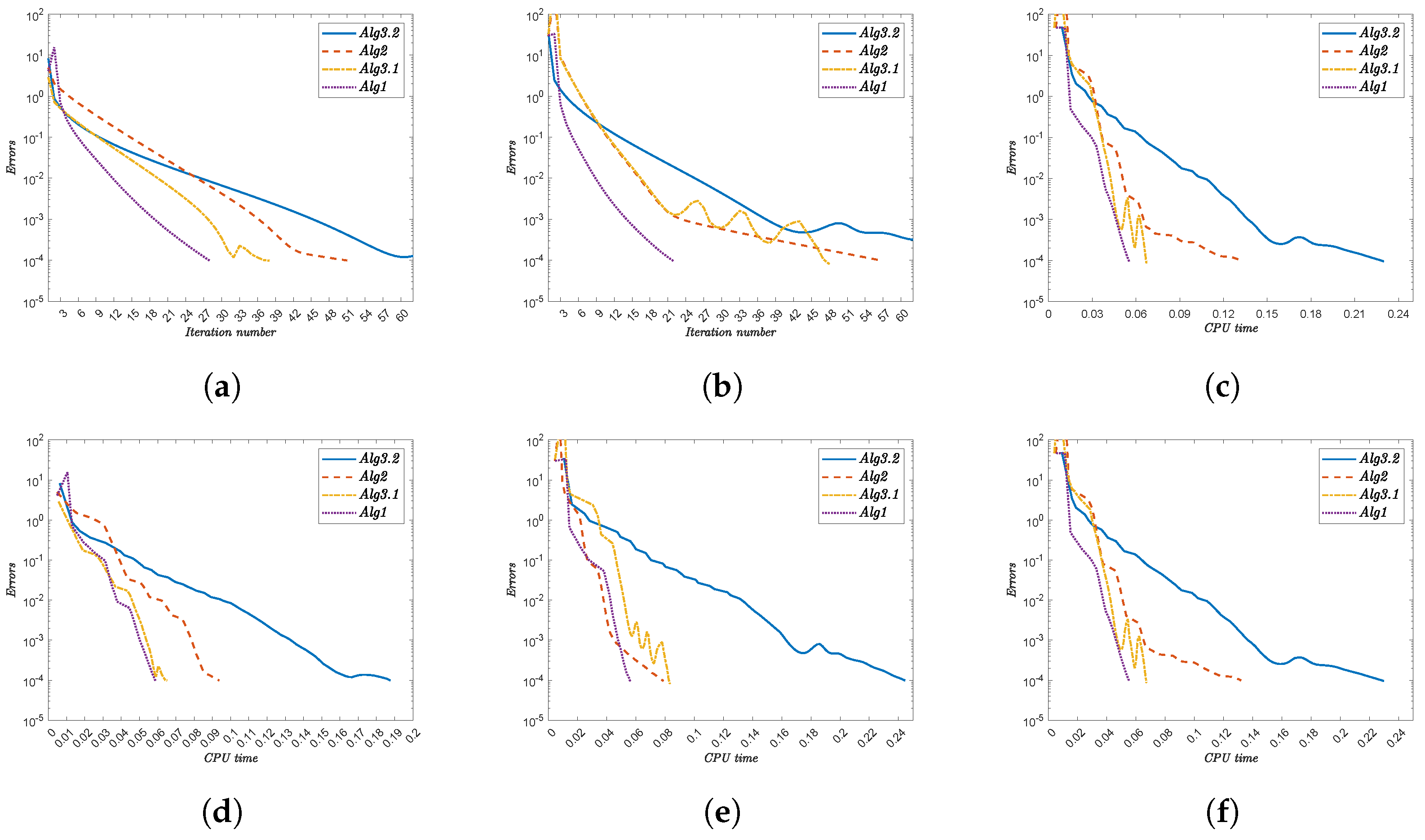
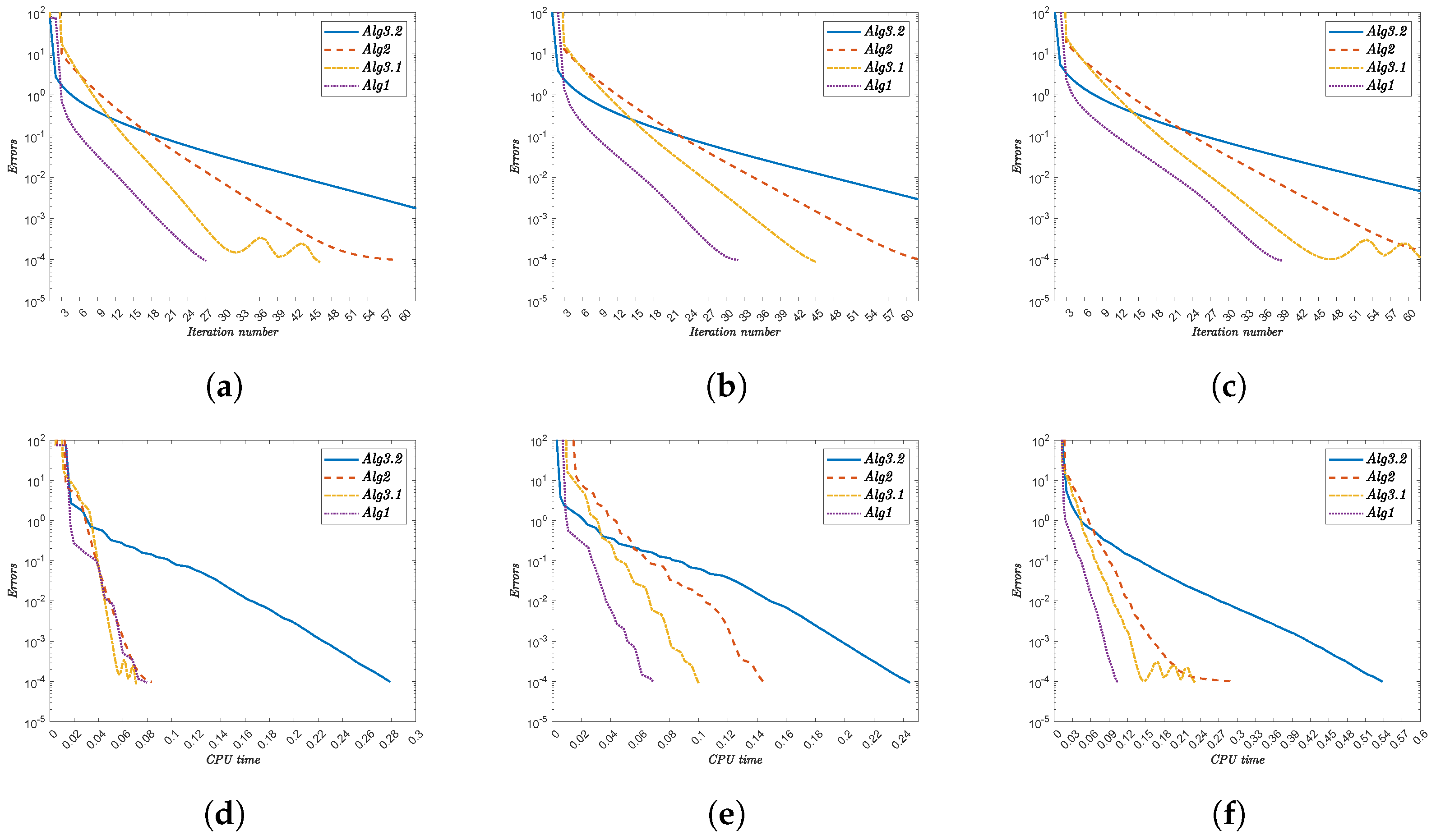
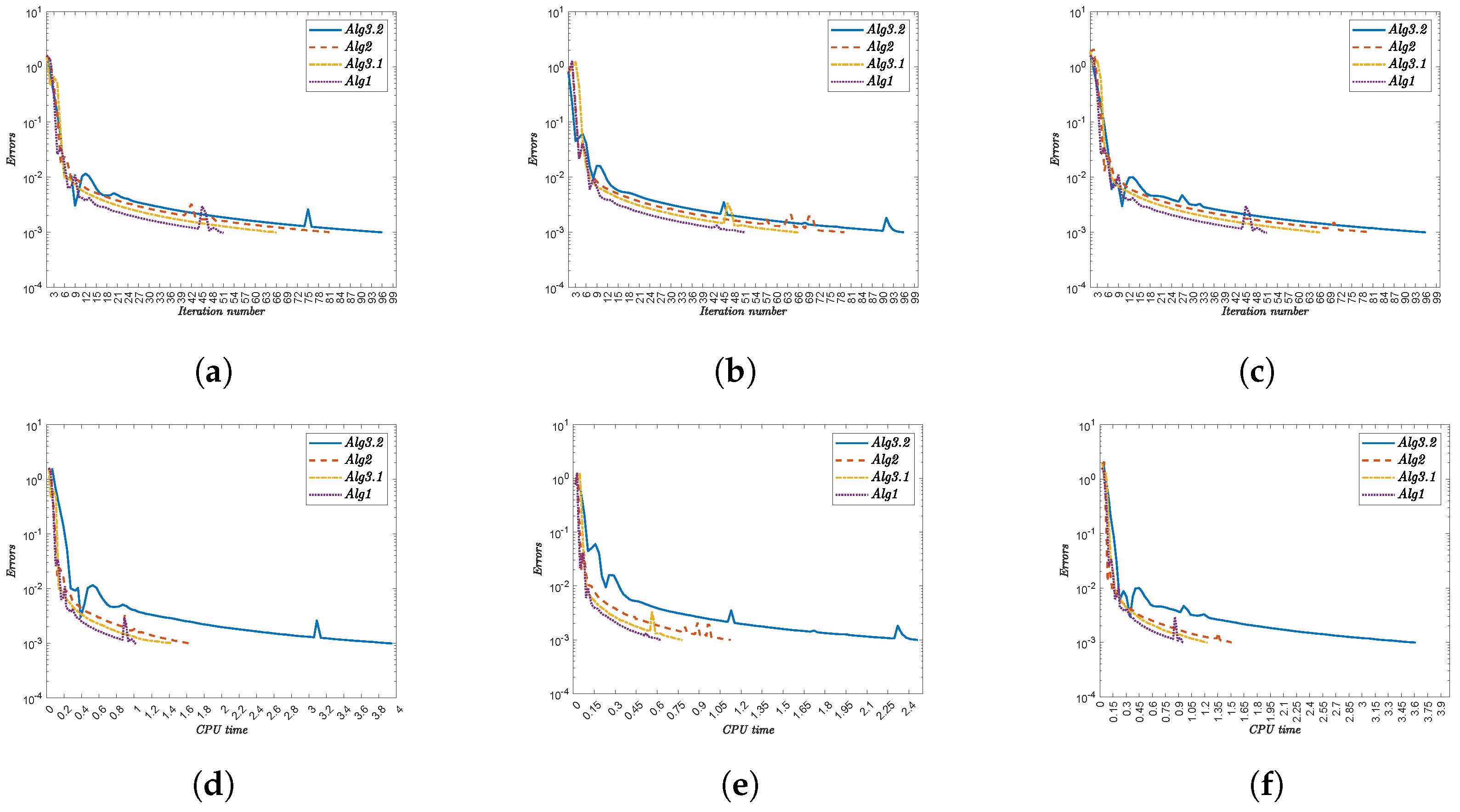
(i)

Alg1 outperforms all other algorithms in both metrics. For $x_0={[1.5,1.7]}^{\top }$, it completes in 51 iterations (0.69481 s) versus Alg3.2’s 96 iterations (2.51503 s).

(ii)

The performance advantage persists across all test cases. At $x_0={[2.0,3.0]}^{\top }$, Alg1 requires 51 iterations (0.62848 s) compared to Alg3.2’s 96 iterations (2.46246 s).

(iii)

Iteration counts remain constant for each algorithm regardless of $x_0$:

• Alg3.2: 96 iterations.
• Alg2: 79–81 iterations.
• Alg3.1: 66 iterations.
• Alg1: 51 iterations.

(iv)

CPU times show minor variations with $x_0$. For Alg1, they range from 0.62848 s (${[2.0,3.0]}^{\top }$) to 0.96045 s (${[1.0,2.0]}^{\top }$).

(v)

The computational advantage of Alg1 is most pronounced against Alg3.2. At $x_0={[2.7,2.6]}^{\top }$, Alg1 uses 0.67053 s versus Alg3.2’s 2.90826 s.

(vi)

Alg1 demonstrates robust efficiency across all test cases, maintaining low CPU times without compromising convergence speed.

Alg1 emerges as the most efficient algorithm, demonstrating consistent superiority in both iteration counts and computational time across all tested initial points $x_0$. The results highlight its robustness and practical value for optimization tasks.

5. Conclusions and Future Directions

This study introduces a novel algorithm for solving variational inequality problems in real Hilbert spaces, which is particularly effective for equilibrium problems involving monotone operators. The algorithm’s key innovation is its dynamic variable step size mechanism, which provides two significant advantages: first, it eliminates the need for prior knowledge of Lipschitz-type constants, and second, it avoids the computational overhead associated with line search procedures. Extensive numerical experiments demonstrate the algorithm’s superior performance compared to existing methods in the literature.

Future Research Directions

The promising results suggest several valuable extensions for future work.

1. Application to problems with non-monotone or quasi-monotone operators, which would expand the algorithm’s practical utility across a wider range of problems.

2. Extensions to handle equilibrium problems with additional constraints, such as composite or split feasibility constraints, enabling solutions to more complex optimization scenarios.

3. The development of parallel and distributed implementations to enhance computational efficiency, particularly for large-scale problems in high-dimensional spaces.

4. Further theoretical analysis to establish convergence under weaker or more general conditions, thereby broadening the algorithm’s applicability.

5. Practical applications in important domains, including image reconstruction, machine learning, and network optimization, to validate and demonstrate the method’s effectiveness in real-world settings.

6. Exploration of alternative dynamic step size strategies, potentially incorporating adaptive learning or machine learning techniques, to further improve convergence speed and robustness.

References

- Alakoya, T.O.; Mewomo, O.T. Viscosity s-iteration method with inertial technique and self-adaptive step size for split variational inclusion, equilibrium and fixed point problems. Comput. Appl. Math. 2022, 41, 31–39. [Google Scholar] [CrossRef]
- Aubin, J.-P.; Ekeland, I. Applied Nonlinear Analysis; Wiley: Hoboken, NJ, USA, 1984. [Google Scholar]
- Ogwo, G.N.; Izuchukwu, C.; Shehu, Y.; Mewomo, O.T. Convergence of relaxed inertial subgradient extragradient methods for quasimonotone variational inequality problems. J. Sci. Comput. 2022, 90, 35. [Google Scholar] [CrossRef]
- Baiocchi, C.; Capelo, A. Variational and Quasivariational Inequalities: Applications to Free Boundary Problems; Wiley: Hoboken, NJ, USA, 1984. [Google Scholar]
- Censor, Y.; Gibali, A.; Reich, S. Algorithms for the split variational inequality problem. Numer. Algorithms 2012, 59, 301–323. [Google Scholar] [CrossRef]
- Godwin, E.C.; Mewomo, O.T.; Alakoya, T.O. A strongly convergent algorithm for solving multiple set split equality equilibrium and fixed point problems in Banach spaces. Proc. Edinb. Math. Soc. 2023, 66, 475–515. [Google Scholar] [CrossRef]
- Kinderlehrer, D.; Stampacchia, G. An Introduction to Variational Inequalities and Their Applications; SIAM: Philadelphia, PA, USA, 2000. [Google Scholar]
- Geunes, J.; Pardalos, P.M. Network optimization in supply chain management and financial engineering: An annotated bibliography. Networks 2003, 42, 66–84. [Google Scholar] [CrossRef]
- Nagurney, A. Network Economics: A Variational Inequality Approach, 2nd ed.; Kluwer Academic Publishers: Dordrecht, The Netherlands, 1999. [Google Scholar]
- Nagurney, A.; Dong, J. Supernetworks: Decision-Making for the Information Age; Edward Elgar Publishing: Northampton, MA, USA, 2002. [Google Scholar]
- Smith, M.J. The existence, uniqueness and stability of traffic equilibria. Transp. Res. B 1979, 13, 295–304. [Google Scholar] [CrossRef]
- Dafermos, S. Traffic equilibrium and variational inequalities. Transp. Sci. 1980, 14, 42–54. [Google Scholar] [CrossRef]
- Lawphongpanich, S.; Hearn, D.W. Simplicial decomposition of the asymmetric traffic assignment problem. Transp. Res. B 1984, 18, 123–133. [Google Scholar] [CrossRef]
- Panicucci, B.; Pappalardo, M.; Passacantando, M. A path-based double projection method for solving the asymmetric traffic network equilibrium problem. Optim. Lett. 2007, 1, 171–185. [Google Scholar] [CrossRef]
- Aussel, D.; Gupta, R.; Mehra, A. Evolutionary variational inequality formulation of the generalized Nash equilibrium problem. J. Optim. Theory Appl. 2016, 169, 74–90. [Google Scholar] [CrossRef]
- Ciarciá, C.; Daniele, P. New existence Theorems for quasi-variational inequalities and applications to financial models. Eur. J. Oper. Res. 2016, 251, 288–299. [Google Scholar] [CrossRef]
- Nagurney, A.; Parkes, D.; Daniele, P. The internet, evolutionary variational inequalities, and the time-dependent Braess paradox. Comput. Manag. Sci. 2007, 4, 355–375. [Google Scholar] [CrossRef]
- Scrimali, L.; Mirabella, C. Cooperation in pollution control problems via evolutionary variational inequalities. J. Glob. Optim. 2018, 70, 455–476. [Google Scholar] [CrossRef]
- Xu, S.; Li, S. A strongly convergent alternated inertial algorithm for solving equilibrium problems. J. Optim. Theory Appl. 2025, 206, 35. [Google Scholar] [CrossRef]
- Yao, Y.; Adamu, A.; Shehu, Y. Strongly convergent golden ratio algorithms for variational inequalities. Math. Methods Oper. Res. 2025. [Google Scholar] [CrossRef]
- Tan, B.; Qin, X. Two relaxed inertial forward-backward-forward algorithms for solving monotone inclusions and an application to compressed sensing. Can. J. Math. 2025, 1–22. [Google Scholar] [CrossRef]
- Argyros, I.K. The Theory and Applications of Iteration Methods, 2nd ed.; CRC Press: Boca Raton, FL, USA, 2022. [Google Scholar]
- Korpelevich, G.M. The extragradient method for finding saddle points and other problems. Ekonom. Mat. Methods 1976, 12, 747–756. [Google Scholar]
- Tseng, P. A modified forward-backward splitting method for maximal monotone mappings. SIAM J. Control Optim. 2000, 38, 431–446. [Google Scholar] [CrossRef]
- Thong, D.V.; Hieu, D.V. Modified subgradient extragradient method for variational inequality problems. Numer. Algorithms 2018, 79, 597–610. [Google Scholar] [CrossRef]
- Reich, S.; Thong, D.V.; Cholamjiak, P.; Long, L.V. Inertial projection-type methods for solving pseudomonotone variational inequality problems in Hilbert space. Numer. Algorithms 2021, 88, 813–835. [Google Scholar] [CrossRef]
- Suleiman, Y.I.; Kumam, P.; Rehman, H.U.; Kumam, W. A new extragradient algorithm with adaptive step-size for solving split equilibrium problems. J. Inequal. Appl. 2021, 2021, 136. [Google Scholar] [CrossRef]
- Rehman, H.U.; Tan, B.; Yao, J.C. Relaxed inertial subgradient extragradient methods for equilibrium problems in Hilbert spaces and their applications to image restoration. Commun. Nonlinear Sci. Numer. Simul. 2025, 146, 108795. [Google Scholar] [CrossRef]
- Ceng, L.C.; Ghosh, D.; Rehman, H.U.; Zhao, X. Composite Tseng-type extragradient algorithms with adaptive inertial correction strategy for solving bilevel split pseudomonotone VIP under split common fixed-point constraint. J. Comput. Appl. Math. 2025, 470, 116683. [Google Scholar] [CrossRef]
- Nwawuru, F.O.; Ezeora, J.N.; Rehman, H.U.; Yao, J.C. Self-adaptive subgradient extragradient algorithm for solving equilibrium and fixed point problems in Hilbert spaces. Numer. Algorithms 2025. [Google Scholar] [CrossRef]
- Dong, Q.; Cho, Y.; Zhong, L.; Rassias, T.M. Inertial projection and contraction algorithms for variational inequalities. J. Glob. Optim. 2018, 70, 687–704. [Google Scholar] [CrossRef]
- Solodov, M.V.; Svaiter, B.F. A new projection method for variational inequality problems. SIAM J. Control Optim. 1999, 37, 765–776. [Google Scholar] [CrossRef]
- Censor, Y.; Gibali, A.; Reich, S. The subgradient extragradient method for solving variational inequalities in Hilbert space. J. Optim. Theory Appl. 2011, 148, 318–335. [Google Scholar] [CrossRef]
- Censor, Y.; Gibali, A.; Reich, S. Extensions of Korpelevich’s extragradient method for the variational inequality problem in Euclidean space. Optimization 2012, 61, 1119–1132. [Google Scholar] [CrossRef]
- Polyak, B.T. Some methods of speeding up the convergence of iterative methods. USSR Comput. Math. Math. Phys. 1964, 4, 1–17. [Google Scholar] [CrossRef]
- Gibali, A.; Jolaoso, L.O.; Mewomo, O.T.; Taiwo, A. Fast and simple Bregman projection methods for solving variational inequalities and related problems in Banach spaces. Results Math. 2020, 75, 179. [Google Scholar] [CrossRef]
- Godwin, E.C.; Alakoya, T.O.; Mewomo, O.T.; Yao, J.-C. Relaxed inertial Tseng extragradient method for variational inequality and fixed point problems. Appl. Anal. 2023, 102, 4253–4278. [Google Scholar] [CrossRef]
- Alakoya, T.O.; Mewomo, O.T. Strong convergent inertial two-subgradient extragradient method for finding minimum-norm solutions of variational inequality problems. Netw. Spat. Econ. 2024, 24, 425–459. [Google Scholar] [CrossRef]
- Yao, Y.H.; Iyiola, O.S.; Shehu, Y. Subgradient extragradient method with double inertial steps for variational inequalities. J. Sci. Comput. 2022, 90, 71. [Google Scholar] [CrossRef]
- Thong, D.V.; Dung, V.T.; Anh, P.K.; Van Thang, H. A single projection algorithm with double inertial extrapolation steps for solving pseudomonotone variational inequalities in Hilbert space. J. Comput. Appl. Math. 2023, 426, 115099. [Google Scholar] [CrossRef]
- Li, H.; Wang, X. Subgradient extragradient method with double inertial steps for quasi-monotone variational inequalities. Filomat 2023, 37, 9823–9844. [Google Scholar] [CrossRef]
- Pakkaranang, N. Double inertial extragradient algorithms for solving variational inequality problems with convergence analysis. Math. Methods Appl. Sci. 2024, 47, 11642–11669. [Google Scholar] [CrossRef]
- Wang, K.; Wang, Y.; Iyiola, O.S.; Shehu, Y. Double inertial projection method for variational inequalities with quasi-monotonicity. Optimization 2024, 73, 707–739. [Google Scholar] [CrossRef]
- Bauschke, H.H.; Combettes, P.L. Convex Analysis and Monotone Operator Theory in Hilbert Spaces, 2nd ed.; Springer: Berlin/Heidelberg, Germany, 2017. [Google Scholar]
- Bianchi, M.; Schaible, G. Generalized monotone bifunctions and equilibrium problems. J. Optim. Theory Appl. 1996, 90, 31–43. [Google Scholar] [CrossRef]
- Bauschke, H.H.; Combettes, P.L. A weak-to-strong convergence principle for Fejér-monotone methods in Hilbert spaces. Math. Oper. Res. 2001, 26, 248–264. [Google Scholar] [CrossRef]
- He, S.; Xu, H.-K. Uniqueness of supporting hyperplanes and an alternative to solutions of variational inequalities. J. Glob. Optim. 2013, 57, 1375–1384. [Google Scholar] [CrossRef]
- Saejung, G.; Yotkaew, P. Approximation of zeros of inverse strongly monotone operators in Banach spaces. Nonlinear Anal. Theory Methods Appl. 2012, 75, 742–750. [Google Scholar] [CrossRef]
- Tan, K.K.; Xu, H.-K. Approximating fixed points of nonexpansive mappings by the Ishikawa iteration process. J. Math. Anal. Appl. 1993, 178, 301–308. [Google Scholar] [CrossRef]
- Muangchoo, K.; Alreshidi, N.A.; Argyros, I.K. Approximation results for variational inequalities involving pseudomonotone bifunction in real Hilbert spaces. Symmetry 2021, 13, 182. [Google Scholar] [CrossRef]
- Tan, B.; Sunthrayuth, P.; Cholamjiak, P.; Cho, Y.J. Modified inertial extragradient methods for finding minimum-norm solution of the variational inequality problem with applications to optimal control problem. Int. J. Comput. Math. 2023, 100, 525–545. [Google Scholar] [CrossRef]
- Harker, P.T.; Pang, J.S. For the linear complementarity problem. Lect. Appl. Math. 1990, 26, 265–284. [Google Scholar]
- Van Hieu, D.; Anh, P.K.; Muu, L.D. Modified hybrid projection methods for finding common solutions to variational inequality problems. Comput. Optim. Appl. 2017, 66, 75–96. [Google Scholar] [CrossRef]
- Shehu, Y.; Dong, Q.L.; Jiang, D. Single projection method for pseudo-monotone variational inequality in Hilbert spaces. Optimization 2018, 68, 385–409. [Google Scholar] [CrossRef]