Article

Predictive Analysis of Carbon Emissions in China’s Construction Industry Based on GIOWA Model

College of Information Management, Nanjing Agricultural University, Nanjing 211800, China
*
Author to whom correspondence should be addressed.
Mathematics 2025, 13(12), 1955; https://doi.org/10.3390/math13121955
Submission received: 9 May 2025 / Revised: 9 June 2025 / Accepted: 10 June 2025 / Published: 13 June 2025

Abstract

The construction industry in China has long been confronted with significant concerns related to fossil fuel dependence and low energy efficiency. However, under the policy guidance of China’s “dual carbon” goals, it has emerged as the leading sector in achieving a reduction in carbon emissions through technological innovation in recent years. To accurately assess the carbon emission reduction potential of the construction industry and support the attainment of the dual carbon goals, this study constructs a generalized induced ordered weighted averaging (GIOWA) combination forecasting model, integrating support vector regression (SVR) and a long short-term memory neural network (LSTM). A case study is conducted based on historical data (1997–2021) from the construction industry, and the research findings indicate that: (1) the GIOWA combination forecasting model effectively integrates the algorithmic strengths of SVR and LSTM, achieving an average prediction accuracy of 98.16%, which signifies a remarkable improvement over both individual models; (2) the carbon emissions in China’s construction industry will maintain a downward trend during the period 2022–2030, although the decline rate is expected to decrease gradually; (3) by 2030, a reduction of nearly 35% in carbon emissions is anticipated relative to the historical peak. This study provides evidence-based decision support for relevant policy formulation.

1. Introduction

As the issue of global climate change intensifies, increasing carbon emissions have become a shared concern for the international community. In this context, numerous nations have implemented proactive strategies to address relevant issues. Among developed countries, the United States has proposed the Clean Competition Act (CCA), which aims to reduce environmental pollution while facilitating the adoption of cleaner production methods for domestic manufacturing [1]. The European Union initiated the Carbon Border Adjustment Mechanism (CBAM) in 2023 to promote carbon emission reduction via strategic policy measures [2]. As a leading advocate for the Paris Agreement, China issued dual carbon goals in 2020, with the aim of achieving carbon peaking by 2030 and realizing carbon neutrality by 2060 [3]. These goals are designed to drive a green transformation across various industries, thereby enhancing China’s contribution to global climate governance. Specifically, the construction industry in China plays a vital role in fostering economic growth and job creation. However, it has long been confronted with intensive fossil fuel consumption and low energy utilization efficiency during the construction process. Notably, while carbon emissions from the manufacturing, transportation, and energy sectors continue to rise, the construction industry has emerged as the leading sector to exhibit a downward trend in carbon emissions [4,5,6,7]. Therefore, precise and robust prediction is essential to accurately evaluate the carbon emission reduction potential of China’s construction industry, which can provide a scientific basis for relevant policy formulation.
In recent years, the issue of carbon emission forecasting has attracted significant interest from academics. Depending on the features and structure of the dataset, the forecasting methods can be generally divided into two categories: influential factor forecasting and time series forecasting [8].
The objective of influential factor forecasting is to develop a mathematical framework that identifies and quantifies the key factors significantly associated with the target variable, thereby simulating the collaborative influence of multiple factors in real-world contexts and enabling accurate predictions. Consequently, numerous studies have focused on the rational selection of influential factors. In 1971, Ehrlich and Holdren first introduced the IPAT model, which linked environmental pressure (I) to three key factors: population (P), affluence (A), and technology (T) [9]. This model established a foundational framework for examining the environmental impacts of human activities. On this basis, the Kaya identity effectively eliminates residual terms resulting from the decomposition process, while providing a sharper focus on carbon emission analysis [10]. However, both the IPAT model and the Kaya identity overlook the nonlinear relationship between the influential factors and the target variable, thus failing to characterize the evolving trajectories of carbon emissions. To overcome these limitations, the STIRPAT model was proposed by Dietz and Rosa in 1997 [11]. This model quantifies the sensitivity of carbon emissions to influential factors by introducing the elasticity coefficient, thereby enhancing the reliability of the prediction result. In addition, due to its superior scalability, it has been widely adopted across various industries, including construction [12,13,14], logistics [15,16,17], power [18,19], etc., and is progressively becoming the mainstream. However, the introduction of multiple influential factors complicates the data collection process, and the increasing complexity of the model presents a new challenge for enhancing the prediction accuracy.
Time series forecasting analyzes the chronological order and underlying patterns within the sample data, enabling predictions through a trend extrapolation process. Early time series forecasting models are primarily developed based on statistical theories, including the Exponential Smoothing (ES) model [20,21], the Grey Model (GM) [22,23,24], and the Autoregressive Integrated Moving Average (ARIMA) model [25,26,27]. However, the prevalent limitations of these models stems from their restrictive assumptions about the stationarity and linearity of the data. Such constraints can result in reduced prediction accuracy when dealing with nonlinear time series. As machine learning algorithms advance, numerous researchers have sought to utilize their superior capability in handling nonlinear data [28,29,30,31]. Ahmed A. A. et al. proposed a novel model based on nonlinear Gaussian Process Regression (GPR), attaining an R2 of up to 98.1%, significantly outperforming the traditional models [32]. Chen et al. developed an improved BPNN model for predicting greenhouse gas emissions, achieving R2 values exceeding 99%, which provides theoretical support for optimizing engine emission control strategies [33]. In recent years, deep learning has emerged as a vital branch in machine learning, demonstrating its robust ability to characterize complex patterns and features through multi-layer neural network architectures. Remarkably, this trait is essential for capturing long-term dependencies within the carbon emission data and enabling accurate predictions. Kumari, S. and Singh, S. K. employed multiple machine learning techniques to analyze carbon dioxide emissions in India, revealing that the deep learning model LSTM performed optimally in terms of prediction accuracy and robustness [34]. Shakhovska et al. integrated the strengths of FractalNet [35] in multi-scale feature extraction with the robust sequence modeling capabilities of LSTM to propose the FractalNet-LSTM model [36]. The results highlight the model’s exceptional efficacy in dealing with data characterized by long-term and cyclical dependencies. Notably, time series forecasting models operate under the assumption that the historical data of the target variable encompasses all the relevant information influencing the forecast value [37]. However, carbon emissions in the construction industry are susceptible to uncertain factors, including environmental policy adjustments. Therefore, the achievement of precise prediction results cannot solely depend on the target variable data while ignoring the information contained in the key influential factors.
The above analysis indicates that both influential factor forecasting and time series forecasting models possess intrinsic limitations. To overcome the deficit of individual prediction models and achieve more accurate and robust forecast results, the development of combination forecasting models has emerged as a crucial focus in contemporary research. Based on distinct weight determination methods, they can be classified into two categories: fixed-weight combination forecasting and variable-weight combination forecasting. Fixed-weight combination forecasting is characterized by the assignment of constant weights to each constituent model. Representative models in this category include equal weighting [38,39], Markowitz mean-variance optimization [40,41,42], and regression-based weighted averaging [43]. However, as forecasting methodologies evolve and application contexts grow more intricate, the shortcomings of fixed-weight models have become increasingly evident. Most critically, the fixed-weight setting leads to poor dynamic adaptability when forecasting uncertain factors such as carbon emissions [44]. In order to rectify this deficiency, variable-weight combination forecasting models have been developed. The core idea of these models is dynamically weighting individual models according to temporal discrepancies in their predictive performance. Since Yager initially proposed the ordered weighted averaging (OWA) operator in 1988 [45], academia has successively advanced various improved operators: induced ordered weighted arithmetic averaging (IOWA) [46,47], induced ordered weighted geometric averaging (IOWGA) [48,49,50], induced ordered weighted harmonic averaging (IOWHA) [51,52], and generalized induced ordered weighted averaging (GIOWA) [53]. Variable-weight models embedded with these operators have demonstrated effective results in predicting the characteristics of complex systems. Notably, the GIOWA operator integrates the advantages of various operators while introducing a generalization mechanism through parameterized extensions. Thus, the forecasting model based on the GIOWA operator allows for more effective handling of the uncertainties arising from policy interventions and other factors. This study employs the GIOWA operator to construct a variable-weight forecasting model, aiming to enhance the prediction accuracy of carbon emissions in China’s construction industry and provide evidence-based decision support for policy formulation.

2. Methodology

2.1. GIOWA Combination Forecasting Model

Suppose that the n-dimensional sequence { x i , i = 1 ,   2 , , n } and the corresponding induced variable sequence { α i , i = 1,2 , , n } can be combined into n ordered pairs α 1 , x 1 , α 2 , x 2 , , α n , x n , α i 0 , i = 1,2 , , n . Let W = ( w 1 , w 2 , , w n ) T be the weight vector that satisfies the condition i = 1 n w i = 1 , w i 0 . Then the general form of the GIOWA operator is defined as follows:
G I O W A W α 1 , x 1 ,   α 2 , x 2 ,   ,   α n , x n = i = 1 n w i x α i n d e x i λ 1 / λ λ 0
where α i n d e x i represents the index of the i-th largest number in the sequence { α i } and λ is the averaging exponent. This indexing method enables the weight coefficient w i to be combined with the ordered sequence x α i n d e x i , thereby completing the induced ordering process.
Specifically, as for forecasting problems, prediction accuracy can serve as the induced variable α . At each period t, multiple forecasts are ranked and recombined to generate sequences ordered by their accuracy, such as the most accurate sequence, the second most accurate sequence, and so on.
Let x t denote the actual carbon emissions of the construction industry at period t, and x i t represent the forecast result of the i-th individual model of the same period. Therefore, the combination forecasting result can be expressed as x ^ t = i = 1 n w i x i t . On this basis, assuming that α i t   ( i = 1,2 , , n ; t = 1,2 , , N ) denotes the prediction accuracy of the i-th individual model at period t, then it can be calculated as follows:
α i t = 1 x t x i t x t , x t x i t x t 1 0   , x t x i t x t > 1
After the induced ordering process, the GIOWA combination forecasting result is as follows:
x ^ t = i = 1 n w i x α i n d e x i t λ 1 / λ λ 0
where α i n d e x ( i t ) is the number of the i-th accurate individual model at period t, and x α i n d e x ( i t ) λ denotes the λ-th power of the corresponding prediction result. Figure 1 illustrates the process of induced ordering in the GIOWA combination forecasting model. The core idea of the GIOWA model is dynamically assigning descending weights to different models according to their predictive performance, thereby optimizing the overall accuracy.
Notably, by adjusting the value of λ, the GIOWA model evolves into distinct sub-models, with typical examples as follows:
(1) When λ = 1, the corresponding model is the IOWA combination forecasting model, with the formula:
x ^ t = i = 1 n w i x α i n d e x i t
(2) When λ approaches 0, the GIOWA model becomes the IOWGA combination forecasting model, expressed as follows:
x ^ t = i = 1 n x α i n d e x i t w i
(3) When λ = −1, the original model transforms into the IOWHA combination forecasting model, given by the following:
x ^ t = i = 1 n w i x α i n d e x i t 1
In addition to the induced ordering process, the utilization of error information is another key aspect of the GIOWA model, as it is closely correlated with the determination of the optimal combination weights. Let r α i n d e x ( i t ) = x t λ x α i n d e x i t λ denote the λ-th power of the induced prediction error of the i-th accurate individual model at period t. Based on Equation (3), the λ-th power of prediction error in GIOWA model can be expressed as follows:
x t λ x ^ t λ = x t λ i = 1 n w i x α i n d e x i t λ = i = 1 n w i x t λ i = 1 n w i x α i n d e x i t λ = i = 1 n w i x t λ x α i n d e x i t λ = i = 1 n w i r α i n d e x i t
Equation (7) calculates the λ-th power prediction error at period t, whereas the model’s forecasting efficacy is evaluated by the cumulative deviation over the sample period N. Therefore, the sum of squared errors (SSE) is employed as a metric for measuring forecasting performance, and the corresponding formula is as follows:
S = t = 1 N x t λ x ^ t λ 2 = t = 1 N i = 1 n w i r α i n d e x i t 2 = i = 1 n j = 1 n w i w j t = 1 N r α i n d e x i t r α i n d e x j t = i = 1 n j = 1 n w i w j R i j = W T R W
where S represents the SSE, R = ( R i j ) n × n is called the λ-th power error information matrix, and W denotes the combination weight vector to be optimized.
Based on the above analysis, the optimization model that minimizes the SSE over the sample period can be expressed as Equation (9). Here, u n represents the n-dimensional unit column vector.
min S = W T R W s . t . u n T W = 1 W 0
where u n denotes the n-dimensional unit column vector. The optimization is performed with respect to the weight vector W .
Adopting the SSE as the objective function simplifies the model structure to a quadratic programming formulation. This enables most solvers to quickly complete the computation task, thus enhancing the practicality of the GIOWA combination forecasting model in determining optimal weights.
Notably, although the weight coefficients derived from Equation (9) remain constant across different periods, the GIOWA model is fundamentally a variable-weight combination forecasting model. As indicated by Equation (3), the weight coefficients are combined with the sequences ordered by prediction accuracy. This implies that the individual model x i t varies across different periods, even though it is associated with the same weight coefficient w i . Therefore, it is the induced ordering process that endows the GIOWA model with the characteristic of time-varying weights, thereby enhancing its flexibility in addressing uncertainties compared with traditional fixed-weight models.
The GIOWA combination forecasting model effectively integrates the algorithmic strengths of various individual models to improve forecast performance. However, selecting component models with high forecast accuracy remains an essential prerequisite in practical applications.

2.2. Individual Forecasting Models

2.2.1. Support Vector Regression Model

The Support Vector Regression (SVR) model is widely applied in the fields of influential factor forecasting, especially for nonlinear and small-sample data. Its core concept is to maximize the margin between the data points and the hyperplane in a high-dimensional feature space, thereby identifying an optimal decision boundary that allows for a certain error tolerance. This strategy facilitates precise regression prediction while preserving the model’s generalization capability. Given that the carbon emissions in the construction industry are intricately linked to multiple influential factors such as population, economy, and technology [54], this study utilizes the SVR model to analyze and depict the evolving dynamics between carbon emissions and their associated factors.
The standard form of the ε -SVR model can be formulated as follows:
min ω , ξ   1 2 ω 2 + C i = 1 n ξ i + ξ i s . t . f x i y i ε + ξ i y i f x i ε + ξ i ξ i 0 , ξ i 0 , i = 1,2 , , n
where ω denotes the coefficient vector of the hyperplane. ω denotes the Euclidean norm of ω , which is used to calculate the magnitude of it. C represents the penalty parameter, while ξ i and ξ i are utilized as the slack variables. Specifically, the first term in Equation (10) directly affects the fitting capability of the model, while the second term, which serves as a regularization component, ensures robustness against the noise, thereby preventing overfitting and enhancing the generalization performance.
Lagrange multipliers α i ,   α i ,   η i , and η i are introduced to construct the Lagrangian function:
L ω , b , ξ , ξ , α , α , η , η = 1 2 ω 2 + C i = 1 n ξ i + ξ i i = 1 n α i f ( x i ) y i ε ξ i i = 1 n α i y i f ( x i ) ε ξ i i = 1 n η i ξ i i = 1 n η i ξ i
By calculating the partial derivatives of this function for ω , b , ξ , ξ and setting them to zero, the corresponding dual problem is obtained as follows:
max α , α   { 1 2 i , j = 1 n α i α i α j α j x i , x j + ε i = 1 n α i + α i i = 1 n y i α i α i } s . t . i = 1 n ( α i α i ) = 0 0 α i , α i C ( i = 1,2 , , n )
Notably, although η i and η i do not explicitly appear in the final dual problem, they are utilized in the differentiation process to ensure that α i and α i satisfy the constraints α i C and α i C .
Additionally, the kernel function is employed to implicitly map the original data into a high-dimensional space. This transformation turns the problem into the search for a linear regression model, thereby avoiding complex calculations. The resulting regression equation is given by the following:
f x = i = 1 n α i α i K ( x i , x ) + b
where K ( x i , x ) represents the kernel function, and the Gaussian Radial Basis Function (RBF) is utilized in this study, with its formula provided below:
K x i , x = e x p | | x x i | | 2 2 σ 2
where x x i denotes the Euclidean norm of the vector difference x x i .
Based on the above analysis, the SVR model characterizes the nonlinear relationship between the construction industry carbon emissions and their influential factors using in-sample data. For the forecast period, it generates predictions by inputting the forecast values of the associated influential factors.

2.2.2. Long Short-Term Memory Neural Network

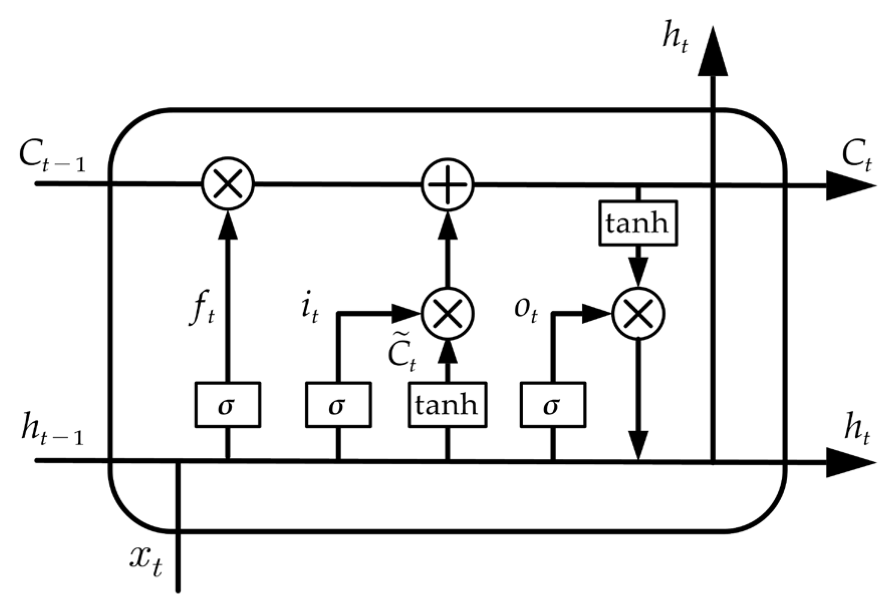
In contrast to traditional Recurrent Neural Networks (RNNs), Long Short-Term Memory (LSTM) overcomes the vanishing and exploding gradient issues when processing long sequential data. By embedding a gating mechanism, the model selectively retains and updates certain information, thereby effectively capturing long-term dependencies in a time series [55].
Specifically, the LSTM model achieves its functionality through three types of gating structures: the forget gate, the input gate, and the output gate. Figure 2 illustrates the structure of the cell in this model.
(1) The forget gate. The forget gate selectively discards certain information from the previous cell state, thereby mitigating the gradient-related instability and facilitating the integration of new information. The calculation formula is as follows:
f t = σ ( W f · h t 1 , x t + b f )
where f t denotes the proportion of information retained at time step t, W f is the weight matrix, b f is the bias term, h t 1 represents the hidden state of the previous time step, and x t represents the input of the current time step. When predicting construction industry carbon emissions, the forget gate enables the model to progressively shed historical high-emission growth patterns while adapting to data variations driven by the low-carbon policy implementation.
(2) The input gate. The input gate regulates the proportion of new information written into the candidate state C ~ t via the gating vector i t , which can be formulated as follows:
i t = σ W i · h t 1 , x t + b i C ~ t = tanh W c · h t 1 , x t + b C C t = f t · C t 1 + i t · C ~ t
where C t denotes the updated cell state. The dynamic update mechanism of the input gate determines the extent to which current time step carbon emission data is integrated into the model, thereby enabling continuous memory refinement and the effective prediction of evolving data trajectories.
(3) The output gate. This gate structure controls the exposure level of information contained in the cell state C t through the gating vector o t , thereby generating the hidden state h t for the current time step. Its formula is defined as follows:
o t = σ W o · h t 1 , x t + b o h t = o t · tanh ( C t )
Notably, h t can serve as both the output of the current time step and as a component of the cell state for the next time step, thereby participating in subsequent gating computations. The output gate ensures that only the long-term memory features critical for current predictions are integrated into the hidden state h t while suppressing noise interference unrelated to short-term fluctuations. With this structure, the model’s capacity for characterizing nonlinear time series patterns is significantly enhanced.
Given the time-lag effects of macro-control policies on the construction industry, this study employs the LSTM model to conduct time series forecasting for construction carbon emissions [56].

2.3. Evaluation Metrics

To comprehensively evaluate the predictive performance of different models, the following metrics are utilized in this study:
(1) Mean Squared Error (MSE). MSE is used to quantify the average squared difference between the predicted values and the actual values, which emphasizes larger discrepancies. The formula for MSE is as follows:
M S E = 1 N t = 1 N ( x t x ^ t ) 2
where x t denotes the actual value at period t and x ^ t denotes the predicted value.
(2) Mean Absolute Error (MAE). MAE measures the average absolute deviation between the predicted and actual values, offering a straightforward assessment of the predictive performance. The formula for MAE is as follows:
M A E = 1 N t = 1 N x t x ^ t
(3) Root Mean Squared Relative Error (RMSRE). RMSRE quantifies the average extent of relative discrepancies between the actual values and the forecast results. By squaring the relative errors prior to averaging, this metric heightens its sensitivity to outliers and allows for the evaluation of data with varying magnitudes.
R M S R E = 1 N t = 1 N x t x ^ t x t 2
(4) Mean Absolute Percentage Error (MAPE). MAPE assesses the average level of prediction errors in percentage terms. Compared to RMSRE, this metric is also dimensionless but places greater emphasis on reflecting the overall deviation of the prediction results, which enables a more robust evaluation.
M A P E = 1 N t = 1 N x t x ^ t x t
The selection of these evaluation metrics enables a thorough assessment of both the extreme deviations and the overall accuracy of the prediction results, which in turn facilitates the derivation of more objective and solid experimental conclusions.

3. Case Study

3.1. In-Sample Forecasting Results and Analysis

3.1.1. SVR-Based Predictions

The STIRPAT model offers an effective approach to examine the joint impacts of population-related, economic, and technological factors on the environment through regression analysis. Therefore, the model is employed in this study as an analytical framework to investigate the nonlinear relationships between carbon emissions and influential factors. To thoroughly assess both linear and nonlinear correlations between potential drivers and carbon emissions, a dual-method approach combining Pearson correlation analysis and grey relational analysis is employed. From an initial pool of 20 candidate factors, five significant determinants are identified: construction workforce (in million people), urban resident population (in million people), urbanization rate, total energy consumption of the construction industry (TECCI, in million tons of standard coal equivalent), and construction output per capita (COPC, in kCNY/capita). Notably, the COPC is calculated as the ratio of the total construction output value to the workforce size. The dataset includes the carbon emissions from the construction industry and associated influential factors from 1997 to 2021. The emission data are sourced from the sector-specific inventory in the China Emission Accounts and Datasets (CEADs) [4,5,6,7], while the data for the factors are derived from the China Statistical Yearbook [57]. Descriptive statistics of the variables are presented in Table 1.
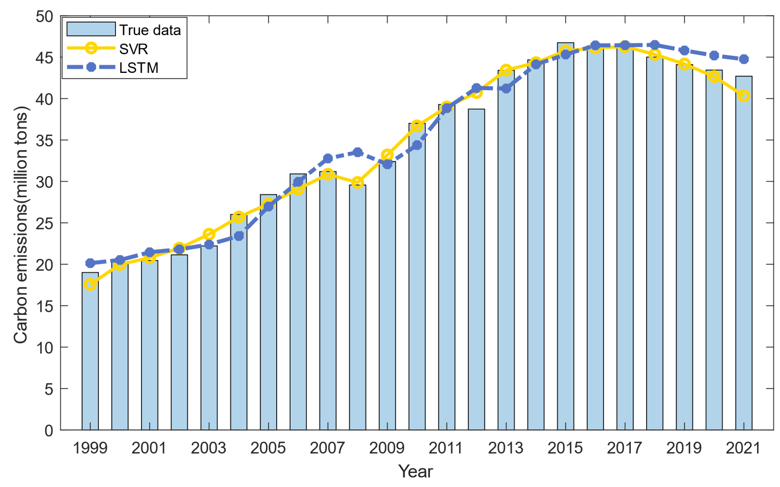
The SVR model is constructed based on the carbon emissions data and associated influential factors from 1997 to 2018 and subsequently validated using the test dataset for the period 2019–2021. The prediction result is shown in Figure 3. As depicted in Figure 3, the SVR model exhibits remarkable consistency across the different datasets, achieving a training accuracy of 97.61% and a test accuracy of 97.50%. These metrics substantiate the proficiency of the model in quantifying the nonlinear relationships between carbon emissions and influential factors, while its ε -insensitive loss function ensures resilience to outlier interference. Therefore, the SVR model is highly applicable for predicting the carbon emissions in the construction industry, which provides a reliable foundation for both academic research and the development of practical mitigation strategies.

3.1.2. LSTM-Based Predictions

The windowing method is utilized in this study to develop an LSTM model tailored for time series prediction. Specifically, at each time step, the model processes two years of sequential data to predict the carbon emissions for the next year, thereby enabling continuous integration of the emerging trajectories. Figure 3 illustrates that the predicted trend from the LSTM model closely matches with the historical data, which is evidenced by its training accuracy of 95.94% and test accuracy of 95.75%. This finding underscores the model’s remarkable adaptability and confirms its capacity to deliver accurate and robust carbon emission projections for the construction industry.
While both the SVR and LSTM models demonstrate high forecast accuracy, their predictive performance varies considerably across different phases. Figure 4 illustrates the forecast errors of the SVR and LSTM models. As evidenced in Figure 4, the SVR model shows pronounced error fluctuations during the initial and terminal phases of the time series (1999–2006 and 2014–2021), whereas the LSTM model displays a weakened sensitivity to mid-term (2007–2013) data variability. This suggests that the SVR model achieves superior performance in mid-term predictions, while the LSTM model remains uniquely effective in extracting the critical temporal features at both boundaries of the sequence.
Furthermore, the residuals of the two models exhibit opposite signs relative to the zero-error baseline during specific periods (e.g., 2007 and 2021, in Figure 4). Such error symmetry implies that integrating individual models into a combination forecasting model can drive residuals closer to the theoretical optimum, thereby effectively reducing prediction uncertainty. These findings provide a methodological framework for enhancing the accuracy and robustness of carbon emission prediction through forecast combination techniques.

3.1.3. GIOWA Combination Forecasting Results

The GIOWA combination forecasting model is developed based on the existing individual prediction models SVR and LSTM. To contrast with the previous sub-models and highlight the effects of different averaging exponents, five specific values of the λ (λ = 1, λ → 0, λ = −1, λ = 1/2, and λ = 1/4) are empirically determined, with prediction accuracy employed as the induced variable α i t   ( i = 1,2 ;   t = 1,2 , , 23 ) . Subsequently, by solving the quadratic programming models under the minimum SSE criterion, optimal weight combinations are derived, which enables the generation of the GIOWA combination forecasting results. The key calculation process is presented below.
(1) When λ = 1, the GIOWA model reduces to the conventional IOWA combination forecasting model, with its λ-th power error information matrix expressed as follows:
R 1 = 14.7209 5.9096 5.9096 71.3109
Under the principle of SSE minimization, the corresponding optimization model is formulated as follows:
min S 1 = 14.7209 w 1 2 + 71.3109 w 2 2 + 11.8192 w 1 w 2   s . t . w 1 + w 2 = 1 w 1 , w 2 0
and the optimal weights are w 1 = 0.8810 and w 2 = 0.1190 . Thus, the corresponding IOWA model is x ^ t = 0.8810 x α i n d e x 1 t + 0.1190 x α i n d e x 2 t .
(2) When λ → 0, the model converges to the IOWGA model, with its λ-th power error information matrix expressed as follows:
R 0 = 0.0136 0.0050 0.0050 0.0710
Driven by the objective of minimizing the SSE, the quadratic programming model is established as follows:
min S 0 = 0.0136 w 1 2 + 0.0710 w 2 2 + 0.0100 w 1 w 2 s . t . w 1 + w 2 = 1 w 1 , w 2 0
The corresponding optimal weights are w 1 = 0.8840 and w 2 = 0.1160 . Therefore, the IOWGA model is given by x ^ t = 0.8840 x α i n d e x 1 t 0.1160 x α i n d e x 2 t .
(3) When λ = −1, the original model transforms into the IOWHA model, with its λ-th power error information matrix expressed as follows:
R 1 = 1.88 × 10 5 6.06 × 10 7 6.06 × 10 7 9.23 × 10 5
Thus, the corresponding optimization model is formulated as follows:
min S 1 = 1.88 × 10 5 w 1 2 + 9.23 × 10 5 w 2 2 + 1.21 × 10 6 w 1 w 2 s . t . w 1 + w 2 = 1 w 1 , w 2 0
Given the optimal weights w 1 = 0.8340 and w 2 = 0.1660 , the IOWHA model can be presented as x ^ t = ( 0.8340 x α i n d e x ( 1 t ) + 0.1660 x α i n d e x ( 2 t ) ) 1 .
(4) When λ = 1/2, the λ-th power error information matrix of the GIOWA model is as follows:
R 1 / 2 = 0.1066 0.0446 0.0446 0.5451
Subsequently, the corresponding optimization model is as follows:
min S 1 / 2 = 0.1066 w 1 2 + 0.5451 w 2 2 + 0.0891 w 1 w 2 s . t . w 1 + w 2 = 1 w 1 , w 2 0
Therefore, the optimal weights are w 1 = 0.8900 and w 2 = 0.1100 , and the expression of the GIOWA model is x ^ t = ( 0.8900 x α i n d e x 1 t 1 / 2 + 0.1100 x α i n d e x 2 t 1 / 2 ) 2 .
(5) When λ = 1/4, the λ-th power error information matrix of the GIOWA model is as follows:
R 1 / 4 = 0.0047 0.0019 0.0019 0.0244
Therefore, its quadratic programming model is presented as follows:
min S 1 / 4 = 0.0047 w 1 2 + 0.0244 w 2 2 + 0.0038 w 1 w 2 s . t . w 1 + w 2 = 1 w 1 , w 2 0
Since the optimal weights are w 1 = 0.8900 and w 2 = 0.1100 , the expression of the GIOWA model is x ^ t = ( 0.8890 x α i n d e x 1 t 1 / 4 + 0.1110 x α i n d e x 2 t 1 / 4 ) 4 .
Figure 5 shows the comparative forecasting errors between the individual models and certain GIOWA models during the sample period. The prediction results indicate that the GIOWA combination forecasting models with varying λ significantly outperform LSTM and SVR, exhibiting a lower overall deviation and a more stable error fluctuation. This improvement demonstrates the effectiveness of the GIOWA model in reducing systematic biases and random errors, highly attributable to its dynamic weighting mechanism and SSE minimization criterion.
Notably, in 2012, all the combination forecasting models failed to improve the prediction accuracy of the individual models. The direct cause is that both the SVR and LSTM models demonstrated negative deviations relative to the actual value, indicating that the inclusion of another individual model did not provide additional effective information for the GIOWA model. Furthermore, this phenomenon is attributed to prior policy interventions that intensified systemic uncertainties and thereby complicated the short-term trend forecasting. Specifically, following the 2009 Copenhagen Climate Change Conference, China issued the Notice on Carrying Out Pilot Work for Low-Carbon Provinces and Cities in 2010 [58]. This notice introduced supporting policies aimed at establishing a low-carbon industrial system and data management framework. These policy adjustments intensified the instability of the socio-economic system transformation, leading to sudden and nonlinear fluctuations in carbon emissions during the policy implementation periods.
To thoroughly assess the forecast performance of the GIOWA model, four key error metrics are selected to evaluate both the extreme deviations and the overall accuracy of the prediction results, including MSE, MAE, RMSRE, and MAPE. The error comparison between the individual models and the GIOWA models is presented in Table 2, while Table 3 provides a detailed comparison between the GIOWA models and other combination models.
From Table 2, it can be seen that the five GIOWA models consistently outperform the individual models across all error metrics, and as evidenced in Table 3, they also demonstrate enhanced predictive accuracy compared to other combination forecasting models. This confirms the superiority of the GIOWA model in modeling the evolving trajectories of construction carbon emissions. Additionally, the models superior for the MSE or RMSRE tend to minimize extreme deviations, whereas models with better predictive performance for the MAE or MAPE demonstrate enhanced robustness against data fluctuations. Therefore, λ = 1/4 is identified as the optimal averaging exponent among the current set of values, which effectively balances precision and stability in practical carbon emissions forecasting.

3.2. Out-of-Sample Forecasting Results and Analysis

3.2.1. Prediction Results of Individual Models

To provide evidence-based decision support for policy formulation, this study further investigates the evolving trajectories of construction carbon emissions from 2022 to 2030. The SVR and LSTM models are initially utilized for individual forecasts. Subsequently, the GIOWA model is developed using the averaging exponent λ = 1/4.
Since SVR forecasting for the out-of-sample period requires the prior estimation of five influential factors, and these factors all show certain linear growth trends, double exponential smoothing (DES) models are established for numerical projections. The prediction errors and accuracy of each influential factor by DES are shown in Table 4.
As shown in Figure 3, although the LSTM predictions have reflected the downward trend of the observed data since 2017, the predicted values are higher than the actual values. This divergence indicates that if the prediction values of the LSTM model are directly integrated into rolling forecasts, it may result in a trend discontinuity at the junction between the sample period and the forecast period. To mitigate this issue, the GM (1, 1) model is first utilized to simulate the decline in carbon emissions from 2017 to 2021. The model achieves remarkable fitting accuracy (R2 > 95%), confirming its effectiveness in handling short-term time series [59]. Subsequently, the input dataset of the LSTM model is reconstructed based on projections derived from the GM (1, 1), which significantly refines the predictive sequence continuity of the LSTM model and results in optimized forecast smoothness.

3.2.2. Prediction Results of the GIOWA Model

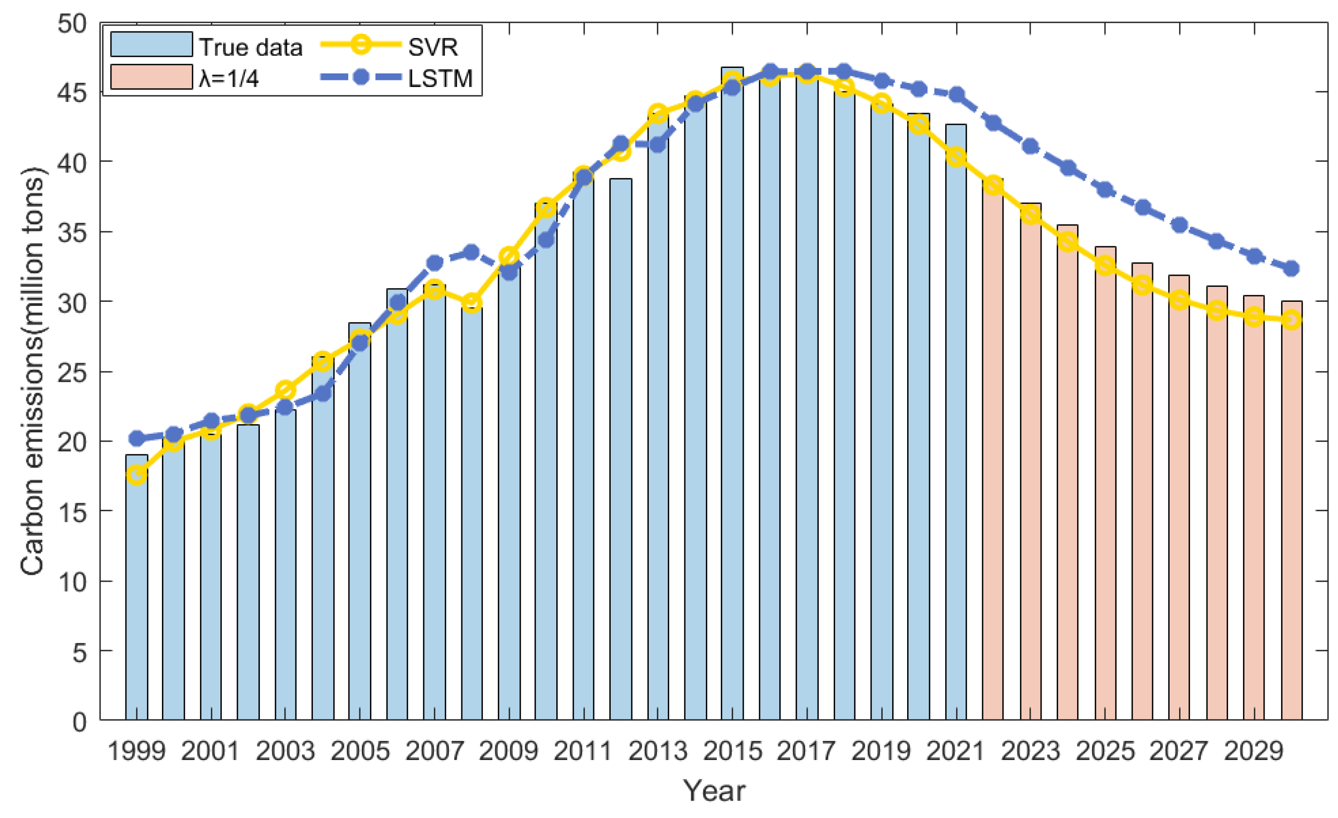
The GIOWA model dynamically assigns descending weights to individual models in each period according to their prediction performance. However, the actual carbon emissions during the forecast period remain unknown, hindering the calculation of individual model accuracies. Therefore, this study first estimates the construction industry carbon emissions for 2022–2030 using the historical average weights of the individual models. Specifically, the estimation formula is expressed as x t = 0.5846 x 1 t + 0.4154 x 2 t , where x 1 t and x 2 t denote the prediction values from the SVR and LSTM models, respectively. Subsequently, the rolling forecast method is adopted to continuously incorporate the new information corresponding to external changes into the decision-making scope, thereby responding adaptively to the changing forecasting conditions. Table 5 illustrates the optimal combination weights and GIOWA prediction outcomes for each year during the rolling forecasting process. Figure 6 illustrates the forecast results of both the individual models and the GIOWA model from 1999 to 2030.
As depicted in Figure 6, the prediction results of the GIOWA combination forecasting model demonstrate that the carbon emissions in China’s construction industry will continue to decrease throughout the 2022–2030 period. This trend highly aligns with the development principle outlined in the 14th Five-Year Plan of China, which emphasizes promoting energy conservation in key carbon-emitting sectors including the construction industry [60]. Additionally, it is projected that the construction carbon emissions in China will reduce to 29.99 million tons of CO2 by 2030, which represents a reduction of nearly 35% compared to the peak of 46.52 million tons in 2017. As a leading advocate for the Paris Agreement, China is leveraging its breakthroughs in renewable energy and low-carbon technologies to enhance energy efficiency and reduce carbon emissions, thereby advancing the establishment of a fair and cooperative global climate governance framework. Notably, a deceleration in the carbon emission reduction rate from 4.81% to 1.66% is projected during the forecast period. This underscores the imperative for the Chinese government to expand the scope of existing carbon emission governance and to foster cross-sectoral collaborative efforts, thus ensuring the timely realization of the dual carbon goals.

4. Conclusions

The increasingly severe challenges posed by climate change necessitate precise prediction and monitoring, and timely mitigation measures for carbon emissions. To accurately assess the carbon emission reduction potential of China’s construction industry and provide evidence-based decision support for policy formulation, this study develops a GIOWA combination forecasting model based on historical data from 1997 to 2021. Further projections are made for the period 2022–2030. In summary, the research yields the following conclusions:
(1)
Both SVR and LSTM models prove to be effective for forecasting carbon emissions in China’s construction industry, with their accuracy surpassing 95%. The prediction results of the SVR and LSTM models indicate that the carbon emissions in China’s construction industry will continue to decrease from 2022 to 2030. Therefore, the Chinese government should implement targeted strategies, including moderating the labor demands of the construction industry [61], advancing new-type urbanization [62], and optimizing the energy consumption structure [63,64], so as to sustain the downward trend in construction carbon emissions. Given that the residuals of the SVR and LSTM models exhibit opposite signs relative to the zero-error baseline, the prediction accuracy can be further enhanced with forecast combination techniques.
(2)
The GIOWA combination forecasting model demonstrates superior predictive performance across varying averaging exponent λ, with all prediction accuracy exceeding 98%, outperforming the individual models on four key error metrics including RMSRE and MAPE. Therefore, the GIOWA model is more effective and accurate in capturing nonlinear variation characteristics in construction carbon emissions and generating reliable projections. Based on the forecast results, the carbon emissions of the construction industry will reduce to 29.99 million tons of CO2 by 2030, representing a reduction of nearly 35% compared to the peak of 46.52 million tons in 2017. This indicates that the construction industry in China is transitioning from extensive development patterns to green intensive practices, attributable to China’s nationwide promotion of prefabricated buildings [65] and energy-efficient construction technologies [66,67]. However, given that a deceleration in the carbon emission reduction rate from 4.81% to 1.66% is projected during the forecast period, the Chinese government, the construction industry, and relevant sectors must collaborate closely to guarantee the timely realization of the dual carbon goals.
(3)
There are certain limitations in this study. Current analysis is established on national-level annual emission data due to availability constraints. Subsequent studies can employ provincial or municipal datasets with a quarterly or monthly frequency to enhance spatial resolution and temporal granularity, thereby facilitating real-time emission monitoring and the implementation of dynamic early-warning mechanisms. Additionally, the current research remains deficient in exploring the impact of uncertainty on the combination forecasting results. This gap will be addressed and investigated more thoroughly in future studies.

Author Contributions

Conceptualization, T.H. and Z.B.; methodology, T.H., Z.B. and B.Z.; software, T.H.; validation, T.H., Z.B. and B.Z.; formal analysis, T.H.; resources, X.G.; data curation, T.H. and X.G.; writing—original draft preparation, T.H. and Z.B.; writing—review and editing, T.H., B.Z. and X.G.; visualization, T.H.; supervision, X.G.; project administration, X.G.; funding acquisition, X.G. All authors have read and agreed to the published version of the manuscript.

Funding

This research was funded by Provincial College Student Innovation and Entrepreneurship Training Program grant number 202410307246Y.

Data Availability Statement

The data for the carbon emissions of the construction industry can be found at https://www.ceads.net.cn/data/nation/ (accessed on 20 November 2024). The data for all influential factors can be found at https://data.cnki.net/yearBook/single?id=N2024110295 (accessed on 20 November 2024). The specific data used in this study has been organized and uploaded to a GitHub repository. The URL is: https://github.com/speechxalter/Original-data (accessed on 29 May 2025).

Conflicts of Interest

The authors declare no conflicts of interest.

Abbreviations

The following abbreviations are used in this manuscript:
GIOWAGeneralized induced ordered weighted averaging
SVRSupport vector regression
LSTMLong short-term memory
GMGrey model
OWAOrdered weighted averaging
IOWAInduced ordered weighted averaging
IOWGAInduced ordered weighted geometric averaging
IOWHAInduced ordered weighted harmonic averaging
SSESum of squared errors
TECCITotal energy consumption of the construction industry
COPCConstruction output per capita
SASimple averaging
IVWInverse Variance Weighting
BMABayesian Model Averaging
BGOCBates Granger optimal combination
MSEMean squared error
MAEMean absolute error
RMSRERoot mean squared relative error
MAPEMean absolute percentage error

References

  1. U.S. Congress. S. 4355—Clean Competition Act. Available online: https://www.congress.gov/bill/117th-congress/senate-bill/4355 (accessed on 13 September 2024).
  2. European Parliament and Council of the European Union. Regulation (EU) 2023/956 Establishing a Carbon Border Adjustment Mechanism. Available online: http://data.europa.eu/eli/reg/2023/956/oj (accessed on 17 September 2024).
  3. State Council of the People’s Republic of China. Opinions on Fully, Accurately, and Comprehensively Implementing New Development Concepts to Achieve Carbon Peaking and Carbon Neutrality. Available online: https://www.gov.cn/zhengce/2021-10/24/content_5644613.htm (accessed on 7 September 2024).
  4. Guan, Y.; Shan, Y.; Huang, Q.; Chen, H.; Wang, D.; Hubacek, K. Assessment to China’s Recent Emission Pattern Shifts. Earths Future 2021, 9, e2021EF002241. [Google Scholar] [CrossRef]
  5. Shan, Y.; Guan, D.; Zheng, H.; Ou, J.; Li, Y.; Meng, J.; Mi, Z.; Liu, Z.; Zhang, Q. China CO2 emission accounts 1997–2015. Sci. Data 2018, 5, 170201. [Google Scholar] [CrossRef] [PubMed]
  6. Shan, Y.; Huang, Q.; Guan, D.; Hubacek, K. China CO2 emission accounts 2016–2017. Sci. Data 2020, 7, 54. [Google Scholar] [CrossRef] [PubMed]
  7. Xu, J.; Guan, Y.; Oldfield, J.; Guan, D.; Shan, Y. China carbon emission accounts 2020–2021. Appl. Energy 2024, 360, 122837. [Google Scholar] [CrossRef]
  8. Wang, H.; Wei, Z.; Fang, T.; Xie, Q.; Li, R.; Fang, D. Carbon Emissions Prediction Based on the GIOWA Combination Forecasting Model: A Case Study of China. J. Clean. Prod. 2024, 445, 141340. [Google Scholar] [CrossRef]
  9. Ehrlich, P.R.; Holdren, J.P. Impact of Population Growth. Science 1971, 171, 1212–1217. [Google Scholar] [CrossRef]
  10. González-Torres, M.; Pérez-Lombard, L.; Coronel, J.; Maestre, I. Revisiting Kaya Identity to define an Emissions Indicators Pyramid. J. Clean. Prod. 2021, 317, 128328. [Google Scholar] [CrossRef]
  11. Dietz, T.; Rosa, E.A. Effects of Population and Affluence on CO2 Emissions. Proc. Natl. Acad. Sci. USA 1997, 94, 175–179. [Google Scholar] [CrossRef]
  12. Zhou, X.; Hu, P.; Cheng, P. Carbon Emission Accounting and Carbon Peak Prediction of China’s Construction Industry from a Life-Cycle Perspective. Chin. J. Environ. Sci. 2025, 46, 2020–2034. [Google Scholar]
  13. Zhang, S.; Huo, Z.; Zhai, C. Building Carbon Emission Scenario Prediction Using STIRPAT and GA-BP Neural Network Model. Sustainability 2022, 14, 9369. [Google Scholar] [CrossRef]
  14. Li, L.; Li, Y. The Spatial Relationship between CO2 Emissions and Economic Growth in the Construction Industry: Based on the Tapio Decoupling Model and STIRPAT Model. Sustainability 2023, 15, 528. [Google Scholar] [CrossRef]
  15. Kang, X.; Chen, L.; Wang, Y.; Liu, W. Analysis on the Spatial Correlation Network and Driving Factors of Carbon Emissions in China’s Logistics Industry. J. Environ. Manag. 2024, 366, 121916. [Google Scholar] [CrossRef] [PubMed]
  16. Bai, D.; Dong, Q.; Khan, S.A.R.; Li, J.; Wang, D.; Chen, Y.; Wu, J. Spatio-Temporal Heterogeneity of Logistics CO2 Emissions and Their Influencing Factors in China: An Analysis Based on Spatial Error Model and Geographically and Temporally Weighted Regression Model. Environ. Technol. Innov. 2022, 28, 102791. [Google Scholar] [CrossRef]
  17. Chen, L.; Pan, Y.; Zhang, D. Prediction of Carbon Emissions Level in China’s Logistics Industry Based on the PSO-SVR Model. Mathematics 2024, 12, 1980. [Google Scholar] [CrossRef]
  18. Wen, L.; Song, Q. The Forecasting Model Research of Rural Energy Transformation in Henan Province Based on STIRPAT Model. Environ. Sci. Pollut. Res. 2022, 29, 75550–75565. [Google Scholar] [CrossRef]
  19. Chen, J.; Jia, J.; Wang, L.; Zhong, C.; Wu, B. Carbon Reduction Countermeasure from a System Perspective for the Electricity Sector of Yangtze River Delta (China) by an Extended Logarithmic Mean Divisia Index (LMDI). Systems 2023, 11, 117. [Google Scholar] [CrossRef]
  20. Rao, C.; Zhang, Y.; Wen, J.; Xiao, X.; Goh, M. Energy Demand Forecasting in China: A Support Vector Regression-Compositional Data Second Exponential Smoothing Model. Energy 2023, 263, 125955. [Google Scholar] [CrossRef]
  21. Alhindawi, R.; Abu Nahleh, Y.; Kumar, A.; Shiwakoti, N. Projection of Greenhouse Gas Emissions for the Road Transport Sector Based on Multivariate Regression and the Double Exponential Smoothing Model. Sustainability 2020, 12, 9152. [Google Scholar] [CrossRef]
  22. Gao, M.; Yang, H.; Xiao, Q.; Goh, M. A Novel Method for Carbon Emission Forecasting Based on Gompertz’s Law and Fractional Grey Model: Evidence from American Industrial Sector. Renew. Energy 2022, 181, 803–819. [Google Scholar] [CrossRef]
  23. Zhang, R.; Mao, S.; Kang, Y. A Novel Traffic Flow Prediction Model: Variable Order Fractional Grey Model Based on an Improved Grey Evolution Algorithm. Exp. Syst. Appl. 2023, 224, 119943. [Google Scholar] [CrossRef]
  24. Zhang, S.; Wu, L.; Cheng, M.; Zhang, D. Prediction of Whole Social Electricity Consumption in Jiangsu Province Based on Metabolic FGM (1, 1) Model. Mathematics 2022, 10, 1791. [Google Scholar] [CrossRef]
  25. Sirisha, U.M.; Belavagi, M.C.; Attigeri, G. Profit Prediction Using ARIMA, SARIMA and LSTM Models in Time Series Forecasting: A Comparison. IEEE Access 2022, 10, 124715–124727. [Google Scholar] [CrossRef]
  26. Ning, L.; Pei, L.; Li, F. Forecast of China’s Carbon Emissions Based on ARIMA Method. Discret. Dyn. Nat. Soc. 2021, 2021, 1441942. [Google Scholar] [CrossRef]
  27. Zhong, W.; Zhai, D.; Xu, W.; Gong, W.; Yan, C.; Zhang, Y.; Qi, L. Accurate and Efficient Daily Carbon Emission Forecasting Based on Improved ARIMA. Appl. Energy 2024, 376, 124232. [Google Scholar] [CrossRef]
  28. Jiang, H.; Yin, J.; Wei, D.; Luo, X.; Ding, Y.; Xia, R. Industrial Carbon Emission Efficiency Prediction and Carbon Emission Reduction Strategies Based on Multi-Objective Particle Swarm Optimization-Backpropagation: A Perspective from Regional Clustering. Sci. Total Environ. 2024, 906, 167692. [Google Scholar] [CrossRef]
  29. Sun, W.; Huang, C. Predictions of Carbon Emission Intensity Based on Factor Analysis and an Improved Extreme Learning Machine from the Perspective of Carbon Emission Efficiency. J. Clean. Prod. 2022, 338, 130414. [Google Scholar] [CrossRef]
  30. Lv, Q.; Rashidi-Khaniabadi, A.; Zheng, R.; Zhou, T.; Mohammadi, M.-R.; Hemmati-Sarapardeh, A. Modelling CO2 diffusion coefficient in heavy crude oils and bitumen using extreme gradient boosting and Gaussian process regression. Energy 2023, 275, 127396. [Google Scholar] [CrossRef]
  31. Liu, M.; Qi, L.; Chen, H.; Luo, X.; Zhu, X.; Chen, C. Study on the Spatialization of Anthropogenic Carbon Emissions in China Based on SVR-ZSSR. Sci. Rep. 2023, 13, 1887. [Google Scholar] [CrossRef]
  32. Ahmed, A.A.; Badri, Y.; Shamseldin, A. Application of Nonlinear Gaussian Process Regression Models for CO2 Emissions Prediction. In Proceedings of the International Conference on Innovations in Information Technology, Al Ain, United Arab Emirates, 14–15 November 2023. [Google Scholar]
  33. Chen, H.; Wang, B.; Huang, Z. Greenhouse Gas Emission Prediction and Impact Analysis of Dual-Fuel Engine. Process. Saf. Environ. 2024, 191, 1–13. [Google Scholar] [CrossRef]
  34. Kumari, S.; Singh, S.K. Machine Learning-Based Time Series Models for Effective CO2 Emission Prediction in India. Environ. Sci. Pollut. Res. 2023, 30, 116601–116616. [Google Scholar] [CrossRef]
  35. Larsson, G.; Maire, M.; Shakhnarovich, G. FractalNet: Ultra-Deep Neural Networks without Residuals. arXiv 2016, arXiv:1605.07648. [Google Scholar]
  36. Shakhovska, N.; Shymanskyi, V.; Prymachenko, M. FractalNet-LSTM Model for Time Series Forecasting. Comput. Mater. Contin. 2025, 82, 4469–4484. [Google Scholar] [CrossRef]
  37. Li, Y. Forecasting Chinese Carbon Emissions Based on a Novel Time Series Prediction Method. Energy Sci. Eng. 2020, 8, 2274–2285. [Google Scholar] [CrossRef]
  38. Lichtendahl, K.C.; Winkler, R.L. Why do some combinations perform better than others? Int. J. Forecast. 2020, 36, 142–149. [Google Scholar] [CrossRef]
  39. Diebold, F.X.; Shin, M. Machine learning for regularized survey forecast combination: Partially-egalitarian LASSO and its derivatives. Int. J. Forecast. 2019, 35, 1679–1691. [Google Scholar] [CrossRef]
  40. Alexander, N.; Scherer, W.; Burkett, M. Extending the Markowitz model with dimensionality reduction: Forecasting efficient frontiers. In Proceedings of the 2021 Systems and Information Engineering Design Symposium, Charlottesville, VA, USA, 29–30 April 2021. [Google Scholar]
  41. Ortiz, R.; Contreras, M.; Mellado, C. Regression, Multicollinearity and Markowitz. Financ. Res. Lett. 2023, 58, 104550. [Google Scholar] [CrossRef]
  42. Botero, S.; García Mazo, C.M.; Moreno Arboleda, F.J. Power generation mix in Colombia including wind power: Markowitz portfolio efficient frontier analysis with machine learning. J. Open Innov. Technol. Mark. Complex. 2024, 10, 100402. [Google Scholar] [CrossRef]
  43. Nowotarski, J.; Raviv, E.; Trück, S.; Weron, R. An empirical comparison of alternative schemes for combining electricity spot price forecasts. Energy Econ. 2014, 46, 395–412. [Google Scholar] [CrossRef]
  44. Lv, X.; Yin, K.; Li, X. Grey Multivariate Variable Weight Combination Prediction Model and Its Application. Stat. Decis. 2022, 38, 25–29. [Google Scholar]
  45. Yager, R.R. On Ordered Weighted Averaging Aggregation Operators in Multicriteria Decision Making. IEEE Trans. Syst. Man Cybern. 1988, 18, 183–190. [Google Scholar] [CrossRef]
  46. Lu, P.; Yang, J.; Ye, L.; Zhang, N.; Wang, Y.; Di, J.; Gao, Z.; Wang, C.; Liu, M. A novel adaptively combined model based on induced ordered weighted averaging for wind power forecasting. Renew. Energy 2024, 226, 120350. [Google Scholar] [CrossRef]
  47. Yang, H.; Wang, M.; Li, G. A combined prediction model based on secondary decomposition and intelligence optimization for carbon emission. Appl. Math. Model 2023, 121, 484–505. [Google Scholar] [CrossRef]
  48. Cheng, X.; Chen, W. Research on Air Logistics Demand Forecasting Based on Induced Ordered Weighted Geometric Averaging Operator. J. Civ. Aviat. 2024, 8, 6–10+59. [Google Scholar]
  49. Li, S.; Wang, Q.; Jiang, X.; Li, R. The Negative Impact of the COVID-19 on Renewable Energy Growth in Developing Countries: Underestimated. J. Clean. Prod. 2022, 367, 132996. [Google Scholar] [CrossRef]
  50. Wang, Q.; Li, S.; Li, R. Will Trump’s coal revival plan work?—Comparison of results based on the optimal combined forecasting technique and an extended IPAT forecasting technique. Energy 2019, 169, 762–775. [Google Scholar] [CrossRef]
  51. Qiu, H.; Yang, Y.; Li, D. Research on Subgrade Settlement Prediction Based on Equidistance Processing and IOWHA Operator. Sci. Technol. Eng. 2022, 22, 8884–8892. [Google Scholar]
  52. Song, X.; Liang, G.; Li, C.; Chen, W. Electricity Consumption Prediction for Xinjiang Electric Energy Replacement. Math. Probl. Eng. 2019, 2019, 3262591. [Google Scholar] [CrossRef]
  53. Zhou, H.; Qi, F.; Liu, C.; Liu, G.; Xiao, G. Predicting combined carbon emissions in urban regions considering micro-level enterprise electricity consumption data and macro-level regional data. Front. Energy Res. 2024, 12, 1343318. [Google Scholar] [CrossRef]
  54. Du, Z.; Liu, Y.; Zhang, Z. Spatiotemporal Analysis of Influencing Factors of Carbon Emission in Public Buildings in China. Buildings 2022, 12, 424. [Google Scholar] [CrossRef]
  55. Lindemann, B.; Müller, T.; Vietz, H.; Jazdi, N.; Weyrich, M. A Survey on Long Short-Term Memory Networks for Time Series Prediction. In Proceedings of the 14th CIRP Conference on Intelligent Computation in Manufacturing Engineering, Naples, Italy, 15–17 July 2020. [Google Scholar]
  56. Millar, J.N.; Oliner, S.D.; Sichel, D.E. Time-To-Plan Lags for Commercial Construction Projects. Reg. Sci. Urban Econ. 2016, 59, 75–89. [Google Scholar] [CrossRef]
  57. National Bureau of Statistics of China. China Statistical Yearbook 2024; China Statistics Press: Beijing, China, 2024. Available online: https://www.stats.gov.cn/sj/ndsj/2024/indexeh.htm (accessed on 20 November 2024).
  58. National Development and Reform Commission. Notice on Carrying out Pilot Work for Low-Carbon Provinces and Cities. Available online: https://www.ndrc.gov.cn/xxgk/zcfb/tz/201008/t20100810_964674.html (accessed on 21 January 2025).
  59. Lei, Y.; Guo, M.; Zhao, D.; Cai, H.; Hu, D. Application of Grey Model GM(1, 1) to Ultra Short-Term Predictions of Universal Time. Artif. Satell. 2016, 51, 19–29. [Google Scholar] [CrossRef]
  60. State Council of the People’s Republic of China. The 14th Five-Year Plan for National Economic and Social Development of the People’s Republic of China and the Long-Range Objectives Through the Year 2035. Available online: https://www.gov.cn/xinwen/2021-03/13/content_5592681.htm (accessed on 7 February 2025).
  61. Ye, S. The Impact of Low-Carbon City Pilot Policy on Corporate Labor Demand: Demand Scale, Structural Adjustment and Mechanisms. J. Tech. Econ. Manag. 2024, 9, 87–92. [Google Scholar]
  62. Chen, W.; Wang, G.; Xu, N.; Ji, M.; Zeng, J. Promoting or Inhibiting? New-Type Urbanization and Urban Carbon Emissions Efficiency in China. Cities 2023, 140, 104429. [Google Scholar] [CrossRef]
  63. Zhang, J.; Liu, Y.; Saqib, N.; Waqas Kamran, H. An Empirical Study on the Impact of Energy Poverty on Carbon Intensity of the Construction Industry: Moderating Role of Technological Innovation. Front. Environ. Sci. 2022, 10, 929939. [Google Scholar] [CrossRef]
  64. Jiang, T.; Li, S.; Yu, Y.; Peng, Y. Energy-Related Carbon Emissions and Structural Emissions Reduction of China’s Construction Industry: The Perspective of Input–Output Analysis. Environ. Sci. Pollut. Res. 2022, 29, 39515–39527. [Google Scholar] [CrossRef]
  65. Wang, X.; Xie, S.; Wei, Z.; Wang, J. A Study on the Impact of China’s Prefabricated Building Policy on the Carbon Reduction Benefits of China’s Construction Industry Based on a Difference-in-Differences Method. Sustainability 2024, 16, 7606. [Google Scholar] [CrossRef]
  66. Lu, H.; Juan, Y.-K. Optimal Decision-Making Model for Selecting Residential Green Building Technologies in China. Front. Environ. Sci. 2022, 10, 973334. [Google Scholar] [CrossRef]
  67. Wu, H.; Deng, F.; Tan, H. Research on Parametric Design Method of Solar Photovoltaic Utilization Potential of Nearly Zero-Energy High-Rise Residential Building Based on Genetic Algorithm. J. Clean. Prod. 2022, 368, 133169. [Google Scholar] [CrossRef]
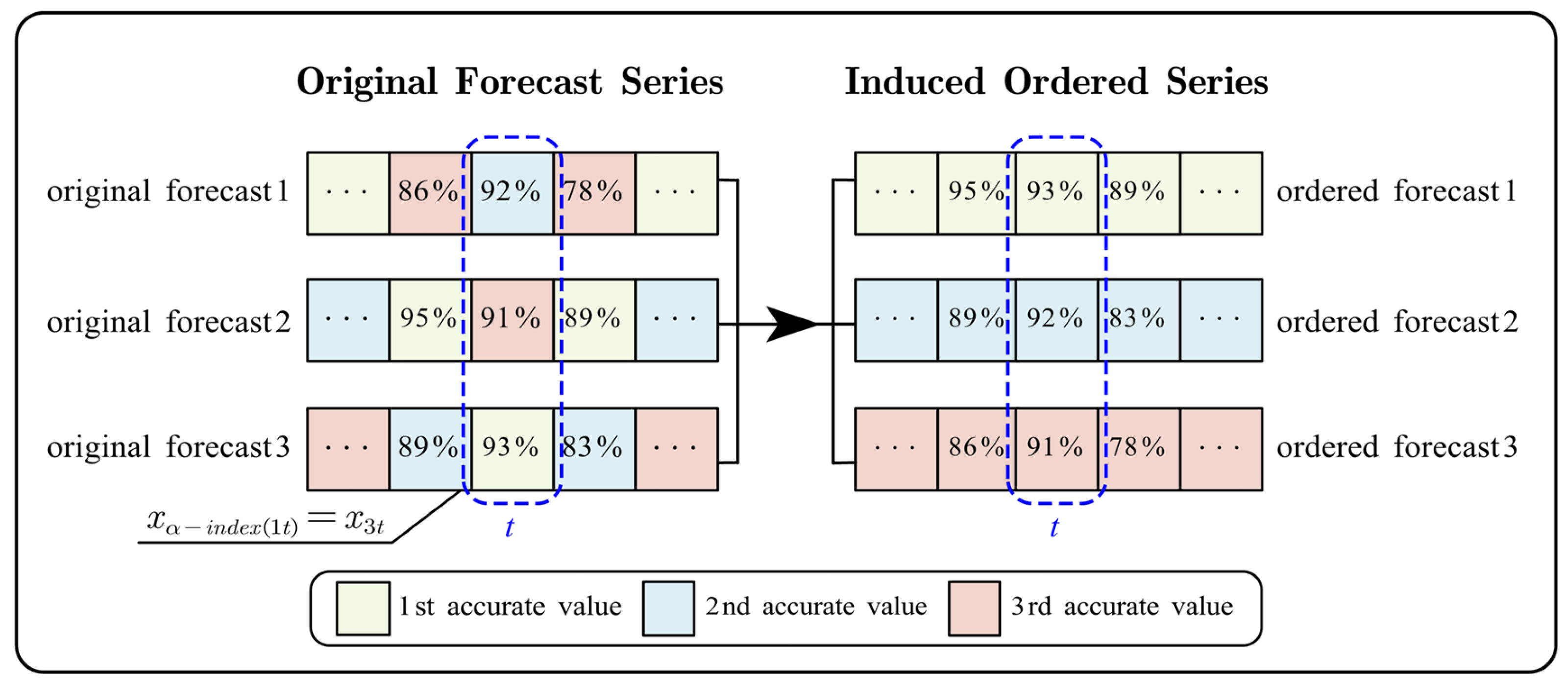
Figure 1. Process of induced ordering in GIOWA combination forecasting.
Mathematics 13 01955 g001
Figure 2. Structure of the LSTM cell.
Mathematics 13 01955 g002
Figure 3. Prediction results of SVR and LSTM models.
Mathematics 13 01955 g003
Figure 4. Forecast errors of SVR and LSTM models.
Mathematics 13 01955 g004
Figure 5. Comparison of the forecast errors across different models.
Mathematics 13 01955 g005
Figure 6. Forecast results of individual models and the GIOWA model.
Mathematics 13 01955 g006
Table 1. Descriptive statistics.
VariablesMeanMaxMinStd. Dev
Construction CO2 emissions (million tons)33.3746.7515.2710.63
Construction workforce (million people)36.6655.3019.9413.10
Urban resident population (million people)656.03914.25394.49163.94
Urbanization rate0.490.650.320.10
TECCI (Mtce)51.9696.0811.7927.57
COPC (kCNY/capita)240.40532.4143.43155.54
Table 2. Error comparison of the individual models and the GIOWA models.
ErrorsSVRLSTMλ = 1λ = −1λ → 0λ = 1/2λ = 1/4
MSE0.9602 2.7804 0.5946 0.5946 0.5910 0.5926 0.5915
MAE0.7362 1.3480 0.5970 0.5964 0.6027 0.5946 0.5944
RMSRE3.26%5.14%2.37%2.37%2.35%2.36%2.36%
MAPE2.40%4.04%1.87%1.87%1.88%1.86%1.86%
Average accuracy97.60%95.96%98.13%98.13%98.12%98.14%98.14%
Table 3. Error comparison of the GIOWA models and other combination forecasting models.
ErrorsSAIVWBMABGOCλ = 1λ = 1/2λ = 1/4
MSE1.0636 0.8078 1.0140 0.8069 0.5946 0.5926 0.5915
MAE0.8258 0.7365 0.7391 0.7391 0.5970 0.5946 0.5944
RMSRE3.22%2.93%2.92%2.92%2.37%2.36%2.36%
MAPE2.55%2.36%2.53%2.37%1.87%1.86%1.86%
Average accuracy97.45%97.64%97.47%97.63%98.13%98.14%98.14%
Table 4. Prediction errors and accuracy of influential factors by DES.
VariablesMAPERMSREAccuracy
Construction workforce3.35%4.44%96.65%
Urban resident population0.49%0.57%99.51%
Urbanization rate0.34%0.39%99.66%
TECCI3.30%4.09%96.70%
Total construction output value1.25%1.39%98.75%
Table 5. Combination weights and forecast values of the GIOWA model for 2022–2030.
Year w 1 w 2 Forecast Value
20220.89200.108038.77
20230.83100.169037.00
20240.77300.227035.41
20250.73400.266033.94
20260.69900.301032.76
20270.66100.339031.83
20280.64800.352031.03
20290.63600.364030.42
20300.62900.371029.99
Disclaimer/Publisher’s Note: The statements, opinions and data contained in all publications are solely those of the individual author(s) and contributor(s) and not of MDPI and/or the editor(s). MDPI and/or the editor(s) disclaim responsibility for any injury to people or property resulting from any ideas, methods, instructions or products referred to in the content.