Event-Triggered Anti-Synchronization of Fuzzy Delay-Coupled Fractional Memristor-Based Discrete-Time Neural Networks

Abstract

This paper investigates the anti-synchronization problem of delay-coupled fractional memristor-based discrete-time neural networks within the T-S fuzzy framework via an event-triggered mechanism. First, fractional-order, coupling topology, and T-S fuzzy rules are incorporated into the discrete-time network model to enhance its applicability. Subsequently, a T-S fuzzy-based event-triggered mechanism is designed, which determines control updates by evaluating whether the system state satisfies predefined triggering conditions, thereby significantly reducing the communication load. Moreover, using diverse fuzzy rules enhances controller flexibility and accuracy. Finally, Zeno behavior is proven to be absent. Using the Lyapunov direct method and inequality techniques, we derive sufficient conditions to ensure anti-synchronization of the proposed system.Numerical simulations confirm the effectiveness of the proposed control scheme and support the theoretical results.

1. Introduction

In recent years, memristor-based neural networks, by replacing the resistive elements in conventional neural networks with memristors, have not only inherited the unique properties of memristors—such as low power consumption, quick switching and nano-scale size [1,2]—but have also demonstrated substantial performance enhancements over traditional architectures. These advancements have unlocked groundbreaking application potential in fields including signal processing, neuromorphic computing, and pattern recognition [3,4,5]. Of particular interest is the anti-synchronization phenomenon, which helps explain the competitive and inhibitory dynamics in memristor-based neural networks and has consequently garnered significant attention from researchers such as Huang and Li [6], Cao et al. [7], and Li et al. [8].

In fact, compared to continuous-time neural networks, discrete-time neural networks (DTNNs) are more amenable to integration with digital circuit technologies due to their discrete update rules. This not only simplifies hardware design but also enhances the efficiency of numerical computations and the stability of parallel processing capabilities [9,10]. Numerous studies have reported achievements in DTNN anti-synchronization. Priyanka and Nagamani [11] addressed the anti-synchronization problem of uncertain DTNNs with time-varying delays within the framework of the complex domain by utilizing an output feedback mechanism. Zhang et al. [12] further considered discrete-time and spatial stochastic delayed inertial DTNNs with adaptive correction parameters, and explored their mean-square anti-synchronization by utilizing a spatiotemporal discrete Lyapunov functional. However, research on anti-synchronization in memristor-based DTNNs (MDTNNs) is still in its nascent stages. Liu et al. [13] innovatively introduced the T-S fuzzy modeling approach—which decomposes complex nonlinear dynamics into a fuzzy weighted combination of local linear subsystems—and, by integrating this approach with impulsive sampling control (ISC) strategies and the Lyapunov functional method, successfully derived rigorous mathematical criteria to ensure anti-synchronization of MDTNNs.

Current research has predominantly focused on integer-order DTNNs. In contrast, fractional-order calculus, owing to its nonlocality and long-term memory properties [14], offers superior accuracy in modeling systems with historical dependence [15]. In recent years, significant progress has been made in fractional DTNNs [16,17,18]. Yang et al. [19] proposed new fractional-order h-difference inequalities and utilized a quantized control mechanism to address the synchronization problem of fractional fuzzy DTNNs. Cui et al. [20] developed a rational novel hybrid controller (HC) to achieve complete synchronization of a class of coupled fractional DTNNs. Zhang et al. [21] further explored the quasi-projection synchronization of fractional DTNNs by leveraging the properties of the Laplace transform, discrete Mittag–Leffler functions, as well as nonlinear feedback control (FC) theory.

Event-triggered mechanisms (ETMs), distinct from impulsive control with its predetermined time-triggered mechanism, is a state-dependent strategy that dynamically activates control based on real-time system status. This approach significantly reduces communication and computational costs [22], leading to its widespread adoption in networked control systems and continued in-depth research attention from academia. For example, Wu et al. [23] developed a static ETM to solve the formation problem of multi-agent systems, while Lu et al. [24] designed a novel quantized ETM to achieve $H_{\infty }$-consensus. However, to date, research on event-triggered anti-synchronization of fractional MDTNNs (FMDTNNs) within the T-S fuzzy logic framework remains unexplored. Moreover, time delays and topological structures, as inherent attributes of networks, directly influence the dynamic characteristics of the system. Designing an efficient ETM using the Lyapunov direct method to achieve anti-synchronization in delay-coupled FMDTNNs remains a challenging open problem.

Based on the aforementioned analysis, this paper aims to tackle the challenge of anti-synchronization in FMDTNNs within the T-S fuzzy framework. The main innovations are as follows: Firstly, by breaking through the limitations of existing works [13], a new delay-coupled FMDTNNs model is established within the T-S fuzzy framework, significantly enhancing the model’s real-world relevance. Secondly, a novel T-S fuzzy ETM (FETM) is innovatively designed, and different fuzzy rules can improve the control performance compared to [24]. Lastly, a new Lyapunov function is constructed, and easily verifiable sufficient conditions are established.

As shown in

Table 1. Comparison of key features with related works.

Features	[13]	[20]	[21]	This Paper
Topology structure	✗	✓	✗	✓
Time delay	✗	✓	✓	✓
T-S fuzzy	✓	✗	✗	✓
Controller	ISC	HC	FC	FETM

, we provide a systematic comparison with recent related works [13,20,21] focusing on four key aspects. The symbols ✓ and ✗ mark whether each item is included.

Notations: ${}^C\nabla _{t_0}^{\mu }$ represents the $\mu$-order ($\mu \in (0,1)$) discrete-time Caputo fractional difference operator. $\mathbb{R}$ denotes the set of real numbers. ${\mathbb{R}}^n$ represents the n-dimensional Euclidean space. ${\mathbb{R}}^{m\times n}$ is the set of all $m\times n$-dimensional real matrices. I represents the identity matrix. $D^T$ stands for the transpose of the matrix D. ⊗ is the Kronecker product. $\mathrm{diag}\{\cdots \}$ denotes a block-diagonal matrix. ${\lambda }_{max}\left(X\right)$ and ${\lambda }_{min}\left(X\right)$ are the maximum eigenvalue and the minimum eigenvalue of the real symmetric matrix X, respectively. $\mathrm{sgn}$ is $\mathrm{sign}$ function. $\parallel ·\parallel$ means the 1 − norm. ${\mathbb{N}}_a=\{a,a+1,a+2,\cdots \}$, ${\mathbb{N}}_a^b=\{a,a+1,a+2,\cdots ,b\}$, and $a-b=\daleth$, $\daleth \in {\mathbb{Z}}^{+}$.

2. Model Description and Preliminaries

2.1. Graph Theory

A weighted digraph $(\mathcal{G},W(t\left)\right)$ consists of the neuron set $\mathcal{N}$ and the matrix $W\left(t\right)={\left(w_{ij}\left(t\right)\right)}_{N\times N}\in {\mathbb{R}}^{N\times N}$. Moreover, $w_{ij}\left(t\right)>0$ if and only if there exists at least one directed edge from neuron j to neuron i; otherwise, $w_{ij}\left(t\right)=0$. The digraph $(\mathcal{G},W(t\left)\right)$ is said to be strongly connected if, for any pair of distinct neurons, there exists a directed path connecting them. The Laplacian matrix of $(\mathcal{G},W(t\left)\right)$ is defined as $L\left(W\left(t\right)\right)={\left(a_{ij}\left(t\right)\right)}_{N\times N}$, where $a_{ij}\left(t\right)=-w_{ij}\left(t\right)$ for $j\ne i$, and $a_{ii}\left(t\right)={\sum }_{k\ne i}{w}_{ik}\left(t\right)$.

2.2. T-S Fuzzy Delay-Coupled FMDTNNs

Consider the following MDTNNs with N neurons and each neuron has n dimensions:

$$\begin{array}{cc}\hfill {}^C\nabla _{k_0}^{\mu }{x}_i\left(k\right)=& -D_i{x}_i\left(k\right)+A\left(x_i\left(k\right)\right)f\left(x_i\left(k\right)\right)+B\left(x_i(k-\tau \left(k\right))\right)f\left(x_i(k-\tau \left(k\right))\right)\hfill \\ & +c\sum _{j=1}^N{\omega }_{ij}\Gamma x_j\left(k\right)+u_i\left(k\right),\hfill \end{array}$$

(1)

where $i=1,2,\cdots ,N$, $x_i\left(k\right)={(x_{i1}\left(k\right),x_i\left(k\right),\dots ,x_{in}\left(k\right))}^T$ is the state of the ith neuron, $D_i=\mathrm{diag}\{d_{i1},d_{i2},\cdots ,d_{in}\}$ denotes the self-feedback connection weight matrix. $f(·)$ is the activation functions, $\tau \left(k\right)$ resprsents the time-varying delay with $0⩽{\tau }_m⩽\tau \left(k\right)⩽{\tau }_M$, ${\tau }_m$ and ${\tau }_M$ are given positive integers $(k\in {\mathbb{N}}_a)$. $A\left(x_i\left(k\right)\right)={\left({\alpha }_{pq}\left(x_{ip}\left(k\right)\right)\right)}_{n\times n}$ and $B\left(x_i(k-\tau \left(k\right))\right)=({\beta }_{pq}{\left(x_{ip}(k-\tau \left(k\right))\right)}_{n\times n}$ are the feedback connection weights and the delayed feedback connection weights, $c>0$ denotes state coupling strength, coupled structure matrix $W={\left({\omega }_{ij}\right)}_{N\times N}$ means that the physical topology satisfies ${\omega }_{ii}=-{\sum }_{j=1,i\ne j}^N{\omega }_{ij}$ and ${\sum }_{i=1,i\ne j}^N{\omega }_{ij}⩾0$, $(j=1,2,\cdots ,N)$, $\Gamma$ is the internal coupling matrix. $u_i\left(k\right)$ is the control input. The initial condition of (1) is given by $x_i\left(t\right)={\gamma }_i\left(t\right)$, $t\in {\mathbb{N}}_{-{\tau }_M}^0$.

The definitions of ${\alpha }_{pq}\left(x_{ip}\left(k\right)\right)$ and ${\beta }_{pq}\left(x_{ip}(k-\tau \left(k\right))\right)$ can be expressed as follows:

$$\begin{array}{cc}\hfill & {\alpha }_{pq}\left(x_{ip}\left(k\right)\right)=\left\{\begin{array}{cc}{\alpha }_{pq}^{*},& x_{ip}\left(k\right)⩽{\daleth }_i,\\ {\alpha }_{pq}^{**},& x_{ip}\left(k\right)>{\daleth }_i,\end{array}\right.\hfill \\ \hfill & {\beta }_{pq}\left(x_{ip}(k-\tau \left(k\right))\right)=\left\{\begin{array}{cc}{\beta }_{pq}^{*},& x_{ip}(k-\tau \left(k\right))⩽{\daleth }_i,\\ {\beta }_{pq}^{**},& x_{ip}(k-\tau \left(k\right))>{\daleth }_i,\end{array}\right.\hfill \end{array}$$

where ${\daleth }_i>0$ is the switching jump, ${\alpha }_{pq}^{*},{\alpha }_{pq}^{**},{\beta }_{pq}^{*}$ and ${\beta }_{pq}^{**}$ are scalar quantities. For the convenience of subsequent analysis, let ${\acute{\alpha }}_{pq}=\max \{{\alpha }_{pq}^{*},{\alpha }_{pq}^{**}\},{\stackrel{‵}{\alpha }}_{pq}=\min \{{\alpha }_{pq}^{*},{\alpha }_{pq}^{**}\},{\widehat{\alpha }}_{pq}={\displaystyle \frac{1}{2}}({\acute{\alpha }}_{pq}+{\stackrel{‵}{\alpha }}_{pq}),{\check{\alpha }}_{pq}={\displaystyle \frac{1}{2}}({\acute{\alpha }}_{pq}-{\stackrel{‵}{\alpha }}_{pq}),{\acute{\beta }}_{pq}=\max \{{\beta }_{pq}^{*},{\beta }_{pq}^{**}\},{\stackrel{‵}{\beta }}_{pq}=\max \{{\beta }_{pq}^{*},{\beta }_{pq}^{**}\},{\widehat{\beta }}_{pq}={\displaystyle \frac{1}{2}}({\acute{\beta }}_{pq}+{\stackrel{‵}{\beta }}_{pq}),{\check{\beta }}_{pq}={\displaystyle \frac{1}{2}}({\acute{\beta }}_{pq}-{\stackrel{‵}{\beta }}_{pq})$.

By introducing (1) into T-S fuzzy logic and applying fuzzy blending, a class of fuzzy delay-coupled FMDTNNs can be derived.

Fuzzy rules ℓ: if $h_1\left(k\right)$ is ${{\rm Y}}_1^{\ell }$, $h_2\left(k\right)$ is ${{\rm Y}}_2^{\ell }$, ⋯, $h_{\chi }\left(k\right)$ is ${{\rm Y}}_{\chi }^{\ell }$$(\ell =1,2,\cdots ,S)$, then

$$\begin{array}{cc}\hfill {}^C\nabla _{k_0}^{\mu }{x}_i\left(k\right)=& \sum _{\ell =1}^S{\eta }_{\ell }\left(h\left(k\right)\right)\{-D_i^{\ell }{x}_i\left(k\right)+A^{\ell }\left(x_i\left(k\right)\right)f\left(x_i\left(k\right)\right)+c\sum _{j=1}^N{\omega }_{ij}\Gamma x_j\left(k\right)\hfill \\ & +u_i\left(k\right)+B^{\ell }\left(x_i(k-\tau \left(k\right))\right)f\left(x_i(k-\tau \left(k\right))\right)\},\hfill \end{array}$$

(2)

where ${{\rm Y}}_l^{\ell }\left(k\right)$$(l=1,2,\cdots ,\chi )$ is the premise variable, the membership function ${\eta }_{\ell }\left(h\left(k\right)\right)$ satisfies

$${\eta }_{\ell }\left(h\left(k\right)\right)={\displaystyle \frac{{\gimel }_{\ell }\left(h\left(k\right)\right)}{{\sum }_{\ell =1}^S{\gimel }_{\ell }\left(h\left(k\right)\right)}},{\gimel }_{\ell }\left(h\left(k\right)\right)=\prod _{l=1}^{\chi }{{\rm Y}}_l^{\ell }\left(h_l\left(k\right)\right),$$

where ${{\rm Y}}_l^{\ell }\left(h_l\left(k\right)\right)$ denotes the grade of membership of $h_l\left(k\right)$ on the fuzzy set ${{\rm Y}}_l^{\ell }$ and ${\eta }_{\ell }\left(h\left(k\right)\right)$ satisfies the following conditions

$${\eta }_{\ell }\left(h\left(k\right)\right)⩾0,\sum _{\ell =1}^S{\eta }_{\ell }\left(h\left(k\right)\right)=1.$$

Next, we need to introduce some new variables, as $A={\left({\widehat{\alpha }}_{ij}\right)}_{n\times n},B={\left({\widehat{\beta }}_{ij}\right)}_{n\times n}$, according to the Kronecker product, the system (1) can be rewritten in the following form

$$\begin{array}{cc}\hfill {}^C\nabla _{k_0}^{\mu }x\left(k\right)=& \sum _{\ell =1}^S{\eta }_{\ell }\left(h\left(k\right)\right)\{-(I_N\otimes D^{\ell })x\left(k\right)+(I_N\otimes A^{\ell }+I_N\otimes M_{\alpha }{\Lambda }_1^{\ell }\left(k\right)N_{\alpha })f\left(x\left(k\right)\right)\hfill \\ \hfill & +(I_N\otimes B^{\ell }+I_N\otimes M_{\beta }{\Lambda }_2^{\ell }\left(k\right)N_{\beta })f\left(x(k-\tau \left(k\right))\right)+c(W\otimes \Gamma )x\left(k\right)+u\left(k\right)\},\hfill \end{array}$$

(3)

where

$$\begin{array}{cc}\hfill & M_{\alpha }={(\sqrt{{\check{\alpha }}_{11}}{\nu }_1,\dots ,\sqrt{{\check{\alpha }}_{1n}}{\nu }_n,\dots ,\sqrt{{\check{\alpha }}_{n1}}{\nu }_1,\dots ,\sqrt{{\check{\alpha }}_{nn}}{\nu }_n)}_{n\times n^2},\hfill \\ \hfill & N_{\alpha }={(\sqrt{{\check{\alpha }}_{11}}{\nu }_1,\dots ,\sqrt{{\check{\alpha }}_{1n}}{\nu }_n,\dots ,\sqrt{{\check{\alpha }}_{n1}}{\nu }_1,\dots ,\sqrt{{\check{\alpha }}_{nn}}{\nu }_n)}_{n^2\times n}^T,\hfill \\ \hfill & M_{\beta }={(\sqrt{{\check{\beta }}_{11}}{\nu }_1,\dots ,\sqrt{{\check{\beta }}_{1n}}{\nu }_1,\dots ,\sqrt{{\check{\beta }}_{n1}}{\nu }_n,\dots ,\sqrt{{\check{\beta }}_{nn}}{\nu }_n)}_{n\times n^2},\hfill \\ \hfill & N_{\beta }={(\sqrt{{\check{\beta }}_{11}}{\nu }_1,\dots ,\sqrt{{\check{\beta }}_{1n}}{\nu }_n,\dots ,\sqrt{{\check{\beta }}_{n1}}{\nu }_1,\dots ,\sqrt{{\check{\beta }}_{nn}}{\nu }_n)}_{n^2\times n}^T,\hfill \\ \hfill & {\Lambda }_r\left(k\right)=\mathrm{diag}\{{\Lambda }_{11}^r\left(k\right),\dots ,{\Lambda }_{1n}^r\left(k\right),\dots ,{\Lambda }_{n1}^r\left(k\right),\dots ,{\Lambda }_{nn}^r\left(k\right)\}\in {\mathbb{R}}^{n^2\times n^2},\hfill \end{array}$$

where ${\nu }_i\in {\mathbb{R}}^n$ represents the column vector with ith element being one while the other elements are zero. It can be easily shown that ${\Lambda }_r^T\left(k\right){\Lambda }_r\left(k\right)⩽I$, for $r=1,2,3,4$.

We consider (1) as the response system, the following drive system is chosen as

$$\begin{array}{cc}\hfill {}^C\nabla _{k_0}^{\mu }{y}_i\left(k\right)=& \sum _{\ell =1}^S{\eta }_{\ell }\left(h\left(k\right)\right)\{-D_i^{\ell }{y}_i\left(k\right)+A^{\ell }\left(y_i\left(k\right)\right)f\left(y_i\left(k\right)\right)+c\sum _{j=1}^N{\omega }_{ij}\Gamma y_j\left(k\right)\hfill \\ & +B^{\ell }\left(y_i(k-\tau \left(k\right))\right)f\left(y_i(k-\tau \left(k\right))\right)\},\hfill \end{array}$$

(4)

where $A\left(y_i\left(k\right)\right)={\left({\alpha }_{pq}\left(y_{ip}\left(k\right)\right)\right)}_{n\times n}$ and $B\left(y_i(k-\tau \left(k\right))\right)=({\beta }_{pq}{\left(y_{ip}(k-\tau \left(k\right))\right)}_{n\times n}$ are the feedback connection weights and the delayed feedback connection weights. The initial condition of drive system (4) is selected by $y\left(t\right)={\gamma }_0\left(t\right)$, $t\in {\mathbb{N}}_{-{\tau }_M}^0$.

The definitions of ${\alpha }_{pq}\left(y_{ip}\left(k\right)\right)$ and ${\beta }_{pq}\left(y_{ip}(k-\tau \left(k\right))\right)$ can be expressed as follows:

$$\begin{array}{cc}\hfill & {\alpha }_{pq}\left(y_i\left(k\right)\right)=\left\{\begin{array}{cc}{\alpha }_{pq}^{*},& y_{ip}\left(k\right)⩽{\daleth }_i,\\ {\alpha }_{pq}^{**},& y_{ip}\left(k\right)>{\daleth }_i,\end{array}\right.\hfill \\ \hfill & {\beta }_{pq}\left(y_{ip}(k-\tau \left(k\right))\right)=\left\{\begin{array}{cc}{\beta }_{pq}^{*},& y_{ip}(k-\tau \left(k\right))⩽{\daleth }_i,\\ {\beta }_{pq}^{**},& y_{ip}(k-\tau \left(k\right))>{\daleth }_i.\end{array}\right.\hfill \end{array}$$

Then, the drive system can be denoted as

$$\begin{array}{cc}\hfill {}^C\nabla _{k_0}^{\mu }y\left(k\right)=& \sum _{\ell =1}^S{\eta }_{\ell }\left(h\left(k\right)\right)\{-(I_N\otimes D^{\ell })y\left(k\right)+(I_N\otimes A^{\ell }+I_N\otimes M_{\alpha }{\Lambda }_3^{\ell }\left(k\right)N_{\alpha })f\left(y\left(k\right)\right)\hfill \\ \hfill & +(I_N\otimes B^{\ell }+I_N\otimes M_{\beta }{\Lambda }_4^{\ell }\left(k\right)N_{\beta })f\left(y(k-\tau \left(k\right))\right)+c(W\otimes \Gamma )y\left(k\right)\}.\hfill \end{array}$$

(5)

Remark 1.

The model in [13] neglects the coupling topology among nodes and fails to take into account the modeling advantages of fractional order. The model studied in this paper is more in line with practical MDTNNs. Moreover, to the best of our knowledge, no research has addressed the issue of FMDTNNs with delay-coupling topology within the T-S fuzzy framework, which underscores the significance of our study.

Defining the error vector as $e\left(k\right)=x\left(k\right)+y\left(k\right)$, $g\left(e\right(k\left)\right)=f\left(x\right(k\left)\right)+f\left(y\right(k\left)\right)$, the error system can be written as follows

$$\begin{array}{cc}\hfill {}^C\nabla _{k_0}^{\mu }e\left(k\right)=& \sum _{\ell =1}^S{\eta }_{\ell }\left(h\left(k\right)\right)\{-(I_N\otimes D^{\ell })e\left(k\right)+(I_N\otimes A^{\ell }+I_N\otimes M_{\alpha }{\Lambda }_3^{\ell }\left(k\right)N_{\alpha })g\left(e\left(k\right)\right)\hfill \\ \hfill & +(I_N\otimes B^{\ell }+I_N\otimes M_{\beta }{\Lambda }_4^{\ell }\left(k\right)N_{\beta })g\left(e(k-\tau \left(k\right))\right)\hfill \\ \hfill & +(I_N\otimes M_{\alpha }({\Lambda }_1^{\ell }\left(k\right)-{\Lambda }_3^{\ell }\left(k\right))N_{\alpha })f\left(x\left(k\right)\right)\hfill \\ \hfill & +(I_N\otimes M_{\beta }({\Lambda }_2^{\ell }\left(k\right)-{\Lambda }_4^{\ell }\left(k\right))N_{\beta })f\left(x(k-\tau \left(k\right))\right)\hfill \\ \hfill & +c(W\otimes \Gamma )e\left(k\right)+u\left(k\right)\}.\hfill \end{array}$$

(6)

Assumption 1

([25]). The activation function $f_i(·)$ is continuous and satisfies

$$|f_i\left(x\right)+f_i\left(y\right)|⩽h_i|x+y|,|f_i\left(x\right)|⩽l_i,$$

where $h_i>0$ and $l_i>0$ are constants.

Definition 1

([26]). For $\mu \ne -1,-2,-3,\cdots$, the rising factorial function $t^{\overline{\mu }}$ is depicted as

$$t^{\overline{\mu }}={\displaystyle \frac{\Gamma (t+\mu )}{\Gamma \left(t\right)}},t\in \mathbb{R}-\{\cdots ,-2,-1,0\},$$

where $\Gamma \left(\xi \right)={\int }_0^{\infty }{e}^{-\eta }{\eta }^{\xi -1}d\eta$.

Definition 2

([27]). Given a function ${\rm Y}:{\mathbb{N}}_a\to \mathbb{R}$, one can represent the μ ($\mu \in (0,1)$) order Caputo-like Nabla fractional difference of function ${\rm Y}\left(t\right)$ as

$$\begin{array}{cc}\hfill {}^C\nabla _a^{\mu }{\rm Y}\left(t\right)& ={\nabla }_a^{-(1-\mu )}\nabla {\rm Y}\left(t\right)\hfill \\ \hfill & ={\displaystyle \frac{1}{\Gamma (1-\mu )}}\sum _{s=a+1}^t{(t-\rho \left(s\right))}^{\overline{-\mu }}\nabla {\rm Y}\left(s\right),t\in {\mathbb{N}}_{a+1},\hfill \end{array}$$

where $\rho \left(s\right)=s-1$, $\nabla {\rm Y}\left(t\right)={\rm Y}\left(t\right)-{\rm Y}(t-1)$ is the backward difference operator of ${\rm Y}\left(t\right)$ and ${\nabla }^h{\rm Y}\left(t\right)=\nabla \left({\nabla }^{(h-1)}\right){\rm Y}\left(t\right)$. Furthermore, $\nabla \left(t^{\overline{\mu }}\right)=\mu t^{\mu -1}$.

Definition 3

([28]). For $\widehat{\lambda }\in \mathbb{R},|\widehat{\lambda }|<1,$ and $\alpha ,\gamma \in \mathbb{R},$ the Nabla discrete Mittag–Leffler function with two parameters is defined as

$$E_{\overline{\alpha ,\gamma }}(\widehat{\lambda },t)=\sum _{k=0}^{\infty }{\widehat{\lambda }}^k{\displaystyle \frac{t^{\overline{k\alpha +\gamma -1}}}{\Gamma (k\alpha +\gamma )}}.$$

In particularly, for $\gamma =1$, one has

$$E_{\overline{\alpha }}(\widehat{\lambda },t)=\sum _{k=0}^{\infty }{\widehat{\lambda }}^k{\displaystyle \frac{t^{\overline{k\alpha }}}{\Gamma (k\alpha +1)}}.$$

Definition 4

([28]). Given a function $\xi :{\mathbb{N}}_a\to \mathbb{R}$ and a constant $\mu >0$, the μ-th order sum of $\xi \left(t\right)$ whose starting point is a has the following form

$${\nabla }_a^{-\mu }\xi \left(t\right)={\int }_a^t{\mathcal{H}}_{\mu -1}(t,\rho \left(s\right))\xi \left(s\right){\nabla }_s=\sum _{s=a+1}^t{\displaystyle \frac{{(t-\rho \left(s\right))}^{\overline{\mu -1}}}{\Gamma \left(\mu \right)}}\xi \left(s\right),$$

where $t\in {\mathbb{N}}_{a+1}$, $\rho \left(s\right)=s-1$.

Lemma 1

([21]). Suppose that $\xi \left(k\right)$ is non-negative function and $0<\mu <1$, such that

$${}^C\nabla _0^{\mu }\Psi \left(k\right)⩽-\widehat{p}\xi \left(k\right),k\in {\mathbb{N}}_0,$$

(7)

if ${\displaystyle \frac{1}{2}}<\widehat{p}<{\displaystyle \frac{3}{2}}$, then,

$$\xi \left(k\right)⩽\xi \left(0\right)E_{\mu }(-(\widehat{p}-{\displaystyle \frac{1}{2}}),k).$$

(8)

Lemma 2

([26]). Let the function vector $\ell \left(t\right)={({\ell }_1\left(t\right),\dots ,{\ell }_N\left(t\right))}^T\in {\mathbb{R}}^N$ then for any time instant $t\in {\mathbb{N}}_{a+1}$,

$${\displaystyle \frac{1}{2}}{}^C\nabla _a^{\mu }{\ell }^T\left(t\right)\ell \left(t\right)\le {\ell }^T{\left(t\right)}^C{\nabla }_a^{\mu }\ell \left(t\right),\mu \in (0,1).$$

Lemma 3

([26]). Given a function $\xi :{\mathbb{N}}_a\to \mathbb{R}$ and a constant $\mu >0$ as well as a positive integer number $\mathfrak{h}=\lfloor \mu \rfloor +1$, one has

$${\nabla }_a^{-(\mathfrak{h}-\mu )C}{\nabla }_a^{(\mathfrak{h}-\mu )}\xi \left(t\right)=\xi \left(t\right)-\xi \left(a\right).$$

3. Main Results

This section focuses on anti-synchronization of delay-coupled FMDTNNs by ETM, which can be discussed in the following theorems.

3.1. Fuzzy Event-Triggered Mechanism

To synchronize the drive-response system, the event-triggered aperiodic intermittent mechanism $u_i\left(k\right)$ is designed as follows:

$$u_i\left(k\right)=K_i{e}_i\left(k_s^i\right)-{\displaystyle \frac{Q_i\mathrm{sgn}\left(e_i\left(k_s^i\right)\right)}{\parallel e\left(k_s^i\right)\parallel }},$$

(9)

where $K_i$ and $Q_i$ are the control feedback gain matrix and $k_s^i$ represents the sth triggered instant of the ith node.

Fuzzy rule $\varsigma$: if $v_1\left(k\right)$ is ${\varpi }_1^{\varsigma }$, $v_2\left(k\right)$ is ${\varpi }_2^{\varsigma }$, ⋯, $v_L\left(k\right)$ is ${\varpi }_L^{\varsigma }$$(\varsigma =1,2,\cdots ,L)$, then, by the fuzzy blending, the controller with fuzziness can be rewritten as

$$u_i\left(k\right)=\begin{array}{c}\hfill \sum _{\varsigma =1}^L{\psi }_{\varsigma }\left(v\left(k\right)\right)[K_i^{\varsigma }{e}_i\left(k_s^i\right)-{\displaystyle \frac{Q_i\mathrm{sgn}\left(e_i\left(k_s^i\right)\right)}{\parallel e\left(k_s^i\right)\parallel }}],\end{array}$$

(10)

where

$${\psi }_{\varsigma }\left(v\left(k\right)\right)={\displaystyle \frac{{\daleth }_{\varsigma }\left(v\left(k\right)\right)}{{\sum }_{\varsigma =1}^S{\daleth }_{\varsigma }\left(\left(k\right)\right)}},{\daleth }_{\varsigma }\left(v\left(k\right)\right)=\prod _{\mathfrak{l}=1}^L{\varpi }_{\mathfrak{l}}^{\varsigma }\left(v_{\mathfrak{l}}\left(k\right)\right),$$

in which ${\varpi }_{\mathfrak{l}}^{\varsigma }\left(v_{\mathfrak{l}}\left(k\right)\right)$ denotes the grade of membership of $v_{\mathfrak{l}}\left(k\right)$ on the fuzzy set ${\varpi }_{\mathfrak{l}}^{\varsigma }$ and ${\psi }_{\varsigma }\left(v\left(k\right)\right)$ satisfies the following conditions

$${\psi }_{\varsigma }\left(v\left(k\right)\right)⩾0,\sum _{\varsigma =1}^R{\psi }_{\varsigma }\left(v\left(k\right)\right)=1.$$

Remark 2.

The introduction of T-S fuzzy rules differing from the system into the control mechanism (12) enhances the flexibility and robustness of control mechanism design, enabling better adaptation to system uncertainties and complex dynamics, thereby achieving more efficient and precise synchronous control.

To reduce the frequency of controller updates, this article uses ETM to decide whether to send the current data. The sequence that triggers the moment can be expressed as $0⩽k_0^i<k_1^i<\cdots <k_s^i<\cdots$, then $k_{s+1}^i$ is denoted by

$$k_{s+1}^i=\min \{k\in \mathbb{N}:k>k_s^i,\varrho e_i^T\left(k\right)e_i\left(k\right)<{\xi }_i^T\left(k\right){\xi }_i\left(k\right)\},$$

(11)

where $\varrho \in (0,{\displaystyle \frac{1}{2}})$ is given scalars, and ${\xi }_i\left(k\right)=e_i\left(k_s^i\right)-e_i\left(k\right)$ is used to control the state error between input updates.

3.2. Main Theorem

By combining (6) and (10), the following dynamic error system can be obtained:

$$\begin{array}{cc}\hfill {}^C\nabla _{k_0}^{\mu }e\left(k\right)=& \sum _{\ell =1}^S\sum _{\varsigma =1}^R{\eta }_{\ell }\left(h\left(k\right)\right){\psi }_{\varsigma }\left(v\left(k\right)\right)\{-(I_N\otimes D^{\ell })e\left(k\right)\hfill \\ \hfill & +(I_N\otimes {\overline{A}}^{\ell })g\left(e\left(k\right)\right)+(I_N\otimes {\overline{B}}^{\ell })g\left(e(k-\tau \left(k\right))\right)\hfill \\ \hfill & +(I_N\otimes {\overline{M}}_1)f\left(y\left(k\right)\right)+(I_N\otimes {\overline{M}}_2)f\left(y(k-\tau \left(k\right))\right)\hfill \\ \hfill & +c(W\otimes \Gamma )e\left(k\right)+(K^{\varsigma }\otimes I_n)(e\left(k\right)+\xi \left(k\right))\hfill \\ \hfill & -(Q\otimes I_n){\displaystyle \frac{\mathrm{sgn}\left(e\right(k)+\xi (k\left)\right)}{\parallel e\left(k\right)+\xi \left(k\right)\parallel }}\},\hfill \end{array}$$

(12)

in which ${\overline{A}}^{\ell }=A^{\ell }+M_{\alpha }{\Lambda }_3^{\ell }\left(k\right)N_{\alpha }$, ${\overline{B}}^{\ell }=B^{\ell }+M_{\beta }{\Lambda }_3^{\ell }\left(k\right)N_{\beta }$, ${\overline{M}}_1=M_{\alpha }({\Lambda }_1^{\ell }\left(k\right)-{\Lambda }_3^{\ell }\left(k\right))N_{\alpha })$, ${\overline{M}}_2=M_{\beta }({\Lambda }_2^{\ell }\left(k\right)-{\Lambda }_4^{\ell }\left(k\right))N_{\beta }$.

Theorem 1.

Let Assumption 1 be satisfied. If there exist constants δ, ${\delta }^{\prime }$, ϑ and σ such that

$$\left\{\begin{array}{cc}\hfill \delta =& {\lambda }_{min}\left({\Omega }_1\right)>0,\hfill \\ \hfill \vartheta =& {\lambda }_{max}(I_N\otimes {\mathcal{H}}^T\mathcal{H})>0,\hfill \\ \hfill \sigma =& {\lambda }_{min}(2I_N\otimes {\mathcal{L}}^T\mathcal{L}+2{\varrho }^{\prime }(Q^{\prime }\otimes I_n))<0,\hfill \\ \hfill {\delta }^{\prime }=& \delta -\iota \vartheta \in ({\displaystyle \frac{1}{2}},{\displaystyle \frac{3}{2}}),\hfill \end{array}\right.$$

(13)

where $\Omega ={\sum }_{\ell =1}^S{\sum }_{\varsigma =1}^R{\eta }_{\ell }\left(h\left(k\right)\right){\psi }_{\varsigma }\left(v\left(k\right)\right)\{2I_N\otimes D^{\ell }-I_N\otimes {\overline{A}}^{\ell }{\overline{A}}^{{\ell }^T}-I_N\otimes {\mathcal{H}}^T\mathcal{H}-I_N\otimes {\overline{B}}^{\ell }{\overline{B}}^{{\ell }^T}-I_N\otimes {\overline{M}}_1{\overline{M}}_1^T-I_N\otimes {\overline{M}}_2{\overline{M}}_2^T-2K^{\varsigma }\otimes I_n-2c(W\otimes \Gamma )-K^{\varsigma }{K}^{{\varsigma }^T}\otimes I_n-\varrho \otimes I_{Nn}\}$. ${\Omega }_1={\displaystyle \frac{1}{2}}(\Omega +{\Omega }^T)$ and $Q^{\prime }={\displaystyle \frac{1}{2}}(Q+Q^T)$ are real symmetric matrices. $\iota >1$ is a constant, $\mathcal{H}=\mathrm{diag}\{{\mathrm{h}}_1,{\mathrm{h}}_2,\cdots ,{\mathrm{h}}_{\mathrm{n}}\}$, $\mathcal{L}=\mathrm{diag}\{{\mathrm{l}}_1,{\mathrm{l}}_2,\cdots ,{\mathrm{l}}_{\mathrm{n}}\}$, then, under the fuzzy-based ETM, the systems (2) and (4) can achieve anti-synchronization.

Proof. 

The appropriate Lyapunov auxiliary functional is built as follows:

$$V\left(k\right)=e^T\left(k\right)e\left(k\right).$$

Based on Lemma 2, calculate the difference of $V\left(k\right)$, as follows:

$$\begin{array}{cc}\hfill {}^C\nabla _{k_0}^{\mu }V\left(k\right)⩽& 2e^T\left(k\right){}^C\nabla _{t_0}^{\mu }e\left(k\right)\hfill \\ \hfill ⩽& 2\sum _{\ell =1}^S\sum _{\varsigma =1}^R{\eta }_{\ell }\left(h\left(k\right)\right){\psi }_{\varsigma }\left(v\left(k\right)\right)e^T\left(k\right)\{-(I_N\otimes D^{\ell })e\left(k\right)+(I_N\otimes {\overline{A}}^{\ell })g\left(e\left(k\right)\right)\hfill \\ \hfill & +(I_N\otimes {\overline{B}}^{\ell })g\left(e(k-\tau \left(k\right))\right)+(I_N\otimes {\overline{M}}_1)f\left(y\left(k\right)\right)\hfill \\ \hfill & +(I_N\otimes {\overline{M}}_2)f\left(y(k-\tau \left(k\right))\right)+c(W\otimes \Gamma )e\left(k\right)\hfill \\ \hfill & +(K^{\varsigma }\otimes I_n)(e\left(k\right)-\xi \left(k\right))\hfill \\ \hfill & -(Q\otimes I_n){\displaystyle \frac{\mathrm{sgn}\left(\mathrm{e}\right(\mathrm{k})+\xi (\mathrm{k}\left)\right)}{\parallel e\left(k\right)+\xi \left(k\right)\parallel }}\}.\hfill \end{array}$$

(14)

According to Assumption 1, it is revealed that

$$\begin{array}{c}2e^T\left(k\right)(I_N\otimes {\overline{A}}^{\ell })g\left(e\left(k\right)\right)\hfill \\ =e^T\left(k\right)(I_N\otimes {\overline{A}}^{\ell }){(I_N\otimes {\overline{A}}^{\ell })}^{T}e\left(k\right)+g^T\left(e\left(k\right)\right)g\left(e\left(k\right)\right)\hfill \\ -{[{(I_N\otimes {\overline{A}}^{\ell })}^{T}e\left(k\right)-g^T\left(e\left(k\right)\right)]}^T[{(I_N\otimes {\overline{A}}^{\ell })}^{T}e\left(k\right)-g^T\left(e\left(k\right)\right)]\hfill \\ ⩽e^T\left(k\right)(I_N\otimes {\overline{A}}^{\ell }){(I_N\otimes {\overline{A}}^{\ell })}^{T}e\left(k\right)+g^T\left(e\left(k\right)\right)g\left(e\left(k\right)\right)\hfill \\ ⩽e^T\left(k\right)(I_N\otimes {\overline{A}}^{\ell }){(I_N\otimes {\overline{A}}^{\ell })}^{T}e\left(k\right)+e^T\left(k\right){(I_N\otimes \mathcal{H})}^T(I_N\otimes \mathcal{H})e\left(k\right)\hfill \\ ⩽e^T\left(k\right)(I_N\otimes {\overline{A}}^{\ell }{\overline{A}}^{{\ell }^T}+I_N\otimes {\mathcal{H}}^T\mathcal{H})e\left(k\right).\hfill \end{array}$$

(15)

Then, by a similar derivation, one can arrive at the conclusion that

$$\begin{array}{c}2e^T\left(k\right)(I_N\otimes {\overline{B}}^{\ell })g\left(e(k-\tau \left(k\right))\right)\hfill \\ ⩽e^T\left(k\right)(I_N\otimes {\overline{B}}^{\ell }){(I_N\otimes {\overline{B}}^{\ell })}^{T}e\left(k\right)+g^T\left(e(k-\tau \left(k\right))\right)g\left(e(k-\tau \left(k\right))\right)\hfill \\ ⩽e^T\left(k\right)(I_N\otimes {\overline{B}}^{\ell }){(I_N\otimes {\overline{B}}^{\ell })}^{T}e\left(k\right)+e^T(k-\tau \left(k\right)){(I_N\otimes \mathcal{H})}^T(I_N\otimes \mathcal{H})e(k-\tau \left(k\right))\hfill \\ ⩽e^T\left(k\right)(I_N\otimes {\overline{B}}^{\ell }{\overline{B}}^{{\ell }^T})e\left(k\right)+e^T(k-\tau \left(k\right))(I_N\otimes {\mathcal{H}}^T\mathcal{H})e(k-\tau \left(k\right)).\hfill \end{array}$$

(16)

$$\begin{array}{c}2e^T\left(k\right)(I_N\otimes {\overline{M}}_1)f\left(y\left(k\right)\right)\hfill \\ ⩽e^T\left(k\right)(I_N\otimes {\overline{M}}_1){(I_N\otimes {\overline{M}}_1)}^{T}e\left(k\right)+f^T\left(y\left(k\right)\right)f\left(y\left(k\right)\right)\hfill \\ ⩽e^T\left(k\right)(I_N\otimes {\overline{M}}_1){(I_N\otimes {\overline{M}}_1)}^{T}e\left(k\right)+{(I_N\otimes \mathcal{L})}^T(I_N\otimes \mathcal{L})\hfill \\ ⩽e^T\left(k\right)(I_N\otimes {\overline{M}}_1{\overline{M}}_1^T)e\left(k\right)+I_N\otimes {\mathcal{L}}^T\mathcal{L}.\hfill \end{array}$$

(17)

$$\begin{array}{c}2e^T\left(k\right)(I_N\otimes {\overline{M}}_2)f\left(y(k-\tau \left(k\right))\right)\hfill \\ ⩽e^T\left(k\right)(I_N\otimes {\overline{M}}_2){(I_N\otimes {\overline{M}}_2)}^{T}e\left(k\right)+f^T\left(y(k-\tau \left(k\right))\right)f\left(y(k-\tau \left(k\right))\right)\hfill \\ ⩽e^T\left(k\right)(I_N\otimes {\overline{M}}_2{\overline{M}}_2^T)e\left(k\right)+I_N\otimes {\mathcal{L}}^T\mathcal{L}.\hfill \end{array}$$

(18)

Based on ETM (11), and considering that $\varrho e_i^T\left(k\right)e_i\left(k\right)⩾{\xi }_i^T\left(k\right){\xi }_i\left(k\right)$, one has

$$\begin{array}{c}2e^T\left(k\right)(K^{\varsigma }\otimes I_n)(e\left(k\right)+\xi \left(k\right))\hfill \\ =2e^T\left(k\right)(K^{\varsigma }\otimes I_n)e\left(k\right)+2e^T\left(k\right)(K^{\varsigma }\otimes I_n)\xi \left(k\right)\hfill \\ ⩽2e^T\left(k\right)(K^{\varsigma }\otimes I_n)e\left(k\right)+{\xi }^T\left(k\right){\xi }^T\left(k\right)+e^T\left(k\right)(K^{\varsigma }\otimes I_n){(K^{\varsigma }\otimes I_n)}^{T}e\left(k\right)\hfill \\ ⩽2e^T\left(k\right)(K^{\varsigma }\otimes I_n)e\left(k\right)+e^T\left(k\right)(\varrho \otimes I_{Nn})e\left(k\right)+e^T\left(k\right)(K^{\varsigma }{K}^{{\varsigma }^T}\otimes I_n)e\left(k\right)\hfill \\ ⩽e^T\left(k\right)(2K^{\varsigma }\otimes I_n+\varrho \otimes I_{Nn}+K^{\varsigma }{K}^{{\varsigma }^T}\otimes I_n)e\left(k\right).\hfill \end{array}$$

(19)

$$\begin{array}{cc}\hfill & -2e^T\left(k\right)(Q\otimes I_n){\displaystyle \frac{\mathrm{sgn}\left(\mathrm{e}\right(\mathrm{k})+\xi (\mathrm{k}\left)\right)}{\parallel e\left(k\right)+\xi \left(k\right)\parallel }}\hfill \\ \hfill =& -2{(e\left(k\right)+\xi \left(k\right))}^T(Q\otimes I_n){\displaystyle \frac{\mathrm{sgn}\left(\mathrm{e}\right(\mathrm{k})+\xi (\mathrm{k}\left)\right)}{\parallel e\left(k\right)+\xi \left(k\right)\parallel }}+2{\xi }^T\left(k\right)(Q\otimes I_n){\displaystyle \frac{\mathrm{sgn}\left(\mathrm{e}\right(\mathrm{k})+\xi (\mathrm{k}\left)\right)}{\parallel e\left(k\right)+\xi \left(k\right)\parallel }}\hfill \\ \hfill ⩽& -2(Q\otimes I_n)+2(Q\otimes I_n){\displaystyle \frac{\varrho \parallel e\left(k\right)\parallel }{\parallel e\left(k\right)\parallel -\parallel \xi \left(k\right)\parallel }}\hfill \\ \hfill ⩽& -2(Q\otimes I_n)+2(Q\otimes I_n){\displaystyle \frac{\varrho \parallel e\left(k\right)\parallel }{(1-\varrho )\parallel e\left(k\right)\parallel }}\hfill \\ \hfill ⩽& 2{\varrho }^{\prime }(Q\otimes I_n),\hfill \end{array}$$

(20)

where ${\varrho }^{\prime }={\displaystyle \frac{2\varrho -1}{1-\varrho }}$.

Combined with (15)–(20), it is concluded that

$$\begin{array}{cc}\hfill {}^C\nabla _{k_0}^{\mu }V\left(k\right)⩽& \sum _{\ell =1}^S\sum _{\varsigma =1}^R{\eta }_{\ell }\left(h\left(k\right)\right){\psi }_{\varsigma }\left(v\left(k\right)\right)e^T\left(k\right)[-2I_N\otimes D^{\ell }+I_N\otimes {\overline{A}}^{\ell }{\overline{A}}^{{\ell }^T}\hfill \\ & +I_N\otimes {\mathcal{H}}^T\mathcal{H}+I_N\otimes {\overline{B}}^{\ell }{\overline{B}}^{{\ell }^T}+I_N\otimes {\overline{M}}_1{\overline{M}}_1^T\hfill \\ \hfill & +I_N\otimes {\overline{M}}_2{\overline{M}}_2^T+2K^{\varsigma }\otimes I_n+2c(W\otimes \Gamma )\hfill \\ \hfill & +K^{\varsigma }{K}^{{\varsigma }^T}\otimes I_n+\varrho \otimes I_{Nn}]e\left(k\right)\hfill \\ \hfill & +e^T(k-\tau \left(k\right))(I_N\otimes {\mathcal{H}}^T\mathcal{H})e(k-\tau \left(k\right))\hfill \\ \hfill & +2I_N\otimes {\mathcal{L}}^T\mathcal{L}+2{\varrho }^{\prime }(Q_i\otimes I_n)\hfill \\ \hfill ⩽& -\delta V\left(k\right)+\vartheta V(k-\tau (k\left)\right)\hfill \\ \hfill ⩽& -{\delta }^{\prime }V\left(k\right).\hfill \end{array}$$

(21)

In light of Lemma 1, one may draw the following conclusion

$$V\left(k\right)⩽V\left(0\right)E_{\mu }(-({\delta }^{\prime }-{\displaystyle \frac{1}{2}}),k).$$

Thus,

$$\underset{k\to +\infty }{lim}\parallel y\left(k\right)+x\left(k\right)\parallel =0,$$

which implies augmented error systems (2) and (4) can realize anti-synchronization and the proof is completed. □

Remark 3.

In existing studies, Huang et al. [6] and Cao et al. [7] have all focused on the anti-synchronization control problem of delayed memristor-based neural networks, but their analytical frameworks are limited to the continuous-time domain. Although Cui et al. [20] and Li et al. [21] have extended their research to the synchronization of fractional DTNNs, the conventional feedback control mechanisms they employ suffer from insufficient resource utilization. In contrast, the ETM proposed in this paper achieves efficient allocation of control resources.

3.3. Mitigate the Zeno Phenomenon

Theorem 2.

Under the conditions specified in Theorem 1, the error system (6) governed by the controller (9) and ETM (11) can be ensured to operate without Zeno behavior.

Proof. 

For $k\in [k_s,k_{s+1})$, based on Definition 4 and Lemma 3, one has

$$\begin{array}{cc}\hfill {\parallel \xi \left(k\right)\parallel }_1=& \parallel e\left(k_s\right)-e\left(k\right){\parallel }_1\hfill \\ \hfill =& \parallel {\nabla }_{k_s}^{-\mu }{}^C\nabla _{k_s}^{\mu }{e\left(k\right)\parallel }_1\hfill \\ \hfill =& \parallel {\int }_{k_s}^k{\mathcal{H}}_{\mu -1}(k,\rho \left(s\right)){}^C\nabla _{k_s}^{\mu }e\left(t\right){\nabla }_t{\parallel }_1.\hfill \end{array}$$

(22)

According to Theorem 1, it can be concluded that $e\left(t\right)$ and ${}^C\nabla _{k_s}^{\mu }e\left(t\right)$ are bounded. Moreover, exists a constant ${\wp }_s>0$ such that $\parallel {}^C\nabla _{k_s}^{\mu }{e\left(t\right)\parallel }_1<{\wp }_s$. Together with (22), this implies that

$$\parallel {\xi }_i{\left(k\right)\parallel }_1⩽{\wp }_s\parallel {\int }_{k_s}^k{\mathcal{H}}_{\mu -1}(k,\rho \left(s\right)){\nabla }_t{\parallel }_1={\wp }_s\sum _{t=k_s}^k{\displaystyle \frac{{(k-t)}^{\overline{\mu -1}}}{\Gamma \left(\mu \right)}}.$$

(23)

On the one hand, since $\varrho e_i^T\left(k\right)e_i\left(k\right)⩾{\xi }_i^T\left(k\right){\xi }_i\left(k\right)$ for $k\in [k_s,k_{s+1})$, it follows that ${\parallel \xi \left(k\right)\parallel }_2^2⩽\varrho {\parallel e\left(k\right)\parallel }_2^2$, which further implies that

$${\parallel \xi \left(k\right)\parallel }_1⩽N^{{\displaystyle \frac{1}{2}}}{\parallel \xi \left(k\right)\parallel }_2⩽{\left(N\varrho \right)}^{{\displaystyle \frac{1}{2}}}{\parallel e\left(k\right)\parallel }_2⩽{\left(N\varrho \right)}^{{\displaystyle \frac{1}{2}}}{\parallel e\left(k\right)\parallel }_1.$$

(24)

On the other hand, keeping $|\parallel e\left(k_s\right){\parallel }_1-\parallel e\left(k\right){\parallel }_1|⩽\parallel \xi \left(k\right){\parallel }_1$ in mind, and combining it with (24), one has

$${\parallel e\left(k\right)\parallel }_1⩾{\displaystyle \frac{1}{1+{\left(N\varrho \right)}^{\frac{1}{2}}}}{\parallel e\left(k_s\right)\parallel }_1,k\in [k_s,k_{s+1}).$$

(25)

Note that the next event will not be triggering until $\parallel \xi \left(k_{s+1}^{-}\right){\parallel }_1={\left(N\varrho \right)}^{{\displaystyle \frac{1}{2}}}{\parallel e\left(k_{s+1}^{-}\right)\parallel }_1$. Hence, (23) with the inequality above allows that

$${\wp }_s{\displaystyle \frac{{(k_{s+1}-k_s)}^{\overline{\mu -1}}}{\Gamma \left(\mu \right)}}⩾\parallel \xi \left(k_{s+1}^{-}\right){\parallel }_1={\left(N\varrho \right)}^{{\displaystyle \frac{1}{2}}}\parallel e\left(k_{s+1}^{-}\right){\parallel }_1⩾{\displaystyle \frac{{\left(N\varrho \right)}^{\frac{1}{2}}}{1+{\left(N\varrho \right)}^{\frac{1}{2}}}}{\parallel e\left(k_s\right)\parallel }_1,$$

that is,

$${(k_{s+1}-k_s)}^{\overline{\mu -1}}⩾{\displaystyle \frac{\Gamma \left(\mu \right){\left(N\varrho \right)}^{\frac{1}{2}}{\parallel e\left(k_s\right)\parallel }_1}{{\wp }_s[1+{\left(N\varrho \right)}^{\frac{1}{2}}]}}>0,$$

which means the system is free from the Zeno phenomenon. □

4. Numerical Examples

Example 1.

Consider the following two-node MDTNNs:

$$\begin{array}{cc}\hfill {}^C\nabla _{k_0}^{\mu }{x}_i\left(k\right)=& \sum _{\ell =1}^2{\varphi }_{\ell }\left(z\left(k\right)\right)\{-D_i^{\ell }{x}_i\left(k\right)+A^{\ell }\left(x_i\left(k\right)\right)f\left(x_i\left(k\right)\right)\hfill \\ \hfill & +B^{\ell }\left(x_i(k-\tau \left(k\right))\right)f\left(x_i(k-\tau \left(k\right))\right)+c\sum _{j=1}^N{\omega }_{ij}\Gamma x_j\left(k\right)+u_i\left(k\right)\},\hfill \end{array}$$

where ${\varphi }_1\left(z\left(k\right)\right)={\sin }^2(\parallel \mathrm{e}\left(\mathrm{k}\right)\parallel )/2$, ${\varphi }_2\left(z\left(k\right)\right)=1+{\cos }^2(\parallel \mathrm{e}\left(\mathrm{k}\right)\parallel )/2$, $i=1,2$. $\mu =0.74$. $D^1=\mathrm{diag}\{0.10,0.10\}$, $D^2=\mathrm{diag}\{0.39,0.39\}$, the activation functions $f\left(x\right(k\left)\right)=\tanh x\left(k\right)$ and the delay $\tau \left(k\right)$ is given as $\tau \left(k\right)=1+{\sin }^2\left(0.5\pi k\right)$. $h_i=l_i=1$.

The parameters such as the coupling matrix are chosen as follows:

$$c=1,\Gamma =I,W=\left(\begin{array}{cc}-0.3& 0.3\\ 0.4& -0.4\end{array}\right).$$

The initial of response system is given as $x_1={[2,1.5]}^T$, $x_2={[3,1]}^T$.

The connection weights are given as follows:

$${\alpha }_{11}^1\left(x_1\left(k\right)\right)=\left\{\begin{array}{cc}-0.33& |x_1\left(k\right)|\le 1,\\ -0.25& |x_1\left(k\right)|>1,\end{array}\right.{\alpha }_{12}^1\left(x_1\left(k\right)\right)=\left\{\begin{array}{cc}-0.21& |x_1\left(k\right)|\le 1,\\ -0.41& |x_1\left(k\right)|>1,\end{array}\right.$$

$${\alpha }_{21}^1\left(x_2\left(k\right)\right)=\left\{\begin{array}{cc}-0.54& |x_2\left(k\right)|\le 1,\\ -0.38& |x_2\left(k\right)|>1,\end{array}\right.{\alpha }_{22}^1\left(x_2\left(k\right)\right)=\left\{\begin{array}{cc}-0.64& |x_2\left(k\right)|\le 1,\\ -0.42& |x_2\left(k\right)|>1,\end{array}\right.$$

$${\alpha }_{11}^2\left(x_1\left(k\right)\right)=\left\{\begin{array}{cc}-1.33& |x_1\left(k\right)|\le 1,\\ -1.25& |x_1\left(k\right)|>1,\end{array}\right.a_{12}^2\left(x_1\left(k\right)\right)=\left\{\begin{array}{cc}-1.21& |x_1\left(k\right)|\le 1,\\ -1.41& |x_1\left(k\right)|>1,\end{array}\right.$$

$${\alpha }_{21}^2\left(x_2\left(k\right)\right)=\left\{\begin{array}{cc}-1.54& |x_2\left(k\right)|\le 1,\\ -1.38& |x_2\left(k\right)|>1,\end{array}\right.{\alpha }_{22}^2\left(x_2\left(k\right)\right)=\left\{\begin{array}{cc}-1.64& |x_2\left(k\right)|\le 1,\\ -1.42& |x_2\left(k\right)|>1.\end{array}\right.$$

$$\begin{array}{c}\hfill {\beta }_{11}^1\left(x_1(k-\tau \left(k\right))\right)=\left\{\begin{array}{cc}-1.53& |x_1(k-\tau \left(k\right))|\le 1,\\ -1.31& |x_1(k-\tau \left(k\right))|>1,\end{array}\right.\\ \hfill {\beta }_{12}^1\left(x_1(k-\tau \left(k\right))\right)=\left\{\begin{array}{cc}-1.41& |x_1(k-\tau \left(k\right))|\le 1,\\ -1.31& |x_1(k-\tau \left(k\right))|>1,\end{array}\right.\end{array}$$

$$\begin{array}{cc}\hfill {\beta }_{21}^1\left(x_2(k-\tau \left(k\right))\right)& =\left\{\begin{array}{cc}-1.33\hfill & |x_2(k-\tau \left(k\right))|\le 1,\hfill \\ -1.24\hfill & |x_2(k-\tau \left(k\right))|>1,\hfill \end{array}\right.\hfill \\ \hfill {\beta }_{22}^1\left(x_2(k-\tau \left(k\right))\right)& =\left\{\begin{array}{cc}-1.31\hfill & |x_2(k-\tau \left(k\right))|\le 1,\hfill \\ -1.40\hfill & |x_2(k-\tau \left(k\right))|>1,\hfill \end{array}\right.\hfill \end{array}$$

$$\begin{array}{cc}\hfill {\beta }_{11}^2\left(x_1(k-\tau \left(k\right))\right)& =\left\{\begin{array}{cc}-0.58\hfill & |x_1(k-\tau \left(k\right))|\le 1,\hfill \\ -0.35\hfill & |x_1(k-\tau \left(k\right))|>1,\hfill \end{array}\right.\hfill \\ \hfill {\beta }_{12}^2\left(x_1(k-\tau \left(k\right))\right)& =\left\{\begin{array}{cc}-0.43\hfill & |x_1(k-\tau \left(k\right))|\le 1,\hfill \\ -0.32\hfill & |x_1(k-\tau \left(k\right))|>1,\hfill \end{array}\right.\hfill \end{array}$$

$$\begin{array}{cc}\hfill {\beta }_{21}^2\left(x_2(k-\tau \left(k\right))\right)& =\left\{\begin{array}{cc}-0.33\hfill & |x_2(k-\tau \left(k\right))|\le 1,\hfill \\ -0.24\hfill & |x_2(k-\tau \left(k\right))|>1,\hfill \end{array}\right.\hfill \\ \hfill {\beta }_{22}^2\left(x_2(k-\tau \left(k\right))\right)& =\left\{\begin{array}{cc}-0.31\hfill & |x_2(k-\tau \left(k\right))|\le 1,\hfill \\ -0.40\hfill & |x_2(k-\tau \left(k\right))|>1.\hfill \end{array}\right.\hfill \end{array}$$

The drive system:

$$\begin{array}{cc}\hfill {}^C\nabla _{k_0}^{\mu }{y}_i\left(k\right)& =\sum _{\ell =1}^2{\eta }_{\ell }\left(h\left(k\right)\right)\{-D_i^{\ell }{y}_i\left(k\right)+A^{\ell }\left(y_i\left(k\right)\right)f\left(y_i\left(k\right)\right)\hfill \\ & +B^{\ell }\left(y_i(k-\tau \left(k\right))\right)f\left(y_i(k-\tau \left(k\right))\right)+c\sum _{j=1}^N{\omega }_{ij}\Gamma y_j\left(k\right)\}.\hfill \end{array}$$

(26)

The initial condition of the drive system is given $y_1={[-2.5,2]}^T$, $y_2={[-2,-2]}^T$.

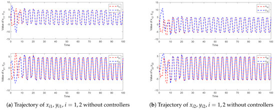
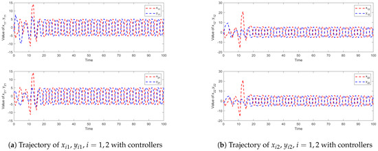
The state variables $x_{ij}$ and $y_{ij}$, $i,j=1,2$ of the drive system (2) and response system (4) are shown in Figure 1 without control inputs, clearly demonstrating the failure to achieve anti-synchronization between the nodes. Therefore, to achieve anti-synchronization of the nodes, the parameters for the controllers $u_i$, $i=1,2$ are selected as follows:

$$u_i\left(k\right)=\sum _{\varsigma =1}^2{\psi }_{\varsigma }\left(v\left(k\right)\right)[K_i^{\varsigma }{e}_i\left(k_s^i\right)-{\displaystyle \frac{Q_i\mathrm{sgn}\left({\mathrm{e}}_{\mathrm{i}}\left({\mathrm{k}}_{\mathrm{s}}^{\mathrm{i}}\right)\right)}{\parallel e\left(k_s^i\right)\parallel }}],$$

where

$${\psi }_1\left(v\left(k\right)\right)={\displaystyle \frac{{\sin }^2(\parallel \mathrm{e}\left(\mathrm{k}\right)\parallel )}{2}},{\psi }_2\left(v\left(k\right)\right)={\displaystyle \frac{1-{\sin }^2(\parallel \mathrm{e}\left(\mathrm{k}\right)\parallel )}{2}}.$$

The control gain matrix K and Q can be calculated as follows:

$$K_1^1=\left(\begin{array}{cc}-0.88& -0.65\\ -1.03& -1.34\end{array}\right),K_2^1=\left(\begin{array}{cc}-0.84& -0.67\\ -1.11& -1.35\end{array}\right),$$

$$K_1^2=\left(\begin{array}{cc}-0.77& -0.72\\ -1.02& -1.18\end{array}\right),K_2^2=\left(\begin{array}{cc}-0.82& -0.75\\ -1.15& -1.31\end{array}\right),$$

$$Q_1=\left(\begin{array}{cc}2.68& 2.67\\ 2.34& 2.11\end{array}\right),Q_2=\left(\begin{array}{cc}2.42& 2.98\\ 2.11& 2.13\end{array}\right).$$

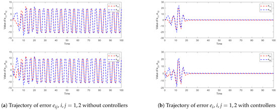
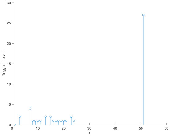
Other parameters include $\varrho =0.2$. Figure 2 show the simulation trajectories of the system state variables $x_{i1}$, $y_{i1}$ and $x_{2i}$, $y_{2i}$ reach anti-synchronization with each other under the controllers. Figure 3 shows the trajectory of the system error over 100 s, from which it can be clearly seen that the error converges to zero around 30 s. It is clear that the system is anti-synchronised by the controller (10). In addition, Figure 4 shows the trajectory of ETM. The values on the y-axis represent the time intervals between the current triggering instant and the previous one, from which it can be clearly observed that the system does not exhibit Zeno behavior.

5. Conclusions

To more accurately model practical memristor-based neural networks, this paper introduces a topological coupling structure and time-varying delays, developing a novel T-S fuzzy FMDTNNs model for the first time. An innovative ETM mechanism is then designed to investigate the anti-synchronization problem of this model. The proposed scheme integrates ETM with T-S fuzzy logic, mitigating nonlinearity effects while preventing unnecessary channel resource waste. Theoretical criteria to ensure the anti-synchronization of the system are then obtained through the Lyapunov direct method. It should be emphasized that the control parameters in this paper have not yet been optimized, and future research will focus on optimizing these parameters using the PSO algorithm.

References

- Snider, G. Cortical computing with memristive nanodevices. SciDAC Rev. 2008, 10, 58–65. [Google Scholar]
- Jo, S.H.; Chang, T.; Ebong, I.; Bhadviya, B.B.; Mazumder, P.; Lu, W. Nanoscale memristor device as synapse in neuromorphic systems. Nano Lett. 2010, 10, 1297–1301. [Google Scholar] [CrossRef]
- Kumar, D.; Li, H.; Kumbhar, D.D.; Rajbhar, M.K.; Das, U.K.; Syed, A.M.; Melinte, G.; El-Atab, N. Highly efficient back-end-of-line compatible flexible Si-based optical memristive crossbar array for edge neuromorphic physiological signal processing and bionic machine vision. Nano-Micro Lett. 2024, 16, 238. [Google Scholar] [CrossRef]
- Mou, X.; Tang, J.; Lyu, Y.; Zhang, Q.; Yang, S.; Xu, F.; Liu, W.; Xv, M.; Zhou, Y.; Sun, W.; et al. Analog memristive synapse based on topotactic phase transition for high-performance neuromorphic computing and neural network pruning. Sci. Adv. 2021, 7, eabh0648. [Google Scholar] [CrossRef] [PubMed]
- Shekinah Archita, S.; Ravi, V. A hybrid CMOS-memristor based adaptable bidirectional associative memory neural network for pattern recognition applications. Phys. Scr. 2025, 100, 035011. [Google Scholar]
- Huang, Y.; Li, A. General decay anti-synchronization of coupled delayed memristive neural networks with constant and time-varying distributed-delay coupling. Neurocomputing 2025, 618, 129058. [Google Scholar] [CrossRef]
- Cao, Y.; Jiang, W.; Wang, J. Anti-synchronization of delayed memristive neural networks with leakage term and reaction–diffusion terms. Knowl.-Based Syst. 2021, 233, 107539. [Google Scholar] [CrossRef]
- Li, H.; Hu, X.; Wang, Q.; Wang, L. Anti-synchronisation in fixed-/preassigned-time of delayed memristive neural networks with discontinuous activation functions. Int. J. Control 2024, 97, 2140–2150. [Google Scholar] [CrossRef]
- Murthy, G.R. Toward optimal synthesis of discrete-time Hopfield neural network. IEEE Trans. Neural Netw. Learn. Syst. 2022, 34, 9549–9554. [Google Scholar] [CrossRef]
- Ding, S.; Wang, Z.; Rong, N. Intermittent control for quasi-synchronization of delayed discrete-time neural networks. IEEE Trans. Cybern. 2020, 51, 862–873. [Google Scholar] [CrossRef]
- Priyanka, K.S.R.; Nagamani, G. Exponential H∞ synchronization and anti-synchronization of delayed discrete-time complex-valued neural networks with uncertainties. Math. Comput. Simul. 2023, 207, 301–321. [Google Scholar] [CrossRef]
- Zhang, T.; Yang, Y.; Han, S. Exponential heterogeneous anti-synchronization of multi-variable discrete stochastic inertial neural networks with adaptive corrective parameter. Eng. Appl. Artif. Intell. 2025, 142, 109871. [Google Scholar] [CrossRef]
- Liu, F.; Meng, W.; Lu, R. Anti-synchronization of discrete-time fuzzy memristive neural networks via impulse sampled-data communication. IEEE Trans. Cybern. 2022, 53, 4122–4133. [Google Scholar] [CrossRef]
- Podlubny, I. Fractional Differential Equations: An Introduction to Fractional Derivatives, Fractional Differential Equations, to Methods of Their Solution and Some of Their Applications; Elsevier: Amsterdam, The Netherlands, 1998; Volume 198. [Google Scholar]
- Kilbas, A.; Srivastava, H.; Trujillo, J. Theory and Applications of Fractional Differential Equations; Elsevier: Amsterdam, The Netherlands, 2006; Volume 204. [Google Scholar]
- Li, R.; Cao, J.; Li, N. Stabilization control of quaternion-valued fractional-order discrete-time memristive neural networks. Neurocomputing 2023, 542, 126255. [Google Scholar] [CrossRef]
- Li, H.L.; Cao, J.; Hu, C.; Jiang, H.; Alsaadi, F.E. Synchronization analysis of discrete-time fractional-order quaternion-valued uncertain neural networks. IEEE Trans. Neural Netw. Learn. Syst. 2024, 35, 14178–14189. [Google Scholar] [CrossRef]
- Perumal, R.; Hymavathi, M.; Ali, M.S.; Mahmoud, B.A.; Osman, W.M.; Ibrahim, T.F. Synchronization of discrete-time fractional-order complex-valued neural networks with distributed delays. Fractal Fract. 2023, 7, 452. [Google Scholar] [CrossRef]
- Yang, J.; Li, H.L.; Zhang, L.; Hu, C.; Jiang, H. Synchronization of discrete-time fractional fuzzy neural networks with delays via quantized control. ISA Trans. 2023, 141, 241–250. [Google Scholar] [CrossRef]
- Cui, X.; Li, H.L.; Zhang, L.; Hu, C.; Bao, H. Complete synchronization for discrete-time fractional-order coupled neural networks with time delays. Chaos Solitons Fractals 2023, 174, 113772. [Google Scholar] [CrossRef]
- Zhang, X.L.; Li, H.L.; Yu, Y.; Zhang, L.; Jiang, H. Quasi-projective and complete synchronization of discrete-time fractional-order delayed neural networks. Neural Netw. 2023, 164, 497–507. [Google Scholar] [CrossRef]
- Ping, J.; Zhu, S.; Liu, X. Finite/fixed-time synchronization of memristive neural networks via event-triggered control. Knowl.-Based Syst. 2022, 258, 110013. [Google Scholar] [CrossRef]
- Wu, J.; Yu, Y.; Ren, G. Leader-following formation control for discrete-time fractional stochastic multi-agent systems by event-triggered strategy. Fractal Fract. 2024, 8, 246. [Google Scholar] [CrossRef]
- Lu, Y.; Wu, X.; Wang, Y.; Huang, L.; Wei, Q. Quantization-based event-triggered H∞ consensus for discrete-time Markov jump fractional-order multiagent systems with DoS attacks. Fractal Fract. 2024, 8, 147. [Google Scholar] [CrossRef]
- Priyanka, K.S.R.; Soundararajan, G.; Kashkynbayev, A.; Nagamani, G. Co-existence of robust output-feedback synchronization and anti-synchronization of delayed discrete-time neural networks with its application. Comput. Appl. Math. 2024, 43, 77. [Google Scholar] [CrossRef]
- Pratap, A.; Raja, R.; Cao, J.; Huang, C.; Niezabitowski, M.; Bagdasar, O. Stability of discrete-time fractional-order time-delayed neural networks in complex field. Math. Methods Appl. Sci. 2021, 44, 419–440. [Google Scholar] [CrossRef]
- Abdeljawad, T.; Atici, F.M. On the definitions of nabla fractional operators. Abstr. Appl. Anal. 2012, 2012, 406757. [Google Scholar] [CrossRef]
- Abdeljawad, T.; Baleanu, D. Discrete fractional differences with nonsingular discrete Mittag-Leffler kernels. Adv. Differ. Equ. 2016, 2016, 232. [Google Scholar] [CrossRef]
Disclaimer/Publisher’s Note: The statements, opinions and data contained in all publications are solely those of the individual author(s) and contributor(s) and not of MDPI and/or the editor(s). MDPI and/or the editor(s) disclaim responsibility for any injury to people or property resulting from any ideas, methods, instructions or products referred to in the content. |
© 2025 by the authors. Licensee MDPI, Basel, Switzerland. This article is an open access article distributed under the terms and conditions of the Creative Commons Attribution (CC BY) license (https://creativecommons.org/licenses/by/4.0/).