

Application of Mathematical Modeling and Numerical Simulation of Blood Biomarker Transport in Paper-Based Microdevices


Abstract
1. Introduction
2. Mathematical Model
2.1. Mathematical Model for Fluid Flow in Paper Strips and Microdevices
2.2. Mathematical Model for the Temperature in the Paper Strip Used for Microdevices
2.3. Mathematical Model for Solute Transport in the Paper Strip Used for Microdevices
3. Studied Cases: Geometry, Materials, and Initial and Boundary Conditions
3.1. Two-Dimensional Simulation (2D)
Initial and Boundary Conditions
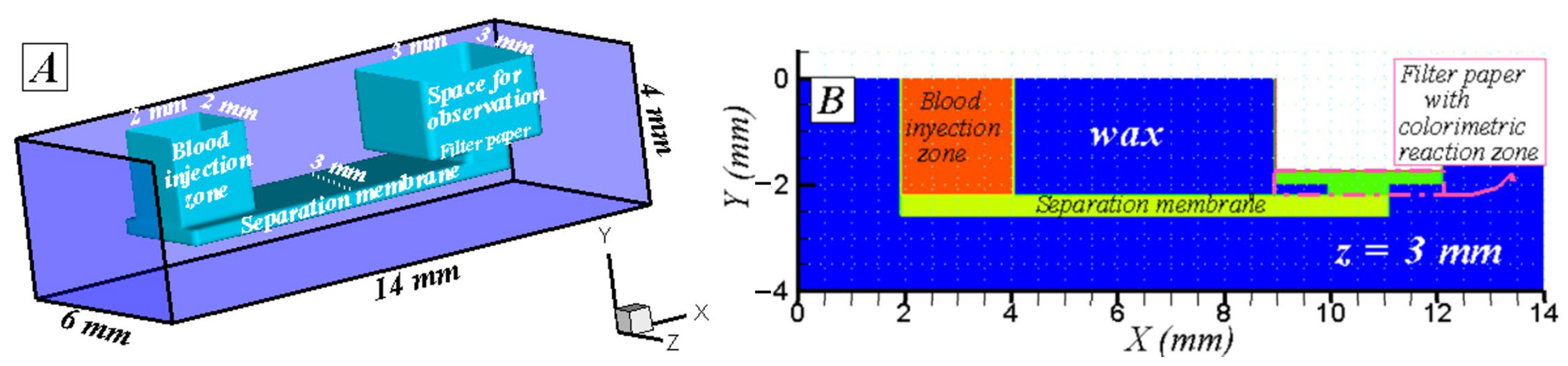
3.2. Three-Dimensional Simulation (3D)
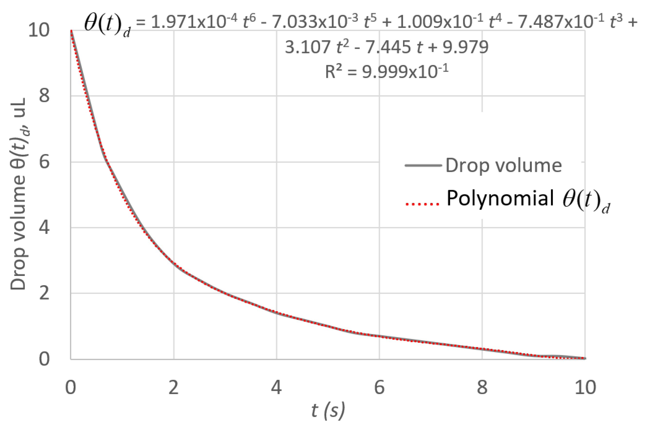
Initial and Boundary Conditions
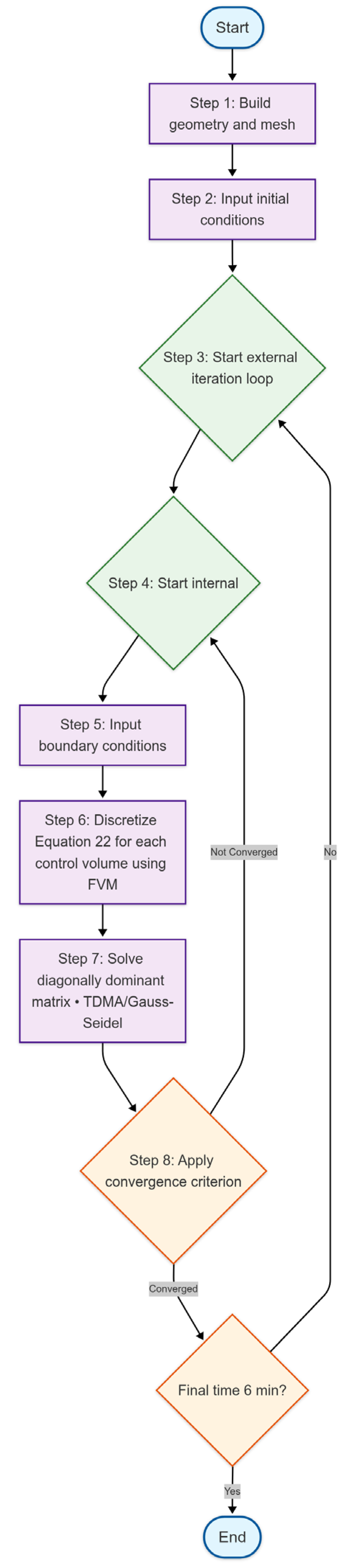
4. Computational Procedure
5. Results
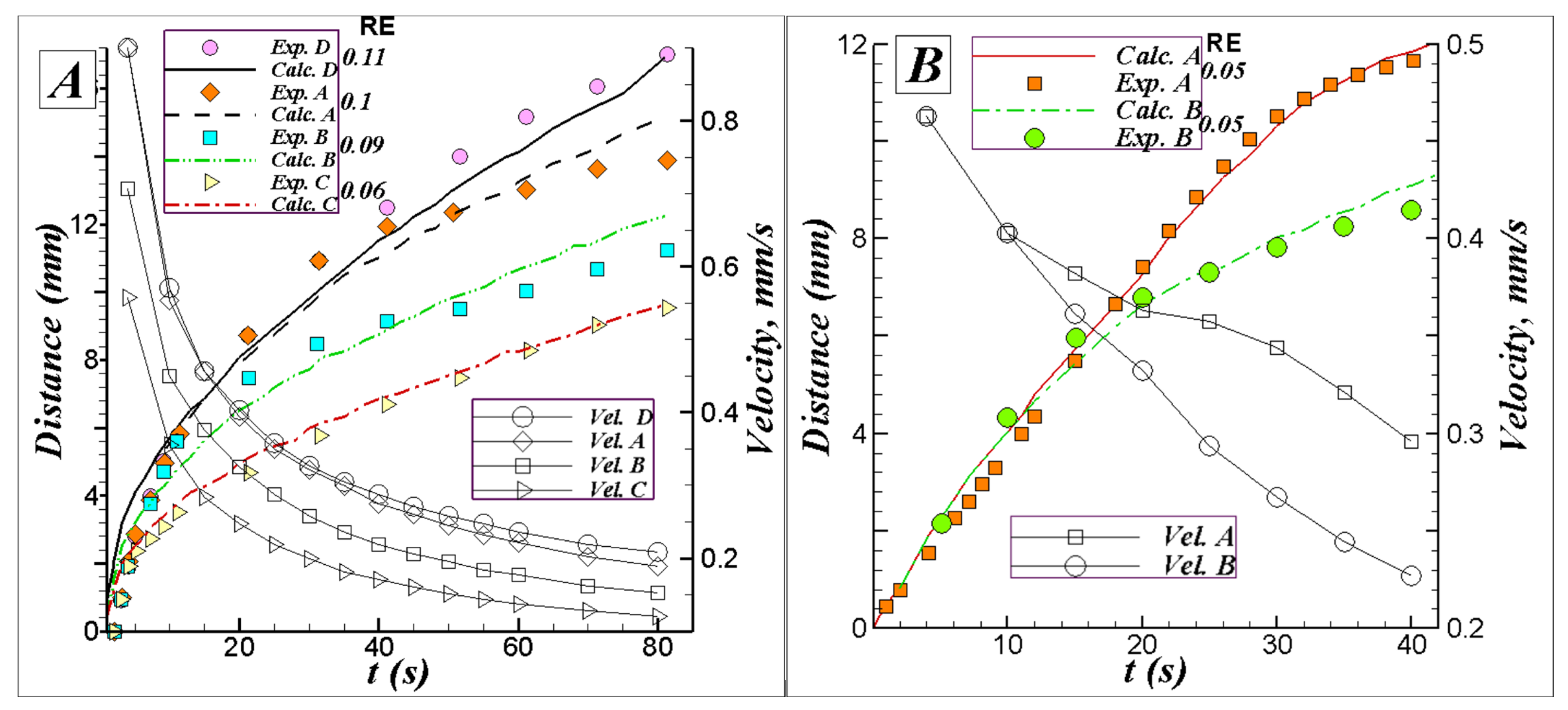
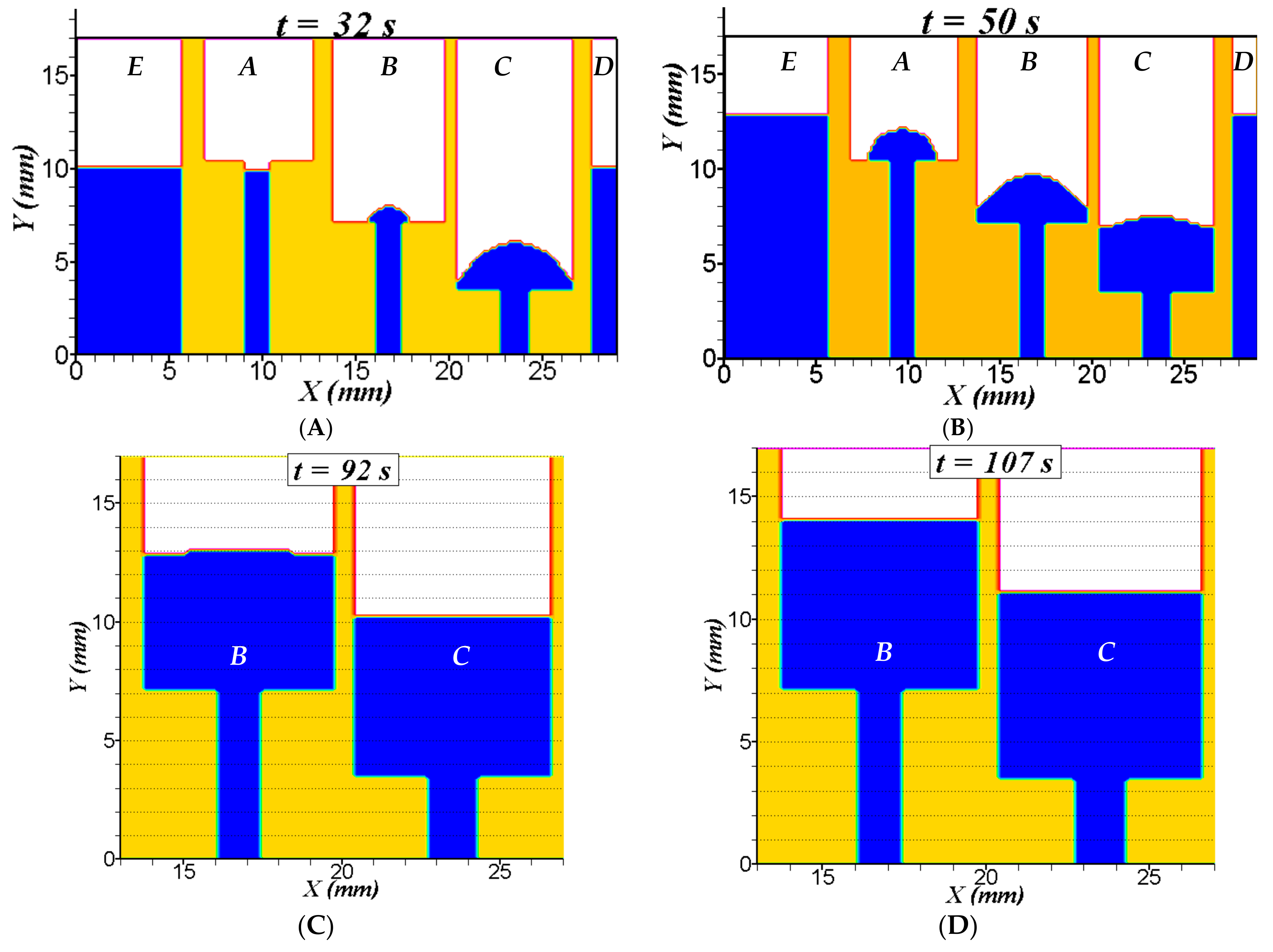
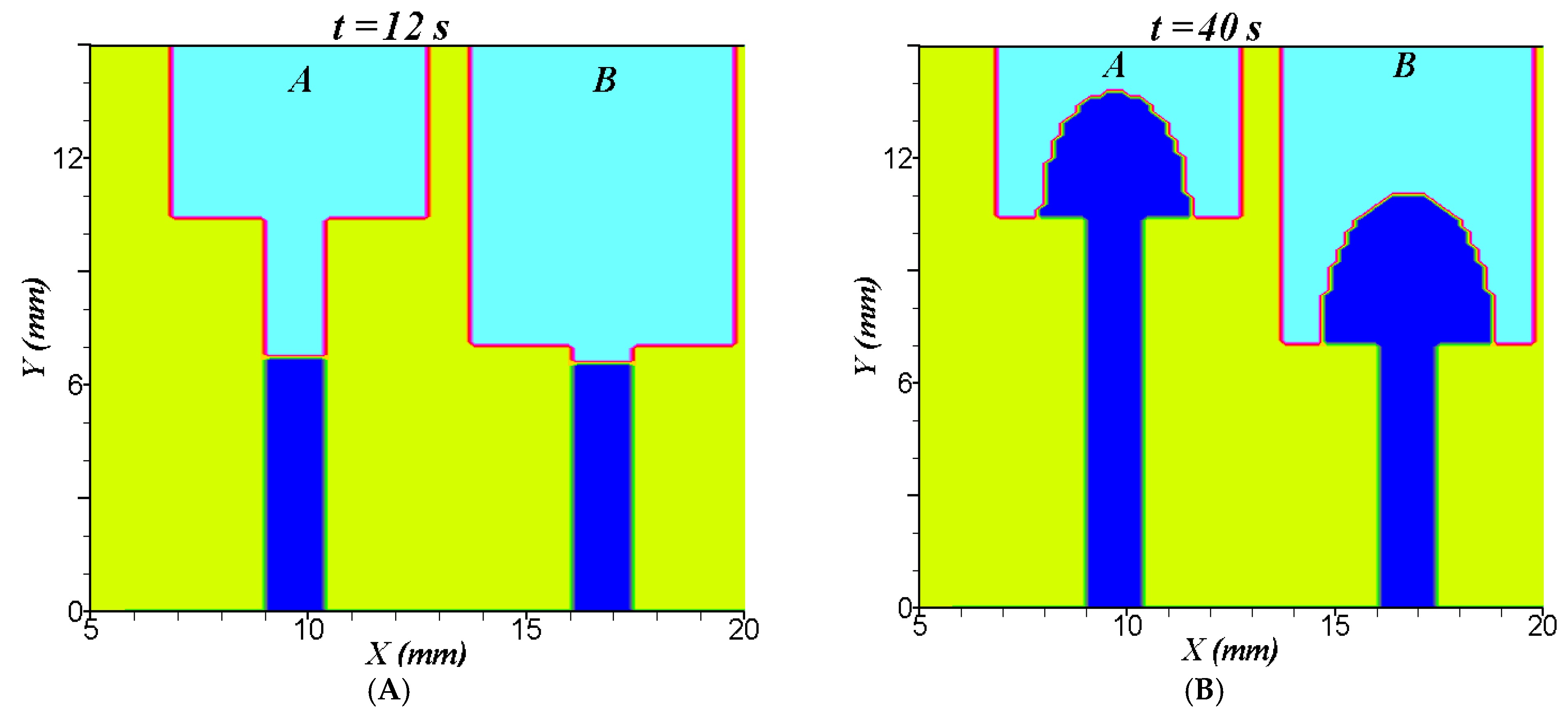
5.1. Results for Two-Dimensional Diffusion of Water and Solute in Strips with Variable Widths
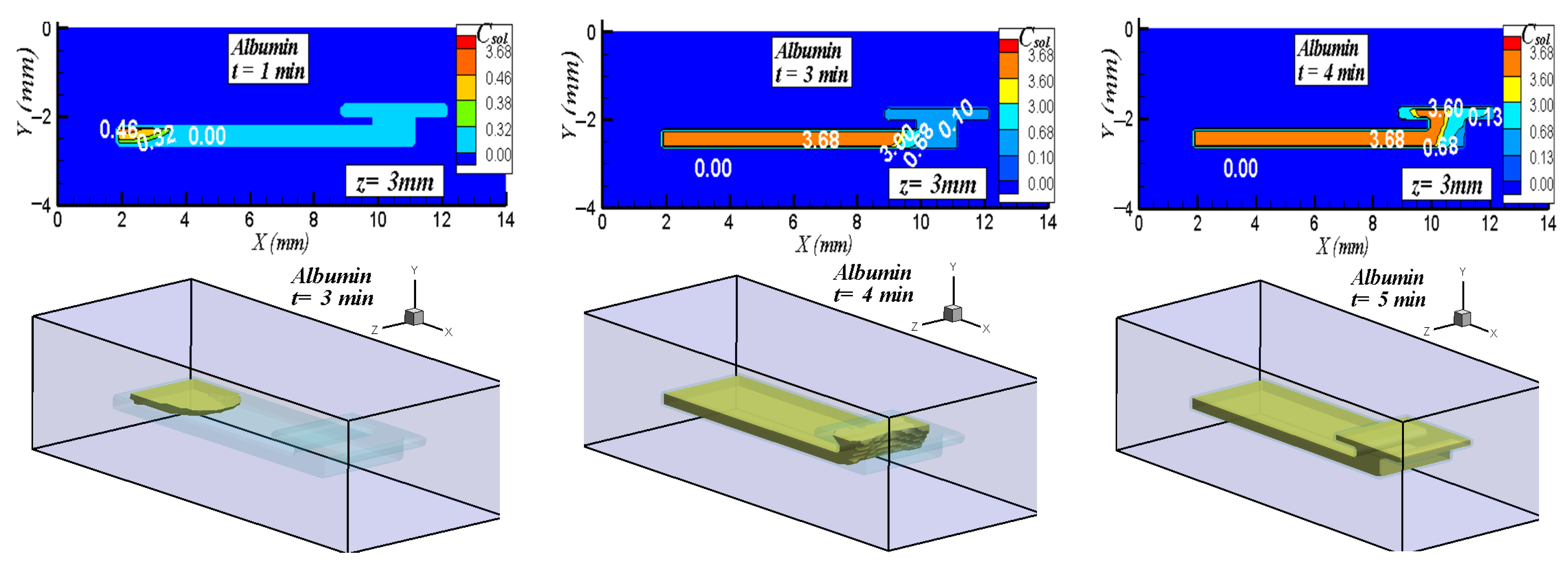
5.2. Three-Dimensional Simulation of Blood Transport in a Paper-Based Microdevice Used to Detect Albumin
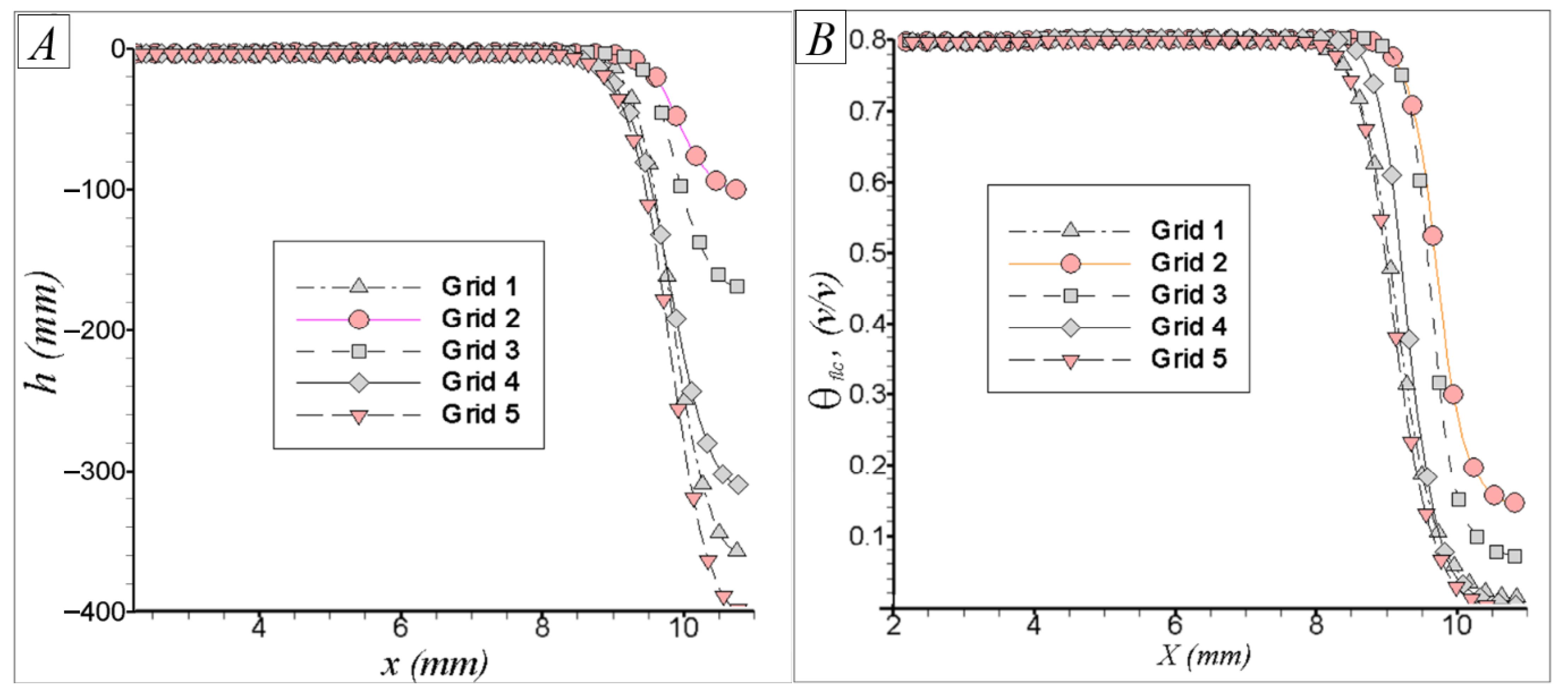
5.2.1. Mesh Analysis
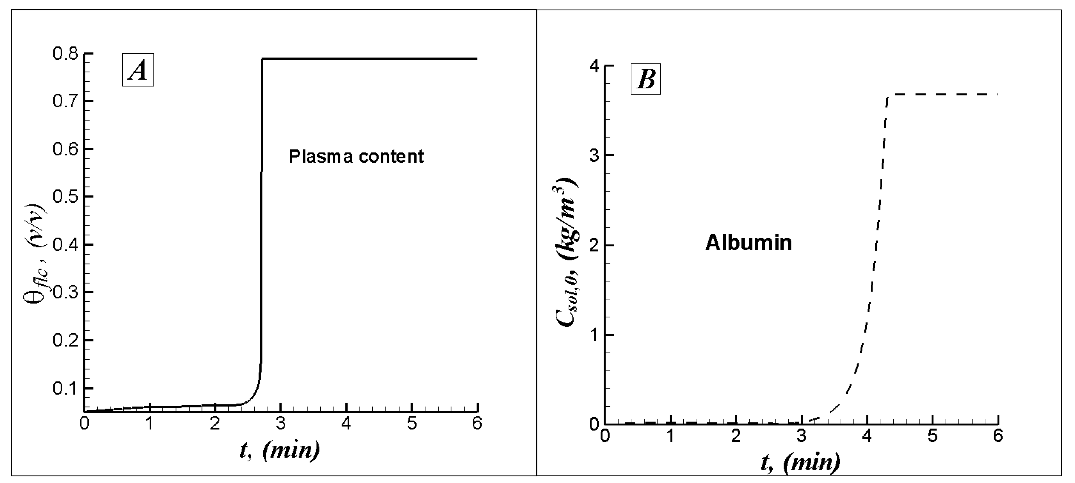
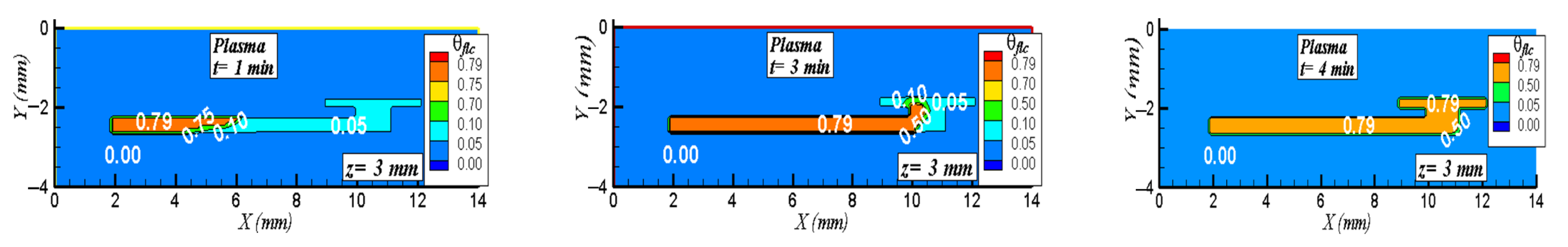
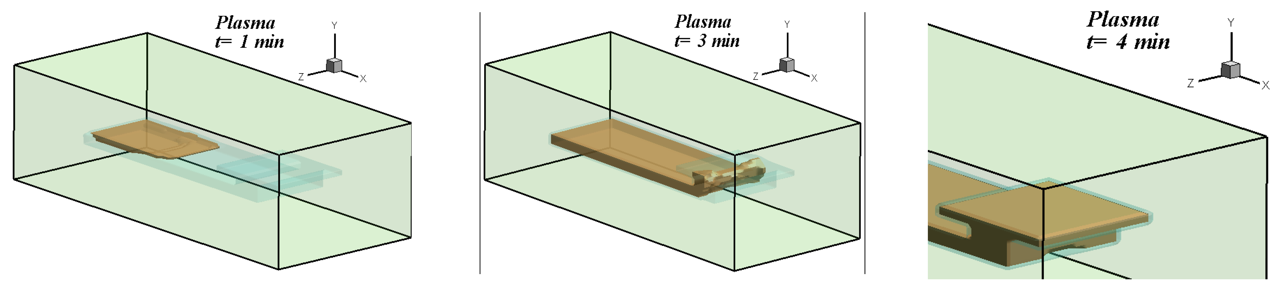
5.2.2. Results and Analysis for the 3D Case
6. Conclusions
Supplementary Materials
Author Contributions
Funding
Data Availability Statement
Conflicts of Interest
References
- Gao, D.; Ma, Z.; Jiang, Y. Recent Advances in Microfluidic Devices for Foodborne Pathogens Detection. TrAC-Trends Anal. Chem. 2022, 157, 116788. [Google Scholar] [CrossRef]
- Espinosa, A.; Diaz, J.; Vazquez, E.; Acosta, L.; Santiago, A.; Cunci, L. Fabrication of Paper-Based Microfluidic Devices Using a 3D Printer and a Commercially-Available Wax Filament. Talanta Open 2022, 6, 100142. [Google Scholar] [CrossRef]
- Morbioli, G.G.; Mazzu-Nascimento, T.; Stockton, A.M.; Carrilho, E. Technical Aspects and Challenges of Colorimetric Detection with Microfluidic Paper-Based Analytical Devices (ΜPADs)—A Review. Anal. Chim. Acta 2017, 970, 1–22. [Google Scholar] [CrossRef] [PubMed]
- Narasimhan, A.; Jain, H.; Muniandy, K.; Chinnappan, R.; Mani, N.K. Bio-Analysis of Saliva Using Paper Devices and Colorimetric Assays. J. Anal. Test. 2023, 8, 114–132. [Google Scholar] [CrossRef]
- Patari, S.; Datta, P.; Mahapatra, P.S. 3D Paper-Based Milk Adulteration Detection Device. Sci. Rep. 2022, 12, 13657. [Google Scholar] [CrossRef]
- Yang, R.J.; Tseng, C.C.; Ju, W.J.; Fu, L.M.; Syu, M.P. Integrated Microfluidic Paper-Based System for Determination of Whole Blood Albumin. Sens. Actuators B Chem. 2018, 273, 1091–1097. [Google Scholar] [CrossRef]
- Lepowsky, E.; Ghaderinezhad, F.; Knowlton, S. Paper-Based Assays for Urine Analysis. Biomicrofluidics 2017, 11, 051501. [Google Scholar] [CrossRef]
- Torul, H.; Caglayan, Z.; Tezcan, T.; Calik, E.; Calimci, M.; Gumustas, A.; Yildirim, E.; Kulah, H.; Tamer, U. Microfluidic-Based Bood Inmunoassays. J. Pharm. Biomed. Anal. 2023, 228, 115313. [Google Scholar] [CrossRef] [PubMed]
- Mathew, J.; Sankar, P.; Varacallo, M. Physiology, Blood Plasma. NCBI Bookshelf. 2023. Available online: https://www.ncbi.nlm.nih.gov/books/NBK531504/ (accessed on 9 June 2025).
- Li, H.; Han, D.; Hegener, M.A.; Pauletti, G.M.; Steckl, A.J. Flow Reproducibility of Whole Blood and Other Bodily Fluids in Simplified No Reaction Lateral Flow Assay Devices. Biomicrofluidics 2017, 11, 024116. [Google Scholar] [CrossRef]
- Ranucci, M.; Laddomada, T.; Ranucci, M.; Baryshnikova, E. Blood Viscosity during Coagulation at Different Shear Rates. Physiol. Rep. 2014, 2, e12065. [Google Scholar] [CrossRef]
- Fu, E.; Ramsey, S.A.; Kauffman, P.; Lutz, B.; Yager, P. Transport in Two-Dimensional Paper Networks. Microfluid. Nanofluid. 2011, 10, 29–35. [Google Scholar] [CrossRef] [PubMed]
- Song, K.; Huang, R.; Hu, X. Imbibition of Newtonian Fluids in Paper-like Materials with the Infinitesimal Control Volume Method. Micromachines 2021, 12, 1391. [Google Scholar] [CrossRef] [PubMed]
- Li, L.; Huang, H.; Lin, X.M.; Fan, X.; Sun, Y.; Zhou, W.; Wang, T.; Bei, S.; Zheng, K.; Xu, Q.; et al. Enhancing the Performance of Paper-Based Microfluidic Fuel Cell via Optimization of Material Properties and Cell Structures: A Review. Energy Convers. Manag. 2024, 305, 9–11. [Google Scholar] [CrossRef]
- Jafari Ghahfarokhi, N.; Mosharaf-Dehkordi, M.; Bayareh, M. Experimental and Numerical Assessment and Performance Optimization of a Novel T-Arrow Microfluidic Device to Mix Two Fluids with Different Thermophysical Properties. Chem. Eng. Process.-Process Intensif. 2024, 201, 109808. [Google Scholar] [CrossRef]
- Wu, B.; Xu, X.; Dong, G.; Zhang, M.; Luo, S.; Leung, D.Y.C.; Wang, Y. Computational Modeling Studies on Microfluidic Fuel Cell: A Prospective Review. Renew. Sustain. Energy Rev. 2024, 191, 114082. [Google Scholar] [CrossRef]
- Papadopoulos, V.E.; Kefala, I.N.; Kaprou, G.D.; Tserepi, A.; Kokkoris, G. Modeling Heat Losses in Microfluidic Devices: The Case of Static Chamber Devices for DNA Amplification. Int. J. Heat Mass Transf. 2022, 184, 122011. [Google Scholar] [CrossRef]
- Abit, S.M.; Amoozegar, A.; Vepraskas, M.J.; Niewoehner, C.P. Solute Transport in the Capillary Fringe and Shallow Groundwater: Field Evaluation. Vadose Zone J. 2008, 7, 890–898. [Google Scholar] [CrossRef]
- Radcliffe, D.E.; Simunek, J. Soil Physics with Hydrus; CRC Press, Taylor & Francis: Boca Raton, FL, USA, 2010; ISBN 9781420073805. [Google Scholar]
- Serrano, S.E. Modeling Infiltration with Approximate Solutions to Richard’s Equation. J. Hydrol. Eng. 2004, 9, 421–432. [Google Scholar] [CrossRef]
- Jury, W.; Horton, R. Soil Physics, 6th ed.; John Wiley & Sons: Noida, India, 2013. [Google Scholar]
- Simunek, J.; Sejna, M.; Brunetti, G.; Van Genuchten, M. Hydrus 1D: Technical Manual I. Version 5.04, 5th ed.; Pc-Progress: Prague, Czech Republic, 2024. [Google Scholar]
- Chao, T.C.; Arjmandi-Tash, O.; Das, D.B.; Starov, V.M. Spreading of Blood Drops over Dry Porous Substrate: Complete Wetting Case. J. Colloid Interface Sci. 2015, 446, 218–225. [Google Scholar] [CrossRef]
- Patankar, S.V. Computational of Conduction and Duct Flow Heat Transfer; CRC: Boca Raton, FL, USA; Taylor & Francis Group: Abingdon, UK, 1991. [Google Scholar]
- Veersteg, H.M.; Malalasekera, W. An Introductionto Computational Fluid Dynamic: The Finite Volume Method, 2nd ed.; Hall, P., Ed.; Pearson: Harlow, UK, 2007. [Google Scholar]
- Merck Millipore. Rapid Lateral Flow Test Strips Considerations for Product Development; Merck Millipore: Darmstadt, Germany, 2018; Volume 33, Available online: https://www.merckmillipore.com/INTERSHOP/web/WFS/Merck-RU-Site/ru_RU/-/USD/ShowDocument-Pronet?id=201306.15671 (accessed on 6 June 2025).
- Costa, A. Permeability-porosity Relationship: A Reexamination of the Kozeny-Carman Equation Based on a Fractal Pore-Space Geometry Assumption. Geophys. Res. Lett. 2006, 33, L02318. [Google Scholar] [CrossRef]
- Ashkezari, A.Z.; Jolfaei, N.A.; Jolfaei, N.A.; Hekmatifar, M.; Toghraie, D.; Sabetvand, R.; Rostami, S. Calculation of the Thermal Conductivity of Human Serum Albumin (HSA) with Equilibrium/Non-Equilibrium Molecular Dynamics Approaches. Comput. Methods Programs Biomed. 2020, 188, 105256. [Google Scholar] [CrossRef] [PubMed]
- Bharadwaj Reddy, P.; Gunasekar, C.; Mhaske, A.S.; Vijay Krishna, N. Enhancement of Thermal Conductivity of PCM Using Filler Graphite Powder Materials. In Proceedings of the 2nd International Conference on Advances in Mechanical Engineering (Icame2028), Kattankulathur, India, 22–24 March 2018, IOP Conference Series: Materials Science and Engineering; IOP Publishing: Bristol, UK, 2018; Volume 402. [Google Scholar]
- Xu, F.; Lu, T.J.; Seffen, K.A.; Ng, E.Y.K. Mathematical Modeling of Skin Bioheat Transfer. Appl. Mech. Rev. 2009, 62, 050801. [Google Scholar] [CrossRef]
- PALL LIFE Sciences. Membrane Asymmetric Polysulfone Vivid TM Plasma Separation Membrane. 2009. Available online: https://shop.pall.com/us/en/attachment?LocaleId=en_US&DirectoryPath=pdfs%2FOEM-Materials-and-Devices&FileName=09.2730_VividPlasma_DS_6pg.pdf&UnitName=PALL (accessed on 6 June 2025).
- Nalumachu, R.; Anandita, A.; Rath, D. Computational Modelling of a Competitive Immunoassay in Lateral Flow Diagnostic Devices. Sens. Diagn. 2023, 2, 687–698. [Google Scholar] [CrossRef]
- Millington, R.J.; Quirk, J.P. Permeability of Porous Solids. Trans. Faraday Soc. 1961, 57, 1200–1207. [Google Scholar] [CrossRef]


| (N/m) ** | (m) * | (kg/s m) ** | (m2/s) | ϑ2 | λ | αff |
| 0.072 | 1.16 × 10⁻⁵ | 0.001 | 2.088 × 10⁻⁴ | 2.093 × 10⁻⁴ | 6 × 10⁻⁶ | 0.8 |
| Dsol,x (m2/s) | Dsol,y (m2/s) | Jw,in+ (m/s) | Jsol,in (m/s) | |||
| 2 × 10⁻⁸ | 1 × 10⁻⁷ | 2.963 × 10⁻⁴ | 5 × 10⁻³ | 0 |
| Paper Strip | A | B | C | D |
|---|---|---|---|---|
| , mm2 | 39 | 59 | 79 | 20 |
| mm/s | 0.35 | 0.28 | 0.22 | 0.36 |
| mm/s | 0.19 | 0.15 | 0.12 | 0.19 |
| mm/s | 0.37 | 0.32 | - | - |
| mm/s | 0.05 | 0.08 | - | - |
| , mm | , m−1 | , m2 | , mm | ||||
|---|---|---|---|---|---|---|---|
| Strip B–C | 3.5 | 0.785 | 6.5 | 8330 | 3.86 × 10⁻⁸ | 3.15 × 10⁻³ | 6.7 |
| (kg/m3) ++ | (J/kg°C) ++ | (W/m K) ++ | (J/m3K) + | (kg/m3) + | ||
| 0.051 | 0.8 | 1025 | 3930 | 0.525 | 1850 | 856 |
(W/m K) + | %albumin in blood * | (kg/m3) ** | (J/kg °C) ** | (W/m K) ** | xx | xx |
| 0.4 | 3 | 3560 | 1100 | 0.496 | 5 | −1 |
| (cm2/h) xxx | (cm) a | (cm) a | (cm) a | (kg/m3) *** | (1/cm) | |
| 0.0416 | 100 | 30 | 30 | 3.68 | 0.05 | 0.8 |
| N° Mesh | N° of CVs in x,y,z | Total N° of CVs | N° CVs in Separation and Filter Paper Zone | %RE |
|---|---|---|---|---|
| 1 | 188 × 42 × 68 | 536,928 | 119,070 | 0 |
| 2 | 148 × 28 × 53 | 219,632 | 43,747 | 9.9 |
| 3 | 158 × 33 × 53 | 276,342 | 54,612 | 7.8 |
| 4 | 168 × 33 × 53 | 293,832 | 58,220 | 2.0 |
| 5 | 196 × 38 × 58 | 431,984 | 93,420 | 0.81 |
Disclaimer/Publisher’s Note: The statements, opinions and data contained in all publications are solely those of the individual author(s) and contributor(s) and not of MDPI and/or the editor(s). MDPI and/or the editor(s) disclaim responsibility for any injury to people or property resulting from any ideas, methods, instructions or products referred to in the content. |
© 2025 by the authors. Licensee MDPI, Basel, Switzerland. This article is an open access article distributed under the terms and conditions of the Creative Commons Attribution (CC BY) license (https://creativecommons.org/licenses/by/4.0/).
Share and Cite
Zambra, C.E.; Hernandez, D.; Morales-Ferreiro, J.O.; Vasco, D. Application of Mathematical Modeling and Numerical Simulation of Blood Biomarker Transport in Paper-Based Microdevices. Mathematics 2025, 13, 1936. https://doi.org/10.3390/math13121936
Zambra CE, Hernandez D, Morales-Ferreiro JO, Vasco D. Application of Mathematical Modeling and Numerical Simulation of Blood Biomarker Transport in Paper-Based Microdevices. Mathematics. 2025; 13(12):1936. https://doi.org/10.3390/math13121936
Chicago/Turabian StyleZambra, Carlos E., Diógenes Hernandez, Jorge O. Morales-Ferreiro, and Diego Vasco. 2025. "Application of Mathematical Modeling and Numerical Simulation of Blood Biomarker Transport in Paper-Based Microdevices" Mathematics 13, no. 12: 1936. https://doi.org/10.3390/math13121936
APA StyleZambra, C. E., Hernandez, D., Morales-Ferreiro, J. O., & Vasco, D. (2025). Application of Mathematical Modeling and Numerical Simulation of Blood Biomarker Transport in Paper-Based Microdevices. Mathematics, 13(12), 1936. https://doi.org/10.3390/math13121936