Alzheimer’s Disease Detection in Various Brain Anatomies Based on Optimized Vision Transformer

Abstract

Alzheimer’s disease (AD) is a progressive neurodegenerative disorder and a growing public health concern. Despite significant advances in deep learning for medical image analysis, early and accurate diagnosis of AD remains challenging. In this study, we focused on optimizing the training process of deep learning models by proposing an enhanced version of the Adam optimizer. The proposed optimizer introduces adaptive learning rate scaling, momentum correction, and decay modulation to improve convergence speed, training stability, and classification accuracy. We integrated the enhanced optimizer with Vision Transformer (ViT) and Convolutional Neural Network (CNN) architectures. The ViT-based model comprises a linear projection of image patches, positional encoding, a transformer encoder, and a Multi-Layer Perceptron (MLP) head with a Softmax classifier for multiclass AD classification. Experiments on publicly available Alzheimer’s disease datasets (ADNI-1 and ADNI-2) showed that the enhanced optimizer enabled the ViT model to achieve a 99.84% classification accuracy on Dataset-1 and 95.75% on Dataset-2, outperforming Adam, RMSProp, and SGD. Moreover, the optimizer reduced entropy loss and improved convergence stability by 0.8–2.1% across various architectures, including ResNet, RegNet, and MobileNet. This work contributes a robust optimizer-centric framework that enhances training efficiency and diagnostic accuracy for automated Alzheimer’s disease detection.

1. Introduction

In recent years, Alzheimer’s disease (AD) has emerged as a serious threat to human health. The World Health Organization (WHO) warned about rapidly increasing Alzheimer’s disease and provided statistics on its official website [1]. According to WHO, approximately 55 million people have dementia around the globe. The figures are expected to increase up to 78 million by 2030. Around 70% of the patients with dementia have Alzheimer’s disease. This raises a serious health concern for people around the world. AD is a progressive degenerative disease, where abnormal build-up of amyloid and tau proteins in the brain lead to progressive cell death, causing a decline in memory functions and cognitive impairment.

Researchers have proposed many data-driven models, among which Convolutional Neural Networks (CNNs) are the most widely used [2]. CNNs have been widely applied in medical image analysis, including the detection of brain tumors, Alzheimer’s disease, Parkinson’s disease, and various types of cancer. Recently, CNNs have been increasingly applied to brain images in diagnostic and prognostic tasks, which enables the learning of many robust features. Vision Transformer (ViT), originally developed for natural language processing, has recently gained attention in computer vision as an effective alternative to CNNs. Transformers have been used for natural language processing tasks, but their application to image processing remains limited.

Optimizers play a vital role in improving the training efficiency and generalization of deep learning models [3]. Various optimization algorithms have been proposed over the years, each with specific trade-offs affecting convergence speed, accuracy, and memory efficiency. However, common limitations are still present in existing optimizers, including the following:

• Slow convergence on large datasets due to full-batch updates.
• Risk of being trapped in local minima.
• High memory requirements for gradient computation.

To address these challenges, we propose an enhanced version of the Adam optimizer that incorporates adaptive learning rate scaling, momentum correction, and decay modulation. Our method aims to improve training stability, reduce entropy loss, and achieve faster convergence without increasing computational complexity. Unlike the traditional Adam, which statically adjusts moment estimates and learning rates, our optimizer introduces a dynamic scaling factor and simplified update strategy to mitigate instability and overfitting. Our contribution is summarized in the following list:

• We develop an enhanced optimizer that integrates adaptive learning rate scaling and momentum modulation, built upon established principles. Our method dynamically adjusts the step size using second-moment estimates, ensuring stable and efficient weight updates while mitigating aggressive fluctuations.
• We introduce a novel combination of momentum correction and decay modulation strategies, which refine the optimization process by reducing oscillations, improving convergence consistency, and enhancing generalization across diverse deep learning architectures.
• We comprehensively evaluate the optimizer across multiple models, including ViT, ResNet, RegNet, and MobileNet, using publicly available Alzheimer’s disease datasets. The results demonstrate consistent improvements in training stability, convergence behavior, and classification accuracy compared to widely used optimizers such as Adam, RMSProp, and SGD.

The remaining part of this paper is organized as follows. In Section 2, the literature review is briefly presented. In Section 2, different optimization algorithms and the popular architecture-based machine learning models are explained in detail. Section 3 includes the proposed methodology. In Section 3, the experimental environment and datasets are described. Section 4 justifies the results through comparisons provided in the form of visual and statistical observations. In Section 5, we discuss the important aspects, limitations, and future work of this research. Section 6 concludes the study.

2. Literature Review

This section is organized in two parts: optimization algorithms and machine learning models [4].

2.1. Optimization Algorithms

Optimization is a very important part of the neural network training [5]. Its goal is to find the best set of weights/parameters that would yield a better performance specifically for the provided problem. Different methods are used for finding the optimal solution in machine learning’s training process. Each method holds its advantages and disadvantages, which may or may not affect the training process, depending on the hyper-parameter configurations as well. The most popular optimization technique is gradient descent, which is used in neural networks and repeatedly involves the value adjustment of the network parameters until the performance improves. Each type of problem is optimized using different methods. This refers to the fact that all problems cannot be solved using the gradient descent approach, which may necessitate the use of another type of optimization technique [6].

Training the neural network model involves the setup of the best understood parameters that are used to train the model and learn patterns over the provided data. Based on the type of model, the network learns patterns from the data and performs the desired task. To train a network, the loss function plays a very important role in validating and evaluating the neural network model’s performance. This function, while training, evaluates the output of the current network model and associates a numerical value to it to better represent the performance. These parametric values must be set in such a way that the network is able to perform the task well enough by minimizing the provided loss function value. Minimizing these values is performed iteratively by adjusting the network’s parametric values, and this procedure is known as training.

2.1.1. SGD

Neural networks are trained using various methods, each with its own benefits. The most common is gradient descent [7], where weight values are iteratively adjusted to minimize the loss function until optimal performance is achieved.

Gradient descent methods [8] are widely adopted due to their ease of implementation, high accuracy, and efficiency, even on large networks. They are stable and allow for tradeoffs between speed and stability. However, they may require many iterations and become computationally expensive on complex datasets, especially as all training samples are used to calculate derivatives, making it unsuitable for large data.

Stochastic Gradient Descent (SGD) [9] addresses this by updating weights using subsets of data, making it more scalable. The process involves initializing parameters and iteratively updating gradients based on the loss function. Despite its stability, SGD may be inefficient for complex datasets and slows down when gradients become small.

To mitigate this, momentum-based methods accelerate training by taking larger steps and avoiding small gradients. Nesterov Accelerated Gradient further improves this by using anticipated gradients. These techniques improve training performance but are still limited by incremental optimization steps.

SGD remains widely used in deep learning due to its scalability and availability. Its formulation is shown in Equation  (1):

$$\begin{array}{c}W=\omega -\eta \nabla Q_i\left(\omega \right)\\ W\leftarrow \eta \nabla Q\left(\omega \right)\\ Q\left(\omega \right)=ln{\displaystyle \sum _i}{Q}_i\left(\omega \right)\Rightarrow \nabla Q\left(\omega \right)=ln{\displaystyle \sum _i}\nabla Q_i\left(\omega \right)\end{array}$$

(1)

Here, $\omega$ is the initial weight, $\eta$ the learning rate, and $Q_i$ the data sample loss. Q denotes the overall error function. SGD minimizes Q by computing gradients and updating weights W accordingly.

2.1.2. RMSProp

RMSProp [10] is a technique used to reduce noise in neural networks by employing root mean squared propagation. It smooths errors across the network and improves performance, especially in deep architectures.

To reduce model error, two main approaches are used: regularization to penalize large weights and weight decay [11] to smooth values passed between layers. Finding the right level of regularization is difficult, especially in deep networks. RMSProp simplifies training by avoiding explicit regularization and using a more straightforward mechanism [12].

RMSProp was proposed by Hinton as an extension of gradient descent and AdaGrad, using a decaying average of squared gradients [13]. It adapts the step size for each parameter individually. The update rule is given in Equation (2):

$$\begin{array}{c}{v}_t=\delta \ast v_{t-1}-(1-\delta )\ast g_t^2\\ \Delta {\omega }_t=-{\displaystyle \frac{\eta }{\sqrt{y_t+ϵ}}}\ast g_t\\ {\omega }_{t+1}={\omega }_t+\Delta {\omega }_t\end{array}$$

(2)

In Equation (2), $\eta$ is the learning rate, $v_t$ is the running average of squared gradients, and $g_t$ is the gradient at time t. RMSProp effectively adjusts weights during training, improving generalization and reducing overfitting.

2.1.3. Adagrad

Adagrad is a short form of the Adaptive Gradient Algorithm; it is an optimization method that adapts the learning rate for each parameter individually. This is useful in cases involving sparse data, such as natural language processing or recommendation systems. In Adagrad, parameters with frequent updates are assigned smaller learning rates, while infrequent parameters receive larger updates, enabling more balanced learning [14].

Let $g_t$ denote the gradient of the loss with respect to the parameter $\theta$ at time step t. Adagrad maintains a cumulative sum of the squares of past gradients for each parameter, denoted as $G_t={\sum }_{i=1}^t{g}_i^2$, where the square and sum operations are performed element-wise. To ensure numerical stability and avoid division by zero, a small constant $ϵ$ is added. The update rule for Adagrad is given in Equation (3).

$${\theta }_{t+1}={\theta }_t-{\displaystyle \frac{\eta }{\sqrt{G_t+ϵ}}}·g_t$$

(3)

In Equation (3), $\eta$ is the initial learning rate, and the division is element-wise. As training progresses, $G_t$ accumulates, effectively reducing the learning rate for parameters with large gradients. However, one limitation of Adagrad is that $G_t$ can grow very large over time, causing the learning rate to shrink excessively and halt learning prematurely.

2.1.4. AdaDelta

AdaDelta is an improvement over the Adagrad optimizer that addresses its main drawback—rapid and unbounded decay of learning rates. Instead of accumulating all past squared gradients, AdaDelta uses an exponentially decaying average of the squared gradients, allowing the algorithm to continue learning throughout training. Moreover, AdaDelta dynamically adapts the learning rate by also maintaining a moving average of squared parameter updates, eliminating the need to manually set a global learning rate [15].

Let $E{\left[g^2\right]}_t$ represent the exponentially decaying average of past squared gradients at time step t. It is computed using the formula $E{\left[g^2\right]}_t=\rho E{\left[g^2\right]}_{t-1}+(1-\rho )g_t^2$, where $\rho \in [0,1)$ is the decay rate and $g_t$ is the gradient at time t. To compute the actual parameter update, AdaDelta uses the ratio of the root mean squared (RMS) values of the previous updates and the current gradient estimate. The update $\Delta {\theta }_t$ is computed in Equation (4).

$$\Delta {\theta }_t=-{\displaystyle \frac{\sqrt{E{[\Delta {\theta }^2]}_{t-1}+ϵ}}{\sqrt{E{\left[g^2\right]}_t+ϵ}}}·g_t$$

(4)

In Equation (4), $E{[\Delta {\theta }^2]}_{t-1}$ is the running average of past squared updates, computed similarly as $E{[\Delta {\theta }^2]}_t=\rho E{[\Delta {\theta }^2]}_{t-1}+(1-\rho ){(\Delta {\theta }_t)}^2$. The final parameter update is given in Equation (5).

$${\theta }_{t+1}={\theta }_t+\Delta {\theta }_t$$

(5)

This method allows AdaDelta to maintain a stable and adaptive learning rate without the need for a manually tuned global learning rate, improving robustness across various training tasks.

2.1.5. AdamW

AdamW is a modified version of the Adam optimizer that decouples weight decay from the gradient-based update, thereby improving generalization performance, especially in deep learning models. While Adam combines the benefits of momentum and adaptive learning rates using estimates of the first and second moments of the gradients, it originally implements weight decay as L2 regularization, which could lead to suboptimal behavior. AdamW fixes this by directly applying weight decay as a separate term in the update rule [16].

Let $g_t$ be the gradient at time step t. Adam computes an exponential moving average of the gradients $m_t={\beta }_1{m}_{t-1}+(1-{\beta }_1)g_t$, where ${\beta }_1$ is a decay rate typically close to 1. It also computes an exponential moving average of the squared gradients $v_t={\beta }_2{v}_{t-1}+(1-{\beta }_2)g_t^2$, with a separate decay rate ${\beta }_2$. To counteract initialization bias, bias-corrected estimates are calculated in Equation (6):

$${\widehat{m}}_t={\displaystyle \frac{m_t}{1-{\beta }_1^t}},{\widehat{v}}_t={\displaystyle \frac{v_t}{1-{\beta }_2^t}}$$

(6)

The key difference in AdamW is in the parameter update rule, which applies a weight decay $\lambda {\theta }_t$ directly to the parameters, not through the gradient:

$${\theta }_{t+1}={\theta }_t-\eta \left({\displaystyle \frac{{\widehat{m}}_t}{\sqrt{{\widehat{v}}_t}+ϵ}}+\lambda {\theta }_t\right)$$

(7)

In Equation (7), $\eta$ is the learning rate, $ϵ$ is a small constant for numerical stability, and $\lambda$ is the weight decay coefficient. By decoupling the regularization term from the gradient, AdamW improves training stability and model generalization, making it the preferred optimizer in many modern deep learning architectures, such as BERT and Vision Transformers.

2.2. Machine Learning Models

2.2.1. Vision Transformers

Vision Transformers (ViTs) [17] were originally developed for language processing [18]. Later, these models were extended and evolved for the purpose of image processing. Currently, they are the best neural network architecture for content generation used in Generative-AI [19]. They are being used in computer vision for the support of tasks that involve processing of images. They have gained significant attention in recent years due to their prominence and because of their performance in recognition.

Traditional CNNs were considered the dominant architectural standards in the field of image processing/classification [20,21]. But the ViT provided an alternative way that does not involve the convolutions in its architecture. Instead of convolutions, it treats parts of images as sequences. It flattens them and then processes them with the transformer encoder.

The high-level overview of a basic ViT architecture involves these concepts, which are patch extraction. Token-embedding, transformer–encoder, and classification-head. In patch extraction, the image is first divided into equally sized patches; mostly squared dimensional patches are considered. Each patch is termed a token. Token embedding is the second phase of this architecture, in which each patch is linearly projected to a lower dimension; i.e., the size of the patch is compressed to enable efficient processing. It contains the positional encodings, which are then passed on to the next phase; i.e., transformer encoder. It contains multiple layers that involve tasks such as self-attention and feed-forward neural networks. The self-attention task’s responsibility is to gather the global dependencies in the image. The feed-forward task is responsible for transforming these dependencies to non-linear dimensions and providing them to the tokens. The fourth phase is the classification head, which is either a simple linear layer or a combination of linear layers. It also has non-linear activation functions at the output layer, which results in predictions for the image. The output could be an object, categories, types, or segmentations [22] in the form of labels, scores, masks, etc.

2.2.2. ViT in Medical Imaging

Vision Transformers (ViTs) have recently emerged as a powerful alternative to Convolutional Neural Networks (CNNs) in various computer vision tasks and are gaining traction in the medical imaging domain [23]. Their self-attention mechanism enables global context modeling, which is particularly valuable in medical images where spatial dependencies across regions are critical. ViTs overcome CNNs’ limitations such as restricted receptive fields and inductive biases, making them suitable for interpreting complex anatomical structures.

In disease classification, ViTs have demonstrated superior or comparable performance to CNNs. For example, Chen et al. [24] reported a 94.8% accuracy using a ViT model on COVID-19 CT datasets, outperforming ResNet and DenseNet baselines. Thanellas et al. [25] applied ViTs to PET scans for Alzheimer’s classification and achieved an AUC of 0.91, highlighting their reliability in neurodegenerative disease analysis. Similarly, Mishra et al. [26] employed ViTs for brain tumor segmentation, reporting a Dice score improvement of 3–5% over U-Net. These results validate the effectiveness of ViTs in detecting subtle pathologies that CNNs may miss.

Furthermore, ViTs have been used for multimodal data fusion. Roy et al. [27] demonstrated that combining MRI and PET images using a transformer-based fusion network improved diagnostic accuracy and reduced false positives. ViTs also support transfer learning effectively; models pretrained on large-scale datasets such as ImageNet can be fine-tuned for medical applications, yielding a strong generalization even on limited data [28].

Despite these successes, challenges remain. ViTs are data-hungry and sensitive to hyperparameters, especially learning rate schedules and optimizer settings. Many existing studies have relied on standard optimizers like Adam, which may lead to unstable convergence or overfitting in small medical datasets. Very few works have systematically studied the impact of optimizer design on ViT training dynamics in medical imaging. This gap is particularly relevant for tasks like Alzheimer’s diagnosis, where feature distribution is subtle and sample sizes are often imbalanced.

Our work addresses this critical gap by introducing an enhanced optimizer specifically tailored to ViT and CNN training in the context of Alzheimer’s disease detection. By integrating adaptive learning rate scaling, momentum correction, and decay modulation, we aim to stabilize training, accelerate convergence, and improve generalization. This targeted enhancement directly builds on the current limitations identified in the literature and contributes a practical solution for more reliable medical image classification using ViTs.

2.2.3. RegNet-Y800

RegNet is a deep learning architecture for image classification [29]. It comprises three main components: network stem, network stage, and network head. These components work together to extract features and classify images, utilizing regularized blocks, grouped convolutions, and SE modules.

The network stem processes images to extract low-level features using convolutional layers, activation functions, pooling, and normalization. Convolutional layers capture edges and textures, while activation functions learn complex relationships. Pooling reduces spatial dimensions and normalization enhances training stability.

The network stage [30] employs residual bottleneck blocks with group convolution to extract higher-level representations. It uses width scaling to increase channels in deeper layers, balancing accuracy and computational cost.

The network head maps extracted features to class scores using fully connected layers with activation functions like Softmax for multiclass or sigmoid for binary classification. The output layer contains neurons equal to the number of output classes.

Overall, RegNet is well-suited for image classification tasks due to its modular design and ability to efficiently capture both low- and high-level features.

2.2.4. MobileNet-v3

MobileNet is a CNN-based architecture [31] developed by Google to improve inference efficiency, especially on mobile and embedded devices with limited computation and storage. Its design reduces the computational complexity and size of traditional CNNs through a lightweight structure consisting of an input layer, convolutional layers, depthwise separable convolutions, bottleneck layers, downsampling, and a classification layer.

The input layer handles fixed-size images, which contributes to the lightweight nature of the model. Convolutional layers extract low-level features like edges and textures. A key difference from other CNNs [32] is the use of depthwise separable convolutions, which decompose standard convolutions to reduce parameters and preserve spatial features.

The bottleneck layer reduces and then expands the number of channels, enabling efficient feature extraction. Downsampling via stride convolutions and pooling layers reduces spatial dimensions for compact representations.

The classification layer uses global average pooling and fully connected layers, typically followed by a Softmax activation to output class probabilities.

MobileNet achieves a balance between accuracy and efficiency, making it ideal for resource-constrained environments such as mobile and embedded systems.

2.2.5. ResNet-50

ResNet [33] is a deep neural network architecture designed for object recognition [34]. It uses multiple layers of neurons, where each layer builds on features extracted by the previous one. The output layer maps the learned features to class probabilities, typically via a Softmax function.

Also known as a residual network, ResNet is a foundational architecture in computer vision. ResNet50, a common variant with 50 layers, is widely used for image classification tasks across 1000 object categories, typically using 224 × 224 input images. In this work, ResNet is employed for Alzheimer’s classification.

Unlike standard CNNs that process images sequentially, ResNet uses residual connections to process entire feature blocks. This improves convergence and enables deeper architectures without performance degradation [35]. Its efficiency in pattern recognition and ability to handle large datasets makes it superior to many traditional CNNs.

ResNet is effective in tasks such as object detection, facial recognition, and orientation estimation [36]. Applications include models like DeepFace for automatic tagging and autonomous driving systems using LiDAR for obstacle detection [37]. Its versatility also extends to medical imaging, security systems, and video processing.

3. Methodology

In this section, we provide an overview and detailed explanation of the proposed architecture and experimental setup. The primary objective of this study was to evaluate the performance of a modified Adam-based optimizer on deep learning architectures—specifically Vision Transformers (ViTs) and Convolutional Neural Networks (CNNs)—for the classification of Alzheimer’s disease. The goal was to improve convergence speed, reduce entropy loss, and enhance training stability compared to state-of-the-art optimizers such as SGD, RMSProp, and standard Adam.

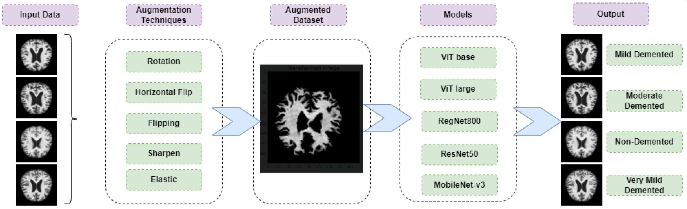
This study focuses on medical image analysis and aims to support the early diagnosis of Alzheimer’s disease from structural brain imaging. An overview of the proposed framework is shown in Figure 1. Two open-source datasets from the Alzheimer’s Disease Neuroimaging Initiative (ADNI) were used for training and evaluation. To mitigate class imbalance, data augmentation techniques such as rotation, horizontal flipping, sharpening, and elastic transformations were applied.

We evaluated two ViT variants—ViT-Base and ViT-Large—and compared their performance with CNN-based models including ResNet, RegNet, and MobileNet. Throughout all experiments, the enhanced optimizer was applied consistently to assess its impact on both architectures.

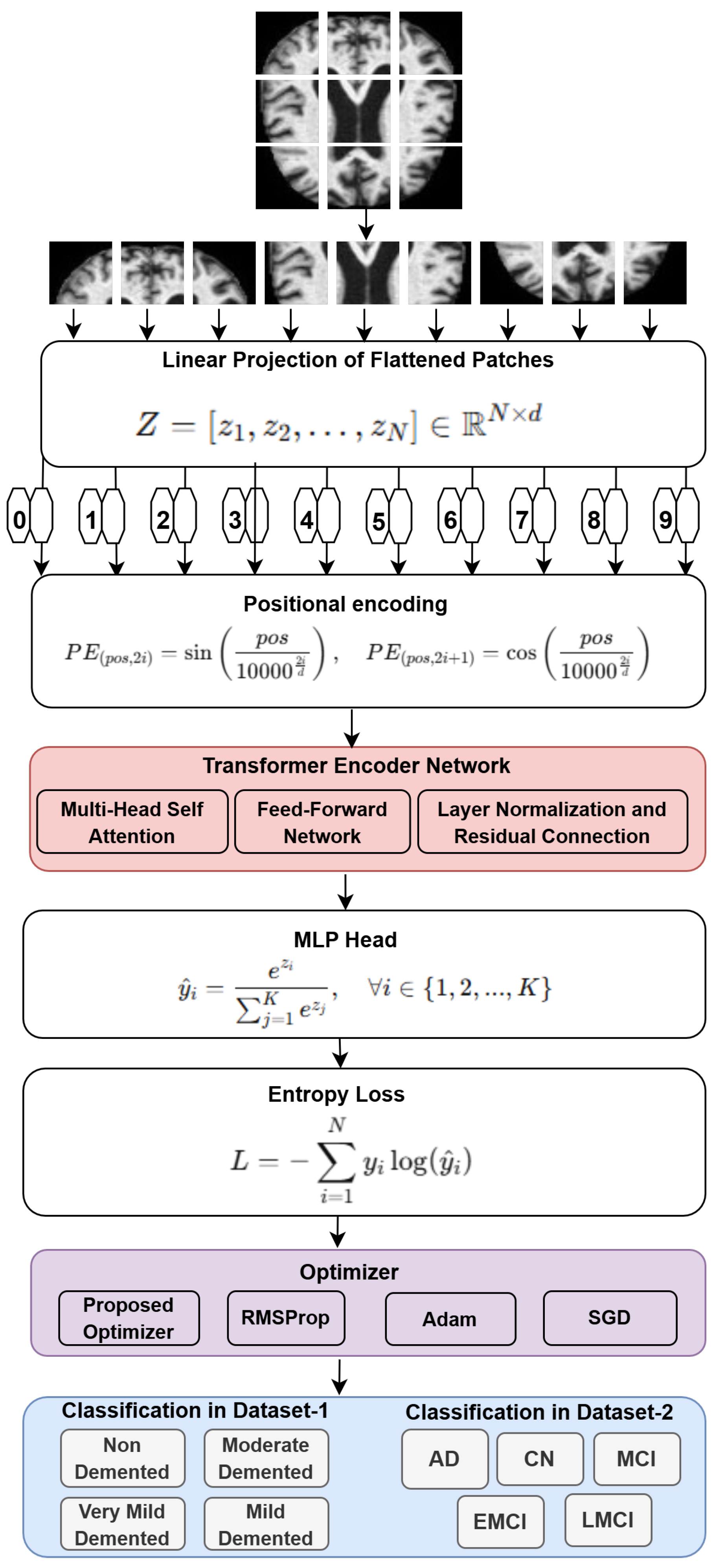
Figure 2 illustrates the detailed ViT architecture used in this study. The model processes input MRI images by dividing them into non-overlapping patches, which are then flattened and passed through a linear projection layer to generate patch embeddings. These embeddings are combined with positional encodings—computed using sinusoidal functions—to preserve spatial information lost during tokenization.

The resulting sequence is fed into the Transformer Encoder, which consists of stacked layers of Multi-Head Self-Attention (MHSA) and feed-forward networks. This allows the model to learn long-range dependencies and spatial relationships across the image.

A Multi-Layer Perceptron (MLP) head follows the encoder and includes fully connected layers for classification, ending with a Softmax layer to output class probabilities. The entropy loss function is used to guide optimization, where lower values reflect more confident predictions.

The key innovation lies in the optimizer: the enhanced Adam variant integrates adaptive learning rate scaling, momentum correction, and decay modulation. This optimizer is designed to accelerate convergence while maintaining stability, and it is empirically shown to outperform conventional optimizers in terms of classification accuracy, entropy loss, and training efficiency.

While the proposed architecture and optimization strategy remained consistent across both datasets, certain experimental design decisions varied due to dataset-specific properties. Dataset-1 comprises four classes representing progressive stages of dementia, with relatively uniform class distributions. In contrast, Dataset-2 features five diagnostic labels—including EMCI and LMCI—which are inherently imbalanced and more nuanced in clinical representation. This class imbalance necessitated heavier reliance on augmentation techniques and adaptive training schedules to prevent overfitting and to improve representation learning for underrepresented categories.

Additionally, Dataset-2 required more aggressive data normalization and enhancement steps due to variability in image quality and acquisition conditions. Although model architectures (ViT, ResNet, RegNet, MobileNet) and optimizers (SGD, RMSProp, Adam, and the proposed enhanced Adam) remained the same across both datasets, training hyperparameters and augmentation intensities were adjusted to ensure that each model effectively captured relevant patterns. These adjustments were crucial to maintaining fairness and validity in comparative evaluations while accounting for the structural differences in the datasets.

3.1. Enhanced Optimizer

In all optimizers, the learning rate serves to alter the weights of the neural network relative to the loss gradient. Lower values represent a gradual decrease/increase in the learning process. The reason for keeping the learning rate low is to ensure that the optimizer does not miss the local minima [38]. On the other hand, convergence also increases proportionally. The default Adam optimizer has two hyperparameters. The Adam optimizer uses the first hyperparameter of momentum and the second hyperparameter of RMSProp [39]. RMSProp does not use the learning rate as a hyperparameter but rather the adaptive learning rate. This causes the learning rate of RMSProp to vary over time. The Adam optimizer is widely used in deep learning due to its adaptive moment estimation technique, which helps in efficient parameter updates. However, traditional Adam suffers from stability and generalization issues in certain scenarios [40,41]. To address these limitations, we propose an “Enhanced Adam Optimizer” with an adaptive learning rate scaling mechanism.

Table 1. Key enhancements in Adam optimizer.

Enhancement	Description	Observed Effects
Adaptive Learning Rate	Learning rate adjusts dynamically with training.	Improved stability, faster convergence.
Momentum Correction	Adjusts moment estimates based on gradient flow.	Enhanced generalization.
Decay Modulation	Regulates learning rate decay based on variance.	Robust convergence, reduced oscillation.

shows the key enhancement made to the Adam optimizer.

Algorithm 1 presents the pseudo-code of the proposed enhanced Adam optimizer. While the algorithm preserves the foundational principles of the original Adam, it introduces an adaptive scaling factor $\gamma$ to modulate the learning rate dynamically. This enhancement is aimed at reducing the impact of large gradient variances, resulting in more stable and consistent convergence—especially in deep learning scenarios.

The algorithm begins by initializing the model parameters ${\theta }_0$ along with the moment vectors $m_0$ and $v_0$, and the training step counter t. It uses the standard hyperparameters of Adam—base learning rate $\alpha$, exponential decay rates ${\beta }_1$ and ${\beta }_2$, and a small constant $ϵ$—to prevent division by zero. Additionally, the proposed method introduces a novel scaling factor $\gamma$.

At each iteration

• The gradient $g_t$ of the objective function is computed.
• Biased first and second moment estimates, $m_t$ and $v_t$, are updated using exponential moving averages.
• Bias correction is applied to obtain ${\widehat{m}}_t$ and ${\widehat{v}}_t$.
• The adaptive learning rate is then computed as

  $${\eta }_t=\alpha ·{\displaystyle \frac{1}{1+\gamma ·{\widehat{v}}_t}}$$

  (8)
  This formulation reduces the step size in regions where the second moment ${\widehat{v}}_t$ is large, thus controlling oscillations and preventing overshooting.
• Finally, the parameters are updated using

  $${\theta }_t={\theta }_{t-1}-{\eta }_t·{\displaystyle \frac{{\widehat{m}}_t}{\sqrt{{\widehat{v}}_t}+ϵ}}$$

  (9)

Overall, this enhancement refines the Adam optimizer by incorporating a variance-sensitive learning rate modulation, making it more robust for training deep neural networks with highly dynamic gradient behaviors.

Algorithm 1 Pseudo-code for the enhanced Adam optimizer.

1: Initialize: Parameters ${\theta }_0$, first moment vector $m_0=0$, second moment vector $v_0=0$, step counter $t=0$ 2: Hyperparameters: Learning rate $\alpha$, decay rates ${\beta }_1,{\beta }_2\in [0,1)$, small constant $ϵ$, scaling factor $\gamma$ 3: for each training iteration do 4:     $t\leftarrow t+1$ 5:     Compute gradient: $g_t={\nabla }_{\theta }J\left({\theta }_{t-1}\right)$ 6:     Update biased first moment estimate: $m_t={\beta }_1{m}_{t-1}+(1-{\beta }_1)g_t$ 7:     Update biased second moment estimate: $v_t={\beta }_2{v}_{t-1}+(1-{\beta }_2)g_t^2$ 8:     Compute bias-corrected moments: $${\widehat{m}}_t={\displaystyle \frac{m_t}{1-{\beta }_1^t}},{\widehat{v}}_t={\displaystyle \frac{v_t}{1-{\beta }_2^t}}$$ 9:     Compute adaptive learning rate: $${\eta }_t=\alpha ·{\displaystyle \frac{1}{1+\gamma ·{\widehat{v}}_t}}$$ 10:     Update parameters: $${\theta }_t={\theta }_{t-1}-{\eta }_t·{\displaystyle \frac{{\widehat{m}}_t}{\sqrt{{\widehat{v}}_t}+ϵ}}$$ 11: end for 12: Return: Optimized parameters ${\theta }_t$

3.2. Experimental Environment

This section provides the details of tools and technologies used while experimenting, implementing, and evaluating the proposed optimization methods against the respective neural network models. In this section, the explanation of the experimental setup and obtained results during the training and testing procedure of the deep neural network is provided as follows.

Training Environment

In this study, we utilized an AMD Ryzen 9 processor with 16 cores and a base clock speed of 3.4 GHz. For GPU acceleration, we employed an NVIDIA GeForce RTX 2080. The development environment consisted of Python 3.12 programming language, with coding performed in PyCharm and Jupyter Notebooks for experimentation and analysis.

We evaluated five different deep learning models: ViT-Base, ViT-Large, RegNet-Y800, ResNet-50, and MobileNet-V3. Each model was trained using three optimizers: enhanced optimizer, Stochastic Gradient Descent (SGD), and RMSProp.

3.3. Model Selection

The models selected for benchmarking—ViT, ResNet, RegNet, and MobileNet—are widely adopted and representative of diverse architectural paradigms (transformer-based, residual, regularized, and lightweight networks). These models remain relevant in the current literature and provide a balanced foundation to evaluate the effectiveness of our proposed optimizer. While several newer classification architectures have emerged, the chosen models offer a strong, interpretable baseline and facilitate meaningful comparisons across varying levels of network complexity.

3.4. Optimizer Selection

In this study, we compared the proposed enhanced Adam optimizer against three widely adopted baseline optimizers: Stochastic Gradient Descent (SGD), RMSProp, and Adam. These optimizers were selected because they form the foundation of most modern adaptive optimization methods and are extensively used in deep learning pipelines across various domains, including medical imaging. Our goal was to establish a reliable and interpretable baseline, enabling a clear and meaningful assessment of the improvements introduced by our optimizer.

While more recent variants such as NAdam and AdamW exist, they are often incremental modifications over Adam and typically target specific tasks or training constraints. To keep the evaluation broadly applicable and focused, we limited our scope to foundational optimizers, ensuring fair and consistent benchmarking across all selected deep learning models.

As shown in our experimental results, the proposed optimizer consistently outperformed the standard methods across different architectures (e.g., ViT, ResNet, MobileNet) and datasets. This demonstrates the general effectiveness of our enhancements, including adaptive learning rate scaling and momentum correction. Future work will explore additional comparisons with other advanced optimizers, such as NAdam, AdamW, and others, to further validate the generalizability and robustness of our method in a wider range of scenarios.

3.5. Dataset

In this section, we provide the details of both datasets used in experimentation for the evaluation purpose. We used two datasets differing mainly based on labeled classes. Each dataset is explained in its respective subsection as follows.

3.5.1. Dataset-1

Dataset-1 was obtained from a publicly available Kaggle repository titled “Alzheimer’s Disease Multiclass Images Dataset”. It contains preprocessed and augmented structural MRI brain scans categorized into four distinct classes: Non Demented, Very Mild Demented, Mild Demented, and Moderate Demented. Each class represents a progressively worsening stage of cognitive impairment, enabling multiclass classification of Alzheimer’s Disease. The dataset includes approximately 44,000 T1-weighted axial MRI slices, balanced across categories through augmentation techniques to mitigate class imbalance. All images were resized to uniform spatial dimensions and intensity-normalized to ensure consistency and compatibility with deep learning model inputs. The dataset’s structure supports the robust training and evaluation of classification models in distinguishing between different stages of dementia.

3.5.2. Dataset-2

Dataset-2 was constructed from the Alzheimer’s Disease Neuroimaging Initiative (ADNI) database, a widely used resource in Alzheimer’s research [42]. It comprises multimodal neuroimaging data, including structural T1-weighted MRI scans, with labels derived from expert clinical assessments. This dataset contains five classes: Cognitively Normal (CN), Early Mild Cognitive Impairment (EMCI), Mild Cognitive Impairment (MCI), Late Mild Cognitive Impairment (LMCI), and Alzheimer’s Disease (AD). These labels provide a finer granularity in disease progression compared to Dataset-1. However, the initial distribution was imbalanced, with EMCI and LMCI being underrepresented. To mitigate this issue, data augmentation techniques such as random rotations, flips, and contrast adjustments were employed. Preprocessing steps included skull stripping, resampling to uniform voxel spacing, and intensity normalization. All images were resized to a consistent shape for input to the neural networks. Dataset-2 enables robust training and evaluation across early-to-advanced Alzheimer’s stages, making it valuable for fine-grained classification tasks.

3.6. Data Augmentation

Data augmentation helps in preventing ML and DL models from acquiring irrelevant information. This procedure is required if the dataset is biased and if it is necessary to let the models learn patterns or features from different perspectives and angles. This enhances the performance of the model.

The following sequence of transformations was applied to each training image during augmentation:

• Resizing,
• Cropping,
• Scaling,
• Enhancement,
• Normalization,
• Horizontal and Vertical Flipping,
• Rotation.

Furthermore, different techniques are utilized for this purpose: for example, resizing, normalization, horizontal flip, vertical flip, rotations, enhancement, cropping, and scaling. These are the basic techniques that we used in the process of data augmentation, which resulted in the unbiased dataset, which resulted in optimal classification results.

Resizing is a technique for changing the dimensions of the images. This results in compatibility issues if not handled in the training process. So, the scaling technique was applied following the enhancement technique. The mathematical formula for resizing is shown in Equation (10) as follows:

$$\left({\omega }_{\mathrm{new}},h_{\mathrm{new}}\right)={\displaystyle \frac{\mathrm{M}}{max(\omega ,h)}}(\omega ,h)$$

(10)

Normalization is used for continuously distributing the pixel range from a range of minimum and maximum pixel values. It does not change the shape of an image but the view of an image. The mathematical formula for the normalization technique is shown in Equation (11) as follows:

$$X_{\mathrm{normalized}}={\displaystyle \frac{x-mean\left(x\right)}{x_{max}-x_{min}}}$$

(11)

Flipping the image can be performed either vertically or horizontally. Both were utilized in this work. Vertical flipping means to reverse the active layer; i.e., from top to bottom. Horizontal flipping means to present the image as if it were being reflected from a mirror. In horizontal flipping all the layers of images are transformed horizontally, from left to right or right to left. This way the only changes are in the position of the pixel on x-axis without losing any information. The formula for vertical and horizontal flipping is shown in Equation (12) as follows:

$$\begin{array}{c}Horizontal\left(f\left(x\right)\right)=x^2\\ Vertical\left(f\left(x\right)\right)=\sqrt{x}\end{array}$$

(12)

Rotation is a method used to rotate an object around the center, which simply means rotating an image in a clockwise or counterclockwise direction. However, we rotated the images in a clockwise direction to generate new images.

Cropping was also utilized while resizing the images. This is required to avoid losing useful information, and the second reason was that scaling is required after cropping, and the enhancement is required in order to not lose useful information. Resizing back to the same dimensions was a necessary step, as the training process smoothly ran without issues and was fast.

Enhancement is a necessary step if the resizing of images is performed. As a result of resizing or cropping, images might need to be scaled back to the original dimensions due to which the quality of the image might be affected. To address this challenge, image enhancement is used. This is performed to avoid noise from an image. The mathematical formulae shown in Equation (13) for enhancement is as follows:

$$g(x,y)=\left\{\begin{array}{c}{a}_{1}f(x,y)f(x,y)<r_1\\ \left.a_2\left(f(x,y)-r_1\right)+s_1,r_1\ge f(x,y)<r_2\right)\\ a_3\left(f(x,y)-r_2\right)+s_2,f(x,y)<r_3\end{array}\right.$$

(13)

In the above Equation (13), $g(x,y)$ is the output of the image, while $f(x,y)$ is the input pixel data, where $a_1$, $a_2$, and $a_3$ are scaling factors for many grayscale areas and $s_1$, $s_2$, $r_1$, and $r_2$ are the adjustable parameters.

Figure 3 shows a sample of an original image from the dataset over which transformation was applied. The image to the right is the result of the full augmentation sequence. Although the transformation modifies the view of images significantly, it does not lose the characteristics that are used in AD classification.

4. Results

In this section, we briefly explain the results achieved during the experiments performed.

Table 2. Training and testing accuracies against dataset-1.

Model	Optimizer	Training Accuracy	Testing Accuracy
ViT-base	Modified Optimizer	99.94%	99.84%
	SGD	74.68%	79.34%
	RMSProp	51.70%	55.71%
ViT-large	Modified Optimizer	99.84%	99.84%
	SGD	82.73%	87.94%
	RMSProp	50.03%	50.07%
RegNet-Y800	Modified Optimizer	99.92%	99.00%
	SGD	53.22%	56.96%
	RMSProp	98.72%	98.84%
ResNet-50	Modified Optimizer	99.81%	99.12%
	SGD	50.55%	52.42%
	RMSProp	97.88%	97.84%
MobileNet-v3	Modified Optimizer	99.71%	98.37%
	SGD	54.19%	56.65%
	RMSProp	95.48%	96.43%

and

Table 3. Training and testing accuracies against dataset-2.

Model	Optimizer	Training Accuracy	Testing Accuracy
ViT-base	Modified Optimizer	99.46%	95.75%
	Adam	96.15%	92.18%
	AdamW	99.40%	90.20%
	SGD	63.92%	61.47%
	RMSProp	53.70%	55.52%
ResNet-50	Modified Optimizer	99.59%	94.05%
	Adam	99.45%	93.13%
	AdamW	97.03%	93.80%
	SGD	50.03%	50.07%
	RMSProp	98.03%	90.07%

depict the results of multiple models with variants of several optimizers; e.g., modified optimizer, SGD, RMSProp, and Adam. Each optimizer was configured for the purpose of evaluating its training and validation accuracies, entropy loss, and total training time. It is evident that the modified optimizer was applied over each model and provided better performance overall; i.e., less training time, higher accuracy, and less entropy loss for both training and validation. For Vit-base, Vit-large, RegNet-Y800, ResNet-50, and MobileNet-v3, the respective training times are also considered to be the best when trained with the modified optimizer. There is a little negligible and higher training time difference in some cases when the modified optimizer is compared to SGD and RMSProp, it but can be neglected because there is a marginal difference in both accuracy and entropy loss. Hence, the modified optimizer can be considered a better candidate when compared to SGD, RMSProp, and Adam.

For a comparison of the chosen optimizers against each model, the Alzheimer’s classification accuracy is higher when the modified optimizer is considered. This statement holds true for both training and validation accuracies. It can also be seen that the training and validation entropy losses for the modified optimizer are lower than the SGD and RMSProp. Finally, from the tabulated results, it is concluded that the modified optimizer results in better performance when evaluated against the provided models, which refers to the fact that it is a better candidate for Alzheimer’s classification overall.

Table 2 presents a comparison of ViT-base, ViT-large, RegNet, MobileNet and ResNet. Both the models were trained using three different optimizers; i.e., modified optimizer, SGD, and RMSProp. This table includes training and testing accuracy and training and testing entropy loss results against dataset-1. It can be concluded that both models performed better when the modified optimizer was used.

Table 3 presents a comparison of ViT-base and ResNet. Both models were trained using four different optimizers: i.e., modified optimizer, SGD, RMSProp, and Adam. This table includes training and testing accuracy and training and testing entropy loss results against dataset-2. It can be concluded that both models performed better when the modified optimizer was used.

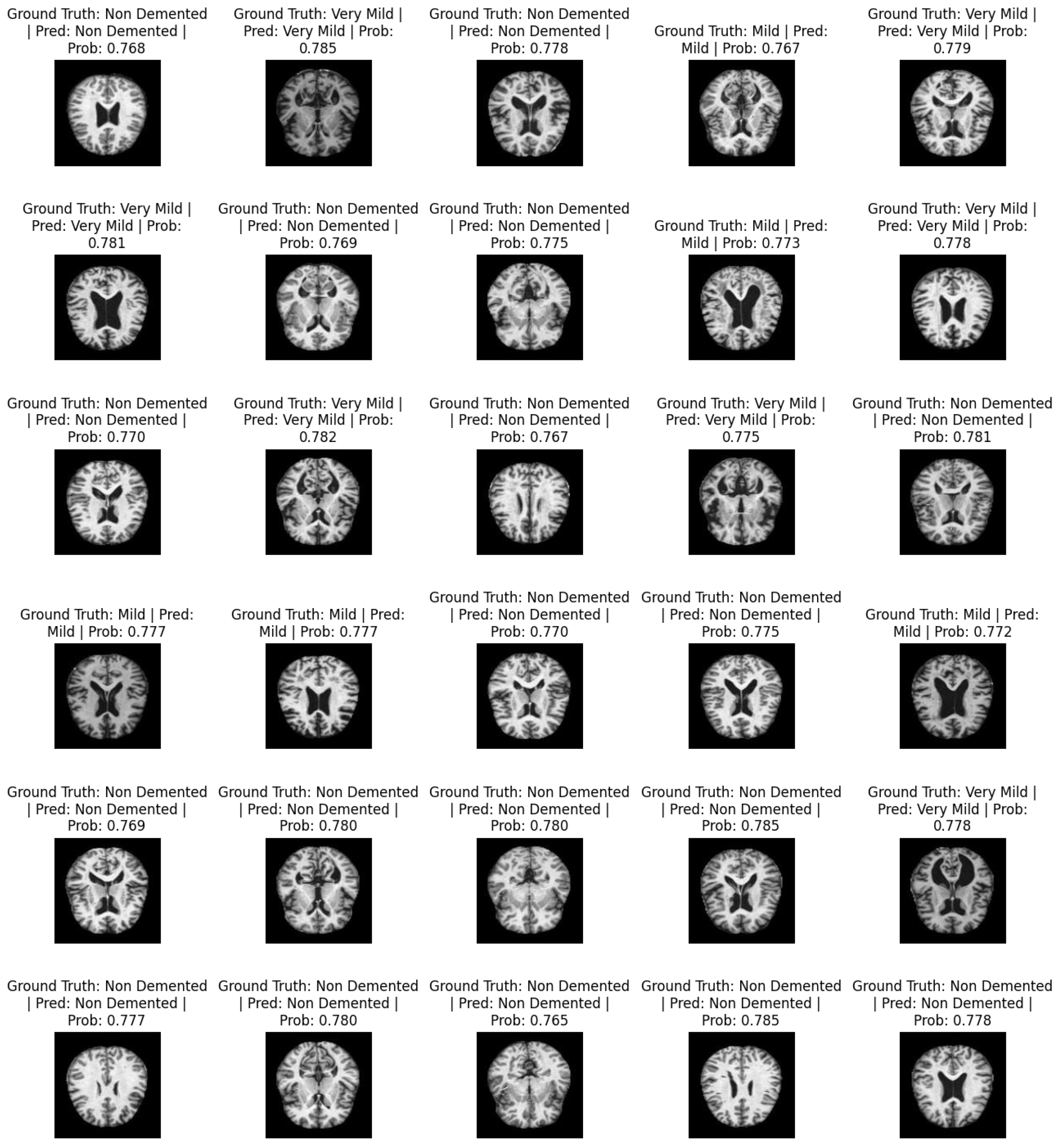
Figure 4 shows a sample of predicted images. It contains information about the actual labels and predicted labels: i.e., ground truth and prediction. For each image, the classification probabilities ranging from 0 and 1 show the probability of the image being classified as one of the respective classes. The total number of classes is non-demented, mild, moderate demented, and very mild.

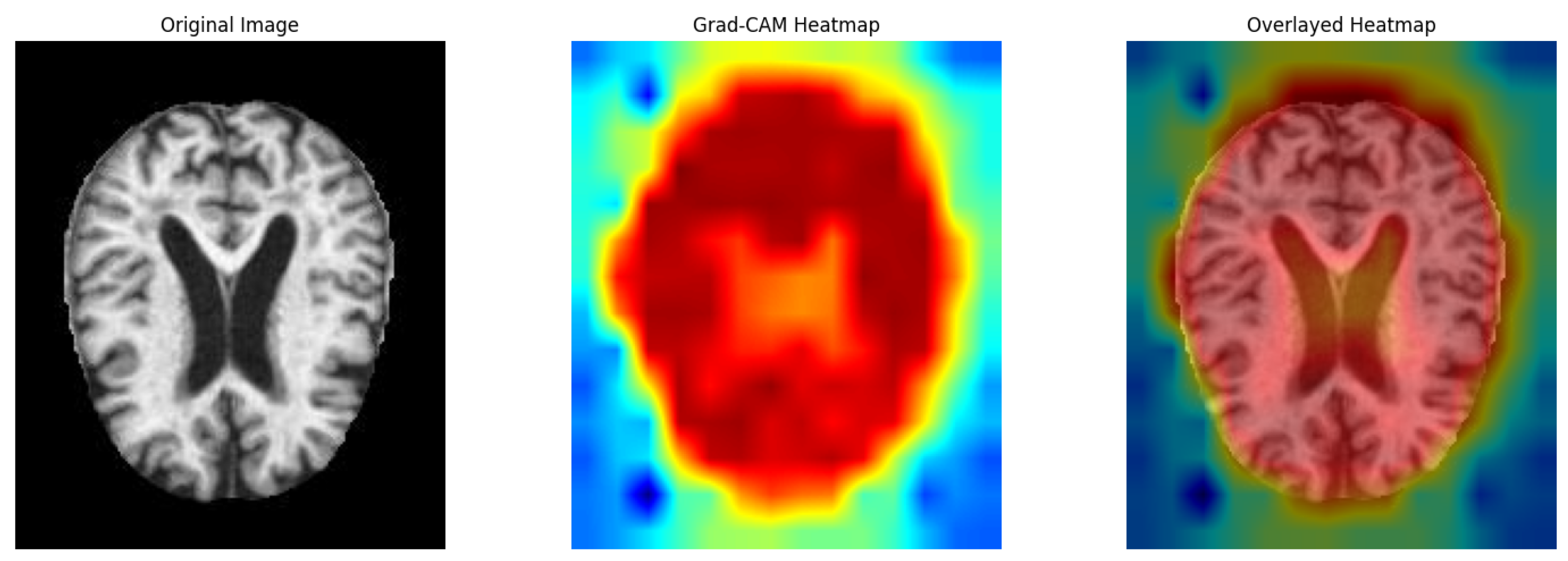
To provide deeper insights into the model’s decision-making process, we employed Grad-CAM (Gradient-weighted Class Activation Mapping) to visualize the areas of the input image that contribute most significantly to the classification output. Figure 5 illustrates three images: (1) the original brain MRI image, (2) the Grad-CAM heatmap showing activated regions, and (3) the overlay of the heatmap on the original image.

As observed, the model predominantly focuses on the ventricular regions and surrounding cortical structures, which are clinically associated with Alzheimer’s disease. The red regions in the heatmap indicate high activation, suggesting that the model assigns greater importance to these areas during classification. In contrast, cooler regions correspond to areas with less contribution to the prediction.

This visualization validates that the proposed model learns relevant neuroanatomical features rather than relying on irrelevant background information. The Grad-CAM overlay enhances interpretability and supports the robustness of the proposed optimizer and architecture in highlighting meaningful brain regions.

4.1. ViT-Base (Dataset-1)

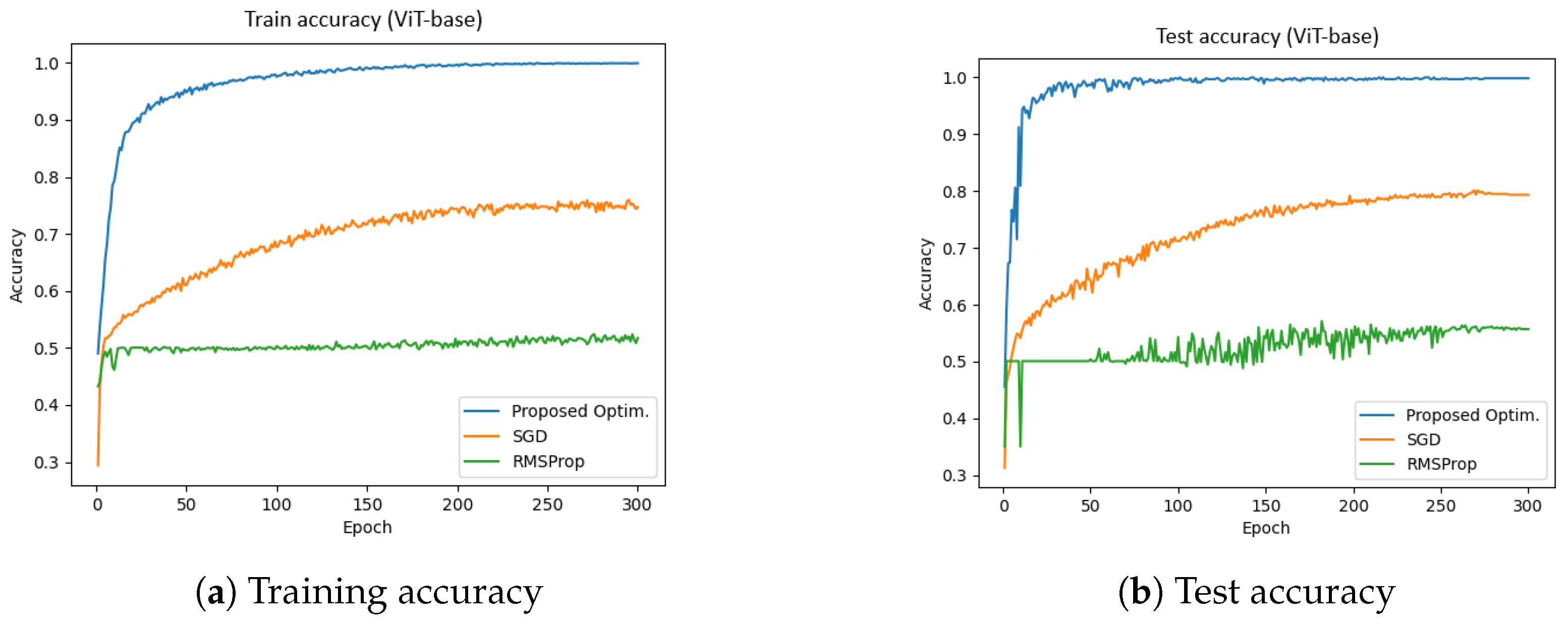
Figure 6 presents the training and test accuracy of the ViT-base model using different optimizers. Figure 6a illustrates the training accuracy, while Figure 6b depicts the test accuracy. The x-axis represents the number of epochs (ranging from 0 to 300), and the y-axis denotes accuracy. The blue, orange, and green curves correspond to the proposed optimizer, SGD, and RMSProp, respectively.

The experiments were conducted using a batch size of 64 and a learning rate of 0.001. The results indicate that the proposed optimizer significantly outperforms SGD and RMSProp in both the training and validation phases. Specifically, the training and validation accuracies achieved by the proposed optimizer were 99.94% and 99.84%, respectively, whereas SGD reached approximately 78%, and RMSProp achieved around 54%.

Furthermore, the total training time for the proposed optimizer, SGD, and RMSProp was 1544.67 s, 1557.26 s, and 1575.23 s, respectively. These results suggest that the proposed optimizer not only enhances accuracy but also improves training efficiency in the ViT-base model.

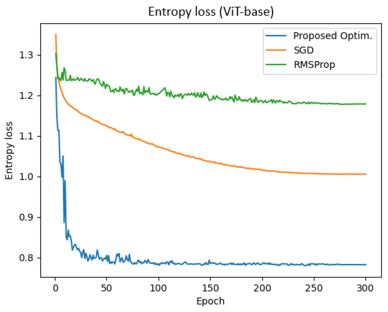
Figure 7 presents the entropy loss of the ViT-base model across training epochs for different optimizers. The x-axis represents the number of epochs (ranging from 0 to 300), while the y-axis denotes the entropy loss. The blue, orange, and green curves correspond to the proposed optimizer, SGD, and RMSProp, respectively.

The experiments were conducted with a batch size of 64 and a learning rate of 0.001. The results demonstrate that the proposed optimizer achieved significantly lower entropy loss compared to SGD and RMSProp. Specifically, the final training and validation entropy losses for the proposed optimizer were 0.781 and 0.782, respectively, whereas SGD and RMSProp yielded entropy losses of approximately 1.005 and 1.178, respectively.

Additionally, the total training time for the proposed optimizer, SGD, and RMSProp was 1544.67 s, 1557.26 s, and 1575.23 s, respectively. These findings indicate that the proposed optimizer not only reduced entropy loss more effectively but also enhanced training efficiency in the ViT-base model.

4.2. ViT-Large (Dataset-1)

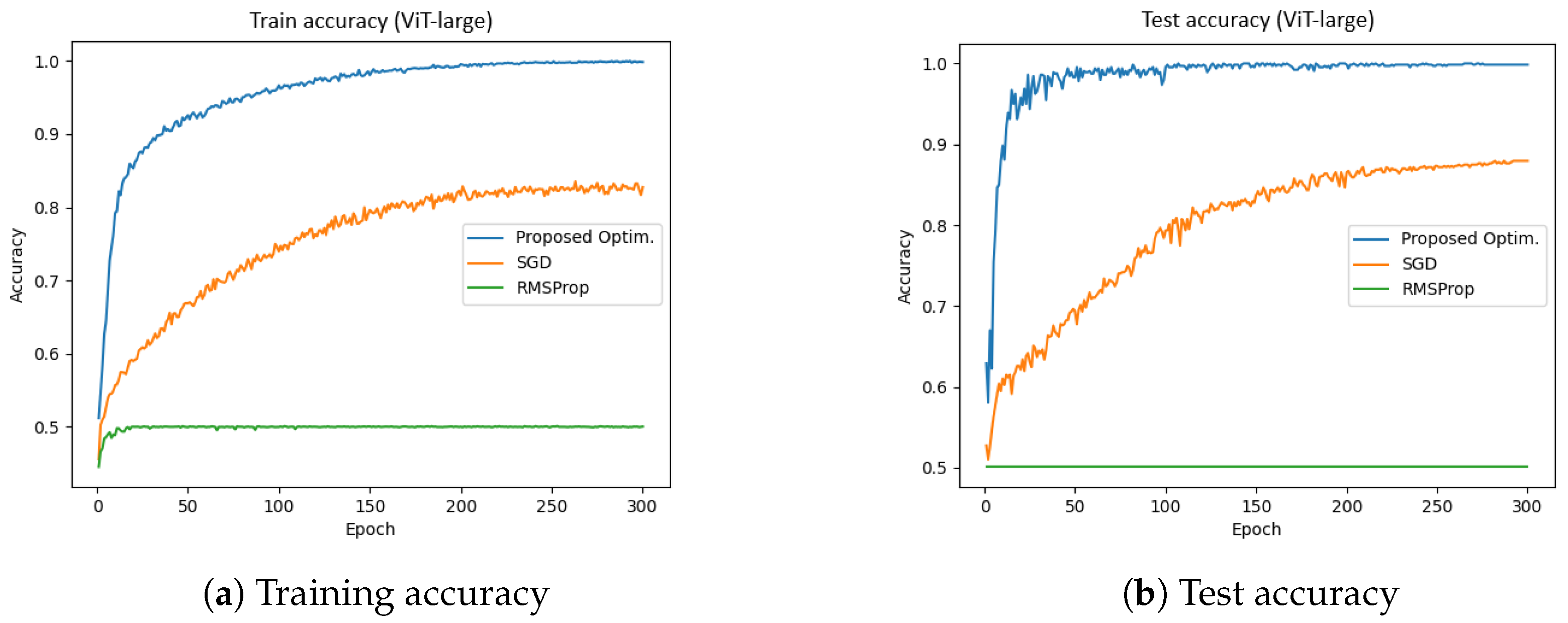
Figure 8 presents the training and test accuracies of the ViT-large model using different optimizers. Figure 8a illustrates the training accuracy, while Figure 8b depicts the test accuracy. The results indicate that the proposed optimizer significantly outperformed SGD and RMSProp in both the training and validation phases. Specifically, the training and validation accuracies achieved by the proposed optimizer were 99.84% and 98.84%, respectively, whereas SGD reached approximately 78%, and RMSProp achieved around 54%. Furthermore, the total training time for the proposed optimizer, SGD, and RMSProp was 4616.22 s, 4606.59 s, and 4475.80 s, respectively. These results suggest that the proposed optimizer not only enhanced accuracy but also improved training efficiency in the ViT-large model.

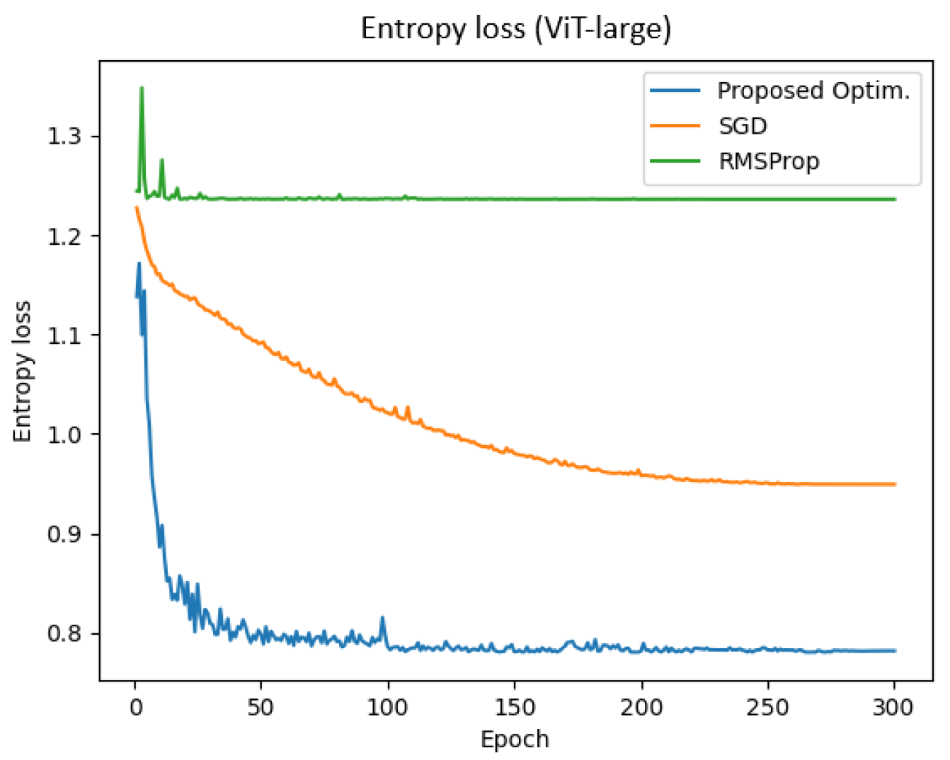
Figure 9 represents the entropy loss of the ViT-large model across training epochs for different optimizers. The results demonstrate that the proposed optimizer achieved a significantly lower entropy loss compared to SGD and RMSProp. Specifically, the final training and validation entropy losses for the proposed optimizer were 0.782 and 0.781, respectively, whereas SGD and RMSProp yielded entropy losses of approximately 0.949 and 1.235, respectively.

Additionally, the total training time for the proposed optimizer, SGD, and RMSProp was 4616.22 s, 4606.59 s, and 4475.80 s, respectively. These findings indicate that the proposed optimizer not only reduced entropy loss more effectively but also enhanced training efficiency in the ViT-large model.

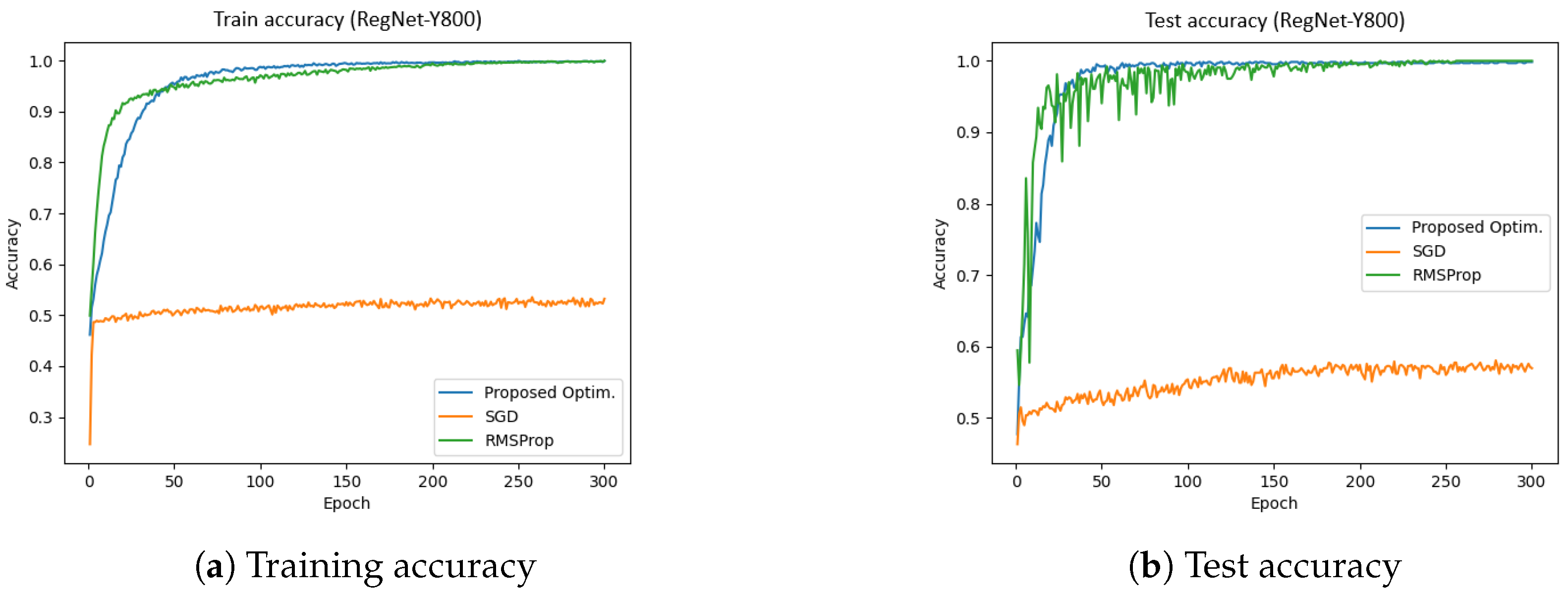
4.3. RegNet-Y800 (Dataset-1)

Figure 10 presents the training and test accuracies of the RegNet-Y800 model using different optimizers. Figure 10a illustrates the training accuracy, while Figure 10b depicts the test accuracy. The results indicate that the proposed optimizer significantly outperformed SGD and RMSProp in both the training and validation phases. Specifically, the training and validation accuracies achieved by the proposed optimizer were 99.92% and 99.00%, respectively, whereas SGD reached approximately 56%, and RMSProp achieved around 98%. Furthermore, the total training time for the proposed optimizer, SGD, and RMSProp was 350.90 s, 351.27 s, and 427.10 s, respectively. These results indicate that the proposed optimizer not only enhanced accuracy but also improved training efficiency in the RegNet-Y800 model.

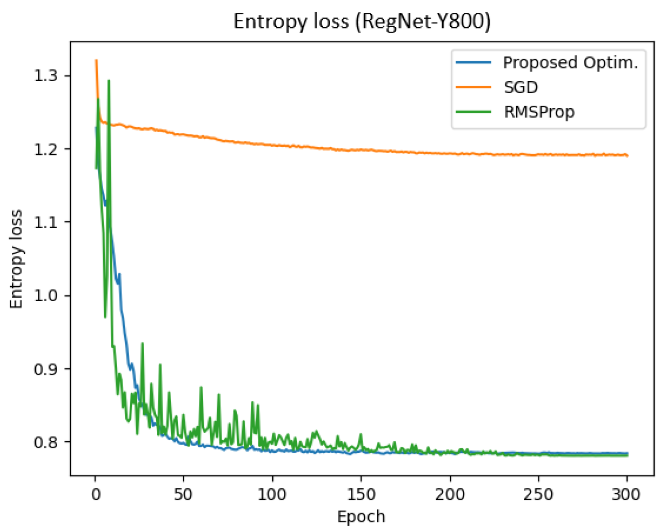
Figure 11 represents the entropy loss of the RegNet-Y800 model across training epochs for different optimizers. The results demonstrate that the proposed optimizer achieved a significantly lower entropy compared to SGD and RMSProp. Specifically, the final training and validation entropy losses for the proposed optimizer were 0.783 and 0.784, respectively, whereas SGD and RMSProp yielded entropy losses of approximately 1.189 and 0.780, respectively.

Additionally, the total training time for the proposed optimizer, SGD, and RMSProp was 350.90 s, 351.27 s, and 427.10 s, respectively. These findings indicate that the proposed optimizer not only reduced entropy loss more effectively but also enhanced training efficiency in the RegNet-Y800 model.

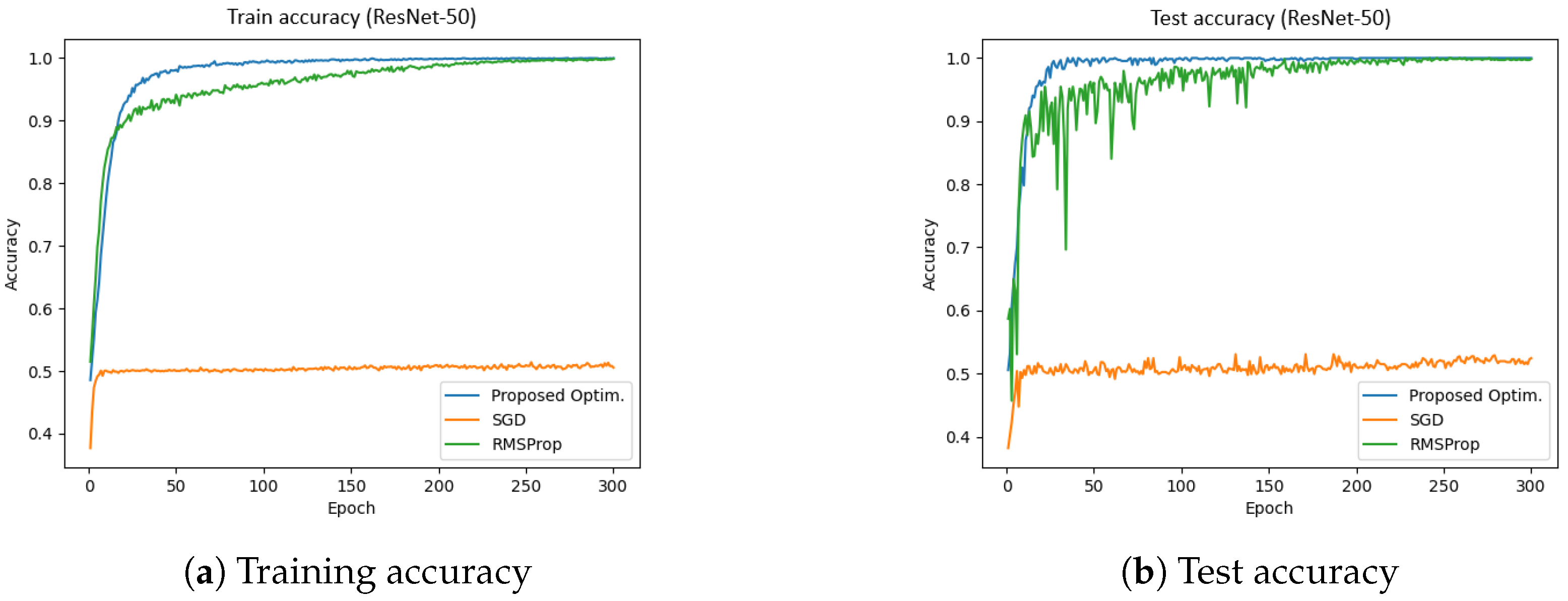
4.4. ResNet-50 (Dataset-1)

Figure 12 presents the training and test accuracies of the ResNet-50 model using different optimizers. Figure 12a illustrates the training accuracy, while Figure 12b depicts the test accuracy. The results indicate that the proposed optimizer significantly outperformed the SGD and RMSProp in both the training and validation phases. Specifically, the training and validation accuracies achieved by the proposed optimizer were 99.81% and 99.12%, respectively, whereas SGD reached approximately 52%, and RMSProp achieved around 97%. Furthermore, the total training time for the proposed optimizer, SGD, and RMSProp was 780.75 s, 770.90 s, and 772.86 s, respectively. These results indicate that the proposed optimizer not only enhanced accuracy but also improved training efficiency in the ResNet-50 model.

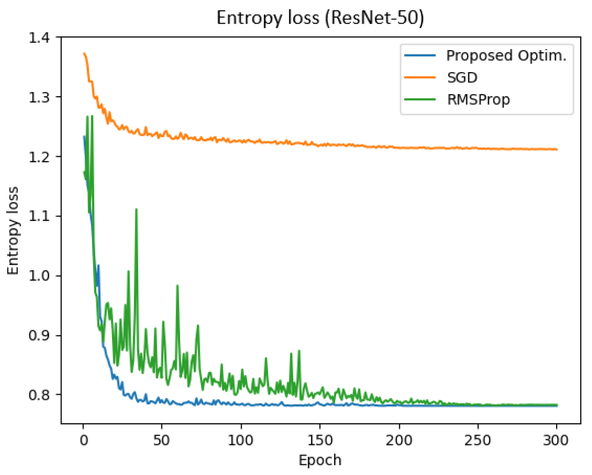
Figure 13 represents the entropy loss of the ResNet-50 model across epochs for different optimizers. The result demonstrates that the proposed optimizer achieved a significantly lower entropy compared to SGD and RMSProp. Specifically, the final training and validation entropy losses for the proposed optimizer were 0.781 and 0.780, respectively, whereas SGD and RMSProp yielded entropy losses of approximately 1.211 and 0.782, respectively.

Additionally, the total training time for the proposed optimizer, SGD, and RMSProp was 780.75 s, 770.90 s, and 772.86 s, respectively. These findings indicate that the proposed optimizer not only reduced entropy loss more effectively but also enhanced training efficiency in the ResNet-50 model.

4.5. MobileNet-v3 (Dataset-1)

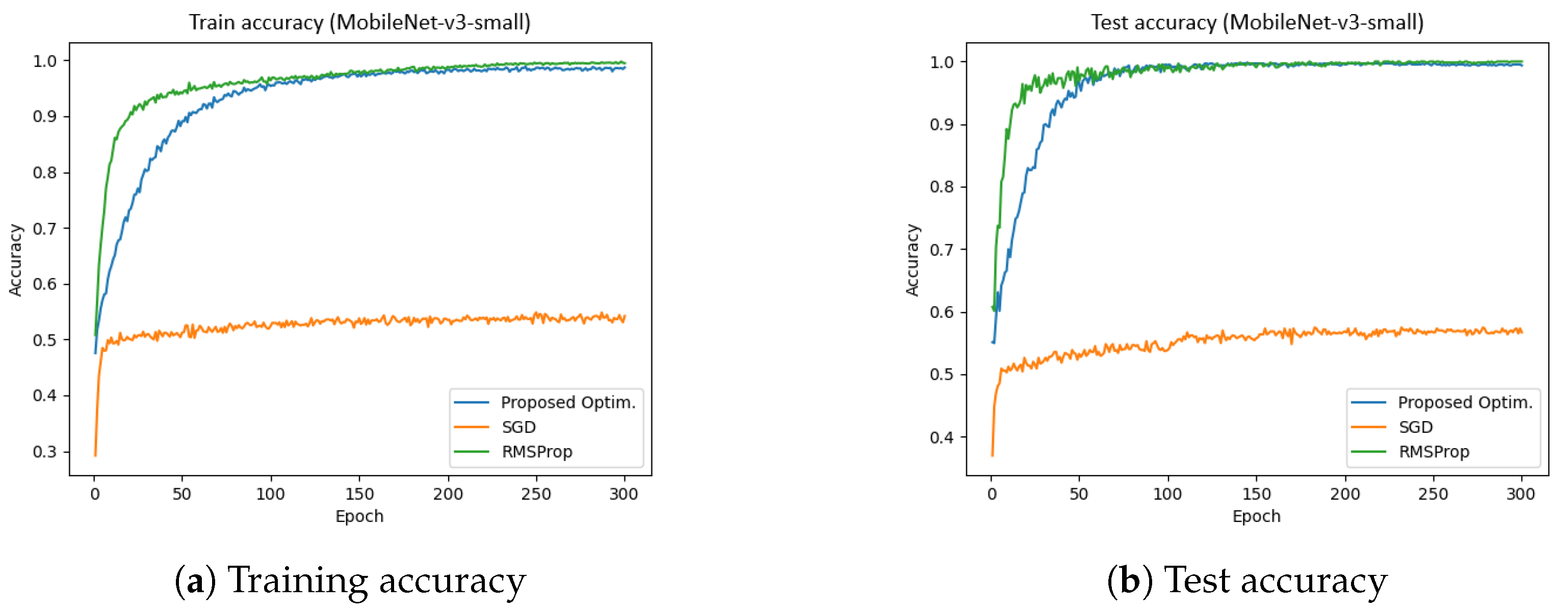
Figure 14 presents the training and test accuracies of the MobileNet-v3 model using different optimizers. Figure 14a illustrates the training accuracy, while Figure 14b depicts the test accuracy. The results indicate that the proposed optimizer significantly outperformed the SGD and RMSProp in both training and validation phases. Specifically, the training and validation accuracies achieved by the proposed optimzers were 98.71% and 99.37%, respectively, whereas SGD reached approximately 54%, and RMSProp achieved around 96%. Furthermore, the total training time for the proposed optimizer, SGD, and RMSProp was 281.95 s, 309.14 s, 290.42 s, respectively. These results indicate that the proposed optimzer not only enhanced accuracy but also improved training efficiency in the MobileNet-v3 model.

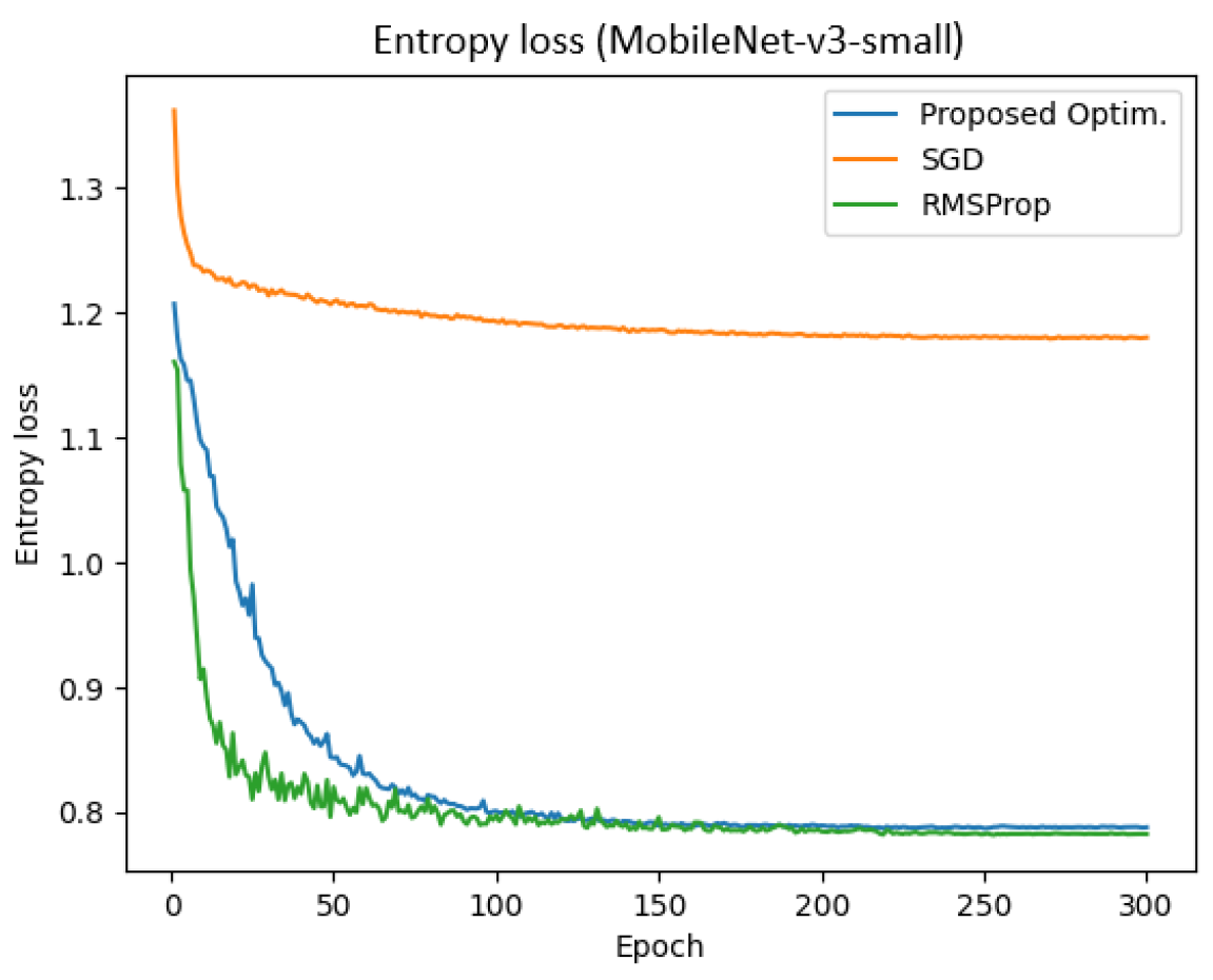
Figure 15 represents the entropy loss of the MobileNet-v3 model across epochs for different optimizers. The result demonstrates that the proposed optimizer achieved a significantly lower entropy compared to SGD and RMSProp. Specifically, the final training and validation entropy losses for the proposed optimizer were 0.801 and 0.787, respectively, whereas SGD and RMSProp yielded entropy losses of approximately 1.180 and 0.782, respectively.

Additionally, the total training time for the proposed optimizer, SGD, and RMSProp was 281 s, 309.14 s, and 290.42 s, respectively. These findings indicate that the proposed optimizer not only reduced entropy loss more effectively but also enhanced training efficiency in the MobileNet-v3 model.

While the proposed optimizer may not have exhibited the fastest initial convergence in terms of early epochs, it achieved lower and more stable final entropy values than SGD and RMSProp. As seen in Figure 15, the curve corresponding to our method descends steadily and maintains reduced entropy, indicating superior long-term convergence quality and reduced variance. This stability is crucial in medical imaging tasks, where generalization and reliability are prioritized over early rapid gains.

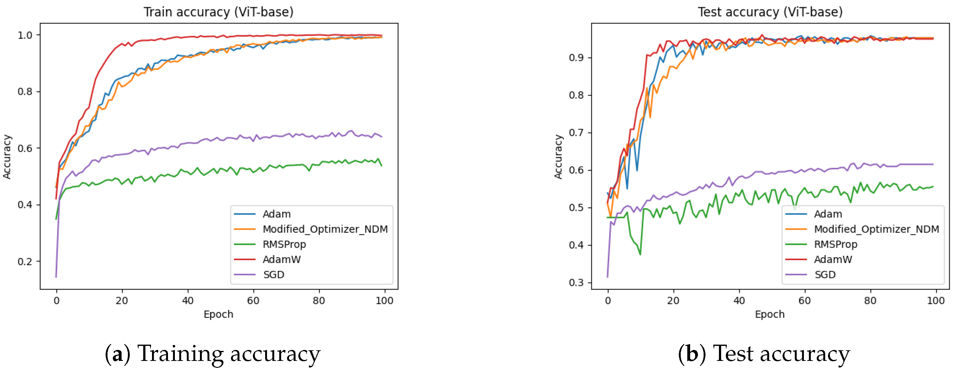
4.6. ViT-Base (Dataset-2)

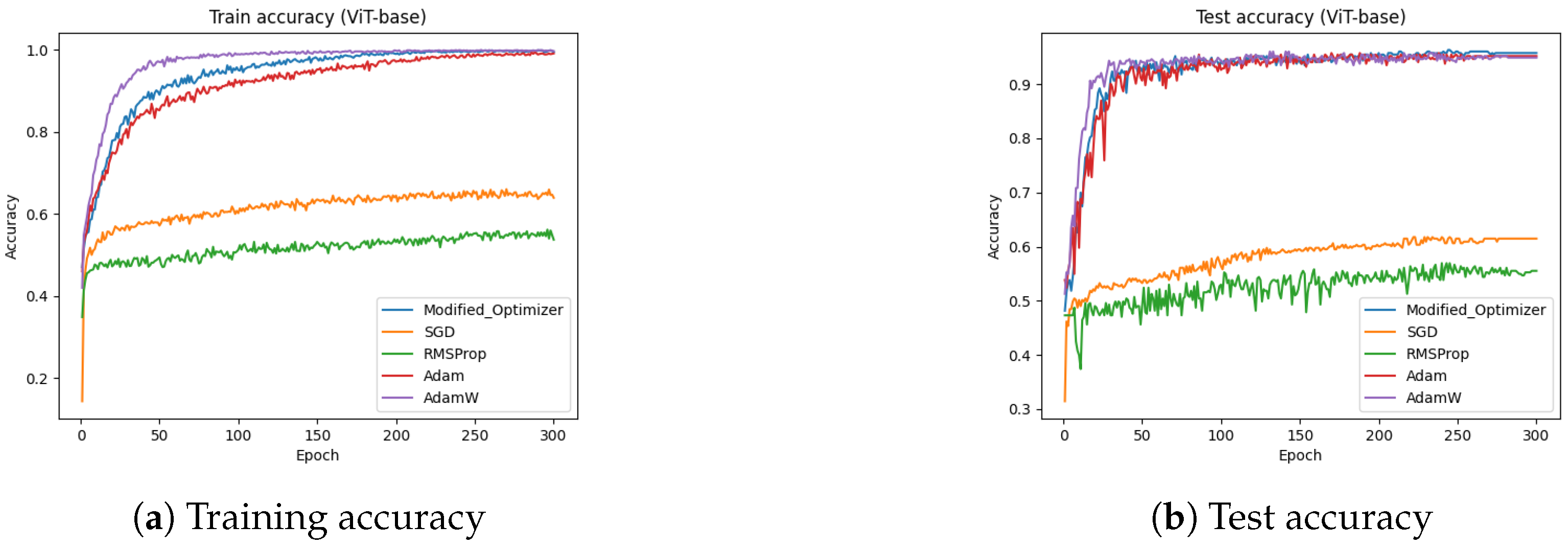
Figure 16 presents the training and test accuracies of the ViT-base model using different optimizers. Figure 16a illustrates the training accuracy, while Figure 16b depicts the test accuracy. The results indicate that the proposed optimizer significantly outperformed the Adam, AdamW, SGD, and RMSProp in both the training and testing phases. Specifically, the training and testing accuracies achieved by the proposed optimizer were 99.46% and 95.75% respectively, whereas Adam reached approximately 92%, AdamW reached approximately 90%, SGD reached approximately 61%, and RMSProp achieved around 55%.

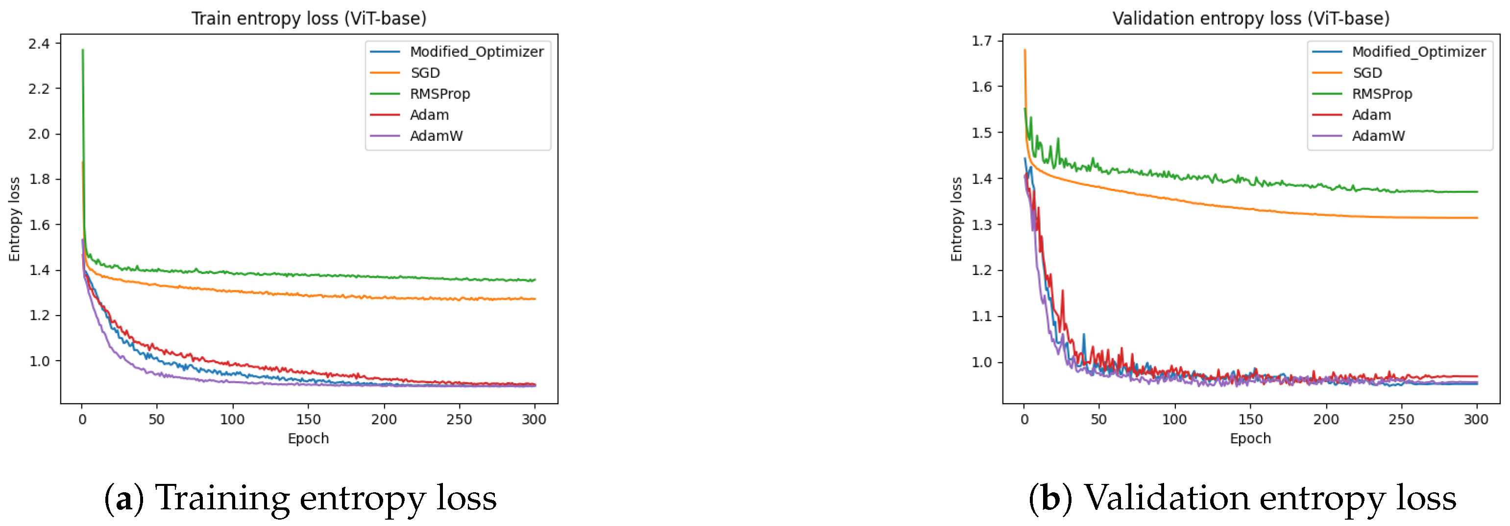
Figure 17 presents the training and test entropy losses of the ViT-base model for different optimizers. The results indicate that the proposed optimizer and Adam achieved a lower entropy loss compared to SGD and RMSProp. The training entropy loss in Figure 17a and test entropy loss in Figure 17b show that both the proposed optimizer and Adam converged faster and reached lower final loss values. These findings reinforce the effectiveness of the proposed optimizer in improving model convergence and generalization.

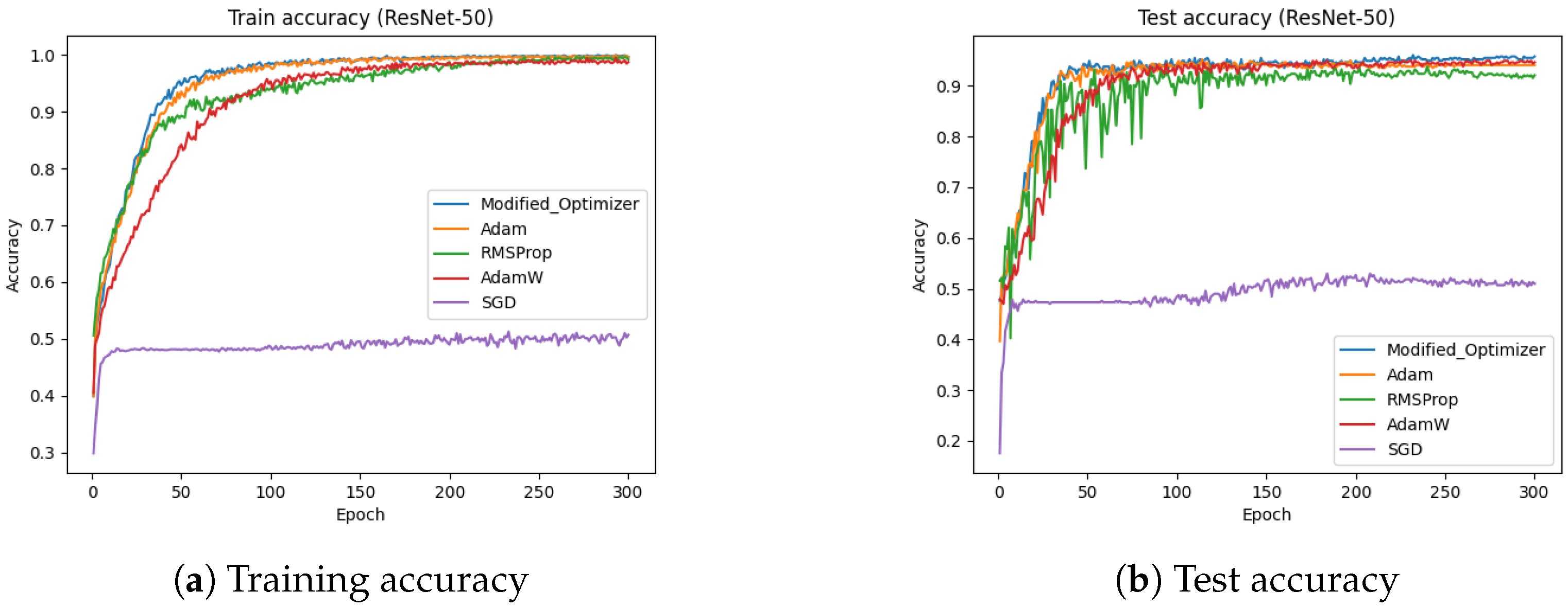
4.7. ResNet-50 (Dataset-2)

Figure 18 presents the training and test accuracies of the ResNet-50 model using different optimizers. Figure 18a illustrates the training accuracy, while Figure 18b depicts the test accuracy. The results indicate that the proposed optimizer significantly outperformed Adam, AdamW, SGD, and RMSProp in both the training and testing phases. Specifically, the training and testing accuracies achieved by the proposed optimizer were 99.84% and 94.05%, respectively, whereas Adam reached approximately 93%, AdamW reached approximately 93.8%, SGD reached approximately 50%, and RMSProp achieved around 92%.

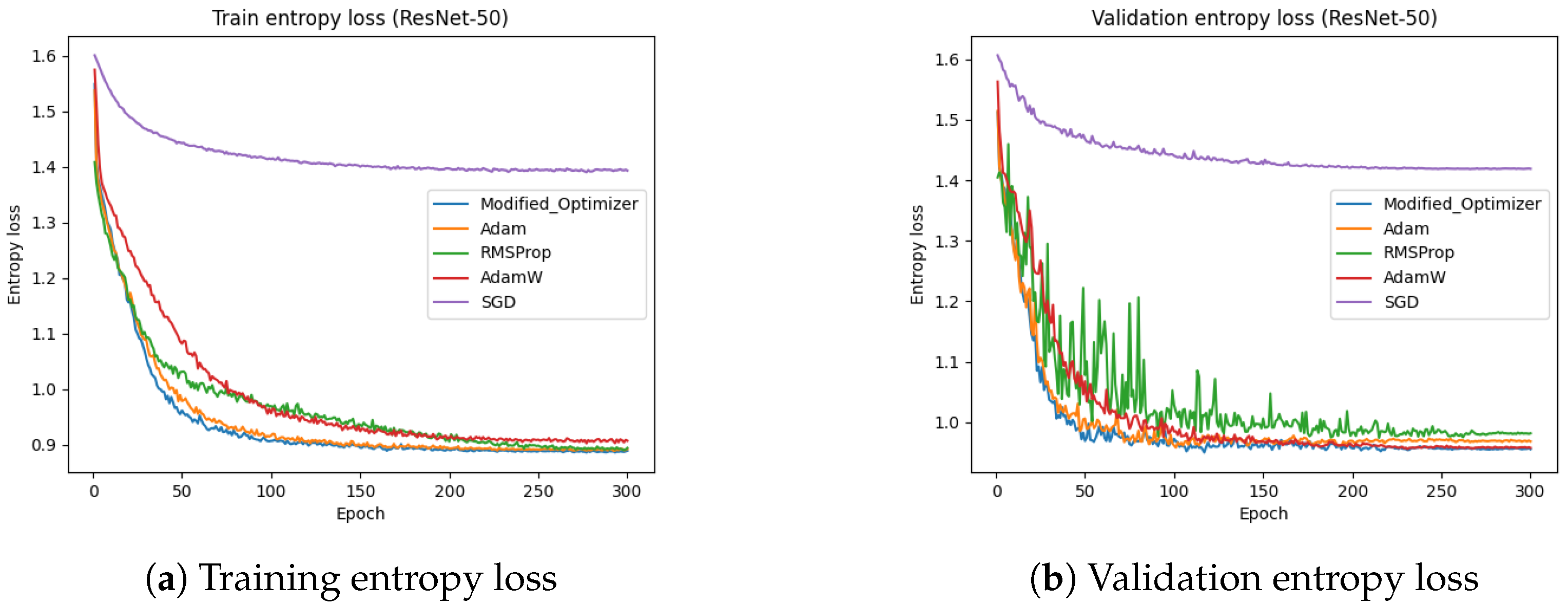
Figure 19 presents the training and test entropy losses of the ResNet-50 model for different optimizers. The results indicate that the proposed optimizer and Adam achieved a lower entropy loss compared to SGD and RMSProp. The training entropy loss in Figure 19a and test entropy loss in Figure 19b show that both the proposed optimizer and Adam converged faster and reached lower final loss values. These findings reinforce the effectiveness of the proposed optimizer in improving model convergence and generalization.

The proposed optimizer demonstrated enhanced training stability across multiple architectures and datasets, as evidenced by significantly lower entropy values and more consistent accuracy outcomes. For instance, as shown in Table 2 and Table 3, models trained with the modified optimizer consistently achieved lower training and testing entropies (≈0.78) compared to SGD and RMSProp (often >1.0), indicating smoother convergence. These results suggest that the optimizer effectively mitigates training noise and stabilizes learning dynamics.

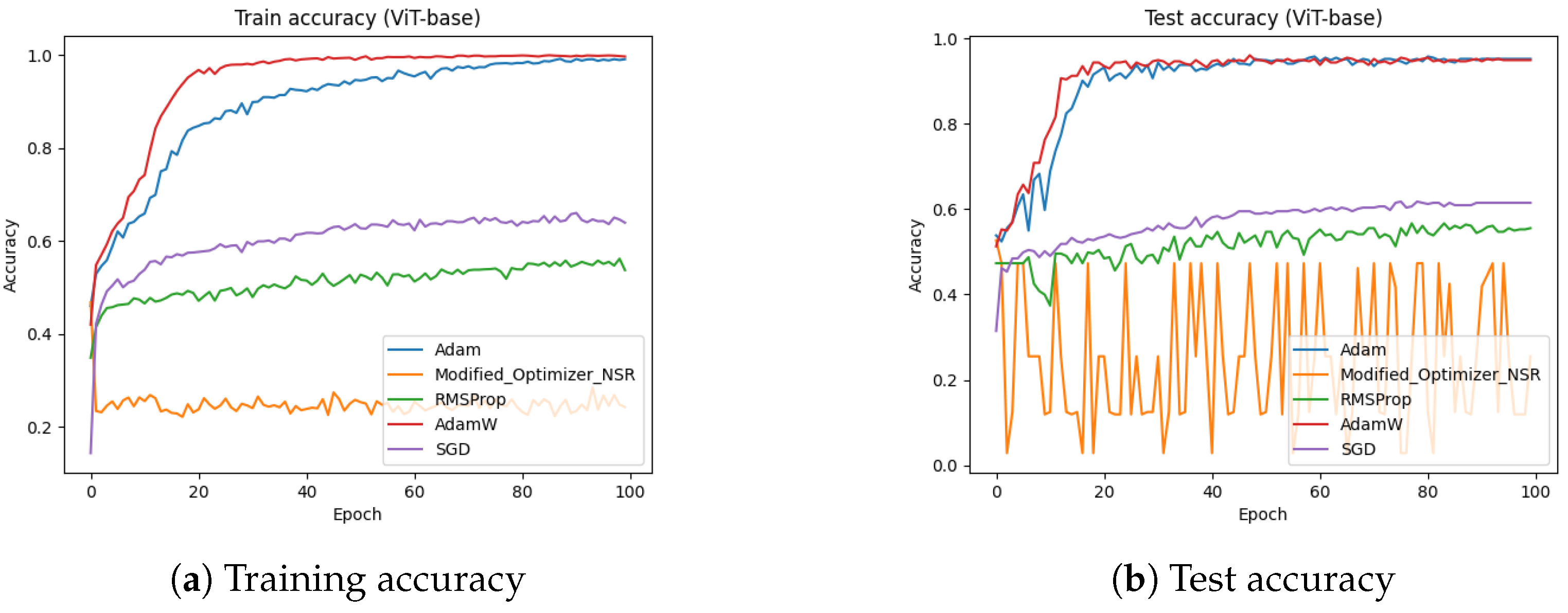
4.8. Ablation Study on Optimizer Components

In this section, we performed an ablation study by disabling the key components in the proposed optimizer and compared the results with state-of-the-art optimizers. We performed the ablation experiment on the ViT-base architecture against dataset-2. Figure 20 shows the effect of disabling the scaling ratio on the training and validation accuracies. In this figure, we can clearly see that the performance of the proposed optimizer significantly drops by disabling the scaling ratio.

Table 4. Ablation experiment on ViT-base against dataset-2.

Variant	Scaling Ratio	Momentum Correction	Decay Modulation	Test Accuracy
Full Optimizer	Yes	Yes	Yes	95%
Without Scaling Ratio	No	Yes	Yes	50%
Without Momentum Correction	Yes	No	Yes	94%
Without Decay Modulation	Yes	Yes	No	93%

presents the testing accuracy of the proposed optimizer against disabling each component.

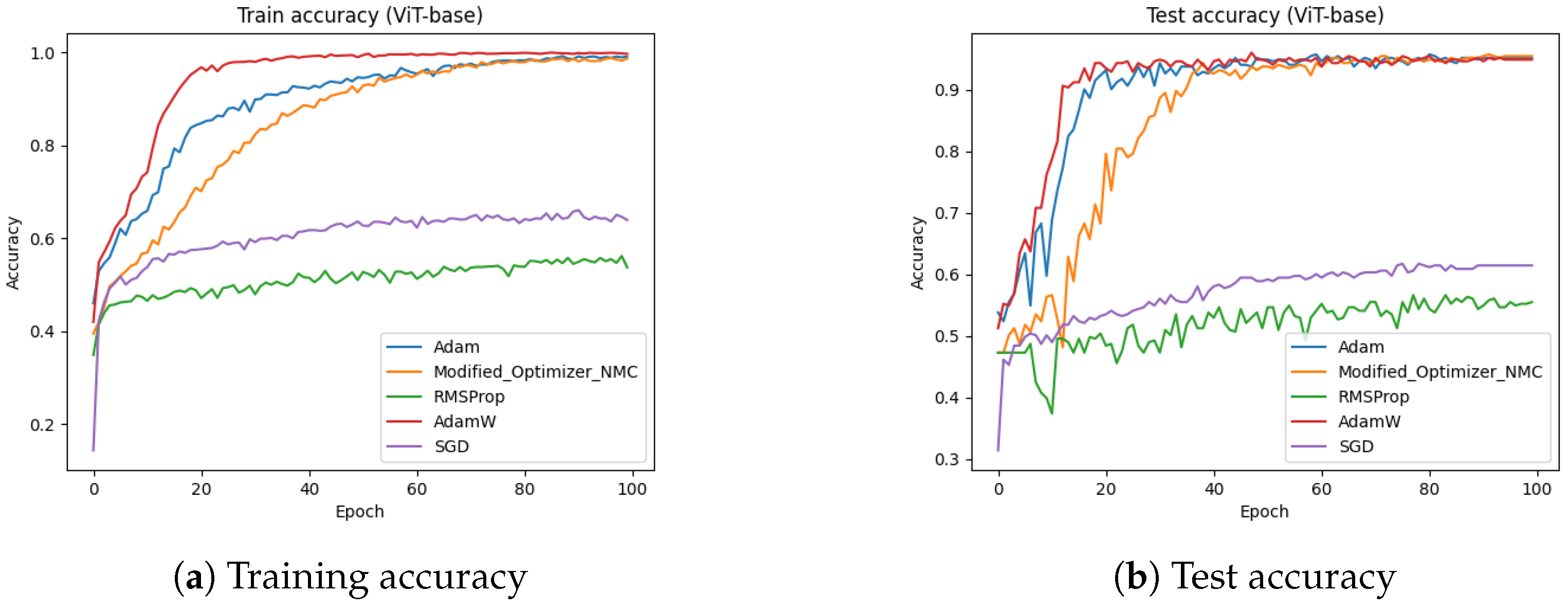
Figure 21 presents the impact of removing momentum correction on the proposed optimizer. In this figure, we can clearly see that by disabling the momentum correction, the performance marginally drops.

Figure 22 presents the absence of decay modulation in the proposed optimizer. In this figure, we can clearly see that by disabling decay modulation, the performance marginally drops in the proposed optimizer.

5. Discussion

This study proposes an enhanced Adam-based optimizer featuring adaptive learning rate scaling, momentum correction, and decay modulation to improve the stability and generalization of deep learning models, particularly in Alzheimer’s disease classification. The optimizer was evaluated across four architectures—ViT, ResNet, RegNet, and MobileNet—demonstrating a superior convergence behavior and classification accuracy when compared to widely used baselines such as Adam, AdamW, SGD, and RMSProp.

We also acknowledge that the comparative experiments on Dataset 1 and Dataset 2 have minor differences, mainly due to the distinct imaging modalities and sample sizes. The design choices were made to preserve the diagnostic relevance and computational feasibility for each dataset while maintaining rigorous and fair benchmarking.

From the results, we can say that ViT-base and ResNet50 performed well with the modified optimizers. In the ablation study, we chose ViT-base due to its performance with the modified optimizer. We conducted experiments by disabling each component; i.e., scaling ratio, momentum correction, and decay modulation. In this study, we could clearly see that by disabling the scaling ratio, the performance of the modified optimizer significantly dropped. On the other hand, by disabling momentum correction and decay modulation, the performance of modified optimizer marginally dropped. We can conclude that the scaling ratio has a great impact on the modified optimizer, whereas momentum correction and decay modulation have a low impact on the modified optimizer, although all the key components play an important role in improving the accuracy of the modified optimizer.

6. Conclusions

In recent years, Alzheimer’s disease (AD) has emerged as a major global health concern. The World Health Organization (WHO) has raised alarms about its rapidly increasing prevalence, reporting that approximately 55 million people worldwide suffer from dementia—a number projected to rise to 78 million by 2030. Notably, around 70% of dementia cases are attributed to AD. Deep learning models, particularly Convolutional Neural Networks (CNNs), have been widely employed in medical image analysis for detecting neurological and oncological conditions, including brain tumors, Parkinson’s disease, and Alzheimer’s disease. CNNs are particularly effective in learning complex spatial features from brain images for diagnostic and prognostic purposes. More recently, Vision Transformers (ViTs) have been introduced as a promising alternative to CNNs for computer vision tasks, including medical imaging.

In this study, we introduced a ViT-based deep learning framework for AD classification and proposed an enhanced Adam optimizer incorporating adaptive learning rate scaling, momentum correction, and decay modulation to improve training stability, convergence speed, and classification accuracy. Our experiments involved multiple deep learning architectures—including ViT variants, ResNet, RegNet, and MobileNet—and were conducted on two publicly available AD datasets. The results demonstrated that our optimizer consistently outperformed conventional methods such as SGD, RMSProp, Adam, and AdamW. For example, ViT-L achieved an accuracy of 99.84% with the proposed optimizer compared to 87.94% with SGD on Dataset 1. ViT-base achieved an accuracy of 95.75% with the proposed optimizer compared to 92.18% with Adam on Dataset 2. The enhanced optimizer also resulted in a lower entropy loss and faster convergence. In the ablation study, we found that the scaling ratio had great a impact on the performance of the modified optimizer, whereas momentum correction and decay modulation had a low impact on the modified optimizer. Furthermore, our analysis suggests that ViT architectures yield better performance on larger datasets, reinforcing their potential in medical image classification tasks. In future work, we plan to expand our experiments by integrating datasets from multiple sources, incorporating attention-based visualization techniques, and exploring advanced transformer architectures such as ViT-H. Additionally, we aim to further improve the optimizer to enhance training efficiency and reduce computational complexity in large-scale Alzheimer’s disease diagnosis applications.