Abstract
This study investigates a nonlinear Schrödinger equation that includes Kudryashov’s quintic power-law refractive index along with dual-form nonlocal nonlinearity. Employing dynamical systems theory, we analyze the model through a traveling-wave transformation, reducing it to a singular yet integrable traveling-wave system. The dynamical behavior of the corresponding regular system is examined, revealing phase trajectories bifurcations under varying parameter conditions. Furthermore, explicit solutions—including periodic, homoclinic, and heteroclinic solutions—are derived for distinct parameter regimes.
Keywords:
Kudryashov’s quintic power law; refractive index; nonlinear Schrödinger equation; bifurcation; periodic solution MSC:
34C25; 34C37; 35C07
1. Introduction
Nonlinear partial differential equations (NLPDEs) have played an important role in the study of many fields such as physics, chemistry, biology, and engineering. The nonlinear Schrödinger equation (NLSE) is a typical NLPDE that has a wide range of applications in theoretical physics, such as nonlinear optics and ion acoustic waves in plasmas. The NLSE describes the propagation of nonlinear optical waves, particularly short pulses in optical fibers.
In 1999, Radhakrishnan et al. proposed an integrable system of coupled NLSEs with cubic-quintic terms and derived the Lax pairs, conservation quantities, and exact soliton solutions for the proposed integrable model in [1]. In 2006, Zheng studied the numerical approximation of one-dimensional cubic NLSEs on the entire real axis and analyzed the associated numerical issues in [2]. Also, Wazwaz used the tanh method and sine–cosine method to obtain the exact solution of a fourth-order NLSE with cubic and power-law nonlinearities in [3]. In 2009, Zhang and Chen used dynamical systems theory to study a generalized NLSE with m-order dispersion, and they derived compact envelope and isolated mode solutions of the equation in [4]. In 2019, Guo studied a class of multidimensional fourth-order NLSE containing derivatives of unknown functions in nonlinear terms and proved the existence of global weak solutions for an NLSE using the Galerkin method in [5]. In 2022, Zhang et al. used the bifurcation theory method of planar dynamical systems to study the NLSE with m-order dispersion and obtained the bifurcation, homoclinic, and heteroclinic solutions of the phase diagram and the exact periodic solution of the planar dynamical system in [6].
In this paper, we consider NLSEs with Kudryashov’s quintic power law of the refractive index, together with two forms of generalized nonlocal nonlinearity, which is the dimensionless form. In [7], this was given by Ekici as follows:
Here, is the complex-valued nonlinear wave function relative to x and t, and the independent variables x and t are, correspondingly, the spatial and temporal components. b expresses the coefficient of the group’s velocity dispersion, while , for , is the self-phase modulation. The coefficients of two types of nonlocal nonlinearity are and , respectively. m represents the order of the medium’s nonlinear response, which is usually rational numbers, and relates to how strong the nonlinear effect is in a medium. The parameter n denotes the quintic power law of the refractive index’s order and is defined as a rational number. It characterizes the magnitude of higher-order nonlinear corrections to the refractive index. The nonlocal nonlinearity’s range is denoted by r. It is usually a positive real number and relates to the area over which the medium’s nonlinear response is averaged.
Equation (1) was examined in earlier works. In 2021, Kudryashov considered the exact solutions of Equation (1) under the conditions of and and further explored the exact solutions for the two special cases of and in [8]. He employed two variants of the simplest-equation method to find solitary wave solutions. In 2022, Ekici derived the bright, dark, and singular soliton solutions of Equation (1) under the conditions of using the extended Jacobian elliptic function method in [9]. Eldidamony et al. used an improved extended direct algebraic algorithm to study Equation (1) under the conditions of and , and they obtained solitons and other types of solutions in [10]. Also, Samir et al. employed the modified Kudryashov’s method to obtain soliton solutions in a governing model featuring cubic–quintic–septic–nonic (CQSN) self-phase modulation with quadrupled structures in [11]. In 2023, Li et al. investigated Equation (1) under the condition of using a generalized experimental equation scheme and obtained solitary wave solutions. They also investigated the soliton solutions, bright soliton solutions, singular soliton solutions, and periodic wave solutions of the equation in [12]. Shakeel et al. employed the improved -expansion technique to study the solutions of Equation (1) under the condition of , and they obtained various types of solutions, such as periodic soliton solutions, twisted singular soliton solutions, and dark soliton solutions, in [13]. Rabie et al. studied Equation (1) under the condition of using the extended F-expansion method and obtained bright soliton solutions, dark soliton solutions, and singular soliton solutions in [14]. Meanwhile, Ali et al. used two methods—the Sardar subequation technique and a new -expansion approach—to solve Equation (1), obtaining unique optical solitons expressed through trigonometric and hyperbolic functions in [15]. In 2024, Zayed et al. used the enhanced direct algebraic method to study the solutions of Equation (1) under the condition of and obtained the soliton solutions of the system in [16]. Ashraf et al. studied the solutions of Equation (1) under the condition of using symbolic computation and the ansatz function approach, obtaining block solitons, periodic waves, and rogue waves in [17], and Murad developed an optical solution scheme based on the novel Kudryashov method for Equation (1), obtaining optical solutions expressed through exponential and hyperbolic functions that encompass various forms including mixed dark–bright solitons, bell-shaped solitons, bright solitons, and wave-type solitons in [18].
It can be observed that existing research on Equation (1) has primarily focused on the case where , with the auxiliary function method being the predominant approach. Consequently, even for the simplified case of , only solutions of specific forms have been obtained. Therefore, the discussion of the solution to Equation (1) is not complete. In this paper, we will use the method of dynamical systems theory to derive the expression of the exact solution of Equation (1), investigating three distinct cases: (1) Case 1: ; (2) Case 2: ; (3) Case 3: .
Many nonlinear partial differential equations can be reduced to the following general form of planar dynamical systems through traveling-wave transformations [19]:
which has a first integral. If defines a set of real-plane curves such that the right side of the second equation of (2) is undefined on these curves and if changes its sign when the phase point passes through each branch of , then (2) is called a singular traveling-wave system. And the system
where , is called the associated regular system of (2). If can be written as and there exists such that , then System (2) is called the first class of singular traveling-wave systems; otherwise, it is called the second class of singular traveling-wave systems.
The method of dynamical systems theory is presented by Li in [19]. This framework employs a three-step analytical procedure: (1) An appropriate variable transformation regularizes the singular dynamical system; (2) phase-space analysis characterizes the regularized system; (3) the systematic derivation of bounded traveling-wave solutions follows. This approach uniquely identifies non-canonical solutions (e.g., peakons, periodic waves) inaccessible to conventional methods. As described in [19], the smooth solitary wave solution of a partial differential system corresponds to the smooth homoclinic orbit of the traveling-wave equation. The smooth twisted wave solution corresponds to the smooth heteroclinic orbit of the traveling-wave equation. The existence of periodic orbits in the traveling-wave system directly encodes the periodic traveling-wave solutions of the underlying partial differential equation. This intrinsic correspondence enables the dynamical systems approach to uncover a broader spectrum of solutions than conventional analytical techniques. Compared with the auxiliary function method, the dynamical systems approach for obtaining traveling-wave solutions offers several distinct advantages: (1) It provides a more systematic framework for classifying all possible solution types through phase portrait analysis; (2) the method enables the direct identification of solution existence conditions via equilibrium point analysis; (3) it naturally reveals the relationships between different solution forms through bifurcation analysis; (4) the approach can handle a wider range of nonlinear terms without requiring predetermined solution forms; (5) it offers better physical interpretation through dynamical system visualization. This method has been widely adopted by researchers to derive traveling-wave solutions, generating a wide variety of solution forms [6,20,21,22].
To investigate the traveling-wave solutions of Equation (1), let
Here, v, , and are the propagation speed of the wave, soliton frequency, and soliton wave number, respectively. Substituting (4) into Equation (1) and separating the real part and imaginary part, we obtain
Here, “′” stands for the differential with respect to . Let , and Equation (5) reduces to
Setting , Equation (7) is equivalent to the following planar dynamical system:
We can see that System (8) depends on the thirteen-parameter group .
(I) When and , System (8) reduces to
where . Now, System (9) relies on the seven-parameter group . To study the exact explicit solutions of System (1), we need to investigate the dynamical behavior of System (9). The first integral of System (9)
depends on the parameter n, which introduces difficulties when using it to compute exact solutions.
Under this set of parameter conditions, the group-velocity dispersion effect plays a dominant role. Since , optical pulses will experience temporal broadening or compression during propagation in a medium due to the difference in the group velocities of different frequency components. Meanwhile, as , nonlocal nonlinear effects are excluded, and the nonlinear response of the medium is mainly not manifested at the nonlocal level. And indicates that the order of the medium’s nonlinear response is the same as the order described by the quintic power law of the refractive index. This implies a specific correlation between the nonlinear effect and the refractive index change, but overall, the wave propagation characteristics are mainly determined by the group-velocity dispersion.
(II) When and , System (8) reduces to
where , and the parameter group becomes . The first integral of System (11) is
This parameter condition implies that the group-velocity dispersion effect is neglected since , and optical pulses will not undergo temporal deformation due to the difference in group velocities during propagation. and indicate the presence of a specific type of nonlocal nonlinear effect, where the nonlinear response of the medium depends not only on the local light’s intensity but also on the light intensity in the surrounding area. shows that the range of nonlocal nonlinearity, the order of the medium’s nonlinear response, and the order described by the quintic power law of the refractive index are the same. This specific relationship will make the nonlinear waves exhibit unique properties dominated by this nonlocal nonlinear effect during propagation in a medium.
Here, the group-velocity dispersion is also not considered (), and optical pulse propagation is not affected by the difference in group velocities. and reflect the existence of another type of nonlocal nonlinear effect different from that of . means that the range of nonlocal nonlinearity, the order of the medium’s nonlinear response, and the order described by the quintic power law of the refractive index are the same. Under the action of this specific type of nonlocal nonlinearity and the above-mentioned parameter relationship, the propagation characteristics and the formed wave structures of nonlinear waves in the medium will be different from those in the previous two cases, showing their own unique behaviors.
It can be seen that systems (9), (11), and (13) are all the first class of singular traveling-wave systems. As discussed in Chapter 2 of Reference [19], the singular system and its associated regular system share the same topological phase portrait. Specifically, when the orbits of the regular system are far from the singular straight line , the corresponding singular system admits smooth traveling-wave solutions, such as solitary wave solutions, periodic wave solutions, and kink and anti-kink wave solutions. However, for orbits near or intersecting the singular straight line , the solutions of the singular system exhibit highly complex dynamical behaviors. Some solutions may lose smoothness and become non-analytic waves. Therefore, in this paper, we primarily employ dynamical system methods to analyze these three systems and subsequently compute the explicit expressions of traveling-wave solutions through the first integrals.
The organization of this article is as follows. In Section 2, Section 3 and Section 4, we discussed the bifurcations and phase diagrams of systems (9), (11), and (13), respectively. In Section 5, Section 6 and Section 7, we calculated the parametric expressions for the exact solutions of systems (9), (11), and (13), respectively. In Section 8, a summary is given.
2. Bifurcations of Phase Trajectories of System (9)
Let for and ; then, we obtain the associated regular system of (9) as follows:
System (15) has the first integral defined in (10). In the following, we denote that . Then, its derivative is . It is obvious that the equilibrium point of System (15) satisfies . Let be the coefficient matrix of the linearized system of (15) at the equilibrium point . We have
By the theory of planar dynamical systems [20], for an equilibrium point of a planar integrable system, if , then the equilibrium point is a saddle point; if and , then it is a center point (a node point); if , then the equilibrium point is degenerate (both eigenvalues are 0).
When and , System (15) can be reduced to
which contains only the even-order terms of . The first integral of System (16) can be obtained from (10) as follows:
It can be observed that compared to Equation (10), the expression of the first integral is now significantly simplified, but it still depends on the parameter n. Therefore, for general n, computing exact solutions using the first integral remains challenging. Here, we select representative cases where , and for discussion; that is, , , and .
2.1. The Case of
When , System (9) becomes
And its first integral is
Now, we have . For the equation , Vieta’s formulas yield . Consequently, the equation admits real solutions only if and have opposite signs. Denote that and , where . Through the discussion to the zero points of the function , we obtain the following conclusions.
For , we have the following:
For , these can be similarly discussed.
Drawing upon planar dynamical systems theory, Table 1 and Table 2 systematically summarize both the cardinality and qualitative characteristics of equilibrium points for System (18). Additionally, we provide computationally derived phase trajectories for System (18), obtained through Maple 2022 software (each phase-trajectory plot is generated by selecting a specific set of parameter values under given conditions), which are visually presented in Figure 1 and Figure 2 (the horizontal axis represents , while the vertical axis denotes y).

Table 1.
Number and qualitative properties of equilibria in System (18) for .
Table 2.
Number and qualitative properties of equilibria in System (18) for .
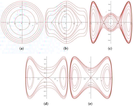
Figure 1.
The bifurcations of the phase trajectories of System (18) with . (a) ; (b) ; (c) ; (d) ; (e) .
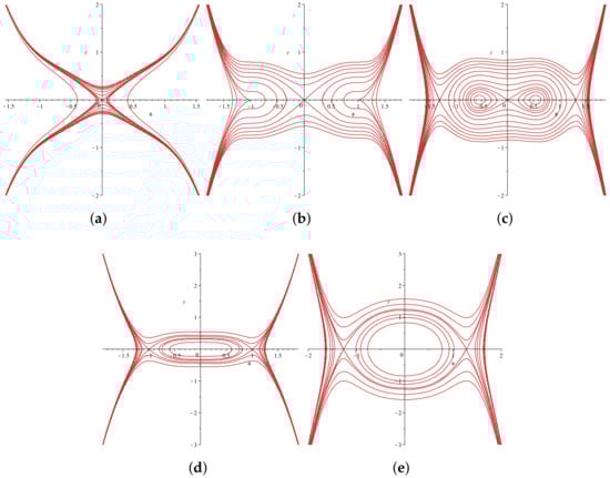
Figure 2.
The bifurcations of the phase trajectories of System (18) with . (a) ; (b) ; (c) ; (d) ; (e) .
2.2. The Case of
When , System (15) becomes
And its first integral is
Now, we have . Denote that and , where . Through the discussion to the zero points of the function , we obtain the same conclusion as the number of equilibria in Section 2.1, with the sole distinction that the equilibrium point O remains degenerate throughout. In this case, the number and qualitative properties of equilibria in System (20) are listed in Table 3 and Table 4, and the phase trajectories of System (20) is shown in Figure 3 and Figure 4.
Table 3.
Number and qualitative properties of equilibria in System (20) for or , .
Table 4.
Number and qualitative properties of equilibria in System (20) for or , .
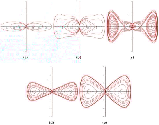
Figure 3.
The bifurcations of the phase trajectories of System (20) with . (a) , , ; (b) , , ; (c) , , ; (d) , , ; (e) , , .
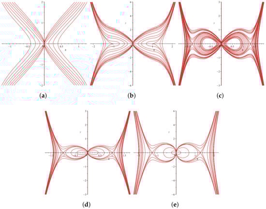
Figure 4.
The bifurcations of the phase trajectories of System (20) with . (a) , , ; (b) , , ; (c) , , ; (d) , , ; (e) , , .
For , we have the following:
For , these can be similarly discussed.
2.3. The Case of
When , System (15) becomes
And its first integral is
Similarly to , we obtain the same conclusion as the case of relative to the number and qualitative properties of equilibria, and the phase trajectories of System (22) is given in Figure 5 and Figure 6.
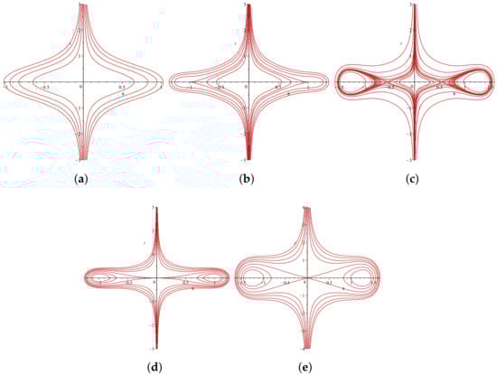
Figure 5.
The bifurcations of the phase trajectories of System (22) with . (a) , ; (b) , , ; (c) , , ; (d) , , ; (e) , , .
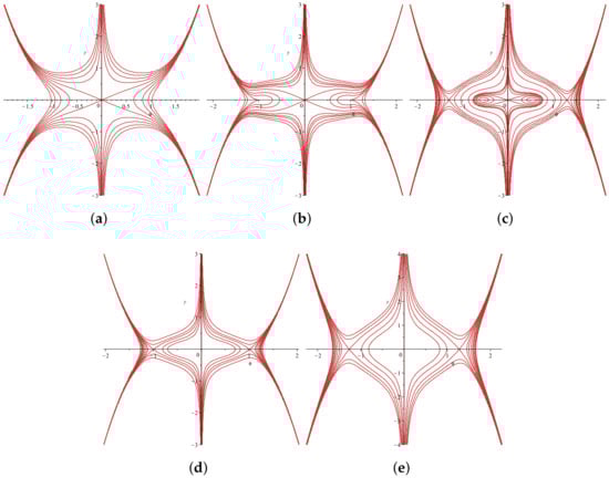
Figure 6.
The bifurcations of the phase trajectories of System (22) with . (a) , , ; (b) , , ; (c) , , ; (d) , , ; (e) , , .
3. Bifurcations of the Phase Trajectories of System (11)
We first consider all possible trajectories of System (11). Then, we obtain the associated regular system of (11) as follows:
In the following, we denote that . Then, its derivative is . It is obvious that the equilibrium points of System (24) satisfy . Let be the coefficient matrix of the linearized system of (24) at the equilibrium point . We have
We will discuss all possible phase trajectories of System (24) for and in this section. In this case, System (24) can be reduced to
Now, we have . Denote that and , where . Through the discussion to the zero points of the function , we obtain the following conclusions.
For , we have the following:
For , these can be similarly discussed.
Employing planar dynamical systems theory, Table 5 and Table 6 comprehensively characterize both the quantity and qualitative nature of equilibrium points for System (25). Furthermore, Figure 7 and Figure 8 present the corresponding phase-trajectory analysis of the system’s dynamical behavior.
Table 5.
Number and qualitative properties of equilibria in System (25) for .
Table 6.
Number and qualitative properties of equilibria in System (25) for .
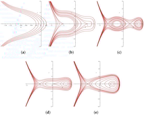
Figure 7.
The bifurcations of the phase trajectories of System (25) with . (a) , , ; (b) , , ; (c) , , ; (d) , , ; (e) , , .
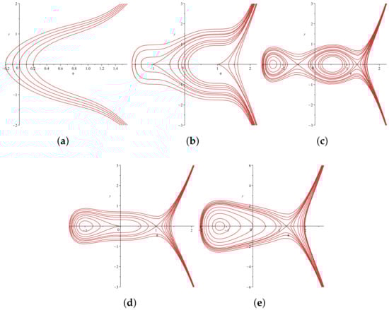
Figure 8.
The bifurcations of the phase trajectories of System (25) with . (a) , , ; (b) , , ; (c) , ; (d) , , ; (e) , .
4. Bifurcations of Phase Trajectories of System (13)
We first consider all possible trajectories of System (13). Then, we obtain the associated regular system of (13) as follows:
In the following, we denote that . Then, its derivative is . It is obvious that the equilibrium points of System (27) satisfy . Let be the coefficient matrix of the linearized system of (27) at the equilibrium point . We have
We will discuss all possible phase trajectories of System (27) for and in this section. In this case, System (27) can be reduced to
The first integral of System (28) can be obtained from (14) as follows:
Now, we have . Denote that and , where . Through the discussion to the zero points of the function , we obtain the following conclusions.
For , we have the following:
For , these can be similarly discussed.
Leveraging planar dynamical systems theory, Table 7 and Table 8 delineate the cardinality and qualitative attributes of equilibria in System (28). Complementing this analysis, Figure 9 and Figure 10 illustrate the numerically computed phase trajectories of the system, offering a geometric representation of its dynamical behavior.
Table 7.
Number and qualitative properties of equilibria in System (28) for .
Table 8.
Number and qualitative properties of equilibria in System (28) for .
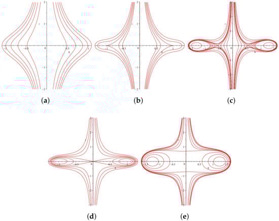
Figure 9.
The bifurcations of the phase trajectories of System (28) with . (a) , , ; (b) , , ; (c) , ; (d) , , ; (e) , , .
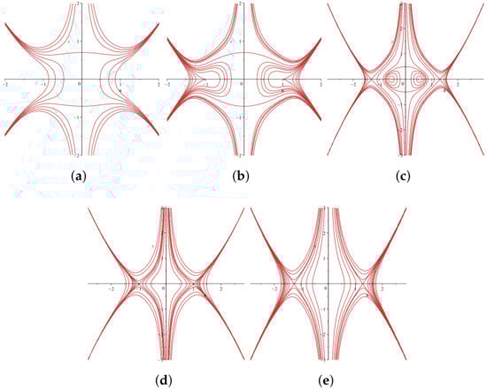
Figure 10.
The bifurcations of the phase trajectories of System (28) with . (a) , , ; (b) , , ; (c) , ; (d) , , ; (e) , , .
5. Exact Explicit Solutions for
In this section, we calculate the possible exact explicit parametric representations of the orbits given by Figure 1, Figure 2, Figure 3, Figure 4, Figure 5 and Figure 6 for different parametric conditions.
5.1. The Case of
The exact explicit parametric representations of the phase orbits depicted in Figure 1 and Figure 2 are derivable directly from Equation (30). For the convenience of later expressions, we denote and , where ().
5.1.1. The Subcase of , , and
(I) For , corresponding to the closed-orbit families defined by , , in Figure 1a, (30) can be written as
Here, , , and are all the roots of , is the real root, and are complex roots, and , where . We have the following periodic solution family:
where , , , , and . and are Jacobian elliptic functions. Periodic solutions in the context of traveling waves signify stable, oscillatory waveforms where energy is uniformly distributed across each oscillation cycle. A prime example of such phenomena is optical frequency combs, which consist of a series of evenly spaced, stable optical frequencies. These periodic traveling-wave solutions embody a state of equilibrium where the effects of dispersion play a dominant role, carefully balancing out other factors in the wave-propagation process. This balance ensures the persistence and stability of the oscillatory pattern over time and space.
(II) For , corresponding to the closed-orbit families defined by , , in Figure 1b, (30) can be written as
Here, , , and are all the roots of , is the real root, and are complex roots, and , where . Then, we can obtain the same expression as (31).
(III) The case of .
Here , , , and are all real roots of and . We have the following periodic solution family:
where and .
(ii) Corresponding to the closed-orbit families defined by and , in Figure 1c, (30) can be written as
Here, , , and are all real roots of and , where . We have the following periodic solution family:
where and .
Here, and . We have the following solution family:
where . As a special solution connecting two different equilibrium states, the heteroclinic traveling-wave solution can reveal key dynamical characteristics in optical fiber nonlinear systems, such as the propagation speed of waves, waveform changes, and energy conversion.
(iv) Corresponding to the global closed-orbit families defined by and , in Figure 1c, (30) can be written as
Here, , , and are all roots of ; is the real root; and are complex roots; , where . Then, we can obtain the same expression as (31).
(IV) For the case of .
Here, and . We have the following periodic solution family:
where .
(ii) Corresponding to the closed-orbit families defined by and , in Figure 1d, (30) can be written as
Here, , , and are all roots of ; is the real root; and are complex roots; , where . Then, we can obtain the same expression as (31).
(V) For , corresponding to the closed-orbit families defined by and , in Figure 1e, (30) can be written as
Here, , , and are all roots of ; is the real root; and are complex roots; , where . Then, we can obtain the same expression as (31).
5.1.2. The Subcase of , , and
(I) For the case of .
(i) Corresponding to the closed-orbit families defined by , , in Figure 2c, (30) can be written as
Here, , , and are all real roots of , and , where . We have the following periodic solution family:
where and .
(ii) Corresponding to the right homoclinic orbit defined by , in Figure 2c, (30) can be written as
Here, , , and are all real roots of , and , where . We have the following periodic solution family:
where and .
Homoclinic solutions offer a mathematical depiction of localized solitary waves that exist in physical systems. These solitary waves, such as optical solitons that maintain their shape and speed over long distances in optical fibers due to a delicate balance between nonlinear and dispersive effects or neural spikes that are brief, intense electrical impulses in neurons, are fundamentally governed by nonlinear self-trapping effects. This self-trapping phenomenon arises from the interplay of nonlinear forces within the system, which confine the wave’s energy to a relatively small spatial region, allowing it to propagate as a distinct self-sustained entity.
5.2. The Case of
The exact explicit parametric representations of the phase orbits depicted in Figure 3 and Figure 4 are derivable directly from Equation (38).
5.2.1. The Subcase of , , and
(I) For , corresponding to the closed-orbit families defined by , in Figure 3c, (38) can be written as
Here, , , , and are all real roots of , and . We have the following periodic solution family:
where and .
5.2.2. The Subcase of , , and
(I) For , corresponding to the closed-orbit families defined by , in Figure 4c, (38) can be written as
Here, , , and are all real roots of , and , where . We have the following periodic solution family:
where , and .
5.3. The Case of
The exact explicit parametric representations of the phase orbits depicted in Figure 5 and Figure 6 are derivable directly from Equation (42).
5.3.1. The Subcase of , , and
(I) For , corresponding to the closed-orbit families defined by , in Figure 5c, (42) can be written as
Here, , , , and are all real roots of , and . We have the following periodic solution family:
where , and .
5.3.2. The Subcase of , , and
6. Exact Explicit Solutions for
The exact explicit parametric representations of the phase orbits depicted in Figure 7 and Figure 8 are derivable directly from Equation (46).
6.1. The Case of , , and
(I) For , corresponding to the closed-orbit families defined by , in Figure 7d, (46) can be written as
We have the following periodic solution family:
where and .
6.2. The Case of , , and
(I) For , corresponding to the closed-orbit families defined by , in Figure 8d, (46) can be written as
We have the following periodic solution family:
where , .
7. Exact Explicit Solutions for
The exact explicit parametric representations of the phase orbits depicted in Figure 9 and Figure 10 are derivable directly from Equation (49).
7.1. The Case of , , and
(I) For , corresponding to the closed-orbit families defined by , in Figure 9c, (49) can be written as
Here, and are all real roots of , and . We have the following periodic solution family:
where , .
(II) For , corresponding to the closed-orbit families defined by , in Figure 9d, (49) can be written as
Here, . We have the following periodic solution family:
where .
(III) For , corresponding to the closed-orbit families defined by , in Figure 9e, (49) can be written as
Here, is the real root, and denotes complex roots. We have the following periodic solution family:
where .
7.2. The Case of , , and
(I) For , corresponding to the closed-orbit families defined by , in Figure 10c, (49) can be written as
Here, and are all real roots of , and . We have the following periodic solution family:
where , .
8. Conclusions
The nonlinear Schrödinger equation with Kudryashov’s quintic power law of the refractive index together with the dual form of nonlocal nonlinearity is studied in this paper using the method of dynamical systems. Our analysis focused on three specific parameter regimes where : (i) ; (ii) ; and (iii) . Through phase-space analysis and first-integral techniques, we successfully derived exact periodic wave solutions, along with homoclinic and heteroclinic solutions, corresponding to different topological structures in the phase-trajectory plot.
The current work intentionally restricts consideration to these parameter configurations due to their mathematical tractability. For more general cases where the integrand function becomes overly complex, obtaining closed-form solutions remains challenging with standard dynamical system approaches. Therefore, there is a necessity for the development of more advanced analytical or semi-analytical methods that can effectively manage higher-dimensional parameter spaces and non-integrable scenarios. There is a necessity for the development of more sophisticated analytical or semi-analytical methods that can effectively manage higher-dimensional parameter spaces and non-integrable scenarios. This will enable us to extend our analysis to a broader range of parameter conditions. Additionally, further exploration of generalized models that incorporate additional nonlinear terms or different forms of nonlocal nonlinearity is required. This will help in understanding the universal behaviors and specific characteristics of nonlinear Schrödinger equations in various physical contexts.
In conclusion, our study provides a significant step forward in understanding the solutions of the nonlinear Schrödinger equation with Kudryashov’s quintic power law and dual nonlocal nonlinearity. The exact solutions obtained offer valuable insights, while the identified challenges and future research directions set the stage for further advancements in the field.
Author Contributions
C.C.: Conceptualization, methodology, writing—original draft preparation, and software and editing; M.Y.: software, resources, and editing; Q.Z.: conceptualization, methodology, writing—review and editing, and supervision. All authors have read and agreed to the published version of this manuscript.
Funding
This work was supported by the National Natural Science Foundation of China (12101090); Sichuan Natural Science Foundation (2023NSFSC0071 and 2023NSFSC1362); Sichuan Province Science and Technology Support Program (2023ZYD0001); Chengdu University of Information Technology Science and Technology Innovation Capability Enhancement Plan Innovation Team Key Project (KYTD202322); and the Talent Introduction Program of Chengdu University of Information Technology (KYTZ202185).
Data Availability Statement
No data were used to support this study.
Conflicts of Interest
The authors declare no conflicts of interest.
References
- Radhakrishnan, R.; Kundu, A.; Lakshmanan, M. Coupled nonlinear Schrödinger equations with cubic-quintic nonlinearity: Integrability and soliton interaction in non-Kerr media. Phys. Rev. E 1999, 60, 3314. [Google Scholar] [CrossRef]
- Zheng, C. Exact nonreflecting boundary conditions for one-dimensional cubic nonlinear Schrödinger equations. J. Comput. Phys. 2006, 215, 552–565. [Google Scholar] [CrossRef]
- Wazwaz, A.M. Exact solutions for the fourth order nonlinear Schrodinger equations with cubic and power law nonlinearities. Math. Comput. Model. 2006, 43, 802–808. [Google Scholar] [CrossRef]
- Zhang, L.; Chen, L.Q. Envelope compacton and solitary pattern solutions of a generalized nonlinear Schrödinger equation. Nonlinear Anal. Theory Methods Appl. 2009, 70, 492–496. [Google Scholar] [CrossRef]
- Guo, C.; Guo, B. The existence of global solutions for the fourth-order nonlinear Schrödinger equations. J. Appl. Anal. Comput. 2019, 9, 1183–1192. [Google Scholar] [CrossRef]
- Zhang, Q.; Zhou, Y.; Li, J. Bifurcations and exact solutions of the nonlinear Schrödinger equation with nonlinear dispersion. Int. J. Bifurc. Chaos 2022, 32, 2250041. [Google Scholar] [CrossRef]
- Ekici, M. Optical solitons with Kudryashov’s quintuple power-law nonlinearity coupled with dual form of generalized non-local refractive index structure. Optik 2021, 243, 166723. [Google Scholar]
- Kudryashov, N.A. Model of propagation pulses in an optical fiber with a new law of refractive indices. Optik 2021, 248, 168160. [Google Scholar] [CrossRef]
- Ekici, M. Optical solitons with Kudryashov’s quintuple power–law coupled with dual form of non–local law of refractive index with extended Jacobi’s elliptic function. Opt. Quantum Electron. 2022, 54, 279. [Google Scholar] [CrossRef]
- Eldidamony, H.A.; Ahmed, H.M.; Zaghrout, A.S.; Ali, Y.S.; Arnous, A.H. Optical solitons with Kudryashov’s quintuple power law nonlinearity having nonlinear chromatic dispersion using modified extended direct algebraic method. Optik 2022, 262, 169235. [Google Scholar] [CrossRef]
- Samir, I.; Arnous, A.H.; Yıldırım, Y.; Biswas, A.; Moraru, L.; Moldovanu, S. Optical solitons with cubic-quintic-septic-nonic nonlinearities and quadrupled power-law nonlinearity: An observation. Mathematics 2022, 10, 4085. [Google Scholar] [CrossRef]
- Li, R.; Sinnah, Z.A.B.; Shatouri, Z.M.; Manafian, J.; Aghdaei, M.F.; Kadi, A. Different forms of optical soliton solutions to the Kudryashov’s quintuple self-phase modulation with dual-form of generalized nonlocal nonlinearity. Results Phys. 2023, 46, 106293. [Google Scholar] [CrossRef]
- Shakeel, M.; Bibi, A.; Chou, D.; Zafar, A. Study of optical solitons for Kudryashov’s Quintuple power-law with dual form of nonlinearity using two modified techniques. Optik 2023, 273, 170364. [Google Scholar] [CrossRef]
- Rabie, W.B.; Ahmed, H.M. Constructing new soliton solutions for Kudryashov’s quintuple self-phase modulation with dual-form of generalized nonlocal nonlinearity using extended f-expansion method. Opt. Quantum Electron. 2023, 55, 233. [Google Scholar] [CrossRef]
- Ali, K.K.; Mehanna, M.S.; Mohamed, M.S. Optical soliton solutions for Kudryashov’s quintuple power-law coupled with dual form of non-local refractive index. Opt. Quantum Electron. 2023, 55, 1255. [Google Scholar] [CrossRef]
- Zayed, E.M.E.; El-Shater, M.; Arnous, A.H.; Yıldırım, Y.; Hussein, L.; Jawad, A.J.M.; Veni, S.S.; Biswas, A. Quiescent optical solitons with Kudryashov’s generalized quintuple-power law and nonlocal nonlinearity having nonlinear chromatic dispersion with generalized temporal evolution by enhanced direct algebraic method and sub-ODE approach. Eur. Phys. J. Plus 2024, 139, 885. [Google Scholar] [CrossRef]
- Ashraf, M.A.; Seadawy, A.R.; Rizvi, S.T.R.; Althobaiti, A. Dynamical optical soliton solutions and behavior for the nonlinear Schrödinger equation with Kudryashov’s quintuple power law of refractive index together with the dual-form of nonlocal nonlinearity. Opt. Quantum Electron. 2024, 56, 1243. [Google Scholar] [CrossRef]
- Murad, M.A.S. Optical solutions with Kudryashov’s arbitrary type of generalized non-local nonlinearity and refractive index via the new Kudryashov approach. Opt. Quantum Electron. 2024, 56, 999. [Google Scholar] [CrossRef]
- Li, J. Singular Nonlinear Traveling Wave Equations: Bifurcation and Exact Solutions; Science: Beijing, China, 2013. [Google Scholar]
- Li, J.; Chen, G. On a class of singular nonlinear traveling wave equations. Int. J. Bifurc. Chaos 2007, 17, 4049–4065. [Google Scholar] [CrossRef]
- Yu, M.; Chen, C.; Zhang, Q. Bifurcations and exact solutions of the generalized Radhakrishnan–Kundu–Lakshmanan equation with the polynomial law. Mathematics 2023, 11, 4351. [Google Scholar] [CrossRef]
- Li, J.; Dai, Y. Bifurcations and Exact Traveling Wave Solutions for the Model of Slightly Dispersive Quasi-Incompressible Hyperelastic Materials. Qual. Theory Dyn. Syst. 2025, 24, 10. [Google Scholar] [CrossRef]
Disclaimer/Publisher’s Note: The statements, opinions and data contained in all publications are solely those of the individual author(s) and contributor(s) and not of MDPI and/or the editor(s). MDPI and/or the editor(s) disclaim responsibility for any injury to people or property resulting from any ideas, methods, instructions or products referred to in the content. |
© 2025 by the authors. Licensee MDPI, Basel, Switzerland. This article is an open access article distributed under the terms and conditions of the Creative Commons Attribution (CC BY) license (https://creativecommons.org/licenses/by/4.0/).