Article

Fast Implementation of Generalized Koebe’s Iterative Method

1
Department of Mathematical Sciences, Faculty of Science, Universiti Teknologi Malaysia (UTM), Johor Bahru 81310, Johor, Malaysia
2
Department of Mathematics, Statistics & Physics, Wichita State University, Wichita, KS 67260-0033, USA
*
Author to whom correspondence should be addressed.
Mathematics 2025, 13(12), 1920; https://doi.org/10.3390/math13121920
Submission received: 11 April 2025 / Revised: 31 May 2025 / Accepted: 5 June 2025 / Published: 9 June 2025

Abstract

Let G be a given bounded multiply connected domain of connectivity m + 1 bounded by smooth Jordan curves. Koebe’s iterative method is a classical method for computing the conformal mapping from the domain G onto a bounded multiply connected circular domain obtained by removing m disks from the unit disk. Koebe’s method has been generalized to compute the conformal mapping from the domain G onto a bounded multiply connected circular domain obtained by removing m 1 disks from a circular ring. A fast numerical implementation of the generalized Koebe’s iterative method is presented in this paper. The proposed method is based on using the boundary integral equation with the generalized Neumann kernel. Several numerical examples are presented to demonstrate the accuracy and efficiency of the proposed method.

1. Introduction

In the study of conformal mappings of multiply connected domains in the extended complex plane C { } , a variety of canonical domains onto which a given domain can be mapped have been extensively investigated in the literature (see [1,2,3] for details). Most of these canonical domains are slit domains; see [4,5]. Conformal mappings onto slit domains are closely connected to several fundamental concepts in potential theory, including Green’s functions, modified Green’s functions, and harmonic measures [1,2], and also play a significant role in addressing various problems in applied mathematics [1,6]. Several numerical methods for computing conformal mappings onto slit domains have been proposed in the literature. For example, a unified method has been presented in [7,8,9] for computing conformal mappings onto the thirty-nine canonical slit domains cataloged by Koebe in [4] and has been extended in [10] to compute conformal mappings onto the canonical domain obtained by removing m rectilinear slits from an infinite strip [5]. The method relies on using the boundary integral equation with the generalized Neumann kernel.
An important canonical multiply connected domain that is not a slit domain is the circular domain, i.e., a domain all of whose boundary components are circles (see [3,11,12]). Circular domains are ideal for using Fourier series and FFT [13,14]. Further, analytic formulas exist for several applied problems in circular domains (see the recent monograph [1] and the references cited therein). See also [15]. Koebe’s iterative method [3] is the first numerical method for computing conformal mappings onto circular domains. Several numerical implementations of Koebe’s iterative method have been proposed in the literature; see [12,15,16,17,18,19,20] for details. The fast and accurate method presented in [18,19] is based on a combination of the usage of the boundary integral equation with the generalized Neumann kernel and the fast multipole method (FMM). For numerical methods for computing conformal mappings from circular domains onto multiply connected domains, see [13,21].
A special class of the canonical bounded circular domains is the circular ring with circular holes domain. The circular domain computed by the classical Koebe’s iterative method mentioned above is not necessarily a circular ring with circular holes. Zeng et al. [22] have developed a generalization of Koebe’s iterative method to compute conformal mappings from bounded multiply connected domains onto a circular ring with a circular hole domain. The classical Koebe’s method transforms one boundary component into a circle at each iteration, while the generalized Koebe’s method simultaneously maps two boundary components onto two concentric circles. From the measurement of the roundness of the boundary components, the generalized Koebe’s method converges much faster than the classical Koebe’s method. The generalized Koebe’s method was implemented in [22] using the discrete Yamabe flow method. The aim of this paper is to introduce a new, fast, and accurate numerical implementation of the generalized Koebe’s iterative method. The proposed approach utilizes the boundary integral equation with the Neumann kernel, combined with the fast multipole method (FMM). This method yields the boundary values of both the conformal mapping and its derivative. The values of the mapping function as well as its inverse for interior points can then be calculated using the Cauchy integral formula. The proposed method is applicable to domains with very high connectivity, domains with piecewise smooth boundaries, and domains with close-to-touching boundary components. Similar to the implementation of the classical Koebe’s method described in [18,19], the computational complexity of the proposed method for computing conformal mappings from bounded multiply connected domains of connectivity m + 1 on a circular ring with m 1 circular holes is also O m n ( m + log n ) , where n is the number of collocation points in the discretization of each boundary component.
This paper has the following structure. The conformal mapping from bounded multiply connected domains onto circular ring with circular holes domains is introduced in Section 2. Section 3 and Section 4 introduce fast numerical methods for computing the conformal mapping from unbounded simply connected domains onto the unit disk and from unbounded doubly connected domains onto a circular ring, respectively. A fast numerical implementation of the generalized Koebe’s iterative method is introduced in Section 5. In Section 6, we provide five numerical examples to demonstrate the effectiveness of the proposed method. Final remarks and conclusions are presented in Section 7.

2. The Circular Ring with Circular Holes Map

Consider a bounded multiply connected domain G of connectivity m + 1 with Γ = G = k = 0 m Γ k where Γ 0 , Γ 1 , , Γ m are smooth Jordan curves such that Γ 0 encloses all the other curves Γ 1 , , Γ m . The orientation of the outer curve Γ 0 is counterclockwise, while the orientations of the inner curves Γ 1 , Γ 2 , , Γ m are clockwise so that G is always on the left of Γ . Then, there exists a conformal mapping w = ω ( z ) from the domain G onto a circular domain Ω obtained by removing m disks from the unit disk. The boundary C = k = 0 m C k of Ω consists of m + 1 circles C 0 , C 1 , , C m where the circle C k is the image of the curve Γ k , k = 0 , 1 , , m , and the circle C 0 encloses all the other circles. Such a conformal mapping w = ω ( z ) is not unique. If we assume that the external circle C 0 is the unit circle, then the mapping w = ω ( z ) is unique up to a Möbius transformation. Thus, the mapping w = ω ( z ) can be made uniquely determined by fixing three real parameters [21,23]. One way to fix these three parameters is by assuming that w = ω ( z ) maps three given points of the outer boundary Γ 0 ordered in counterclockwise orientation onto three points on the unit circle with the same orientation. We can also fix the three real parameters by assuming that ω ( α ) = 0 and ω ( α ) > 0 , where α is a given point in G. Another way of fixing these three parameters is by locating the center of the circle C 1 at the origin and by assuming that ω ( α ) > 0 for the given point α in G. In the latter case, the canonical domain Ω is a circular ring with m 1 circular holes (see Figure 1). Finding such a canonical domain Ω and computing the unique conformal mapping w = ω ( z ) from G onto Ω is the topic of this paper. We assume w = ω ( z ) maps the curve Γ 0 onto the unit circle C 0 : | w | = R 0 = 1 , the curve Γ 1 onto the circle C 1 : | w | = R 1 , and the curves Γ k , k = 2 , , m , onto the circles C k : | w z k | = R k , where z k and R k are the center and the radius of the circle C k , respectively. The centers z 2 , z 3 , , z m and the radii R 1 , R 2 , , R m are unknown and must be determined.
For the given bounded multiply connected domain G, both the classical and the generalized Koebe’s iterative methods can be used to compute conformal mappings from the domain G onto circular domains. Each iteration of the classical Koebe’s method involves computing the conformal mapping of m unbounded simply connected domains onto the exterior of the unit disk, as well as computing a conformal mapping of one bounded simply connected domain onto the unit disk. The successive computed domain gradually approaches a circular domain. During the process, we compute approximate values for the unknown centers and radii of the circles [3,12,18,19]. For the proof of convergence and the converging rate for the classical Koebe’s method, see [3]. The circular domain obtained using the classical Koebe’s method is not necessarily a circular ring with circular holes domain. Conformal mappings from the bounded multiply connected domain G onto a circular ring with m 1 circular holes domain can be computed using a generalization of Koebe’s method as proposed in [22]. For odd m, each iteration of the generalized Koebe’s method requires ( m + 1 ) / 2 times of computing a conformal mapping from an unbounded doubly connected domain onto a circular ring. When m is even, each iteration of the generalized Koebe’s method requires m / 2 times computing a conformal mapping of an unbounded doubly connected domain onto a circular ring and also computing a conformal mapping from an unbounded simply connected domain onto the unit disk. The successive computed domains approach gradually forms a circular ring with m 1 circular holes in the domain (see [22] and Figure 2 and Figure 3 below). In the process, we compute approximate values of the unknown centers and radii of the circles. The proof of convergence of the generalized Koebe’s iterative method is given in [22].

3. Conformal Mappings from Unbounded Simply Connected Domains onto the Unit Disk

Let S be an unbounded simply connected domain in the extended complex plane C { } such that S and S = L . We assume that z 1 is a given point in the interior of L. The orientation of L is assumed to be such that S is on the left of L, i.e., L is oriented clockwise. We parametrize the curve L by a 2 π -periodic twice continuously differentiable complex function η ( t ) with non-vanishing first derivative η ( t ) 0 for t J = [ 0 , 2 π ] . With the parametrization η ( t ) , we define the Neumann kernel on J × J by [3,24]
N ( s , t ) = 1 π Im η ( t ) η ( t ) η ( s ) .
The kernel N ( s , t ) is continuous with
N ( t , t ) = 1 2 π Im η ( t ) η ( t ) .
We define also the kernel [24]
M ( s , t ) = 1 π Re η ( t ) η ( t ) η ( s ) ,
which can be written as
M ( s , t ) = 1 2 π cot s t 2 + M 1 ( s , t )
with a continuous kernel M 1 ( s , t ) that takes on the diagonal the values
M 1 ( t , t ) = 1 2 π Re η ( t ) η ( t ) .
Thus, the integral operator
N μ ( s ) = J N ( s , t ) μ ( t ) d t , s [ 0 , 2 π ] ,
is a Fredholm integral operator and the operator
M μ ( s ) = J M ( s , t ) μ ( t ) d t , s [ 0 , 2 π ] ,
is a singular integral operator since the kernel M ( s , t ) is singular.
In this section, we review a numerical method for computing the conformal mapping w = Φ ( z ) from the unbounded simply connected domain S onto the unit disk D = { w : | w | < 1 } from ([7], §4.2) and [25]. With the normalization
Φ ( ) = 0 , Φ ( ) = lim z ( z Φ ( z ) ) > 0 ,
the conformal mapping Φ is unique. The mapping function w = Φ ( z ) is assumed to map the curve L onto the unit circle. It can be expressed in the form
Φ ( z ) = c z z 1 e f ( z ) ,
where c = Φ ( ) > 0 is an undetermined real constant and z 1 is a given point in the exterior of S. The boundary values of the function f ( z ) are given by
f ( η ( t ) ) = γ ( t ) + h ( t ) + i μ ( t ) , t J ,
where
γ ( t ) = log η ( t ) z 1
and h ( t ) is a constant function with h ( t ) = log c . The function μ is the unique solution to the integral equation with the Neumann kernel
( I N ) μ = M γ
and the constant function h is given by
h = [ M μ ( I N ) γ ] / 2 .
It is known (for unbounded simply or multiply connected domains) that λ = 1 is not an eigenvalue of the operator N (see [26] [Theorem 8]). All eigenvalues of N are real and lie in the interval [ 1 , 1 ) , which implies that all eigenvalues of the operator I N are in the interval ( 0 , 2 ] . Thus, by the Fredholm alternative theorem [27], the operator I N is invertible and its inverse is bounded. In the numerical experiments presented in this paper, the integral Equation (10) is solved using the MATLAB function fbie described in [25]. This function applies the Nyström method with the trapezoidal rule to discretize the integral Equation (10) using n equidistant collocation points, defined by
t k = ( k 1 ) 2 π n , k = 1 , 2 , , n ,
resulting in an n × n linear system. This system is solved using the MATLAB function gmres, where the matrix-vector product in the function gmres is computed in O ( n ) operations using the MATLAB function zfmm2dpart from the FMMLIB2D toolbox developed by Greengard and Gimbutas [28]. The total computational cost of the method is then O ( n log n ) operations [18,25]. In the function zfmm2dpart, the parameter iprec is set to 5, corresponding to an FMM tolerance of 0.5 × 10 15 . For the solver gmres, we set the parameters restart=[], gmrestol=1e-14, and maxit=100, which means that the GMRES method runs without restarting, with a tolerance of 10 14 and a maximum of 100 outer iterations.
By solving the integral Equation (10) for μ and by computing the constant h through (11), we obtain the boundary values of f through (9) and the constant c by c = e h . For z S , the values of the analytic function f ( z ) can be computed by the Cauchy integral formula.
f ( z ) = 1 2 π i L f ( η ) η z d η .
A MATLAB function fcau for accurate computation of f ( z ) can be downloaded from https://github.com/mmsnasser/plgcirmap (accessed on 1 June 2025). This function computes the values of the function f ( z ) accurately even when z is close to the boundary of the domain; see [25] for details. Then the values of the conformal mapping w = Φ ( z ) from the unbounded simply connected domain S onto the unit disk D can be computed for z S L through (8).

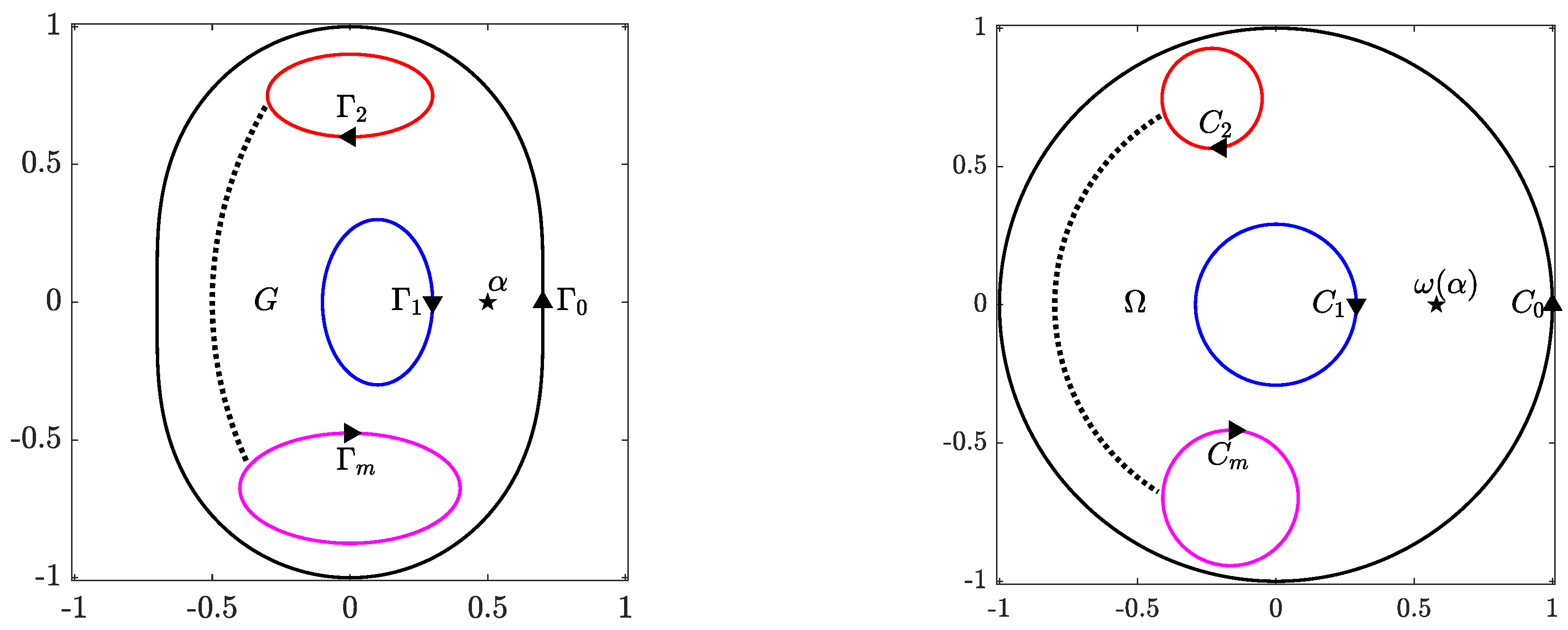
4. Conformal Mappings from Unbounded Doubly Connected Domains onto a Circular Ring

In this section, we review a method from ([7], §4.1) that extends the method presented in the previous section to doubly connected domains. Let S be an unbounded doubly connected domain in the extended complex plane C { } such that S and S = L = L 1 L 2 . We assume that z 1 is a given point in the interior of L 1 and z 2 is a given point in the interior of L 2 . Both curves L 1 and L 2 are assumed to be oriented clockwise. Each curve L j , j = 1 , 2 , is parametrized by a 2 π -periodic twice continuously differentiable complex function η j ( t ) with non-vanishing first derivative η j ( t ) 0 for t J j = [ 0 , 2 π ] . We define the total parameter domain J as the disjoint union of the two intervals J 1 and J 2 . Then, the whole boundary L is parametrized by the complex function η ( t ) defined on J by
η ( t ) = η 1 ( t ) , t J 1 = [ 0 , 2 π ] , η 2 ( t ) , t J 2 = [ 0 , 2 π ] .
Let w = Ψ ( z ) be a conformal mapping from the unbounded doubly connected domain S onto the annulus R = { w : R < | w | < 1 } , where R is an undetermined real constant. With the normalization Ψ ( ) > 0 , the conformal mapping Ψ is unique. The mapping function w = Ψ ( z ) is assumed to map the curve L 1 onto the unit circle and the curve L 2 onto the circle | w | = R . The mapping function w = Ψ ( z ) can be expressed in the form [7]
Ψ ( z ) = c z z 2 z z 1 e f ( z ) ,
where c = Ψ ( ) > 0 is an undetermined real constant, z 1 is a given point in the interior of L 1 , and z 2 is a given point in the interior of L 2 .
With the parametrization η ( t ) in (13), let the Neumann kernel N ( s , t ) and the kernel M ( s , t ) be defined on J × J as in (1) and (3). Let also the integral operators N and M be defined as in (6) and (7). Then the boundary values of the function f ( z ) in (14) are given by (9), where [7]
γ ( t ) = log η ( t ) z 1 η ( t ) z 2
and h ( t ) is the piecewise constant function
h ( t ) = h 1 , t J 1 = [ 0 , 2 π ] , h 2 , t J 2 = [ 0 , 2 π ] ,
with h 1 = log c and h 2 = log R log c . The function μ is the unique solution to the integral Equation (10), and the piecewise constant h is given by (11). For the doubly connected domain S, the integral Equation (10) will be solved also by the MATLAB function fbie, and the computational cost of the method is O ( n log n ) operations [25]. By solving the integral Equation (10) for μ and by computing the h through (11), we obtain the boundary values of f through (9). We also obtain the value of the constants c and R from the piecewise constant function h by c = e h 1 and R = e h 2 h 1 . Then the values of the mapping function w = Ψ ( z ) can be computed for z S L through (14), where the values of the analytic function f ( z ) can be computed for z S by the Cauchy integral formula.

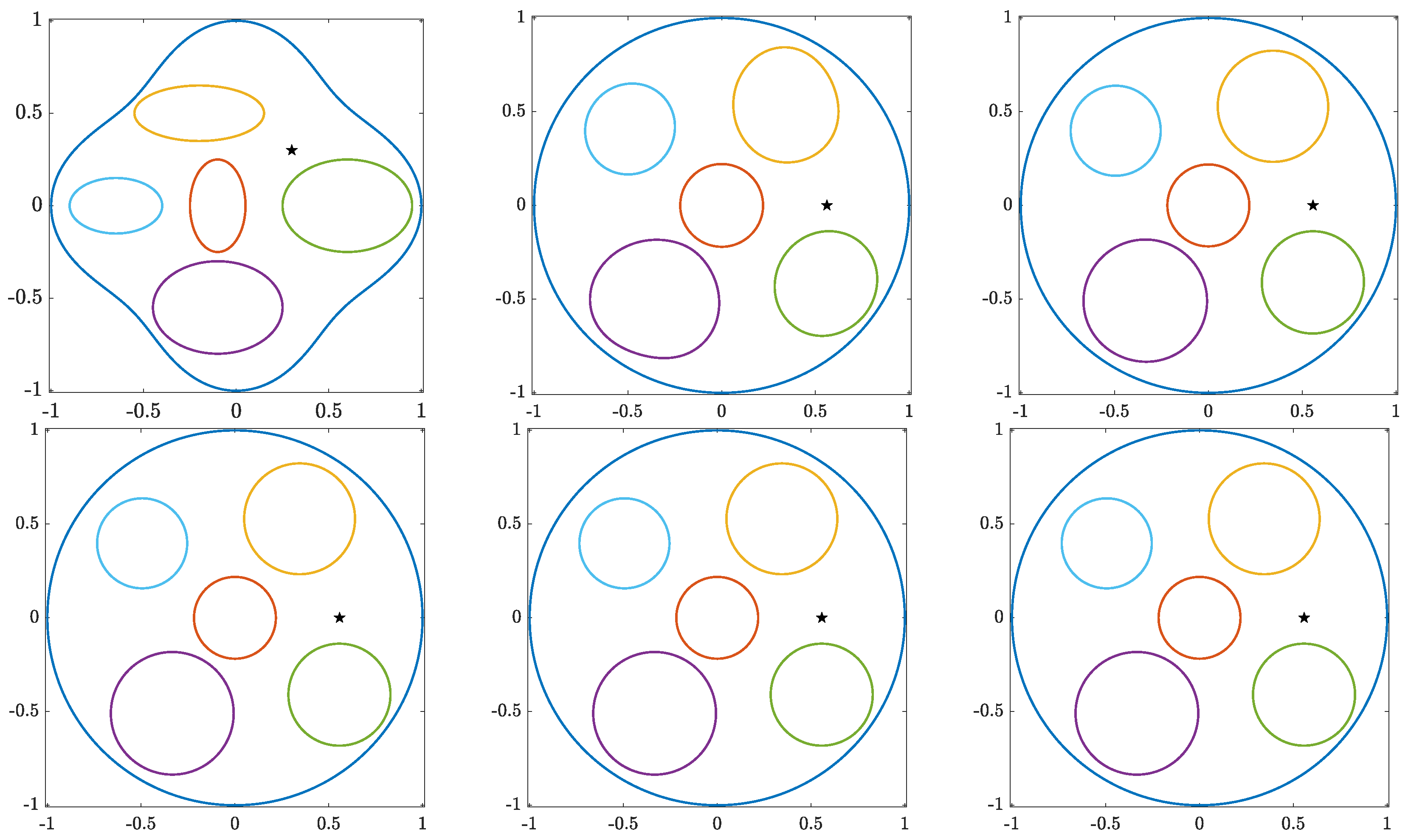
5. Generalized Koebe’s Iterative Method

Let G be a given bounded multiply connected domain such that Γ = G = j = 0 m Γ j , where Γ 0 , Γ 1 , , Γ m are closed smooth Jordan curves. The outer curve Γ 0 is oriented counterclockwise and encloses all the other curves Γ 1 , , Γ m are oriented clockwise. For j = 0 , 1 , , m , the curve Γ j is parametrized by a 2 π -periodic twice continuously differentiable complex function ζ j ( t ) with non-vanishing first derivative ζ j ( t ) 0 for t J j = [ 0 , 2 π ] . The total parameter domain J is the disjoint union of the m + 1 intervals J 0 , J 1 , , J m . Define a parametrization ζ ( t ) of the whole boundary Γ on J by
ζ ( t ) = ζ 0 ( t ) , t J 0 = [ 0 , 2 π ] , ζ 1 ( t ) , t J 1 = [ 0 , 2 π ] , ζ m ( t ) , t J m = [ 0 , 2 π ] .
In this section, based on the methods discussed in the previous two sections, we present a numerical implementation of generalized Koebe’s method for computing the conformal mapping w = ω ( z ) from the bounded multiply connected domain G onto a circular ring with m 1 circular holes domain Ω . The boundary of Ω consists of m + 1 circles represented by C = k = 0 m C k , where the circle C k is the image of the curve Γ k , k = 0 , 1 , , m . The mapping function w = ω ( z ) maps the curve Γ 0 onto the unit circle C 0 : | w | = 1 , the curve Γ 1 onto the circle C 1 : | w | = R 1 , and the curves Γ k , k = 2 , , m , onto the circles C k : | w z k | = R k , where z k and R k are the center and the radius of the circle C k . Our proposed method will compute approximations of the boundary values of the mapping function w = ω ( z ) and its derivative.
ξ ( t ) = ω ( ζ ( t ) ) , ξ ( t ) = ζ ( t ) ω ( ζ ( t ) ) , t J ,
as well as the unknown parameters R 1 , R 2 , , R m and z 2 , , z m of the domain Ω .

5.1. Initializations

We set
C i 0 , 0 = Γ i , i = 0 , 1 , 2 , , m ,
where C i 0 , 0 is parametrized by
ξ i 0 , 0 ( t ) = ζ i ( t ) , t J i , i = 0 , 1 , 2 , , m ,
and
d d t ξ i 0 , 0 ( t ) = ζ i ( t ) , t J i , i = 0 , 1 , 2 , , m .
Thus
w 0 ( ζ ( t ) ) = ξ 0 0 , 0 ( t ) , t J 0 = [ 0 , 2 π ] , ξ 1 0 , 0 ( t ) , t J 1 = [ 0 , 2 π ] , ξ m 0 , 0 ( t ) , t J m = [ 0 , 2 π ] ,
are initial values of the boundary values of the required conformal map. Let α 0 , 0 = α , z 0 0 , 0 = , and let z i 0 , 0 be a given point in the interior of the curve C i 0 , 0 for i = 1 , 2 , , m . Further, we define m ^ = ( m 1 ) / 2 for odd m and m ^ = m / 2 for even m.

5.2. Iterations

For k = 1 , 2 , 3 , (k is the iteration number), the following two steps are repeated:

5.2.1. Step I

For j = 0 , 1 , , m ^ when m is odd and for j = 1 , , m ^ when m is even, let w = Ψ k , j ( z ) be the conformal mapping from the unbounded doubly connected domain D k , j in the exterior of the two curves C m 1 k 1 , j and C m k 1 , j onto the ring domain R k , j < | w | < 1 . The image of the curve C m 1 k 1 , j is the unit circle | w | = 1 which will be denoted by C 0 k 1 , j + 1 , and the image of the curve C m k 1 , j is the circle | w | = R k , j , which will be denoted by C 1 k 1 , j + 1 . The parametrizations
ξ 0 k 1 , j + 1 ( t ) = Ψ k , j ( ξ m 1 k 1 , j ( t ) ) and ξ 1 k 1 , j + 1 ( t ) = Ψ k , j ( ξ m k 1 , j ( t ) )
of the curves C 0 k 1 , j + 1 and C 1 k 1 , j + 1 , respectively, will be computed using the integral equation method as explained in Section 4.
The curves C 0 k 1 , j , C 1 k 1 , j , , C m 2 k 1 , j are in the doubly connected domain D k , j and hence will be mapped by the mapping function w = Ψ k , j ( z ) onto curves in the ring R k , j < | w | < 1 . We define
C i k 1 , j + 1 = Ψ k , 0 ( C i 2 k 1 , j ) , i = 2 , , m .
For i = 2 , , m , the curve C i k 1 , j + 1 is parametrized by
ξ i k 1 , j + 1 ( t ) = Ψ k , j ( ξ i 2 k 1 , j ( t ) )
which can be computed using the Cauchy integral formula. We set z 0 k 1 , j + 1 = and z 1 k 1 , j + 1 = 0 . Further, we set α k 1 , j + 1 = Ψ k , j ( α k 1 , j ) and z i k 1 , j + 1 = Ψ k , j ( z i 2 k 1 , j ) for i = 2 , , m , which will be computed by the Cauchy integral formula.
When m is even, we assume that w = Ψ k , 0 ( z ) is the conformal mapping from the unbounded simply connected domain D k , 0 in the exterior of the curve C m k 1 , 0 onto the unit disk | w | < 1 , which will be denoted by C 0 k 1 , 1 and parametrized by
ξ 0 k 1 , 1 ( t ) = Ψ k , 0 ( ξ m k 1 , 0 ( t ) ) .
Such a conformal mapping and parametrization can be computed using the method presented in Section 3. The curves C 0 k 1 , 1 , C 1 k 1 , 1 , , C m 1 k 1 , 1 are in the simply connected domain D k , 0 and will be mapped by w = Ψ k , 0 ( z ) onto curves
C i k 1 , 1 = Ψ k , 0 ( C i 1 k 1 , 0 ) , i = 1 , , m ,
in the unit disk. For i = 1 , , m , the curve C i k 1 , 1 is parametrized by
ξ i k 1 , 1 ( t ) = Ψ k , 0 ( ξ i 1 k 1 , 0 ( t ) )
which can be computed by the Cauchy integral formula. For this case, we set z 0 k 1 , 1 = , α k 1 , 1 = Ψ k , 0 ( α k 1 , 0 ) and z i k 1 , 1 = Ψ k , 0 ( z i 1 k 1 , 0 ) for i = 1 , , m , which will be computed by the Cauchy integral formula.
The derivative
d d t ξ i k 1 , j + 1 ( t ) , t J i ,
of the parametrization ξ i k 1 , j + 1 ( t ) will be computed for each i = 0 , 1 , , m by first interpolating the real and imaginary parts of ξ i k 1 , j + 1 ( t ) by trigonometric interpolating polynomials of degree n / 2 and then differentiating the interpolating polynomials. A MATLAB function derfft.m for computing these derivatives based on using FFT can be downloaded from https://github.com/mmsnasser/plgcirmap (accessed on 1 June 2025).
Finally, once we compute the parametrization ξ i k 1 , m ^ + 1 ( t ) , t J i , the points z i k 1 , m ^ + 1 , and the point α k 1 , m ^ + 1 , the computed domain will be rotated to make sure that α k 1 , m ^ + 1 is on the positive real axis by setting
ξ i k 1 , m ^ + 1 ( t ) = exp ( i arg ( α k 1 , m ^ + 1 ) ) ξ i k 1 , m ^ + 1 ( t ) , i = 0 , 1 , , m , z i k 1 , m ^ + 1 = exp ( i arg ( α k 1 , m ^ + 1 ) ) z i k 1 , m ^ + 1 , i = 0 , 1 , , m , α k 1 , m ^ + 1 = exp ( i arg ( α k 1 , m ^ + 1 ) ) α k 1 , m ^ + 1 .

5.2.2. Step II

The boundary values of the approximate conformal map w = ω k ( z ) obtained in the k th iteration are given by
ω k ( ζ ( t ) ) = ξ 0 k 1 , m ^ + 1 ( t ) , t J 0 , ξ 1 k 1 , m ^ + 1 ( t ) , t J 1 , ξ m k 1 , m ^ + 1 ( t ) , t J m .
By obtaining these boundary values, we test the convergence of the method. The iteration is stopped if
ω k ω k 1 < ε or k > M a x ,
where ε is a given tolerance and M a x is the maximum number of iterations allowed. In the numerical examples presented below, we choose ε = 10 13 and M a x = 100 . If the condition (17) is not satisfied, we set
C i k , 0 = C i k 1 , m ^ + 1 , z i k , 0 = z i k 1 , m ^ + 1 , i = 0 , 1 , , m ,
and α k , 0 = α k 1 , m ^ + 1 , where the curve C i k , 0 is parametrized by
ξ i k , 0 ( t ) = ξ i k 1 , m ^ + 1 ( t ) , t J i .
Then, we set k = k + 1 and repeat Steps I–II.
If the method converges, then the computed bounded multiply connected domain bounded by the circles C 0 k 1 , m ^ + 1 , …, C m k 1 , m ^ + 1 is considered as the required domain Ω . The boundary components of Ω are then given by
C i C i k 1 , m ^ + 1 , i = 0 , 1 , , m .
The center z i and the radius R i of the circle C i are approximated by
z i = z i k 1 , m ^ + 1 , R i = j = 1 n ξ i k 1 , m ^ + 1 ( t j ) z i k 1 , m ^ + 1 n , i = 0 , 1 , , m .
The approximate boundary values ω k ( ζ ( t ) ) in (16) are considered as approximations of the boundary values of the conformal map w = ω ( z ) , i.e., the boundary C = i = 0 m C i of the required domain Ω is parametrized by the function
ξ ( t ) = ω ( ζ ( t ) ) ω k ( ζ ( t ) ) , t J .
The above method provides us also with approximate values of the derivative ξ ( t ) of the parametrization ξ ( t ) of the boundary of Ω .

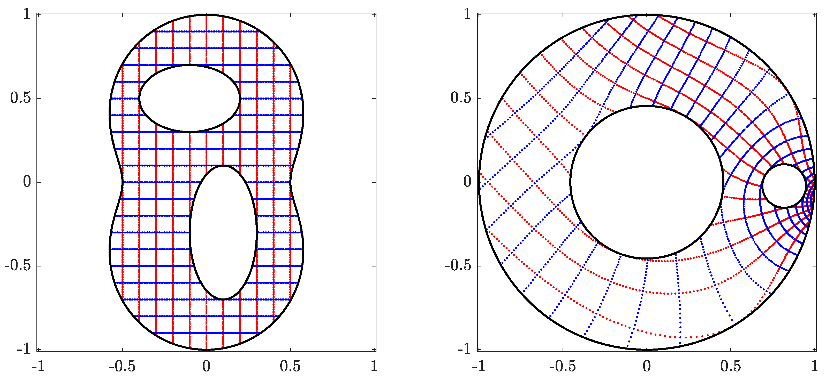
5.3. The Interior Points

Once the approximate boundary values of the mapping function w = ω ( z ) are obtained through (18), the values of w = ω ( z ) at interior points z G can be computed using the Cauchy integral formula,
w = ω ( z ) = 1 2 π i J ω ( ζ ( t ) ) ζ ( t ) z ζ ( t ) d t .
Since the derivative of ξ ( t ) = ω ( ζ ( t ) ) with respect to the parameter t is known, i.e., ξ ( t ) = ω ( ζ ( t ) ) ζ ( t ) , we can use the Cauchy integral formula to find the values of ω ( z ) for interior points z G , where
ω ( z ) = 1 2 π i J ω ( ζ ( t ) ) ζ ( t ) z ζ ( t ) d t = 1 2 π i J ξ ( t ) ζ ( t ) z d t .

5.4. The Inverse Circular Map

Since the boundary C of the domain Ω is parametrized by ξ ( t ) given by (18), the values of z = ω 1 ( w ) can be computed at interior points w Ω using the Cauchy integral formula
z = ω 1 ( w ) = 1 2 π i C ω 1 ( ξ ) ξ w d ξ = 1 2 π i J ω 1 ( ξ ( t ) ) ξ ( t ) w ξ ( t ) d t ,
where ω 1 ( ξ ( t ) ) = ζ ( t ) .

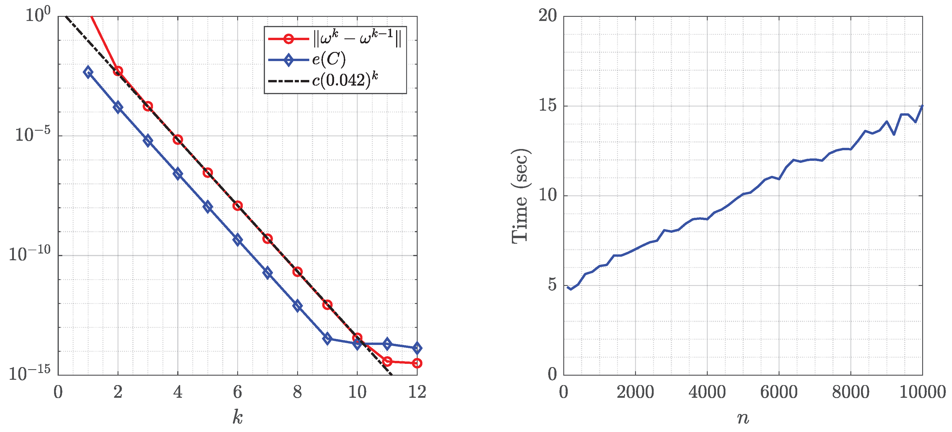
5.5. Computational Complexity

In each iteration of the generalized Koebe’s iterative method, the boundary values of approximately m / 2 conformal mappings of doubly connected domains are computed, which requires O ( m n log n ) operations. For each of these mappings, the Cauchy integral formula must be applied approximately m / 2 times, resulting in an additional computational cost of O ( m 2 n ) operations. Therefore, the total computational cost per iteration of the generalized Koebe’s method is O m n ( m + log n ) operations.

6. Numerical Examples

We consider five numerical examples. The domains for Examples 1 and 4 have been considered in [18] for computing the conformal mapping onto the circular domain using the classical Koebe’s method. The domain of Example 2 is a modification of the domain used in [29] for computing the conformal mapping onto circular and parallel slits domains. The domain for Example 5 has been considered in [22] for computing the conformal mapping onto a circular ring with circular hole domain using the generalized Koebe’s method implemented with the discrete Yamabe flow method. For all numerical examples, we compute the values of the conformal mapping for orthogonal grids in the given domain G and the values of the inverse conformal mapping for orthogonal grids in the computed domain Ω . In addition to computing the successive error, we compute the measurement of roundness e ( C ) which is defined by [22]
e ( C ) = 1 m + 1 j = 0 m e ( C j ) ,
where
e ( C j ) = 1 R j 1 n i = 1 n | d j , i R j | 2 , d j , i = | ξ j ( t i ) z j | .
The roundness error e ( C j ) measures how close the curve C j is from being a circle, where e ( C j ) = 0 when C j is a circle with center z j and radius R j .
The commuted successive error ω k ( ζ ) ω k 1 ( ζ ) and the roundness error e ( C ) illustrate that the proposed method converges after only a few iterations when the boundary components are well separated. The number of iterations increases for domains with close-to-touching boundary components. For all numerical examples, we estimate the rate of convergence p of the generalized Koebe’s iterative method, i.e., a real number 0 < p < 1 such that for k = 1 , 2 , 3 , and for ζ Γ ,
ω k ( ζ ) ω ( ζ ) c p k
for some constant c > 0 , where ω k ( ζ ) are the approximate boundary values and ω ( ζ ) are the exact boundary values of the conformal mapping. Since the exact boundary values are unknown, we estimate the value of p from the computed successive error ω k ( ζ ) ω k 1 ( ζ ) , i.e., we find p such that
ω k ( ζ ) ω k 1 ( ζ ) c p k .
Example 1.
In the first example, we calculate the conformal map w = ω ( z ) that maps the triply connected domain G in the exterior of the two ellipses
Γ 1 : ζ 1 ( t ) = 0.1 + 0.5 i + 0.3 cos t 0.2 i sin t , Γ 2 : ζ 2 ( t ) = + 0.1 0.3 i + 0.2 cos t 0.4 i sin t ,
and in the interior of the inverted ellipse
Γ 0 : ζ 0 ( t ) = 1 ( 1 ρ 2 ) cos 2 t e i t , ρ = 0.5 ,
for 0 t 2 π , onto the domain Ω obtained by removing a disk from a circular ring, where α = 0.2 i .
Figure 4 and Figure 5 show the original domain G, the image of G, the circular domain Ω , and the inverse image of Ω . The successive error ω k ω k 1 and the roundness error e ( C ) vs. the number of iteration k for k = 1 , 2 , , 12 are shown in Figure 6 (left). The line c p k is shown in Figure 6 (left) where the estimated rate of convergence is p = 0.042 . The run time in seconds as a function of n required by the generalized Koebe’s method when the number of iterations is fixed to be 12 for each n is shown in Figure 6 (right) which demonstrates that the CPU time depends almost linearly on n.
This example has been considered in ([18], Example 2) and ([23], Example 19) for computing the conformal mapping from G onto a circular domain using Koebe’s iterative method and Wegmann’s method, respectively. Note that the estimated rate of convergence for Koebe’s method in [18] is p = 0.049 .
Example 2.
In the second example, we calculate the conformal map w = ω ( z ) that maps the multiply connected domain G of connectivity 4 in the exterior of the curves
Γ 1 : ζ 1 ( t ) = 1 3 i + ( 1.2 + 0.4 cos ( 8 t ) ) e i t , Γ 2 : ζ 2 ( t ) = 2 + 2 i + ( 1.0 + 0.4 cos ( 6 t ) ) e i t , Γ 3 : ζ 3 ( t ) = 1 + ( 1.0 + 0.6 cos ( 4 t ) ) e i t ,
and in the interior of the curve
Γ 0 : ζ 0 ( t ) = ( 6 + 0.8 cos ( 18 t ) ) e i t ,
for 0 t 2 π , onto the domain Ω obtained by removing two disks from a circular ring, where α = 3.5 . The obtained numerical results are presented in Figure 7, Figure 8 and Figure 9.
Example 3.
In the third example, we calculate the conformal map w = ω ( z ) that maps the triply connected domain G in the exterior of the ellipses
Γ 1 : ζ 1 ( t ) = 0.7 i + 0.08 cos t 0.8 i sin t , Γ 2 : ζ 2 ( t ) = 0.9 + cos t 0.7 i sin t ,
and in the interior of the ellipse
Γ 0 : ζ 0 ( t ) = 2 cos t + i sin t ,
for 0 t 2 π , onto the domain Ω obtained by removing a disk from a circular ring, where α = 0.3 . The obtained numerical results are presented in Figure 10, Figure 11 and Figure 12. The boundary components of the domain G are close to each other so that, as expected, the method requires more iterations to converge compared to the previous two examples.
Example 4.
In the fourth example, we consider a multiply connected domain with high connectivity as shown in Figure 13. We calculate the conformal map w = ω ( z ) that maps a multiply connected domain G with connectivity 100 onto the domain Ω obtained by removing 98 disks from a circular ring. The obtained numerical results are presented in Figure 13, Figure 14 and Figure 15.
Example 5.
We consider a face domain G with four boundary components from ([22], Figure 8). The boundary points are extracted from the image and the parametrizations of the boundary components are approximated using piecewise periodic cubic spline interpolation.
Figure 16 and Figure 17 show the original domain G, the image of G, the circular domain Ω , and the inverse image of Ω . The original image and the mapped image in a circular ring with circular holes are show in Figure 18. The successive error ω k ω k 1 and the roundness error e ( C ) vs. the number of iteration k for k = 1 , 2 , , 20 are shown in Figure 19. The line c p k is also shown in Figure 19, where the estimated rate of convergence is p = 0.045 . The successive and the roundness errors presented in Figure 19 illustrated that the proposed method converges with sufficient accuracy after only 7 iterations.
For this example, we have m = 3 and hence each iteration of our implementation of the generalized Koebe’s method requires two steps (two computations of conformal mappings from unbounded doubly connected domains onto a circular ring). The roundness error for the first two steps (first iteration) of the proposed method is presented in Table 1. This table also presents the roundness error for the first five steps of the method presented in [22] (see [22], Figure 4 and Table 2). It is clear from Table 1 that the roundness error for the proposed method after only two steps is much less than the roundness error for the method presented in [22] after five steps.

7. Conclusions

This paper presented a new, fast and efficient numerical implementation of generalized Koebe’s method for computing the conformal mapping from bounded multiply connected domains onto circular ring with circular holes domains. The method is based on using the boundary integral equation with the generalized Neumann kernel. Five numerical examples were presented to illustrate the accuracy and efficiency of the proposed method. The number of iterations of the generalized Koebe’s method and the CPU time (in seconds) required for the convergence for the five examples is presented in Table 2. Compared to the method presented in [22], the proposed method demonstrates a higher convergence rate and enables the computation of the conformal mapping, its derivative, and its inverse. We consider only domains with smooth boundaries in this paper. However, the proposed method can be extended to domains with piecewise smooth boundaries using the same approach used in [18,19,25].

Author Contributions

Conceptualization, K.W.L., A.H.M.M., M.M.S.N. and S.H.Y.; Methodology, K.W.L., A.H.M.M. and S.H.Y.; Software, K.W.L. and M.M.S.N.; Validation, K.W.L., A.H.M.M. and S.H.Y.; Writing—original draft, K.W.L., A.H.M.M. and M.M.S.N.; Writing—review & editing, K.W.L., A.H.M.M., M.M.S.N. and S.H.Y. All authors have read and agreed to the published version of the manuscript.

Funding

The first author would like to acknowledge the partial financial support for his research study from the Ministry of Higher Education Malaysia under Fundamental Research Grant Scheme (FRGS/1/2019/STG06/UTM/02/20) and from Universiti Teknologi Malaysia under UTM Fundamental Research (UTMFR) (QJ130000.2554.20H72).

Data Availability Statement

The MATLAB codes used to generate the figures and tables in this paper are available at https://github.com/mmsnasser/gkmethod (accessed on 1 June 2025).

Acknowledgments

The authors would like to thank the anonymous reviewers for their valuable comments and suggestions which improved the presentation of this paper.

Conflicts of Interest

The authors declare no conflicts of interest.

References

  1. Crowdy, D.G. Solving Problems in Multiply Connected Domains; SIAM: Philadelphia, PA, USA, 2020. [Google Scholar]
  2. Schiffer, M. Recent advances in the theory of conformal mapping, appendix to: R. Courant. In Dirichlet’s Principle, Conformal Mapping, and Minimal Surfaces; Interscience Publishers: New York, NY, USA, 1950. [Google Scholar]
  3. Henrici, P. Applied and Computational Complex Analysis; John Wiley: New York, NY, USA, 1986; Volume 3. [Google Scholar]
  4. Koebe, P. Abhandlungen zur Theorie der konformen Abbildung, IV. Abbildung mehrfach zusammenhängender schlichter Bereiche auf Schlitzbe-reiche. Acta Math. 1918, 41, 305–344. [Google Scholar] [CrossRef]
  5. Wen, G.C. Conformal Mapping and Boundary Value Problems; American Mathematical Society: Providence, RI, USA, 1992. [Google Scholar]
  6. Crowdy, D. Conformal slit maps in applied mathematics. ANZIAM J. 2012, 53, 171–189. [Google Scholar]
  7. Nasser, M.M.S. Numerical conformal mapping via a boundary integral equation with the generalized Neumann kernel. SIAM J. Sci. Comput. 2009, 31, 1695–1715. [Google Scholar] [CrossRef]
  8. Nasser, M.M.S. Numerical conformal mapping of multiply connected regions onto the second, third and fourth categories of Koebe’s canonical slit domains. J. Math. Anal. Appl. 2009, 382, 47–56. [Google Scholar] [CrossRef]
  9. Nasser, M.M.S. Numerical conformal mapping of multiply connected regions onto the fifth category of Koebe’s canonical slit regions. J. Math. Anal. Appl. 2013, 398, 729–743. [Google Scholar] [CrossRef]
  10. Nasser, M.M.S.; Al-Shihri, F.A.A. A Fast Boundary Integral Equation Method for Conformal Mapping of Multiply Connected Regions. SIAM J. Sci. Comput. 2013, 35, A1736–A1760. [Google Scholar] [CrossRef]
  11. Koebe, P. Über die Uniformisierung der algebraischen Kurven. II. Math. Ann. 1910, 69, 1–81. [Google Scholar] [CrossRef]
  12. Marshall, D. Conformal welding for finitely connected regions. Comput. Methods Funct. Theory 2011, 11, 655–669. [Google Scholar] [CrossRef]
  13. Benchama, N.; DeLillo, T.; Hrycak, T.; Wang, L. A simplified Fornberg-like method for the conformal mapping of multiply connected regions–Comparisons and crowding. J. Comput. Appl. Math. 2007, 209, 1–21. [Google Scholar] [CrossRef]
  14. DeLillo, T.K.; Elcrat, A.R.; Pfaltzgraff, J.A. Schwarz–Christoffel mapping of multiply connected domains. J. Anal. Math. 2004, 94, 17–47. [Google Scholar] [CrossRef]
  15. Kropf, E.; Yin, X.; Yau, S.; Gu, X. Conformal parameterization for multiply connected domains: Combining finite elements and complex analysis. Eng. Comput. 2014, 30, 441–455. [Google Scholar] [CrossRef]
  16. Gu, X.; Zeng, W.; Luo, F.; Yau, S. Numerical computation of surface conformal mappings. Comput. Methods Funct. Theory 2011, 11, 747–787. [Google Scholar] [CrossRef]
  17. Luo, W.; Dai, J.; Gu, X.; Yau, S. Numerical conformal mapping of multiply connected domains to regions with circular boundaries. J. Comput. Appl. Math. 2010, 233, 2940–2947. [Google Scholar] [CrossRef]
  18. Nasser, M.M.S. Fast computation of the circular map. Comput. Methods Funct. Theory 2015, 15, 187–223. [Google Scholar] [CrossRef]
  19. Nasser, M.M.S. PlgCirMap: A MATLAB toolbox for computing conformal mappings from polygonal multiply connected domains onto circular domains. SoftwareX 2020, 11, 100464. [Google Scholar] [CrossRef]
  20. Zhang, M.; Li, Y.; Zeng, W.; Gu, X. Canonical conformal mapping for high genus surfaces with boundaries. Comput. Graph. 2012, 36, 417–426. [Google Scholar] [CrossRef]
  21. Wegmann, R. Fast conformal mapping of multiply connected regions. J. Comput. Appl. Math. 2001, 130, 119–138. [Google Scholar] [CrossRef]
  22. Zeng, W.; Yin, X.; Zhang, M.; Luo, F.; Gu, X. Generalized Koebe’s method for conformal mapping multiply connected domains. In Proceedings of the SIAM/ACM Joint Conference on Geometric and Physical Modeling, San Francisco, CA, USA, 5–8 October 2009; pp. 89–100. [Google Scholar]
  23. Wegmann, R. Methods for numerical conformal mapping. In Handbook of Complex Analysis: Geometric Function Theory; Kühnau, R., Ed.; Elsevier B. V.: Amsterdam, The Netherlands, 2005; Volume 2, pp. 351–477. [Google Scholar]
  24. Wegmann, R.; Nasser, M.M.S. The Riemann-Hilbert problem and the generalized Neumann kernel on multiply connected regions. J. Comput. Appl. Math. 2008, 214, 36–57. [Google Scholar] [CrossRef]
  25. Nasser, M.M.S. Fast solution of boundary integral equations with the generalized Neumann kernel. Electron. Trans. Numer. Anal. 2015, 44, 189–229. [Google Scholar]
  26. Nasser, M.M.S.; Murid, A.H.M.; Ismail, M.; Alejaily, E.M.A. Boundary integral equations with the generalized Neumann kernel for Laplace’s equation in multiply connected regions. Appl. Math. Comput. 2011, 217, 4710–4727. [Google Scholar] [CrossRef]
  27. Atkinson, K.E. The Numerical Solution of Integral Equations of the Second Kind; Cambridge University Press: Cambridge, UK, 1997. [Google Scholar]
  28. Greengard, L.; Gimbutas, Z. FMMLIB2D: A MATLAB Toolbox for Fast Multipole Method in Two Dimensions, Version 1.2. 2019. Available online: https://github.com/zgimbutas/fmmlib2d (accessed on 1 February 2024).
  29. Sangawi, A.W.K.; Murid, A.H.M.; Lee, K.W. Conformal mappings of bounded multiply connected regions onto circular and parallel slits regions and their inverses using a GUI. ScienceAsia 2017, 43S, 79–89. [Google Scholar] [CrossRef]
Figure 1. A schematic of a given bounded multiply connected domain G of connectivity m + 1 (left) and its conformally equivalent computed domain Ω obtained by removing m 1 disks from a circular ring (right).
Mathematics 13 01920 g001
Figure 2. A schematic of a given bounded multiply connected domain G of connectivity six ( m = 5 ) and the three intermediate domains computed in the first iteration of generalized Koebe’s method, which involves three steps where each step requires computing the conformal mapping from an unbounded doubly connected domain onto a circular ring.
Mathematics 13 01920 g002
Figure 3. A schematic of a given bounded multiply connected domain G of connectivity six ( m = 5 ) and its conformally equivalent image domain Ω computed in the first five iterations of generalized Koebe’s method.
Mathematics 13 01920 g003
Figure 4. The original domain G for Example 1 (left) and its image obtained with n = 1024 (right).
Mathematics 13 01920 g004
Figure 5. The circular domain Ω for Example 1 (left) and its inverse image obtained with n = 1024 (right).
Mathematics 13 01920 g005
Figure 6. Left: The successive error and the roundness error e ( C ) for Example 1 obtained with n = 1024 . Right: Run time in seconds as a function of n required by the generalized Koebe’s method after 12 iterations for each n.
Mathematics 13 01920 g006
Figure 7. The original domain G for Example 2 (left) and its image obtained with n = 1024 (right).
Mathematics 13 01920 g007
Figure 8. The circular domain Ω for Example 2 (left) and its inverse image obtained with n = 1024 (right).
Mathematics 13 01920 g008
Figure 9. The successive error and the roundness error e ( C ) for Example 2 obtained with n = 1024 .
Mathematics 13 01920 g009
Figure 10. The original domain G for Example 3 (left) and its image obtained with n = 1024 (right).
Mathematics 13 01920 g010
Figure 11. The circular domain Ω for Example 3 (left) and its inverse image obtained with n = 1024 (right).
Mathematics 13 01920 g011
Figure 12. The successive error the roundness error e ( C ) for Example 3 obtained with n = 1024 .
Mathematics 13 01920 g012
Figure 13. The original domain G for Example 4 (left) and its image obtained with n = 1024 (right).
Mathematics 13 01920 g013
Figure 14. The circular domain Ω for Example 4 (left) and its inverse image obtained with n = 1024 (right).
Mathematics 13 01920 g014
Figure 15. The successive error the roundness error e ( C ) for Example 4 obtained with n = 1024 .
Mathematics 13 01920 g015
Figure 16. The original domain G for Example 5 (left) and its image obtained with n = 4096 (right).
Mathematics 13 01920 g016
Figure 17. The circular domain Ω for Example 5 (left) and its inverse image obtained with n = 4096 (right).
Mathematics 13 01920 g017
Figure 18. Image transformation of a human face domain onto a circular ring with two circular holes.
Mathematics 13 01920 g018
Figure 19. The successive error the roundness error e ( C ) for Example 5 obtained with n = 4096 .
Mathematics 13 01920 g019
Table 1. A comparison between our implementation of the generalized Koebe’s method and the implementation presented in [22].
MethodStepsTime (sec)Roundness Error e(C)
Zeng et al. [22]  54860.143825
Our method21.620.009606
Table 2. The number of iterations and the CPU time (in seconds) required for the convergence of the generalized Koebe’s method for Examples 1–5.
ExamplemnIterationsTime (s)
121024126.20
231024107.45
3210245025.84
4991024121259.67
5340961513.43
Disclaimer/Publisher’s Note: The statements, opinions and data contained in all publications are solely those of the individual author(s) and contributor(s) and not of MDPI and/or the editor(s). MDPI and/or the editor(s) disclaim responsibility for any injury to people or property resulting from any ideas, methods, instructions or products referred to in the content.

