


Optimal Design of Variable-Stiffness Fiber-Reinforced Composites


Abstract
1. Introduction
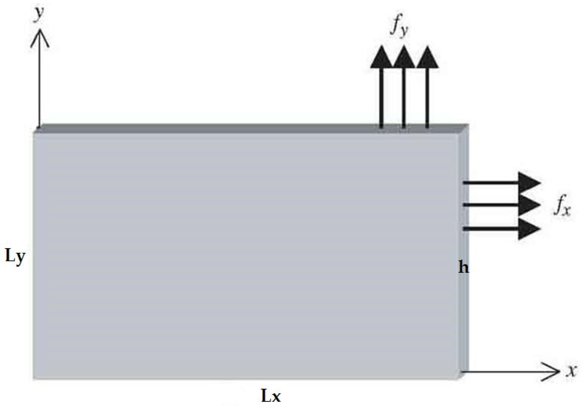
2. The Mathematical Model
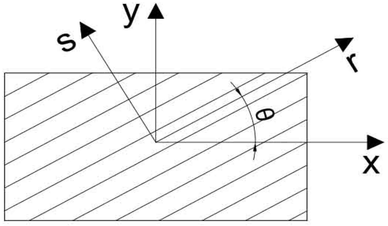
2.1. Kinematics and Constitutive Relationships
2.2. Governing Equations and Boundary Conditions
2.2.1. Equations of Motion and Boundary Conditions in Expanded Form
- Equations of motion:
- Boundary conditions:
2.2.2. Equations of Motion and Boundary Conditions in Vector Form
- Equations of motion:
- Boundary conditions:
2.2.3. The Stiffness Matrix of a Fiber-Reinforced Composite Layer
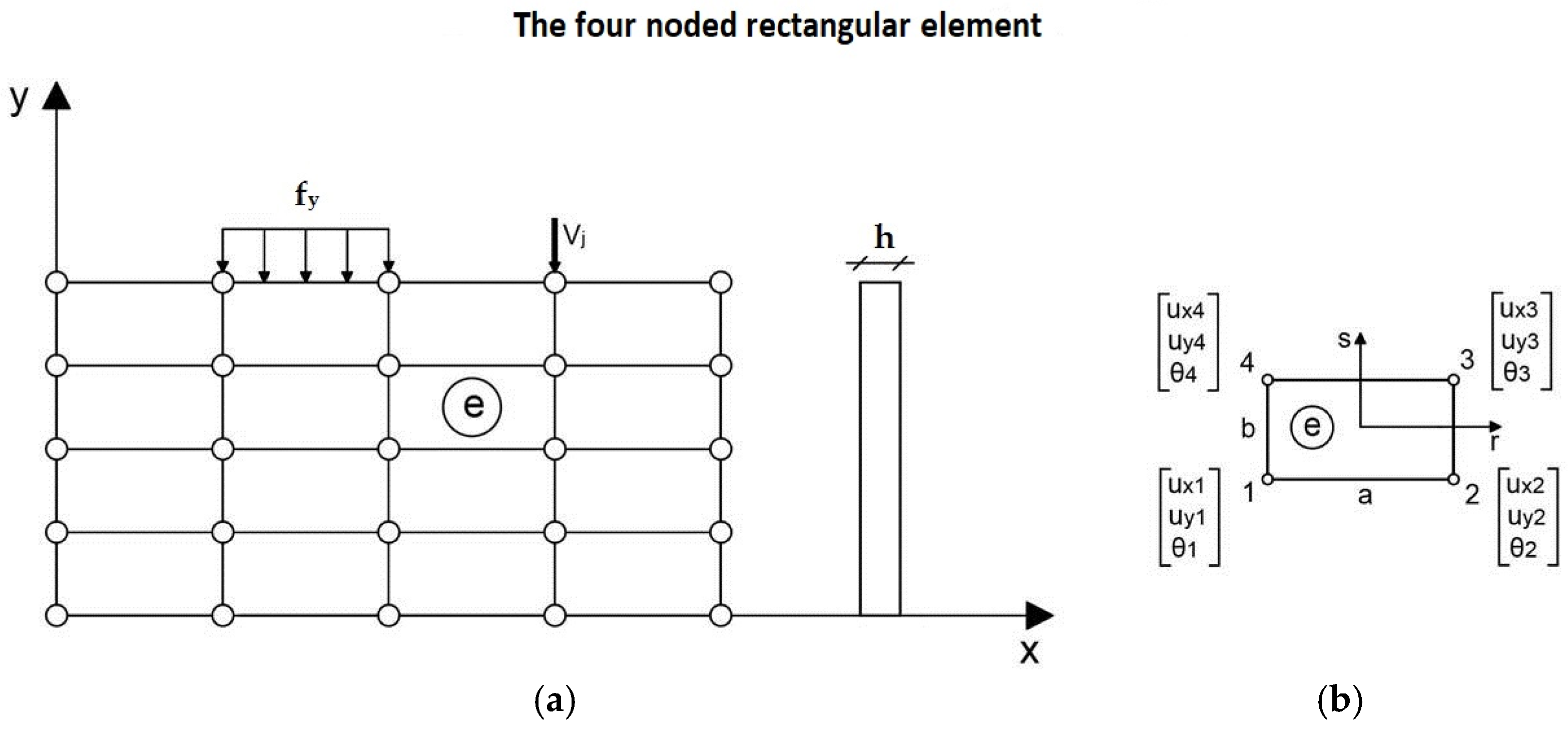
3. Finite Element Formulation
4. The Optimization Problem
4.1. The Optimal Design Problem
- Optimal Design Problem (ODP). For an elastic fiber-reinforced composite plate subject to equilibrium constraint, find the value of the design vector variable (values of fiber angle in each element), so that the strain energy of the structure to be minimized.
4.2. The Genetic Algorithm Optimization Method
- Selection rules select the individuals, called parents, who contribute to the population in the next generation.
- Crossover rules combine two parents to create children for the next generation.
- Mutation rules apply random changes to each parent to create children.
- The following outline summarizes how the genetic algorithm works:
- The algorithm starts by generating a random initial population.
- The algorithm then generates a sequence of new populations. At each step, the algorithm uses the individuals in the current generation to create the next population. To create the new population, the algorithm
- Assesses each member of the current population by calculating their fitness value. These values are called the raw fitness scores;
- Scales the raw fitness scores to convert them into a more usable range of values. These scaled values are referred to as expectation values;
- Selects members, called parents, based on their expectations;
- Selects some of the individuals in the current population that have lower fitness, called elite. These elite individuals are passed on to the next population;
- Generates children from parents. Children are produced either by making random changes to a single parent—i.e., a mutation—or by combining the vector entries of a pair of parents—i.e., a crossover;
- Replaces the current population with children to form the next generation.
- The algorithm stops when one of the stopping criteria is met.
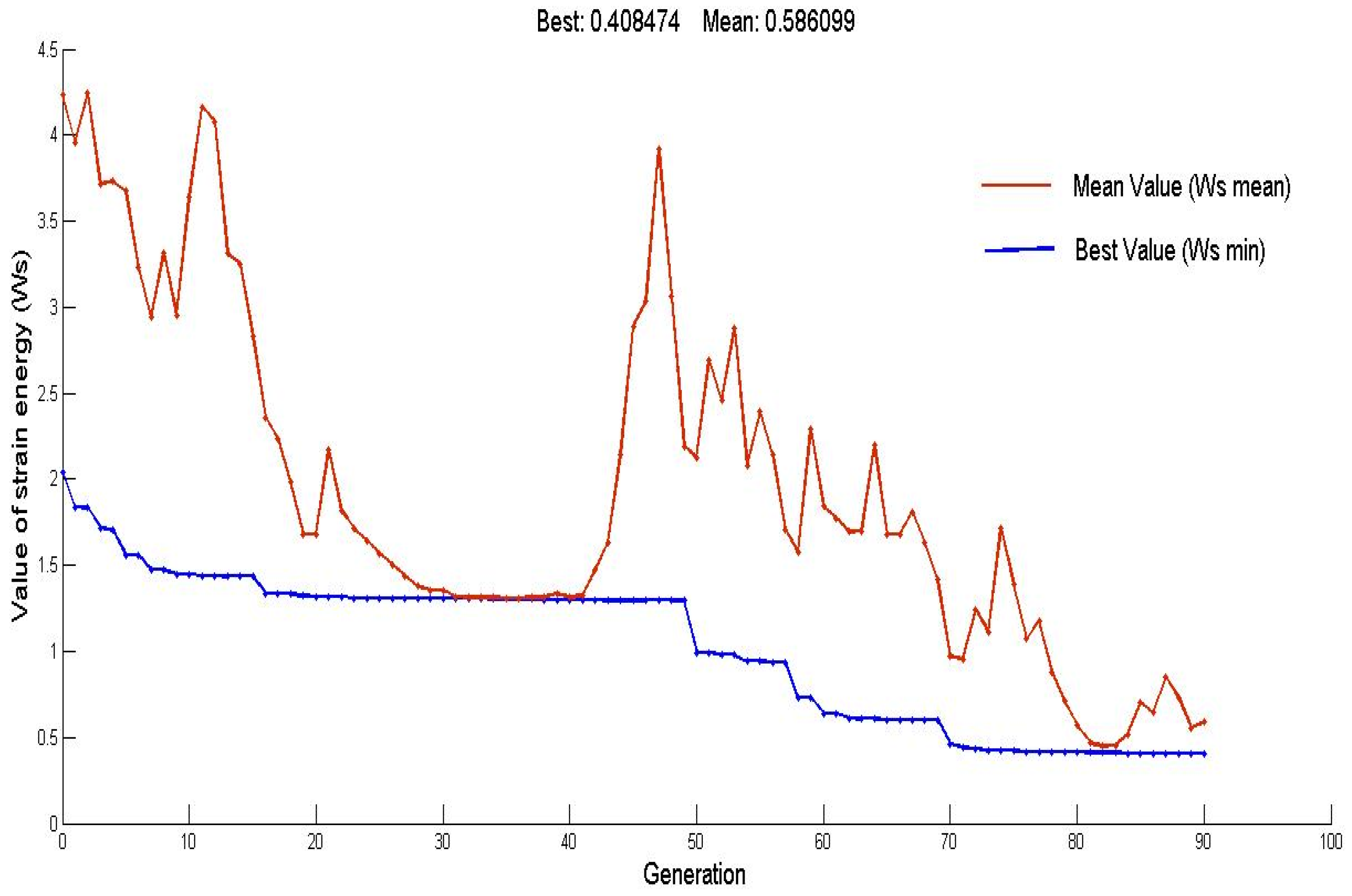
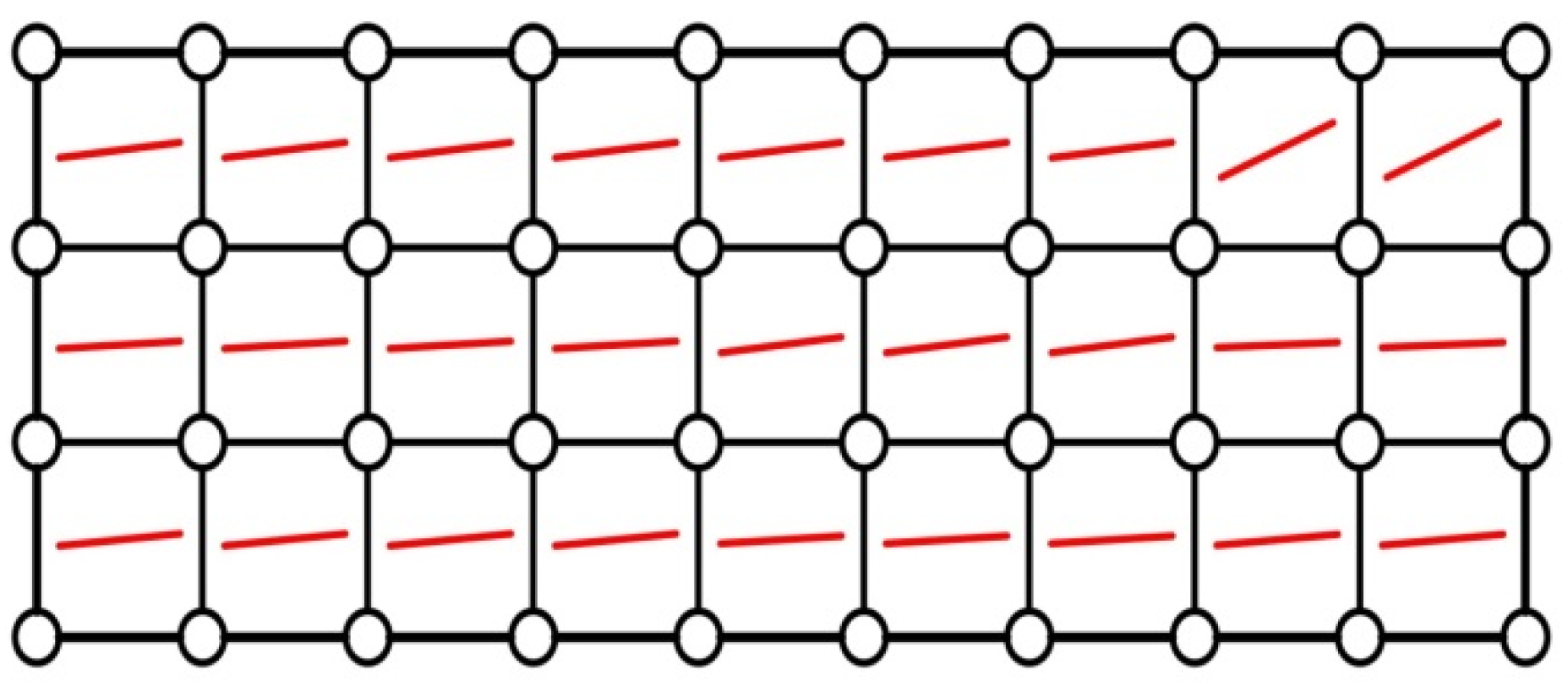
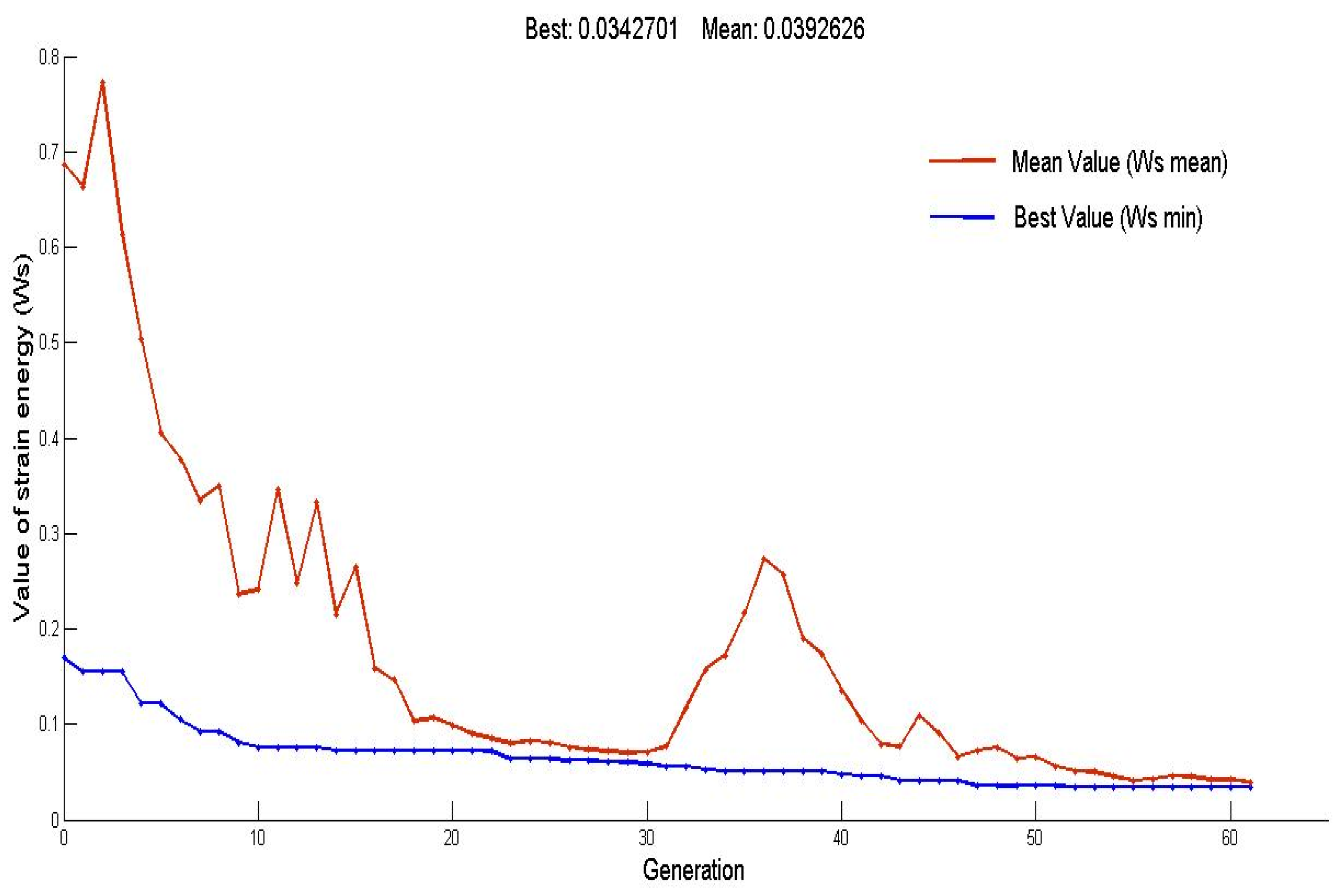
5. Numerical Examples and Discussion
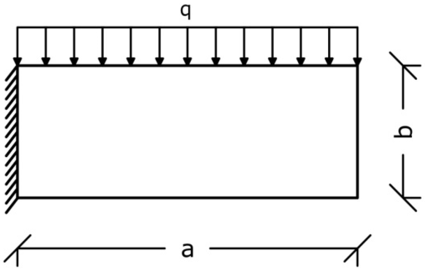
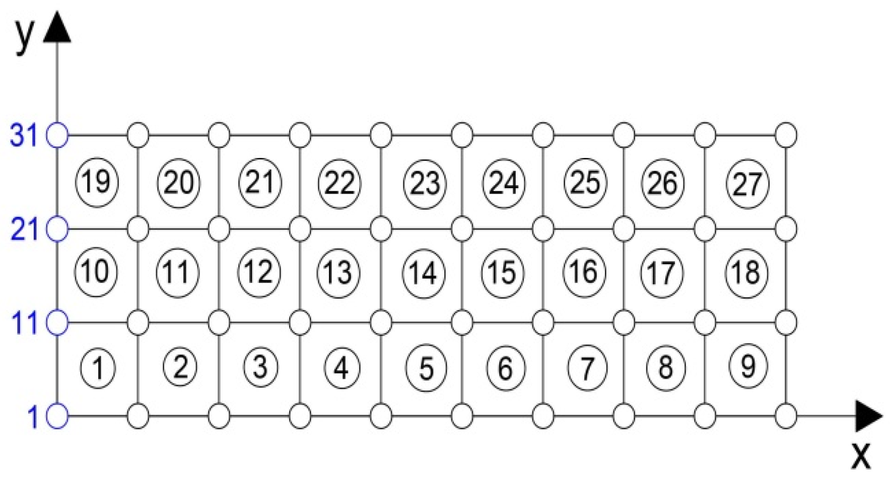
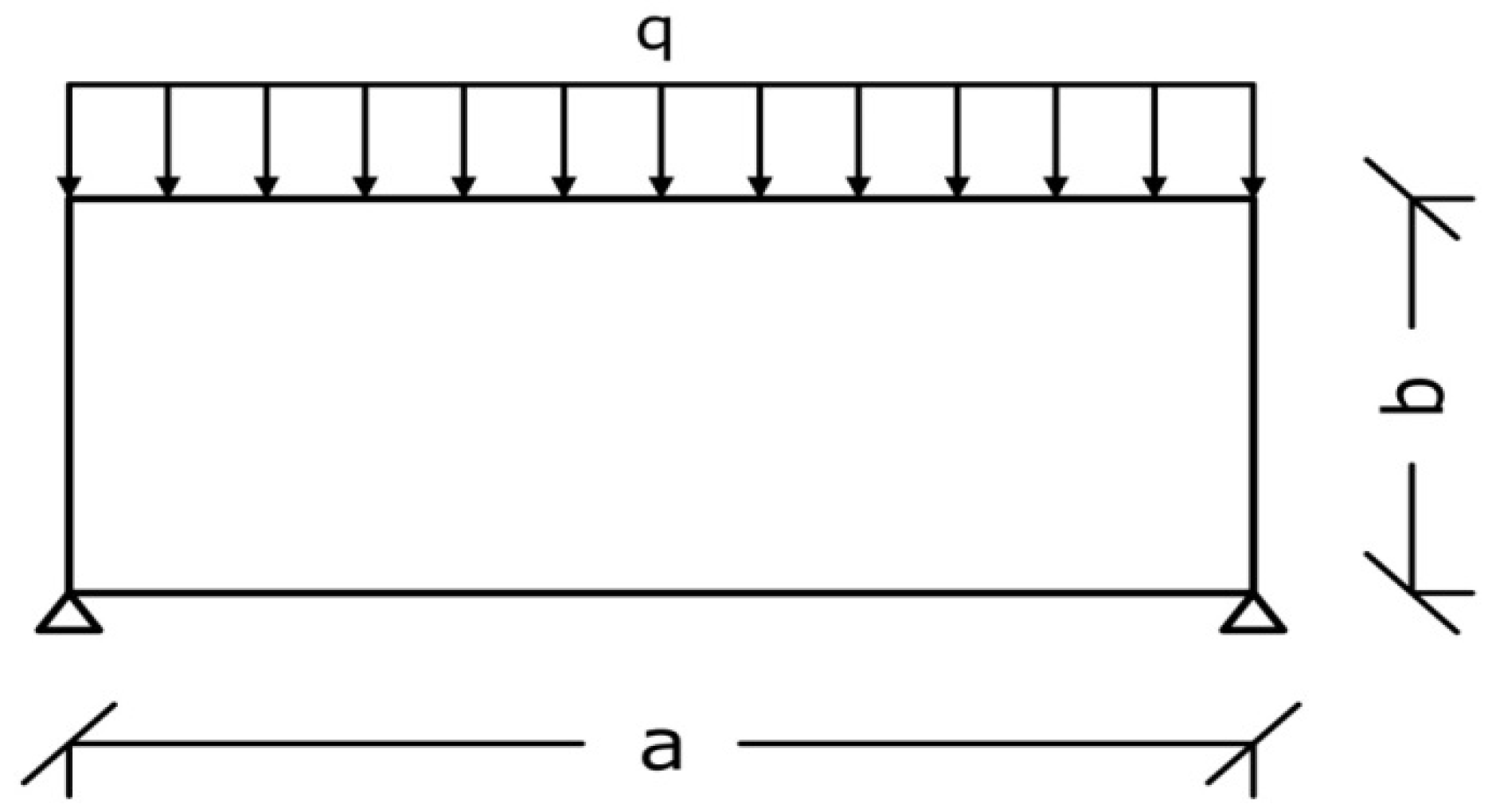
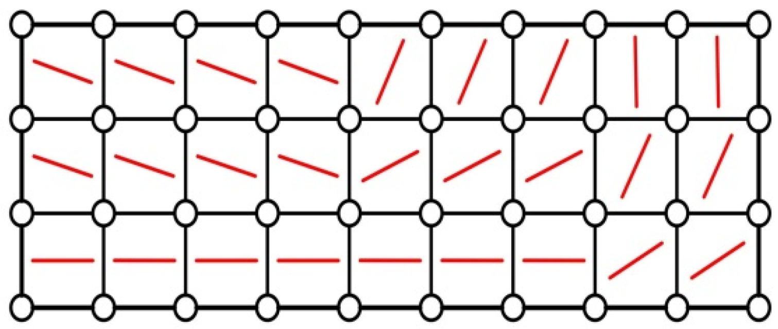
5.1. Example 1
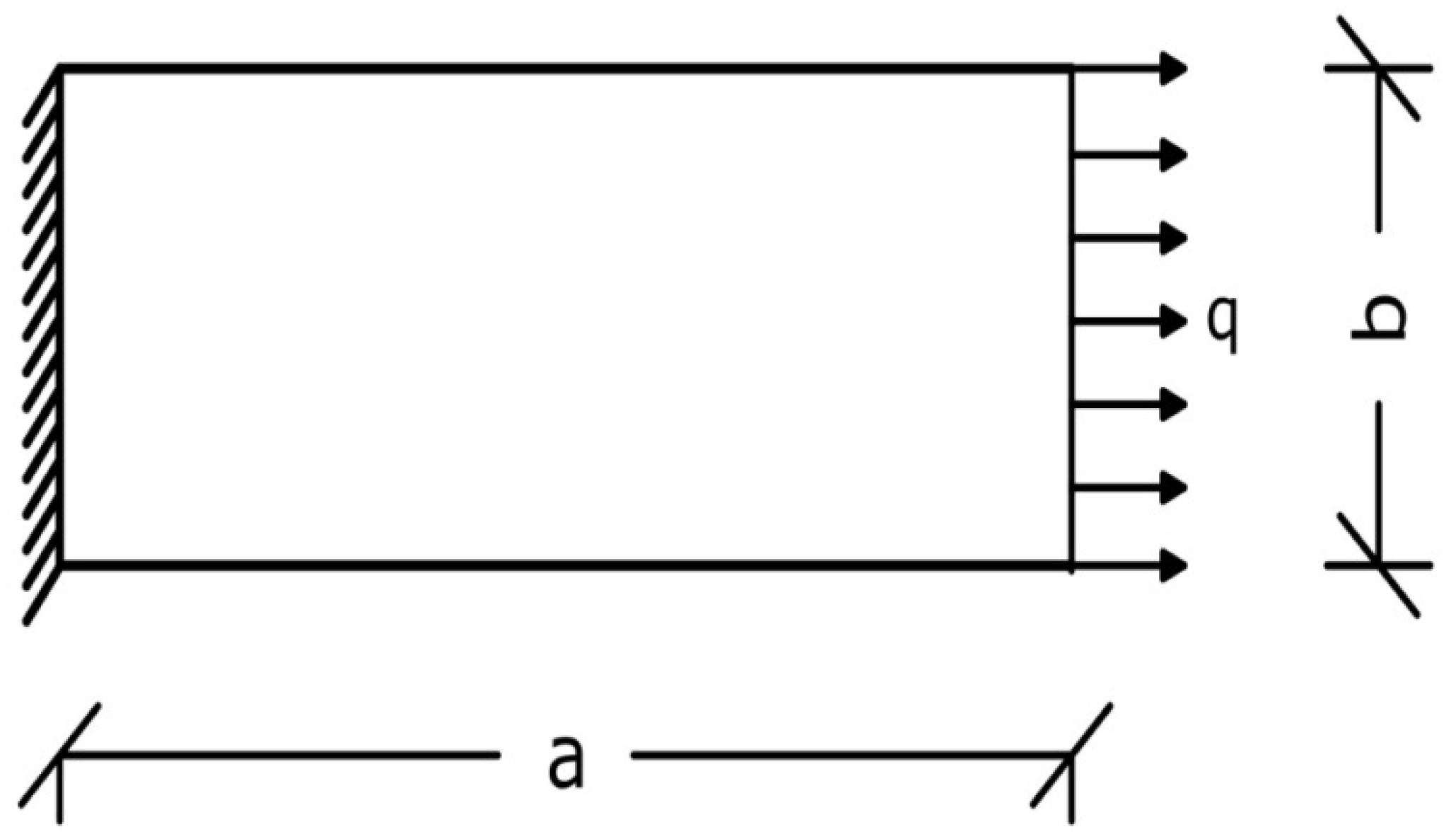
5.2. Example 2
5.3. Example 3
6. Conclusions
- In order to make the composite material as stiff as possible, an optimal design problem (ODP) for the curvilinear reinforcing fibers has been defined and solved numerically.
- The optimization problem is highly non-linear and non-convex due to the presence of trigonometric functions. For these reasons, a global optimization method based on genetic algorithms is used.
- Based on the strain energy-minimizing method, a finite element formulation is used to solve the equilibrium equations of the structure each time, and a genetic algorithm method is used to solve the strain energy minimization problem.
- Three numerical examples are presented in support of the proposed theoretical and numerical scheme.
- In all examples, fast convergence of the proposed scheme was observed. The mean and minimum values of strain energy in each generation converged after about 50 generations in the first example, 80 generations in the second example, and about 60 generations in the third example, with a maximum number of generations equal to 100.
- While many aspects of the proposed methodology require further study, the numerical examples in Section 5 show that the solutions obtained consistently align with the theoretical predictions of the principal stress trajectories within the structure. As is well known, reinforcement in composites is generally positioned along or across these tensile trajectories. The results obtained thus far validate the proposed methodological approach.
- The proposed method can also be used to study reinforcement fibers of various shapes, including squares and ellipses. In such cases, it would be interesting to study the final shape of the curved fibers and their relationship with geometric characteristics.
- The proposed method can also be improved by using more accurate elements to achieve better convergence and more precise results.
- This study presents a straightforward method to optimize the shape of curvilinear fibers in fiber-reinforced composite materials. The proposed method is based on the appropriate arrangement of fiber angles, which change continuously and independently at design points—for example, at the centers of finite elements in the present work. The flexibility of independently optimizing fiber angles at different design points creates difficulties that must be carefully studied in the near future. For example, the resulting optimal design often has a discontinuous fiber path, leading in a structure that cannot be manufactured and the concentration of stress. Additionally, the non-convexity of the optimization problem and the large number of design variables make the solution sensitive to the initial design and potentially sub-optimal.
Author Contributions
Funding
Data Availability Statement
Conflicts of Interest
References
- Kartsonakis, I. Progress of Fiber-Reinforced Composites Design and Applications; MDPI Books: Basel, Switzerland, 2022. [Google Scholar] [CrossRef]
- Rajak, D.K.; Pagar, D.D.; Menezes, P.L.; Linul, E. Fiber-Reinforced Polymer Composites: Manufacturing, Properties, and Applications. Polymers 2019, 11, 1667. [Google Scholar] [CrossRef] [PubMed]
- Mallick, P.K. Fiber-Reinforced Composites: Materials, Manufacturing, and Design, 3rd ed.; CRC Press: Boca Raton, FL, USA, 2007. [Google Scholar] [CrossRef]
- Campbell, F.C. Structural Composite Materials; ASM International: Novelty, OH, USA, 2010. [Google Scholar] [CrossRef]
- Agarwal, B.D.; Broutman, L.J.; Chandrashekhara, K. Analysis and Performance of Fiber Composites, 4th ed.; John Wiley & Sons: Hoboken, NJ, USA, 2018; ISBN 978-1-119-38998-9. [Google Scholar]
- Ashrith, H.S.; Jeevan, T.P.; Xu, J. A Review on the Fabrication and Mechanical Characterization of Fibrous Composites for Engineering Applications. J. Compos. Sci. 2023, 7, 252. [Google Scholar] [CrossRef]
- Liampas, S.; Kladovasilakis, N.; Tsongas, K.; Pechlivani, E.M. Recent Advances in Additive Manufacturing of Fibre-Reinforced Materials: A Comprehensive Review. Appl. Sci. 2024, 14, 10100. [Google Scholar] [CrossRef]
- Xin, Z.; Duan, Y.; Xu, W.; Zhang, T.; Wang, B. Review of the mechanical performance of variable stiffness design fiber-reinforced composites. Sci. Eng. Compos. Mater. 2016, 25, 425–437. [Google Scholar] [CrossRef]
- Marques, F.E.C.; Mota, A.F.S.d.; Loja, M.A.R. Variable Stiffness Composites: Optimal Design Studies. J. Compos. Sci. 2020, 4, 80. [Google Scholar] [CrossRef]
- Arranz, S.; Sohouli, A.; Suleman, A. Buckling Optimization of Variable Stiffness Composite Panels for Curvilinear Fibers and Grid Stiffeners. J. Compos. Sci. 2021, 5, 324. [Google Scholar] [CrossRef]
- Gürdal, Z.; Haftka, R.; Hajela, P. Design and Optimization of Laminated Composite Materials; Wiley: New York, NY, USA, 1999. [Google Scholar]
- Gürdal, Z.; Olmedo, R. In-plane response of laminates with spatially varying fibre orientations: Variable stiffness concept. AIAA J. 1993, 31, 751–758. [Google Scholar] [CrossRef]
- Pedersen, P. Examples of density, orientation, and shape-optimal 2d-design for stiffness and/or strength with orthotropic materials. Struct. Multidisc. Optim. 2004, 26, 37–49. [Google Scholar] [CrossRef]
- Setoodeh, S.; Abdalla, M.M.; Gürdal, Z. Design of variable-stiffness laminates using lamination parameters. Compos. Part B 2005, 37, 301–309. [Google Scholar] [CrossRef]
- Setoodeh, S.; Gürdal, Z.; Watson, L.T. Design of variable-stiffness composite layers using cellular automata. Comput. Methods Appl. Mech. Eng. 2006, 195, 836–851. [Google Scholar] [CrossRef]
- Wiśniewski, J. Optimal Design of Reinforcing Fibres in Multilayer Composites using Genetic Algorithms. Fibres Text. East. Eur. 2004, 12, 58–63. [Google Scholar]
- Berthelot, J.-M. Composite Materials; Springer: New York, NY, USA, 1999. [Google Scholar] [CrossRef]
- Zienkiewicz, O.C.; Taylor, R.L.; Zhu, J.Z. The Finite Element Method: Its Basis and Fundamentals, 7th ed.; Elsevier Ltd.: Oxford, UK, 2013. [Google Scholar]
- Kwon, Y.W.; Bang, H. The Finite Element Method Using MATLAB; CRC Press: Boca Raton, FL, USA, 2000. [Google Scholar]
- Kramer, O. Genetic Algorithm Essentials; Springer: Cham, Switzerland, 2017. [Google Scholar] [CrossRef]
- Khayyam, H.; Jamali, A.; Assimi, H.; Jazar, R.N. Genetic Programming Approaches in Design and Optimization of Mechanical Engineering Applications. In Nonlinear Approaches in Engineering Applications; Jazar, R., Dai, L., Eds.; Springer: Cham, Switzerland, 2020; pp. 367–402. [Google Scholar] [CrossRef]
- Hwang, S.F.; Hsu, Y.C.; Chen, Y. A genetic algorithm for the optimization of fiber angles in composite laminates. J. Mech. Sci. Technol. 2014, 28, 3163–3169. [Google Scholar] [CrossRef]
- Hadjigeorgiou, E.P.; Stavroulakis, G.E.; Massalas, C.V. Shape control and damage identification of beams using piezoelectric actuation and genetic optimization. Int. J. Eng. Sci. 2006, 44, 409–421. [Google Scholar] [CrossRef]
- Corriveau, G.; Guilbault, R.; Tahan, A. Genetic algorithms and finite element coupling for mechanical optimization. Adv. Eng. Softw. 2010, 41, 422–426. [Google Scholar] [CrossRef]


| Elements | 1–4 | 5–7 | 8–9 | 10–13 | 14–16 | 17–18 | 19–22 | 23–25 | 26–27 |
|---|---|---|---|---|---|---|---|---|---|
| Optimal value of θ (degrees) | 180 | 179.8385 | 30.1669 | 163.4943 | 24.7098 | 62.6838 | 161.9752 | 64.0427 | 91.3530 |
| Elements | 1–4 | 5 | 6–9 | 10–13 | 14 | 15–18 | 19–22 | 23 | 24–27 |
|---|---|---|---|---|---|---|---|---|---|
| Optimal value of θ (degrees) | 51.8807 | 36.5027 | 130.12024 | 43.5890 | 125.0221 | 136.2704 | 13.5154 | 1.7260 | 166.6832 |
| Elements | 1–4 | 5–7 | 8–9 | 10–13 | 14–16 | 17–18 | 19–22 | 23–25 | 26–27 |
|---|---|---|---|---|---|---|---|---|---|
| Optimal value of θ (degrees) | 4.7918 | 3.0911 | 4.3718 | 3.0246 | 6.1999 | 2.1623 | 6.0857 | 6.1747 | 22.4719 |
Disclaimer/Publisher’s Note: The statements, opinions and data contained in all publications are solely those of the individual author(s) and contributor(s) and not of MDPI and/or the editor(s). MDPI and/or the editor(s) disclaim responsibility for any injury to people or property resulting from any ideas, methods, instructions or products referred to in the content. |
© 2025 by the authors. Licensee MDPI, Basel, Switzerland. This article is an open access article distributed under the terms and conditions of the Creative Commons Attribution (CC BY) license (https://creativecommons.org/licenses/by/4.0/).
Share and Cite
Hadjigeorgiou, E.P.; Patsouras, C.A.; Kalpakides, V.K. Optimal Design of Variable-Stiffness Fiber-Reinforced Composites. Mathematics 2025, 13, 1909. https://doi.org/10.3390/math13121909
Hadjigeorgiou EP, Patsouras CA, Kalpakides VK. Optimal Design of Variable-Stiffness Fiber-Reinforced Composites. Mathematics. 2025; 13(12):1909. https://doi.org/10.3390/math13121909
Chicago/Turabian StyleHadjigeorgiou, Evangelos P., Christos A. Patsouras, and Vassilios K. Kalpakides. 2025. "Optimal Design of Variable-Stiffness Fiber-Reinforced Composites" Mathematics 13, no. 12: 1909. https://doi.org/10.3390/math13121909
APA StyleHadjigeorgiou, E. P., Patsouras, C. A., & Kalpakides, V. K. (2025). Optimal Design of Variable-Stiffness Fiber-Reinforced Composites. Mathematics, 13(12), 1909. https://doi.org/10.3390/math13121909