Asymptotic Behavior of the Modulus of the Kernel and Error Bounds of Anti-Gaussian Quadrature Formulas with Jacobi Weights

Abstract

In this paper, the remainder term of anti-Gaussian quadrature rules for analytic integrands with respect to Jacobi weight functions ${\omega }_{a,b}\left(x\right)={(1-x)}^a{(1+x)}^b$, where $a,b>-1$, is analyzed, and sharp estimates of the error are provided. These kinds of quadrature formulas were introduced by D.P. Laurie and have been recently studied by M.M. Spalević for the case of Jacobi-type weight functions $\omega$.

1. Introduction

Let w be a given nonnegative and integrable weight function on the interval $[-1,1]$. Let us denote by $p_k$ the monic polynomial of degree k, which is orthogonal to ${\mathbb{P}}_{k-1}$ with respect to w, where, hereafter, ${\mathbb{P}}_k$ denotes the set of polynomials of degree at most k with respect to w; that is,

$${\int }_{-1}^1{x}^j{p}_k\left(x\right)w\left(x\right)=0,j=0,1,\dots ,k-1.$$

Let us recall that the sequence of polynomials $\left\{p_k\right\}$ satisfies a three-term recurrence relation of the form

$$p_{k+1}\left(x\right)=(x-a_k)p_k\left(x\right)-b_k{p}_{k-1}\left(x\right),k=0,1,\dots ,$$

(1)

where $p_{-1}\left(x\right)=0$, $p_0\left(x\right)=1$, and the $b_k$ are positive.

The unique interpolatory quadrature formula with n nodes and the highest possible degree of exactness $2n-1$ is the Gaussian formula with respect to the weight w,

$${\int }_{-1}^{1}f\left(x\right)w\left(x\right)dx=G_n\left[f\right]+E_n\left(f\right),G_n\left[f\right]=\sum _{j=1}^n{\lambda }_j^{G}f\left(x_j^G\right)(n\in \mathbb{N}).$$

(2)

In [1], D.P. Laurie introduced quadrature rules that he referred to as anti-Gauss associated with the weight w,

$${\int }_{-1}^{1}f\left(x\right)w\left(x\right)dx=A_{n+1}\left[f\right]+R_{n+1}\left(f\right),A_{n+1}\left[f\right]=\sum _{j=1}^{n+1}{\lambda }_j^{A}f\left(x_j^A\right)(n\in \mathbb{N}).$$

(3)

Indeed, (3) is an $(n+1)$-point interpolatory formula of degree $2n-1$ that integrates polynomials of degree up to $2n+1$ with an error equal in magnitude, but with opposite sign, to that of the n-point Gaussian Formula (2). The underlying goal is to estimate the error of the Gaussian quadrature by halving the difference between the results obtained from the two formulas. This quadrature rule and related topics have appeared in several papers in recent years (see, e.g., [2,3,4,5,6,7]). In his original paper, Laurie [1] showed that an anti-Gaussian quadrature formula has positive weights and is such that its nodes, with the possible exception of two of them, are in the integration interval in such a way that they interlace with those of the corresponding Gaussian formula. Moreover, the anti-Gaussian formula is as easy to compute as the $(n+1)$-point Gaussian formula since it is based on the zeros of the polynomial

$${\pi }_{n+1}=p_{n+1}-b_n{p}_{n-1},$$

(4)

which is orthogonal with respect to the linear functional $2\int [·]w\left(x\right)dx-G_n[·]$.

All the cases where $\omega$ represents some of the four Chebyshev weight functions are solved in [8]. In the current paper, w represents a Jacobi weight function,

$${\omega }_{a,b}\left(x\right)={(1-x)}^a{(1+x)}^b,$$

(5)

where $a,b>-1$. In these cases, whenever

$$a\ge -1/2,b\ge -1/2,a+b\ge 0,$$

(6)

we can assure that all nodes of anti-Gauss quadrature Formula (3), i.e., all zeros of the corresponding polynomial ${\pi }_{n+1}$, belong to the interval $[-1,1]$ (see [1], Theorem 4); in other words, this quadrature rule is said to be internal. In the cases of the Chebyshev weight functions (see [8]) they are, in turn, the Gauss–Kronrod nodes. In particular, when $a=b$, we know that the anti-Gauss quadrature Formula (3) is internal whenever $a=b\in [-1/2,+\infty )$.

In the next section, the remainder term of the anti-Gauss quadrature rule is carefully studied.

2. On the Remainder Term of Anti-Gauss Quadrature Formulas for Analytic Functions

Let $\Gamma$ be a simple closed curve in the complex plane surrounding the interval $[-1,1]$, and let D be its interior. Suppose that the integrand f is analytic on D and continuous on $\overline{D}$, and that all the nodes of the anti-Gauss quadrature formula belong to the interval $[-1,1]$, i.e., it is an internal rule. Then, following a procedure similar to that used for the Gauss formula, one has that the remainder term $R_{n+1}^{AG}\left(f\right)$ in (3) admits the contour integral representation

$$R_{n+1}^{AG}\left(f\right)={\displaystyle \frac{1}{2\pi i}}{\oint }_{\Gamma }{K}_{n+1}^{AG}\left(z\right)f\left(z\right)dz,$$

(7)

where the kernel is given by

$$K_{n+1}^{AG}\left(z\right)={\displaystyle \frac{{\varrho }_{n+1}\left(z\right)}{{\pi }_{n+1}\left(z\right)}},z\notin [-1,1],$$

(8)

with

$${\varrho }_{n+1}\left(z\right)={\int }_{-1}^1{\displaystyle \frac{{\pi }_{n+1}\left(x\right)}{z-x}}w\left(x\right)dx,$$

and the polynomial ${\pi }_{n+1}$ given in (4). We have that the modulus of the kernel is symmetric with respect to the real axis, i.e., $|K_{n+1}^{AG}\left(\overline{z}\right)| = |K_{n+1}^{AG}\left(z\right)|$. Moreover, if the weight function w is even, the modulus of the kernel is symmetric with respect to both axes, i.e., $|K_{n+1}^{AG}(-\overline{z})| = |K_{n+1}^{AG}\left(z\right)|$ also holds (see [9]).

In many papers, the error bounds of $|E_n\left(f\right)|$, i.e., the modulus of the remainder term in the Gauss quadrature Formula (2), where f is an analytic function, are considered. Two choices of the contour $\Gamma$ have been widely used:

•

A circle $C_r$ with its center at the origin and a radius $r(>1)$, i.e., $C_r=\left\{z\right|\left|z\right|=r\}$, $r>1$;

•

An ellipse ${\mathcal{E}}_{\rho }$ with foci at the points $\mp 1$ and a sum of semi-axes $\rho >1$,

$${\mathcal{E}}_{\rho }=\left\{z\in \mathbb{C}z=z\left(u\right)={\displaystyle \frac{1}{2}}\left(u+u^{-1}\right),u=\rho e^{i\theta },0\le \theta \le 2\pi \right\}.$$

(9)

The ellipses ${\mathcal{E}}_{\rho },\rho >1,$ are the level curves corresponding to the conformal application that maps the complement to the real interval $[-1,1]$ onto the exterior of the unit circle; thus, when $\rho \to 1$, the ellipse shrinks to the interval $[-1,1]$, while when $\rho$ increases, it becomes more and more circle-like. Therefore, the advantage of the elliptical contours compared to the circular ones is that such a choice requires the analyticity of f in a smaller region of the complex plane, especially when $\rho$ is near 1. For this reason, in this paper, we take $\Gamma$ to be an ellipse ${\mathcal{E}}_{\rho }$.

This way, the integral representation (7) for the remainder term in the anti-Gauss quadrature Formula (3) leads to a general error estimate by using Hölder’s inequality of the form

$$\begin{array}{ccc}\hfill |R_{n+1}^{AG}\left(f\right)|& =& {\displaystyle \frac{1}{2\pi }}\left|{\oint }_{{\mathcal{E}}_{\rho }}{K}_{n+1}^{AG}\left(z\right)f\left(z\right)dz\right|\hfill \\ & \le & {\displaystyle \frac{1}{2\pi }}{\left({\oint }_{{\mathcal{E}}_{\rho }}|K_{n+1}^{AG}{\left(z\right)|}^r\left|dz\right|\right)}^{1/r}{\left({\oint }_{{\mathcal{E}}_{\rho }}{\left|f\left(z\right)\right|}^{r^{\prime }}\left|dz\right|\right)}^{1/r^{\prime }},\hfill \end{array}$$

that is,

$$|R_{n+1}^{AG}\left(f\right)|\le {\displaystyle \frac{1}{2\pi }}\parallel K_{n+1}^{AG}{\parallel }_r{\parallel f\parallel }_{r^{\prime }},$$

where $1\le r\le +\infty$, $1/r+1/r^{\prime }=1$, and

$${\parallel f\parallel }_r:=\left\{\begin{array}{cc}{\displaystyle {\left({\oint }_{{\mathcal{E}}_{\rho }}{\left|f\left(z\right)\right|}^r\left|dz\right|\right)}^{1/r}},\hfill & 1\le r<+\infty ,\hfill \\ \underset{z\in {\mathcal{E}}_{\rho }}{max}\left|f\left(z\right)\right|,\hfill & r=+\infty .\hfill \end{array}\right.$$

The case $r=+\infty$$(r^{\prime }=1)$ yields

$$|R_{n+1}^{AG}\left(f\right)|\le {\displaystyle \frac{1}{2\pi }}\left(\underset{z\in {\mathcal{E}}_{\rho }}{max}|K_{n+1}^{AG}\left(z\right)|\right){\parallel f\parallel }_1,$$

i.e.,

$$|R_{n+1}^{AG}\left(f\right)|\le {\displaystyle \frac{\ell \left({\mathcal{E}}_{\rho }\right)}{2\pi }}\left(\underset{z\in {\mathcal{E}}_{\rho }}{max}\left|K_{n+1}^{AG}\left(z\right)\right|\right)\left(\underset{z\in {\mathcal{E}}_{\rho }}{max}\left|f\left(z\right)\right|\right),$$

(10)

where $\ell \left({\mathcal{E}}_{\rho }\right)$ is the length of the ellipse ${\mathcal{E}}_{\rho }$, while for $r=1$$(r^{\prime }=+\infty )$, we have

$$|R_{n+1}^{AG}\left(f\right)|\le {\displaystyle \frac{1}{2\pi }}\left({\oint }_{{\mathcal{E}}_{\rho }}|K_{n+1}^{AG}\left(z\right)||dz|\right){\parallel f\parallel }_{\infty }.$$

(11)

3. Main Results

The main results are inspired by the approach followed by H. Sugiura and T. Hasegawa in [10]. Whang and Zhang showed [11] that

$$Q_n\left(u\right)=P_n^{(a,b)}\left(z\left(u\right)\right)=\sum _{k=-n}^n{a}_{n,\left|k\right|}{u}^k=2\sum _{k=0}^n{a}_{n,k}{T}_k\left(z\left(u\right)\right),$$

(12)

with ${\displaystyle z\left(u\right)=\frac{u+\frac{1}{u}}{2}}$.

The explicit expressions for the coefficients $a_{n,k}$ were derived, and

$$b_n={\displaystyle \frac{4n(n+a)(n+b)(n+a+b)}{{(2n+a+b)}^2(2n+a+b+1)(2n+a+b-1)}}.$$

Starting from equality (7), in which

$${\varrho }_{n+1}\left(z\right)={\int }_{-1}^1{\displaystyle \frac{{\pi }_{n+1}\left(t\right)}{z-t}}{\omega }_{a,b}\left(t\right)dt$$

and

$${\pi }_{n+1}\left(t\right)=P_{n+1}^{(a,b)}\left(t\right)-b_n{P}_{n-1}^{(a,b)}\left(t\right)$$

for ${\omega }_{a,b}$ given by (5), and $P_n^{(a,b)}$ being its orthogonal polynomial of the n-th degree, we obtain

$$K_{n+1}^{AG}\left(u\right)=K_{n+1}^{AG}\left(z\left(u\right)\right)={\displaystyle \frac{{\int }_{-1}^1\frac{Q_{n+1}\left(t\right)}{z-t}{w}^{(a,b)}\left(t\right)dt-b_n{\int }_{-1}^1\frac{Q_{n-1}\left(t\right)}{z-t}{\omega }_{a,b}\left(t\right)dt}{{\pi }_{n+1}\left(z\left(u\right)\right)}}={\displaystyle \frac{I\left(z\right(u\left)\right)}{{\pi }_{n+1}\left(z\left(u\right)\right)}}.$$

(13)

In the case where $a\ne b$, in the same manner as in Equation (4.9) [10], if we define

$${\mu }_{n,k}={\int }_{-1}^1{T}_{n+k}\left(t\right)Q_n\left(t\right){\omega }_{a,b}\left(t\right)dt,k\in {\mathbb{N}}_0,$$

(14)

it holds that

$$\begin{array}{cc}& I\left(z\right)=-4b_n{u}^{-n}\left({\mu }_{n-1,0}+{\mu }_{n-1,1}{u}^{-1}+...\right)=-4b_n{u}^{-n}{\mu }_{n-1,0}\left(1+{\mu }_{n-1,1}^{\prime }{u}^{-1}+...\right),\hfill \end{array}$$

where, from [10], ${\displaystyle {\mu }_{n-1,k}^{\prime }\stackrel{\mathrm{def}}{=}\frac{{\mu }_{n-1,k}}{{\mu }_{n-1,0}}}$ for each $k\in \mathbb{N}$, with ${\mu }_{n-1,0}\ne 0$.

From [10], Equations (4.13) and (4.15), we know that

$${\mu }_{n-1,1}^{\prime }=-{\displaystyle \frac{a_{n,n-1}}{a_{n,n}}}=-{\displaystyle \frac{2(a-b)n}{2n+a+b}},$$

while

$${\pi }_{n+1}\left(u\right)=Q_{n+1}\left(u\right)-b_n{Q}_{n-1}\left(u\right)=a_{n+1,n+1}{u}^{n+1}\left(1+a_{n+1,n}^{\prime }{u}^{-1}+...\right)$$

and

$$a_{n+1,n}^{\prime }={\displaystyle \frac{a_{n+1,n}}{a_{n+1,n+1}}}={\displaystyle \frac{2(a-b)(n+1)}{2n+2+a+b}}.$$

Further, using the same argument as in Equation (4.9) [10], it holds that

$$K_{n+1}^{AG}\left(u\right)={\displaystyle \frac{I\left(u\right)}{{\pi }_{n+1}\left(u\right)}}=-4b_n{u}^{-2n-1}{\displaystyle \frac{{\mu }_{n-1,0}}{a_{n+1,n+1}}}\left(1+\left({\mu }_{n-1,1}^{\prime }-a_{n+1,n}^{\prime }\right)u^{-1}+...\right).$$

From [10], Corollary 3.4, the asymptotic behavior of the modulus of the kernel $K_{n+1}^{AG}$ for sufficiently large $\rho$ depends on the sign of the expression

$$D_1={\mu }_{n-1,1}^{\prime }-a_{n+1,n}^{\prime }=(b-a)\left({\displaystyle \frac{2n}{2n+a+b}}+{\displaystyle \frac{2n+2}{2n+a+b+2}}\right).$$

Now, we can formulate the corresponding statement.

Theorem 1.

Consider the anti-Gaussian quadrature formula, where $n\in \mathbb{N}$, with the weight function ${\omega }_{a,b}\left(x\right)={(1-x)}^a{(1+x)}^b$, $a,b\ge -1/2$, provided it is internal. Then, there exists ${\rho }^{*}\in (1,+\infty )$$({\rho }^{*}={\rho }_n^{*}={\rho }^{*}(n,a,b))$ such that for each $\rho \ge {\rho }^{*}$, the modulus of the kernel $\left|K_{n+1,a,b}^{AG}\left(z\right)\right|$ attains its maximum value on the positive real semi-axis $(\theta =0)$ if $a<b$ and on the negative real semi-axis $(\theta =\pi )$ if $a>b$, that is,

$$\underset{z\in {\mathcal{E}}_{\rho }}{max}\left|K_{n+1,a,b}^{AG}\left(z\right)\right|=\left|K_{n+1,a,b}^{AG}\left({\displaystyle \frac{1}{2}}(\rho +{\rho }^{-1})\right)\right|$$

for $a<b$ and

$$\underset{z\in {\mathcal{E}}_{\rho }}{max}\left|K_{n+1,a,b}^{AG}\left(z\right)\right|=\left|K_{n+1,a,b}^{AG}\left(-{\displaystyle \frac{1}{2}}(\rho +{\rho }^{-1})\right)\right|$$

for $a>b$.

Let us now focus on the Gegenbauer case, that is, when $a=b=\lambda -{\displaystyle \frac{1}{2}}$, which means that $\lambda \ge 0$ must hold in order for an internal anti-Gauss quadrature rule to exist. The identity Equation (5.2) [10] means that

$${\int }_{-1}^1{\displaystyle \frac{Q_n\left(t\right)}{z-t}}{\omega }_{a,b}\left(t\right)dt=4u^{-n-1}\left({\mu }_{n,0}+\left({\mu }_{n,0}+{\mu }_{n,2}\right)u^{-2}\right)+o\left(u^{-2}\right),\left|u\right|\to +\infty$$

with ${\mu }_{n,k}$ given by (14), which implies that

$$\begin{array}{cc}\hfill I\left(z\right)& =-4b_n{u}^{-n}\left({\mu }_{n-1,0}+\left({\mu }_{n-1,0}+{\mu }_{n-1,2}\right)u^{-2}\right)+4{\mu }_{n+1,0}{u}^{-n-2}+o\left(u^{-2}\right)\hfill \\ & =4u^{-n}\left(-b_n{\mu }_{n-1,0}+\left({\mu }_{n+1,0}-b_n\left({\mu }_{n-1,0}+{\mu }_{n-1,2}\right)\right)u^{-2}+o\left(u^{-2}\right)\right),\left|u\right|\to +\infty \hfill \\ & =-4b_n{\mu }_{n-1,0}{u}^{-n}\left(1+{\displaystyle \frac{b_n\left({\mu }_{n-1,0}+{\mu }_{n-1,2}\right)-{\mu }_{n+1,0}}{b_n{\mu }_{n-1,0}}}{u}^{-2}+o\left(u^{-2}\right)\right),\left|u\right|\to +\infty .\hfill \end{array}$$

Using Equations (5.3) and (5.4) [10], where the coefficients $a_{n,k}(=a_{n,n-k})$ are defined, we obtain

$$\begin{array}{cc}\hfill {\pi }_{n+1}\left(u\right)& =a_{n+1,0}{u}^{n+1}+a_{n+1,2}{u}^{n-1}-b_n{a}_{n-1,0}{u}^{n-1}+o\left(u^{n-1}\right)\hfill \\ & =a_{n+1,0}{u}^{n+1}\left(1+{\displaystyle \frac{a_{n+1,2}-b_n{a}_{n-1,0}}{a_{n+1,0}}}{u}^{-2}+o\left(u^{-2}\right)\right),\left|u\right|\to +\infty \hfill \end{array}$$

and so the asymptotic behavior of the modulus directly depends on the sign of the following expression:

$$\begin{array}{cc}\hfill D_2=& {\displaystyle \frac{b_n\left({\mu }_{n-1,0}+{\mu }_{n-1,2}\right)-{\mu }_{n+1,0}}{b_n{\mu }_{n-1,0}}}-{\displaystyle \frac{a_{n+1,2}-b_n{a}_{n-1,0}}{a_{n+1,0}}}\hfill \\ \hfill =& 1+{\displaystyle \frac{{\mu }_{n-1,2}}{{\mu }_{n-1,0}}}-{\displaystyle \frac{a_{n+1,2}}{a_{n+1,0}}}-{\displaystyle \frac{1}{b_n}}{\displaystyle \frac{{\mu }_{n+1,0}}{{\mu }_{n-1,0}}}+b_n{\displaystyle \frac{a_{n-1,0}}{a_{n+1,0}}}.\hfill \end{array}$$

Those expressions are too large to discuss for each $n\in \mathbb{N}$, but we know that ${lim}_{n\to +\infty }{b}_n={\displaystyle \frac{1}{4}}$, and from (5.8) in [10], it follows that ${\displaystyle \frac{{\mu }_{n-1,2}}{{\mu }_{n-1,0}}}=-{\displaystyle \frac{a_{n+1,1}}{a_{n+1,0}}}=-{\displaystyle \frac{\lambda (n+1)}{n+\lambda }}\to -\lambda$ when $n\to +\infty$ Equation (5.6) [10]. Further, from

$${(Q_n,Q_n)}_{{\omega }_{a,b}}=2a_{n,n}{(Q_n,T_n)}_{{\omega }_{a,b}}=2a_{n,n}{\mu }_{n,0}$$

one obtains

$${\displaystyle \frac{{\mu }_{n+1,0}}{{\mu }_{n-1,0}}}={\displaystyle \frac{{\displaystyle \frac{{(Q_{n+1},Q_{n+1})}_{{\omega }_{a,b}}}{2a_{n+1,n+1}}}}{{\displaystyle \frac{{(Q_{n-1},Q_{n-1})}_{{\omega }_{a,b}}}{2a_{n-1,n-1}}}}}={\displaystyle \frac{a_{n-1,n-1}}{a_{n+1,n+1}}}·{\displaystyle \frac{{(Q_{n+1},Q_{n+1})}_{{\omega }_{a,b}}}{{(Q_{n-1},Q_{n-1})}_{{\omega }_{a,b}}}}\to 1·1=1n\to +\infty ,$$

because from Equation (4.14) [10], we have

$$\begin{array}{cc}\hfill {\displaystyle \frac{a_{n-1,n-1}}{a_{n+1,n+1}}}& ={\displaystyle \frac{{\displaystyle \frac{\Gamma (2n+\alpha +\beta -1)}{2^{2n-2}\Gamma (n+a+b)\Gamma \left(n\right)}}}{{\displaystyle \frac{\Gamma (2n+a+b+3)}{2^{2n+2}\Gamma (n+2+a+b)\Gamma (n+2)}}}}\hfill \\ & =16{\displaystyle \frac{\Gamma (2n+a+b-1)}{\Gamma (2n+a+b+3)}}{\displaystyle \frac{\Gamma (n+2+a+b)}{\Gamma (n+a+b)}}{\displaystyle \frac{\Gamma (n+2)}{\Gamma \left(n\right)}}\to 1,n\to +\infty .\hfill \end{array}$$

while

$$\underset{n\to +\infty }{lim}{\displaystyle \frac{{(Q_{n+1},Q_{n+1})}_{{\omega }_{a,b}}}{{(Q_{n-1},Q_{n-1})}_{{\omega }_{a,b}}}}=1$$

follows directly from

$${(Q_n,Q_n)}_{{\omega }_{a,b}}={\displaystyle \frac{2^{a+b+1}}{2n+a+b+1}}{\displaystyle \frac{\Gamma (n+a+1)\Gamma (n+b+1)}{\Gamma (n+a+b+1)n!}},$$

which can be found, for example, in Chapter IV [12]. Finally, again from Equation (5.6) [10], we get

$$\underset{n\to +\infty }{lim}{\displaystyle \frac{a_{n+1,2}}{a_{n+1,0}}}={\displaystyle \frac{\lambda (\lambda +1)}{2}},$$

which altogether means that

$$\underset{n\to +\infty }{lim}{D}_2=1-\lambda -4-{\displaystyle \frac{\lambda (\lambda +1)}{2}}+{\displaystyle \frac{1}{4}}=-{\displaystyle \frac{{\lambda }^2+3\lambda }{2}}-{\displaystyle \frac{11}{4}}=-{\displaystyle \frac{{(\lambda +{\displaystyle \frac{3}{2}})}^2}{2}}-{\displaystyle \frac{13}{8}}<0$$

and therefore, we conclude the following result.

Theorem 2.

Consider the anti-Gaussian quadrature formula for the weight function ${\omega }_a\left(x\right)={(1-x^2)}^a$, with $a>-1/2$. Then, for sufficiently large n, there exists a ${\rho }^{*}\in (1,+\infty )$$({\rho }^{*}={\rho }_n^{*}={\rho }^{*}(n,a))$ such that for each $\rho \ge {\rho }^{*}$, the modulus of the kernel $\left|K_{n+1,a}^{AG}\left(z\right)\right|$ attains its maximum on the imaginary semi-axis $(\theta =\pi /2)$, i.e.,

$$\underset{z\in {\mathcal{E}}_{\rho }}{max}\left|K_{n+1,a,b}^{AG}\left(z\right)\right|=\left|K_{n+1,a}^{AG}\left({\displaystyle \frac{i}{2}}(\rho -{\rho }^{-1})\right)\right|=\left|K_{n+1,a}^{AG}\left(-{\displaystyle \frac{i}{2}}(\rho -{\rho }^{-1})\right)\right|$$

4. Numerical Results

Consider the numerical estimation of the integral given by (3), with ${\omega }_{a,b}={(1-x)}^a{(1+x)}^b$, that is,

$$I\left(f\right)={\int }_{-1}^{1}f\left(t\right){(1-t)}^a{(1+t)}^{b}dt.$$

According to the previously introduced notation, under the assumption that f is analytic inside ${\mathcal{E}}_{{\rho }_{max}}$, the error bound of the corresponding quadrature formula can be optimized by

$$|R_n\left(f\right)|\le r_n\left(f\right),$$

where

$$r_n\left(f\right)=\underset{{\rho }_n^{*}<\rho <{\rho }_{max}}{inf}\left[{\displaystyle \frac{\ell \left({\mathcal{E}}_{\rho }\right)}{2\pi }}\left(\underset{z\in {\mathcal{E}}_{\rho }}{max}\left|K_n\left(z\right)\right|\right)\underset{z\in {\mathcal{E}}_{\rho }}{max}\left|f\left(z\right)\right|\right].$$

Here, $\ell \left({\mathcal{E}}_{\rho }\right)$ represents the length of the ellipse ${\mathcal{E}}_{\rho }$, which can be estimated by (see [13])

$$\ell \left({\mathcal{E}}_{\rho }\right)\le 2\pi a_1\left(1-{\displaystyle \frac{1}{4}}{a}_1^{-2}-{\displaystyle \frac{1}{64}}{a}_1^{-4}-{\displaystyle \frac{5}{256}}{a}_1^{-6}\right)=L_{\rho },$$

where $a_1=(\rho +{\rho }^{-1})/2$.

Therefore, the expression of the error bound $r_n\left(f\right)$ can be reduced to

$$r_n\left(f\right)=\underset{{\rho }_n^{*}<\rho <{\rho }_{max}}{inf}{L}_{\rho }|K_n(·,{\omega }_{a,b}){\parallel }_{L_{\infty }\left({\mathcal{E}}_{\rho }\right)}{\parallel f\left(z\right)\parallel }_{L_{\infty }\left({\mathcal{E}}_{\rho }\right)},$$

(15)

where ${\parallel g\parallel }_{L_{\infty }\left(K\right)}$ denotes, as usual, the sup-norm of the function g on the compact set K. Next, the maximum of the modulus of the kernel (8) is analyzed by separately considering its numerator and denominator. The denominator

$${\pi }_{n+1}\left(t\right)=Q_{n+1}\left(t\right)-b_n{Q}_{n-1}\left(t\right),$$

is a complex number calculated with 100 nodes and 50 significant digits. Applying the recurrence relation, we first generate the set of Jacobi orthogonal polynomials $Q_n\left(t\right)$. The numerator

$${\varrho }_{n+1}\left(z\right)={\int }_{-1}^1{\displaystyle \frac{Q_{n+1}\left(t\right)-b_n{Q}_{n-1}\left(t\right)}{z-t}}{\omega }_{a,b}\left(t\right)dt,$$

is computed numerically using the functions sgauss.m and sr_jacobi.m (see [14]).

Since $z={\displaystyle \frac{1}{2}}(u+u^{-1})$ and $u=\rho (cos\theta +isin\theta )$, the modulus of the kernel is calculated for all $\theta \in [0,2\pi ]$ and $\rho \in [1.001,{\rho }_{max}]$. Depending on the values of a and b, the modulus attains its maximum value at $\theta =0$, $\theta =\pi ,$ or $\theta =\pi /2.$

In order to check the proposed error bounds, we performed several tests and compared them with respect to the exact (actual) errors. The examples are presented for a function that often appears in the literature. In what follows, “Error” denotes the sharp (actual) error bound of the corresponding anti-Gauss quadrature formulas.

Example 1.

Let

$$f\left(t\right)={\displaystyle \frac{cos\left(t\right)}{t^2+w^2}},w>0.$$

It can be checked that

$${\parallel f\left(z\right)\parallel }_{L_{\infty }\left({\mathcal{E}}_{\rho }\right)}={\displaystyle \frac{cos\left(b_1\right)}{-b_1^2+w^2}},where{b}_1=(\rho -{\rho }^{-1})/2.$$

(16)

The infimum (15) is computed on the interval $\rho \in ({\rho }_n^{*},{\rho }_{max})$, where ${\rho }_{max}=w+\sqrt{1+w^2}$.

For fixed $n=10,a=3,$ and $b=1,$ 

Table 1. Error bounds $r_n\left(f\right)$ and actual errors for $a=3,b=1$.

n	${\mathit{r}}_{\mathit{n}},\mathit{w}=4$	Error	${\mathit{r}}_{\mathit{n}},\mathit{w}=10$	Error
5	2.9205 (−8)	4.8714 (−10)	2.2908 (−12)	1.4749 (−12)
10	3.6267 (−17)	2.9715 (−19)	2.8810 (−25)	2.8454 (−25)
15	3.8585 (−26)	2.1148 (−28)	3.2405 (−36)	2.4295 (−38)
20	3.7970 (−35)	1.5849 (−37)	4.8165 (−49)	2.1769 (−51)
25	5.6548 (−44)	1.2159 (−46)	1.2840 (−62)	1.9945 (−64)

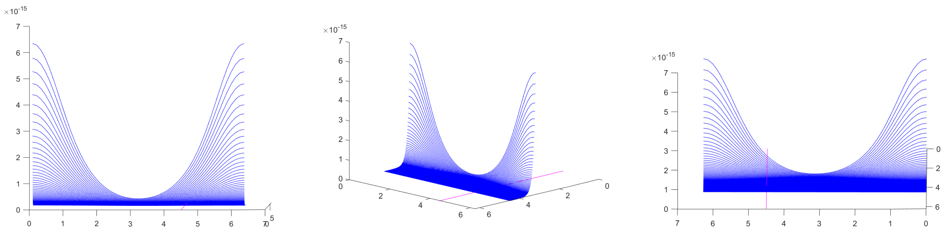
displays the error bounds, $r_n\left(f\right)$, and the actual errors, Error, corresponding to the quadrature rules (3) with the Jacobi weight function. Similarly, Figure 1 presents the modulus of the kernel $\left|K_{n+1,a,b}^{AG}\left(z\right)\right|$. The moduli are computed for $\rho \in [3.8,4.1]$ and for all $\theta \in [0,2\pi ]$. It is evident that the modulus of the kernel attains its maximum value at $\theta =\pi$, as stated in Theorem 1.

Some values of the maxima of the modulus are given; for instance, if ${\rho }_n^{*}=3.8$, then $\left|K_{11,3,1}^{AG}\left(z\right)\right|=2.8909(-12)$, while when ${\rho }_{opt}=15.76$, we have $\left|K_{11,3,1}^{AG}\left(z\right)\right|=3.3046(-24).$

For fixed $n=15,a=-0.5,$ and $b=2,$ 

Table 2. Error bounds $r_n\left(f\right)$ and actual errors for $a=-0.5,b=2$.

n	${\mathit{r}}_{\mathit{n}},\mathit{w}=4$	Error	${\mathit{r}}_{\mathit{n}},\mathit{w}=10$	Error
5	1.8186 (−7)	1.7521 (−9)	6.9455 (−12)	3.7518 (−12)
10	2.1098 (−15)	1.2066 (−16)	5.1631 (−24)	1.2754 (−24)
15	2.2779 (−26)	9.1015 (−28)	4.9495 (−36)	1.1516 (−37)
20	2.3001 (−35)	7.0554 (−37)	2.5942 (−48)	1.0692 (−50)
25	5.6548 (−44)	5.5337 (−46)	1.2840 (−61)	1.0011 (−63)

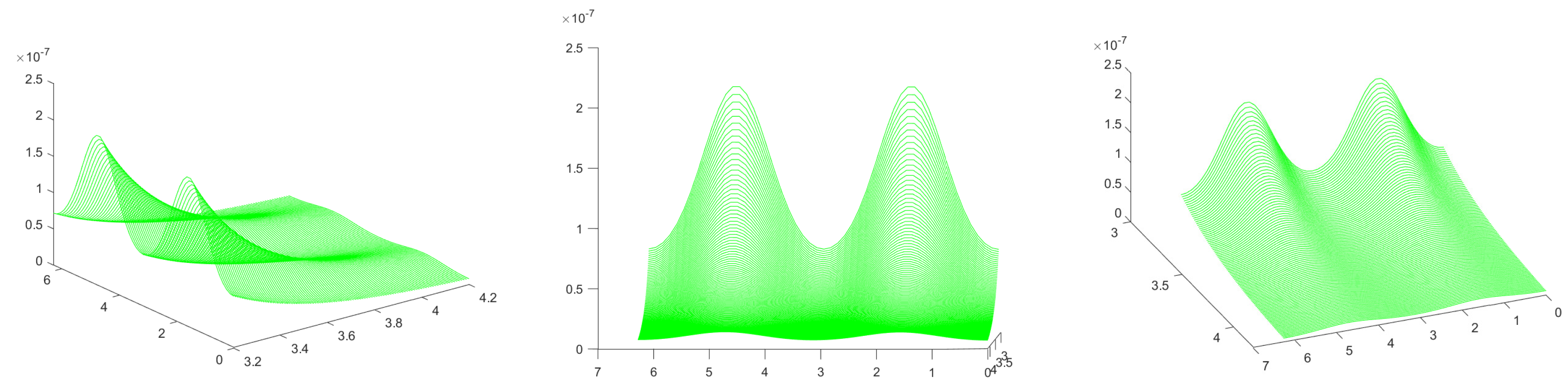
displays the error bounds, $r_n\left(f\right)$, and the actual errors, Error, corresponding to the anti-Gauss quadrature rules. Similarly, Figure 2 represents the modulus of the kernel computed for $\rho \in [3.2,4.5]$ and all $\theta \in [0,2\pi ]$. It is clear that the modulus of the kernel attains its maximum value at $\theta =0$ (i.e., $\theta =2\pi$), as stated in Theorem 1.

Similarly, for the Gegenbauer case, Figure 3 shows that the maximum value is achieved at $\theta ={\displaystyle \frac{\pi }{2}}$ in the case where $n=5$ and $a=b=7$, as predicted by Theorem 2, while

Table 3. Error bounds $r_n\left(f\right)$ and actual errors for $a=7,b=7$.

n	${\mathit{r}}_{\mathit{n}},\mathit{w}=4$	Error	${\mathit{r}}_{\mathit{n}},\mathit{w}=10$	Error
5	6.2545 (−9)	1.7636 (−11)	9.9281 (−14)	8.1560 (−14)
10	3.0964 (−19)	4.1054 (−21)	9.2312 (−27)	3.4202 (−27)
15	1.9454 (−28)	1.7246 (−30)	5.0692 (−39)	1.6879 (−40)
20	1.3866 (−38)	9.2523 (−40)	1.9336 (−51)	1.0685 (−53)
25	5.1204 (−40)	5.6328 (−43)	3.3787 (−64)	7.6894 (−67)

displays the error bounds and the actual errors for the same case.

5. Conclusions

In the current paper, we have obtained sharp bounds for the sup-norm of the kernel in the integral formula for the remainder term of anti-Gauss quadrature rules in the case of Jacobi weight functions. In turn, these bounds have been applied to estimate this remainder term (quadrature error) for an integrand often used in the literature. Both the numerical and the graphical results show the accuracy of the theoretical results.