Abstract
In this paper, we propose a numerical method for the fractional Bagley–Torvik equation of variable coefficients with Robin boundary conditions. The problem is approximated using a finite difference scheme on a uniform mesh that combines the L1 scheme with central differences. We prove that this numerical method is almost first-order convergent. The error bounds for the numerical approximation are derived. The numerical calculations carried out for the given examples validate the theoretical results.
Keywords:
Bagley–Torvik equation; Caputo fractional derivative; Robin boundary conditions; minimum principle; finite difference scheme; L1 scheme MSC:
34A08; 26A33; 35B50; 65L12; 65L20
1. Introduction
Many physical processes of stochastic transport, cellular systems, diffusion waves, control theory [1], signal processing, and the oil industries [2] include fractional-order boundary value problems. In [3], the Bagley–Torvik equation was initially developed to investigate the behavior of real materials using fractional calculus. It may also be used to represent the motion of a rigid plate submerged in a Newtonian fluid, as well as the motion of a gas in a fluid [4].
In [5,6], the authors discussed the existence and uniqueness of a solution for the Bagley–Torvik equation with boundary conditions. H. M. Wei et al. [7] discussed the uniqueness of a solution for fractional Bagley–Torvik equations with variable coefficients.
Many authors have investigated the Bagley–Torvik fractional differential equation to develop methods for numerical solution. These methods are the Adomian decomposition method [4], collocation-shooting method [5], hybridizable discontinuous Galerkin methods [8,9], the wavelet method [10], and the fast multiscale algorithm [11]. Ref. [12] employed a direct piecewise polynomial collocation method to solve the Bagley–Torvik equation. The authors established global convergence results on graded meshes and derived pointwise error estimates on uniform meshes. The authors of [13,14,15] solved the Bagley–Torvik equations with various numerical methods.
S. Santra and J. Mohapatra [16] considered a time-fractional initial boundary value problem of mixed parabolic–elliptic type. Mainly, they used the classical L1 scheme to approximate the temporal derivatives on a uniform mesh and a second-order standard finite difference scheme to approximate the spatial derivatives. The L1 scheme is also used for the Caputo fractional derivative for solving fractional-order Volterra integro-differential equations in Mohapatra et al. [17]. Refs. [18,19,20] used the numerical methods to solve differential equations and integro-differential equations. Gracia et al. [21] investigated the convergence analysis of a time-fractional convection–diffusion problem, where they used the L1 scheme on a uniform mesh. J. Mohapatra et al. [15] utilized L1 discretization on a uniform mesh to approximate the differential operator, and the modified Newton–Raphson method is applied to convert the fractional model into a system of nonlinear algebraic equations. G. Saini et al. [22] discretize the non-local differential operator utilizing a recognized L1 technique, deriving a nonlinear difference equation that encapsulates the fundamental dynamics of the continuous problem. The associated nonlinear equation is resolved using the Daftardar-Gejji and Jafari (DGJ) method. Ghosh, B. and Mohapatra, J. [23] discretize the fractional differential operator employing the conventional L1 method on a uniform mesh, utilizing the composite trapezoidal rule for the integral component. The Daftardar–Gejji and Jafari approach is utilized to resolve the implicit algebraic equation.
Recently, the authors in [24,25] worked on an generalized piecewise Taylor-series expansion method for the generalized Bagley–Torvik equation with a fractional integral and three-point boundary conditions. These authors focused on the fractional Bagley–Torvik equation with variable coefficients. In this article, we propose a finite difference method for the fractional Bagley–Torvik equation of variable coefficients with Robin boundary conditions. The classical L1 scheme is used to approximate the Caputo fractional derivative. To approximate the second-order derivative, a second order central difference scheme is used. We examine the order of convergence on a uniform mesh of the proposed numerical method.
To highlight the novelty and relevance of our study, we summarize the main contributions as follows:
- We propose a finite difference method for solving the fractional Bagley–Torvik equation with variable coefficients subject to Robin boundary conditions. This type of equation arises in viscoelasticity and structural dynamics and poses computational challenges due to the presence of both integer and fractional derivatives.
- To approximate the Caputo fractional derivative, we employ the classical L1 scheme, which is known for its simplicity and effectiveness in handling weakly singular kernels.
- The second-order spatial derivative is discretized using a second-order central difference scheme on a uniform mesh, allowing the method to retain higher accuracy in space while remaining computationally efficient.
- We establish a rigorous convergence analysis of the proposed scheme and show that it achieves almost first-order accuracy in time under standard regularity assumptions on the exact solution.
- Priori error estimates are derived in a discrete norm, which provide theoretical justification for the reliability of the numerical method.
- Several numerical experiments are carried out to confirm the theoretical error bounds and to demonstrate the practical performance of the method. The results show good agreement with the predicted convergence rates, validating both the stability and accuracy of the scheme.
The outline of the paper is as follows: In Section 2, the existence and uniqueness of the solution are proved. Minimum principle, stability result and bounds of solution and its integer derivative are also obtained. The central difference and L1 scheme are constructed for the proposed problem in Section 3. In Section 4, error analysis of this scheme is derived. Three numerical examples are illustrated in Section 5. Finally, the conclusion is presented.
Notations:
- denotes the space of functions, where , ,such that
- C is a positive constant independent of N. We write the maximum norm
- .
2. Continuous Problem
Consider the following fractional Bagley–Torvik equation of variable coefficients with Robin boundary conditions:
where is the differential operator, are sufficiently smooth functions on and
The Caputo fractional derivative of order is defined by
Theorem 1
Proof.
This theorem can be proved by adopting the techniques of the proof of Theorem 2.1 of [26]. □
The operator in (1) satisfies the following minimum principle.
Theorem 2
(Minimum Principle). Let in (1) with , for some . If and then .
Proof.
Define a test function as
Then , and . Further, we define
Suppose the theorem is not true. Then and there exists a point such that and .
Case 1: and . Then,
It is a contradiction.
Case 2: and . Then,
by using Theorem 1 of [27].
It is a contradiction.
Case 3: and . Then,
It is a contradiction. Hence, .
□
Theorem 3
(Stability Result). The solution satisfies the bound
Proof.
Define the barrier functions , where .
Then,
Then by the Theorem 2, we get
□
Corollary 1.
Let for some and with . Then the problem (1) possesses atmost one solution such that ,
where C is a constant.
3. Discrete Problem
The uniform mesh is constructed by dividing into N subintervals. We define the uniform mesh as:
The mesh width is given by .
Consider the following finite difference scheme for the problem (1):
where,
is the L1 discretization of the Caputo fractional derivative [29] defined as
with .
Note: Using the mean value theorem, we can prove
Theorem 4
(Discrete Minimum Principle). Suppose a mesh function satisfies Then .
Proof.
The test function is defined as
Note that .
Define
Assume the theorem is not true. Then and there exists such that and .
Case 1: Assume that for .
Then,
This is a contradiction.
Case 2: Assume that for .
Therefore,
This is a contradiction.
Case 3: Assume that for .
Then,
This is a contradiction. Hence, □
Theorem 5
(Discrete Stability Result). If is a solution of the problem (4) then
Proof.
Define the mesh functions
We have and . Using Theorem 4, the result can be proved. □
4. Error Analysis
4.1. Local Truncation Error
Let us consider the local truncation error of the problem (4):
Lemma 1.
Suppose for some and . Then the truncation error bound satisfies
Proof.
Using Corollary 1 yields
Now,
Consider,
Case (i): If
from Corollary 1.
Case (ii): If ,
where we used Corollary 1 and
Using remark 2 of [30], we get
From the bound of and , we get the desired result. □
4.2. Error Estimate
Theorem 6.
Proof.
Define the mesh functions
Then, we have
By the L1 discretization of Caputo fractional derivative and (5), we get
Therefore
Applying Theorem 4, we get
Hence, it is proved. □
5. Numerical Exemplifications
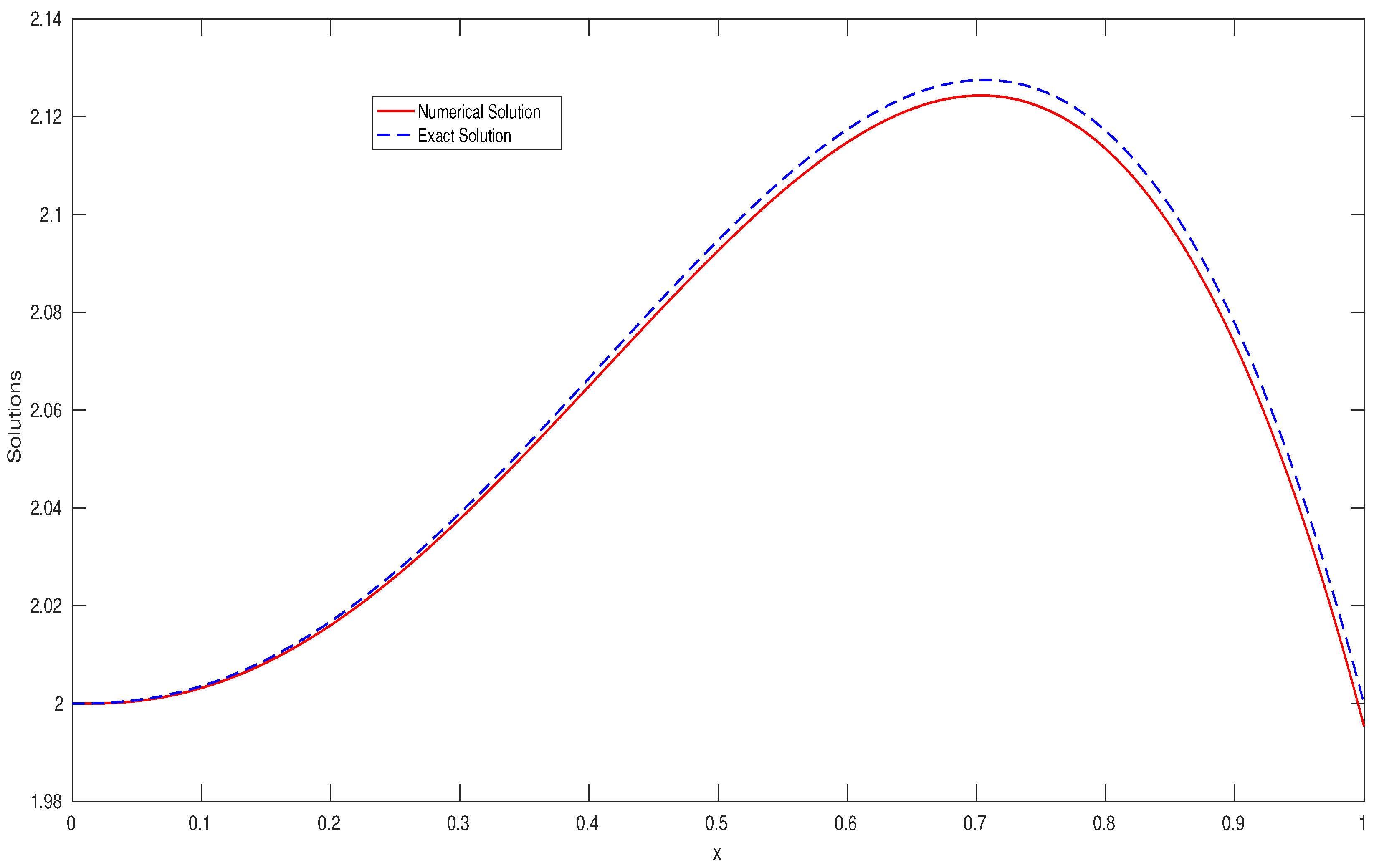
Example 1.
The exact solution is , where the function and the constants A and B are chosen using . We evaluate the maximum pointwise error and rate of convergence by
Uniform errors for the various values of and the corresponding rate of convergence are obtained by
The numerical solution and exact solution of Example 1 are plotted in Figure 1.
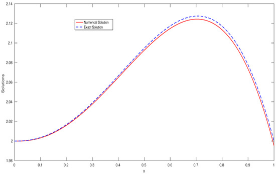
Figure 1.
Exact and approximate solutions of Example 1 for and .
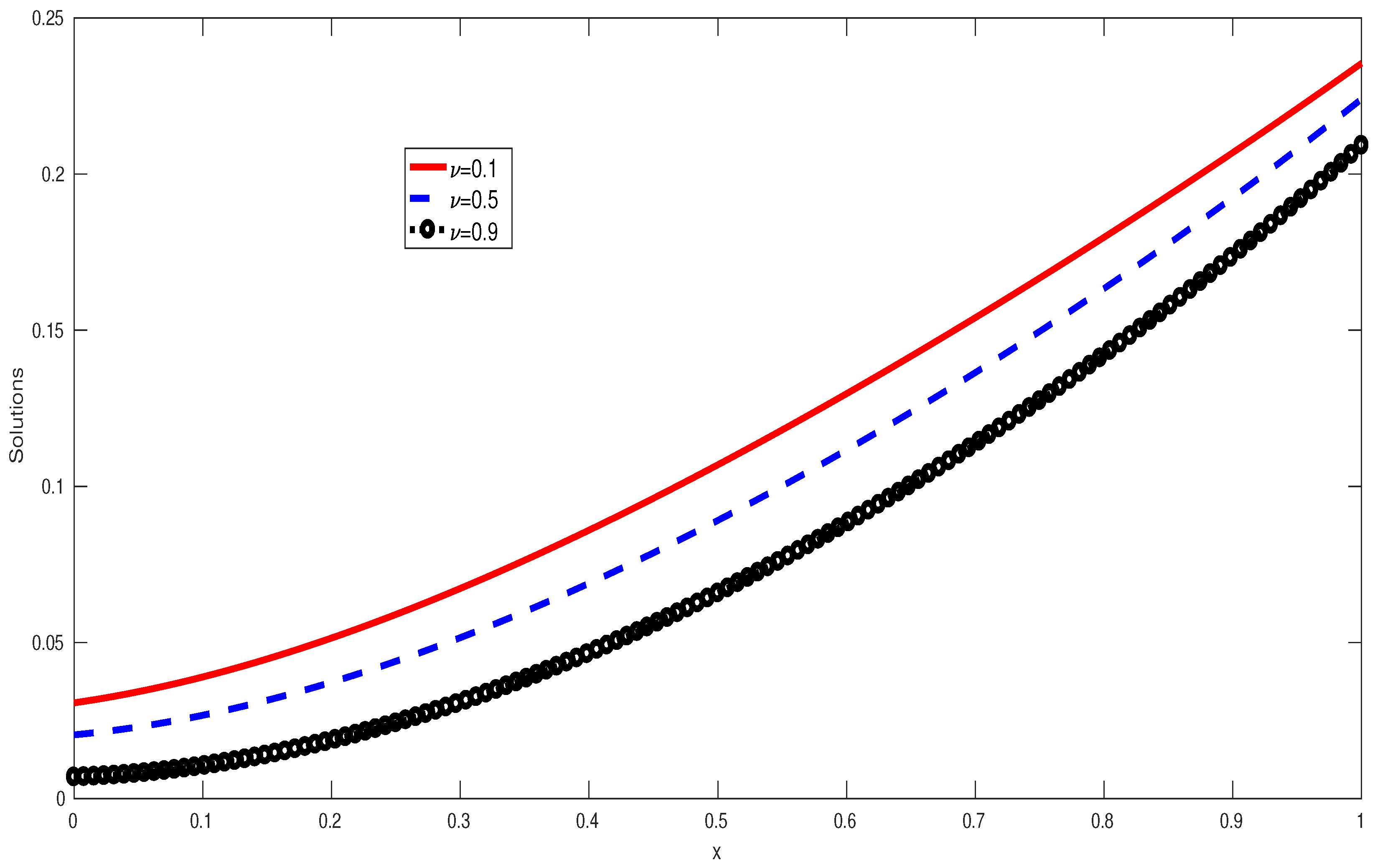
Example 2.
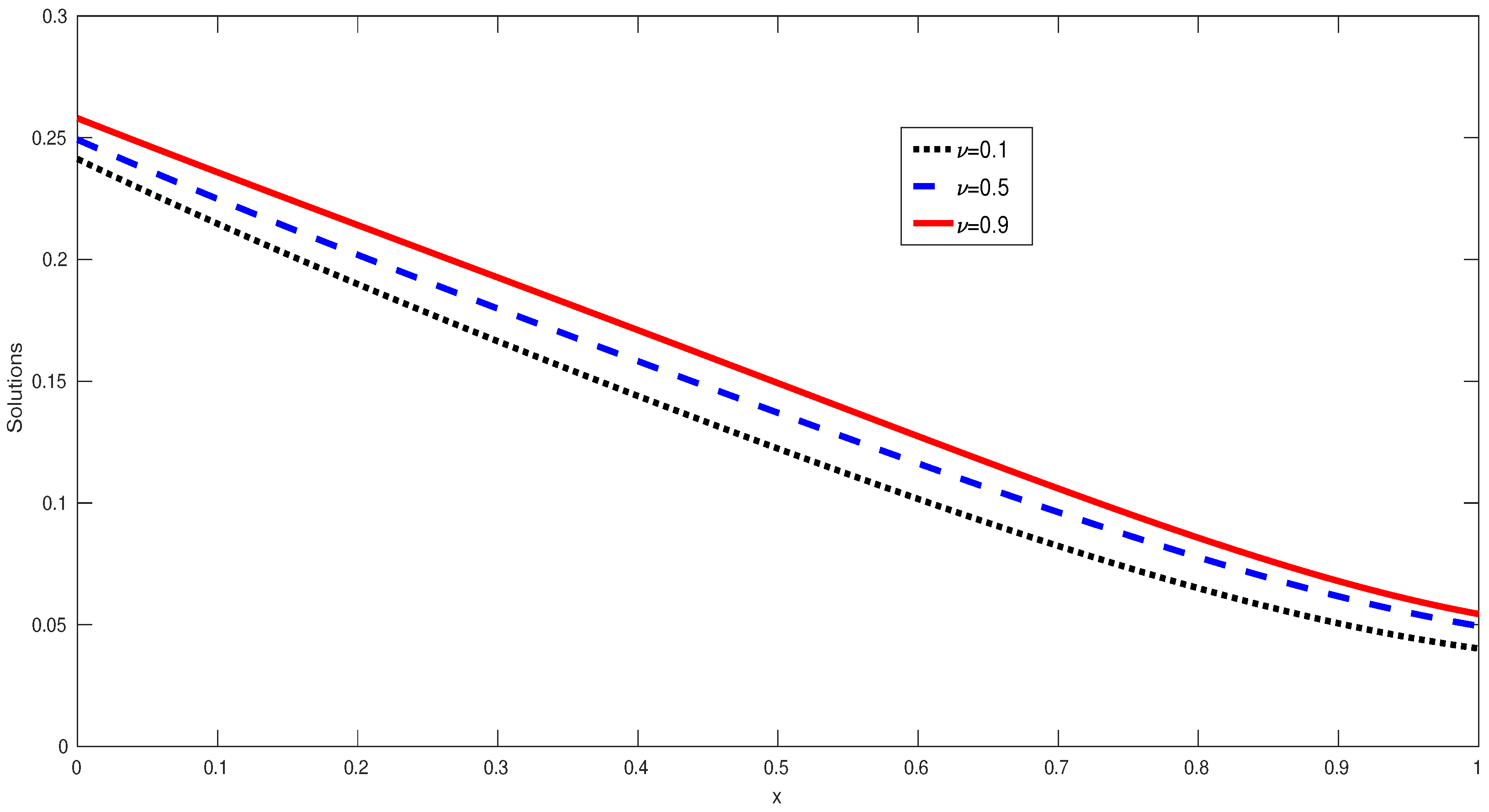
Example 3.
The exact solutions to Examples 2 and 3 are unknown. Table 1 and Table 2 show the maximum pointwise errors and uniform rates of convergence which are obtained by using the double mesh principle [31] defined as follows:
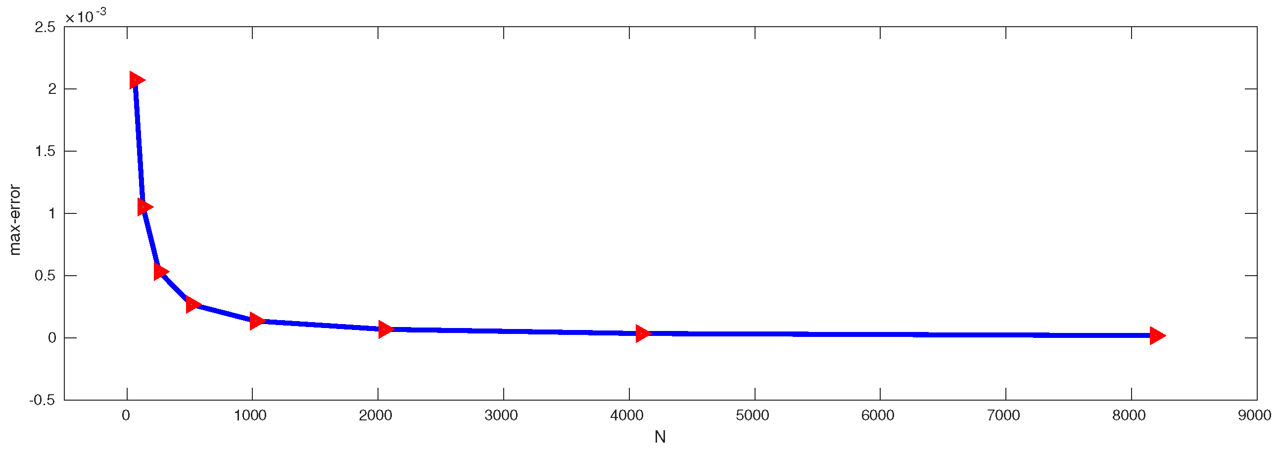
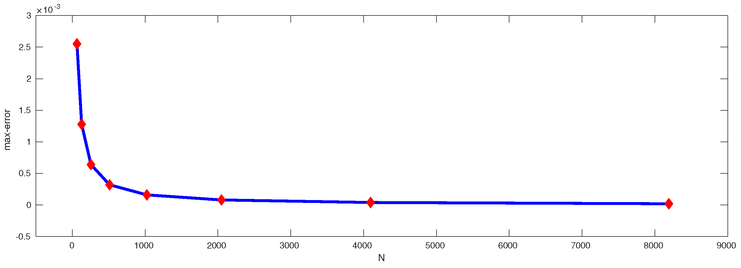
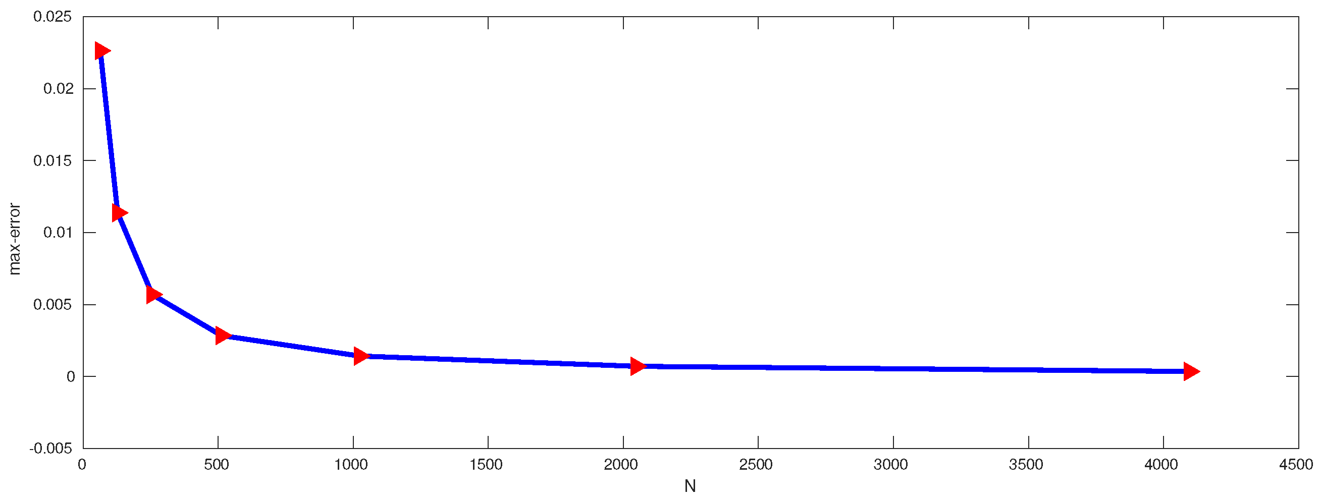
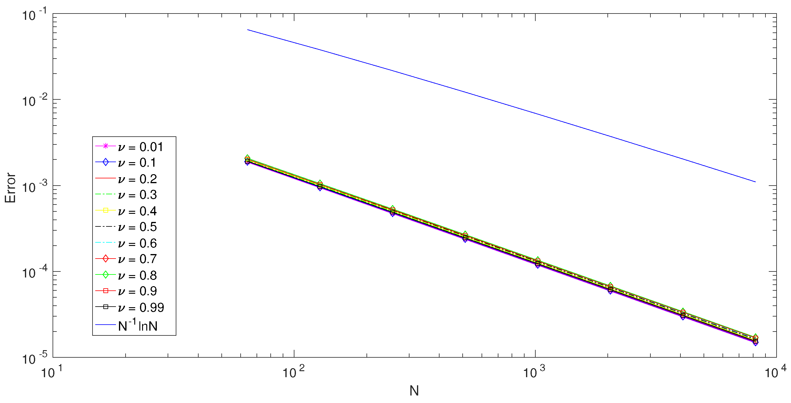
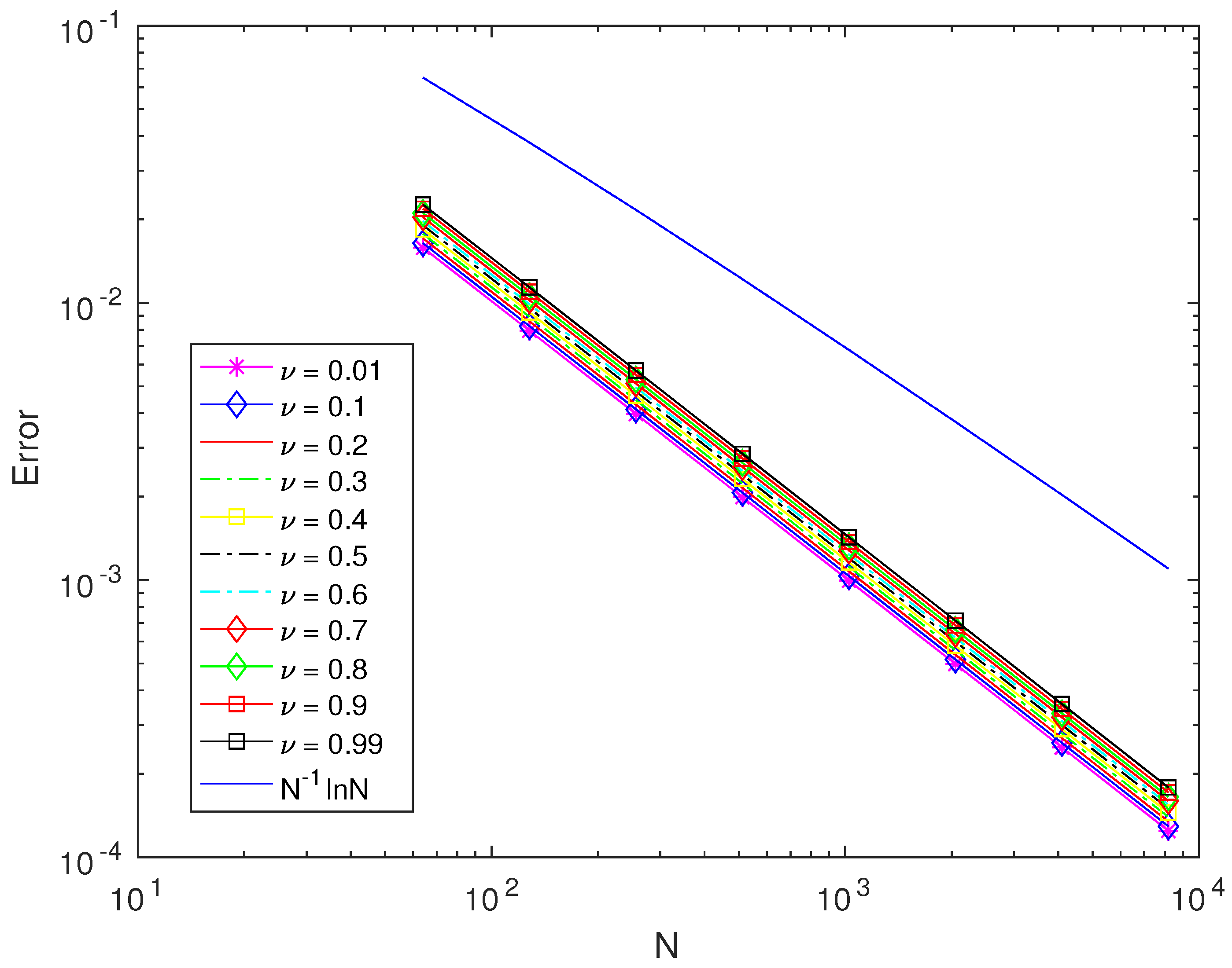
The numerical solution of Examples 2 and 3 are plotted in Figure 2 and Figure 3. The error plot in Figure 4, Figure 5 and Figure 6 indicates that as the value of N increases as the maximum errors decreases. Table 1, Table 2 and Table 3 show the uniform errors and convergence orders of Examples 1, 2, and 3, respectively. The loglog plot in Figure 7, Figure 8 and Figure 9 validates our theoritical error bound which is of .

Table 1.
Enumerated maximum errors and uniform errors and orders of convergence of Example 2 for the values of .
Table 2.
Enumerated maximum errors and uniform errors and orders of convergence of Example 3 for the values of .

Figure 2.
The numerical solution for and .
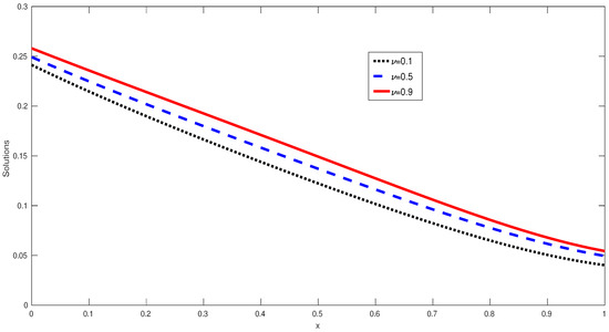
Figure 3.
The numerical solution for and .
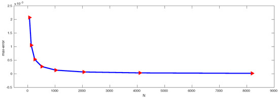
Figure 4.
Error plot for Example 1.
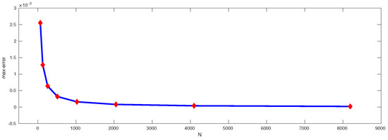
Figure 5.
Error plot for Example 2.
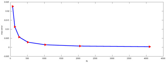
Figure 6.
Error plot for Example 3.
Table 3.
Enumerated maximum errors and uniform errors and orders of convergence of Example 1 for the values of .
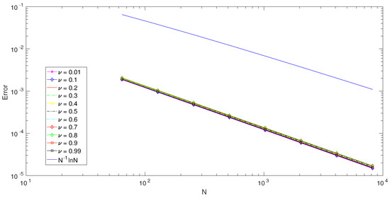
Figure 7.
Log-log plot for Example 1.
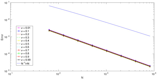
Figure 8.
Log-log plot for Example 2.
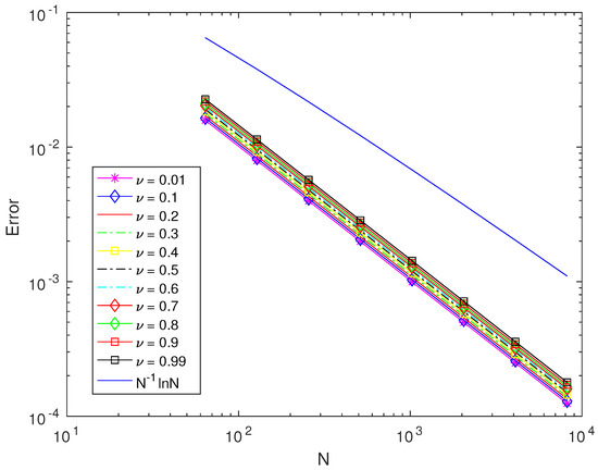
Figure 9.
Log-log plot for Example 3.
6. Conclusions
The proposed finite difference scheme provides an efficient and accurate numerical method for solving the fractional Bagley–Torvik equation with variable coefficients and Robin boundary conditions. The combination of the L1 scheme for the fractional derivative with central difference approximations ensures simplicity in implementation while maintaining stability. Theoretical analysis confirms that the method achieves nearly first-order convergence, and rigorous error bounds are derived. Numerical experiments further validate the analytical results, demonstrating the reliability, accuracy, and practical applicability of the scheme for solving fractional differential equations arising in engineering and applied sciences.
Author Contributions
Validation, R.A.; Formal analysis, M.A.; Writing—original draft, S.J.C.M.; Writing—review & editing, S.E. All authors have read and agreed to the published version of the manuscript.
Funding
This work was supported by the Deanship of Scientific Research, Vice Presidency for Graduate Studies and Scientific Research, King Faisal University, Saudi Arabia. [Grant No.KFU252194]. This study is supported via funding from Prince Sattam bin Abdulaziz University, Saudi Arabia, project number [PSAU/2025/R/1446].
Data Availability Statement
The original contributions presented in this study are included in the article. Further inquiries can be directed to the corresponding author.
Conflicts of Interest
The authors declare that they have no competing interests concerning the publication of the manuscript.
References
- Manabe, S. A suggestion of fractional-order controller for flexible spacecraft attitude control. Nonlinear Dyn. 2002, 29, 251–268. [Google Scholar] [CrossRef]
- Fitt, A.D.; Goodwin, A.R.H.; Ronaldson, K.A.; Wakeham, W.A. A fractional differential equation for a MEMS viscometer used in the oil industry. J. Comput. Appl. Math. 2009, 229, 373–381. [Google Scholar] [CrossRef]
- Bagley, R.L.; Torvik, P.J. A different approach to the analysis of viscoelas- tically damped structures. AIAA J. 1983, 21, 741–748. [Google Scholar] [CrossRef]
- Ray, S.S.; Bera, R.K. Analytical solution of the Bagley—Torvik equation by Adomian decomposition method. Appl. Math. Comput. 2005, 168, 398–410. [Google Scholar] [CrossRef]
- Al-Mdallal, Q.; Syam, M.; Anwar, M.N. A collocation-shooting method for solving fractional boundary value problems. Commun. Nonlinear Sci. Numer. Simul. 2010, 15, 3814–3822. [Google Scholar] [CrossRef]
- Podlubny, I. Fractional Differential Equations; Academic Press: San Diego, CA, USA, 1999. [Google Scholar]
- Wei, H.M.; Zhong, X.C.; Huang, Q.A. Uniqueness and approximation of solution for fractional Bagley—Torvik equations with variable coefficients. Int. J. Comput. Math. 2017, 94, 1542–1561. [Google Scholar] [CrossRef]
- Karaaslan, M.F.; Celiker, F.; Kurulay, M. Approximate solution of the Bagley—Torvik equation by hybridizable discontinuous Galerkin methods. Appl. Math. Comput. 2016, 285, 51–58. [Google Scholar] [CrossRef]
- Izadi, M.; Negar, M.R. Local discontinuous Galerkin approximations to fractional Bagley—Torvik equation. Math. Methods Appl. Sci. 2020, 43, 4798–4813. [Google Scholar] [CrossRef]
- Balaji, S.; Hariharan, G. An efficient operational matrix method for the numerical solutions of the fractional Bagley–Torvik equation using wavelets. J. Math. Chem. 2019, 57, 1885–1901. [Google Scholar] [CrossRef]
- Chen, J. A fast multiscale Galerkin algorithm for solving boundary value problem of the fractional Bagley—Torvik equation. Bound. Value Probl. 2020, 91, 1–13. [Google Scholar] [CrossRef]
- Wang, L.; Liang, H. Analysis of direct piecewise polynomial collocation methods for the Bagley—Torvik equation. Bit. Numer. Math. 2024, 64, 41. [Google Scholar] [CrossRef]
- Wang, L.; Liang, H. Superconvergence and postprocessing of collocation methods for fractional differential equation. J. Sci. Comput. 2023, 97, 29. [Google Scholar] [CrossRef]
- Liang, H.; Stynes, M. A general collocation analysis for weakly singular Volterra integral equations with variable exponent. IMA J. Numer. Anal. 2024, 44, 2725–2751. [Google Scholar] [CrossRef]
- Mohapatra, J.; Mohapatra, S.P.; Anasuya, N. An approximation technique for a system of time-fractional differential equations arising in population dynamics. J. Math. Model. 2025, 13, 519–531. [Google Scholar]
- Santra, S.; Mohapatra, J. Analysis of the L1 scheme for a time fractional parabolic–elliptic problem involving weak singularity. Math. Methods Appl. Sci. 2021, 44, 1529–1541. [Google Scholar] [CrossRef]
- Santra, S.; Mohapatra, J. Numerical analysis of Volterra integro-differential equations with Caputo fractional derivative. Iran J. Sci. Technol. Trans. Sci. 2021, 45, 1815–1824. [Google Scholar] [CrossRef]
- Sekar, E. Second order singularly perturbed delay differential equations with non-local boundary condition. J. Comput. Appl. Math. 2023, 417, 114498. [Google Scholar]
- Elango, S.; Govindarao, L.; Awadalla, M.; Zaway, H. Efficient Numerical Methods for Reaction–Diffusion Problems Governed by Singularly Perturbed Fredholm Integro-Differential Equations. Mathematics 2025, 13, 1511. [Google Scholar] [CrossRef]
- Raja, V.; Sekar, E.; Loganathan, K. Computational approaches for singularly perturbed turning point problems with non-local boundary conditions. Partial Differ. Equ. Appl. Math. 2025, 13, 101122. [Google Scholar] [CrossRef]
- Gracia, J.; O’Riordan, E.; Stynes, M. Convergence in positive time for a finite difference method applied to a fractional convection-diffusion problem. Comput. Methods Appl. Math. 2018, 18, 33–42. [Google Scholar] [CrossRef]
- Saini, G.; Ghosh, B.; Sunita, C.; Mohapatra, J. An iterative-based difference scheme for nonlinear fractional integro-differential equations of Volterra type. Partial Differ. Equ. Appl. Math. 2025, 13, 101138. [Google Scholar] [CrossRef]
- Ghosh, B.; Mohapatra, J. An iterative difference scheme for solving arbitrary order nonlinear Volterra integro-differential population growth model. J. Anal. 2024, 32, 57–72. [Google Scholar] [CrossRef]
- Huang, Q.A.; Zhong, X.C.; Guo, B.L. Approximate solution of Bagley—Torvik equations with variable coefficients and three-point boundary-value conditions. Int. J. Appl. Comput. Math. 2016, 215, 327–347. [Google Scholar] [CrossRef]
- Zhong, X.; Liu, X.; Liao, S.L. On a generalized Bagley–Torvik equation with a fractional integral boundary condition. Int. J. Appl. Comput. Math. 2017, 3, 727–746. [Google Scholar] [CrossRef]
- Pedas, A.; Tamme, E. Piecewise polynomial collocation for linear boundary value problems of fractional differential equations. J. Comput. Appl. Math. 2012, 236, 3349–3359. [Google Scholar] [CrossRef]
- Luchko, Y. Maximum principle for the generalized time-fractional diffusion equation. J. Math. Anal. Appl. 2009, 351, 218–223. [Google Scholar] [CrossRef]
- Stynes, M.; Gracia, J. A finite difference method for a two-point boundary value problem with a Caputo fractional derivative. IMA J. Numer. Anal. 2015, 35, 698–721. [Google Scholar] [CrossRef]
- Li, C.; Zeng, F. Numerical Methods for Fractional Calculus; CRC Press, Taylor & Francis Group: Boca Raton, FL, USA, 2015. [Google Scholar]
- Gracia, J.; O’Riordan, E.; Stynes, M. Convergence outside the initial layer for a numerical method for the time-fractional heat equation. In International Conference on Numerical Analysis and Its Applications; Springer International Publishing: Cham, Switzerland, 2016. [Google Scholar]
- Farrell, P.A.; Hegarty, A.F.; Miller, J.J.H.; O’Riordan, E.; Shishkin, G.I. Robust Computational Techniques for Boundary Layers; Applied Mathematics; Chapman & Hall/CRC: Boca Raton, FL, USA, 2000. [Google Scholar]

Disclaimer/Publisher’s Note: The statements, opinions and data contained in all publications are solely those of the individual author(s) and contributor(s) and not of MDPI and/or the editor(s). MDPI and/or the editor(s) disclaim responsibility for any injury to people or property resulting from any ideas, methods, instructions or products referred to in the content. |
© 2025 by the authors. Licensee MDPI, Basel, Switzerland. This article is an open access article distributed under the terms and conditions of the Creative Commons Attribution (CC BY) license (https://creativecommons.org/licenses/by/4.0/).