
Carbon Dioxide Emission Forecasting Using BiLSTM Network Based on Variational Mode Decomposition and Improved Black-Winged Kite Algorithm


Abstract
1. Introduction
- The variational mode decomposition method is applied to carbon dioxide emission prediction, incorporating the nonlinear characteristics of sample data, with the aim of mitigating the impact of inherent non-stationarity in raw data on forecasting accuracy. This approach has significantly enhanced prediction precision and provides a novel perspective for the exploration of carbon dioxide emission forecasting.
- A VMD-IBKA-BiLSTM framework is proposed for carbon dioxide emission prediction, where BiLSTM is established as a deep learning model specifically designed for carbon dioxide emission forecasting, and IBKA is formulated as an enhanced BKA algorithm dedicated to hyperparameter optimization of BiLSTM.
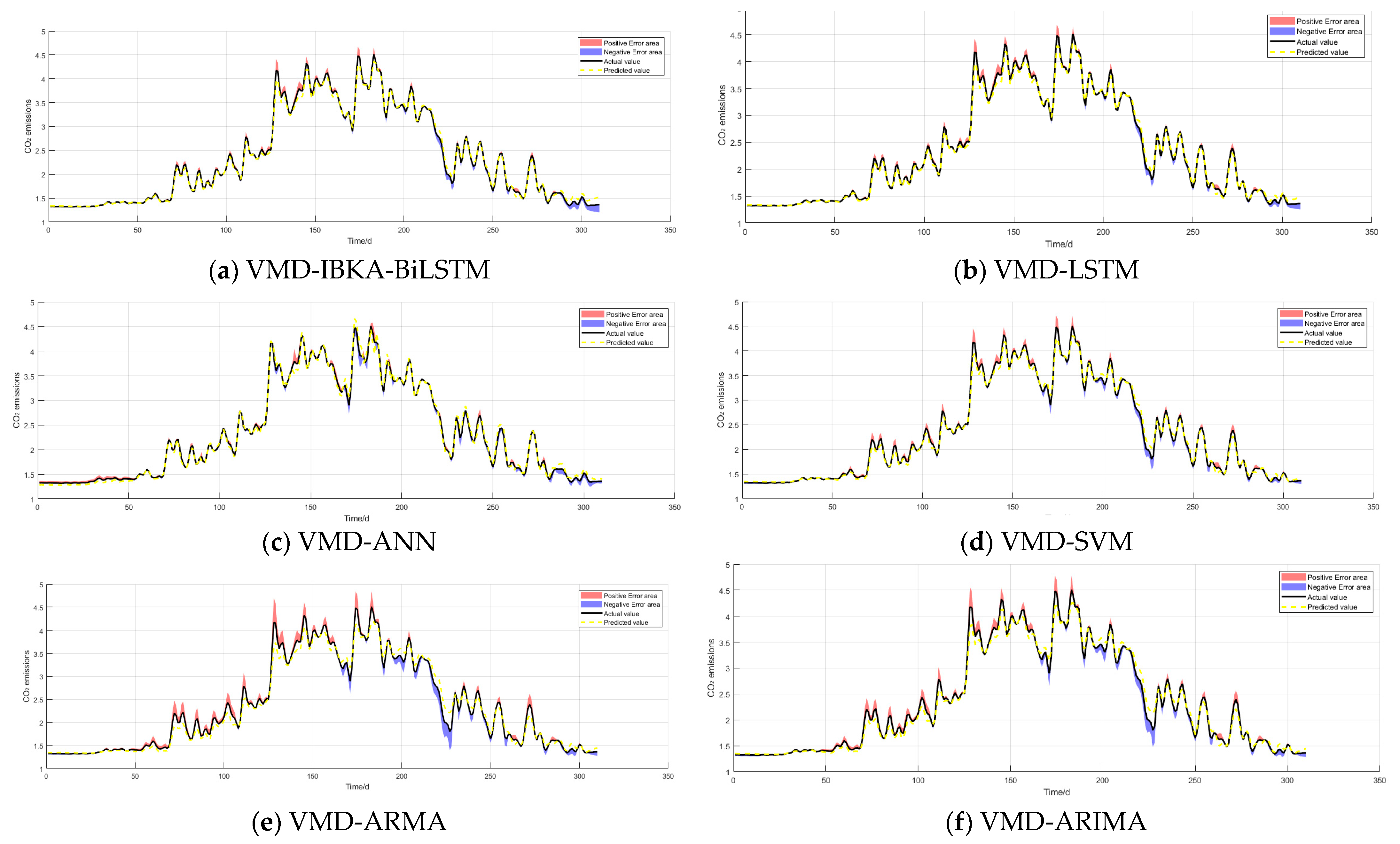
- The VMD-IBKA-BiLSTM model proposed in this study was comparatively evaluated against models ARMA, ARIMA, SVM, ANN, and LSTM in predicting carbon dioxide emissions from four sectors in China. The results demonstrate that significant superiority of the proposed model over the comparative models is observed.
2. Materials and Methods
2.1. VMD
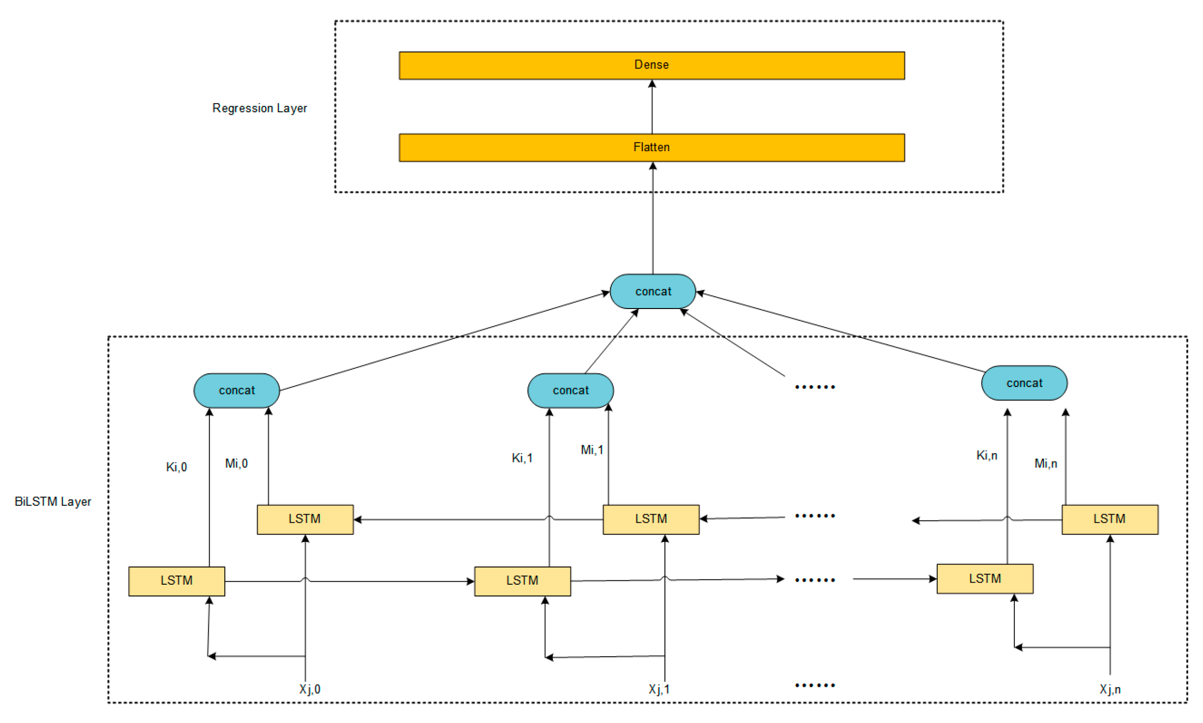
2.2. Carbon Dioxide Emission Forecasting Model: BiLSTM
2.3. IBKA
2.3.1. The Original BKA
- 1.
- Population initialization phase
- 2.
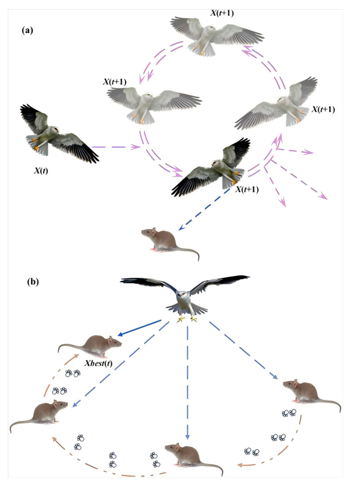
- Aggressive behavior
- and represent the position of the i-th black-winged kite in the j-th dimension at the t-th and (t + 1)th iteration steps, respectively.
- r is a random number between 0 and 1, while p is a constant value equal to 0.9.
- T is the total number of iterations, and t is the number of iterations that have been completed.
- n is the dynamic perturbation coefficient.
- 3.
- Migration behavior
- represents the leading scorer in the j-th dimension for the black-winged kite at the t-th iteration so far.
- and represent the position of the i-th black-winged kite in the j-th dimension at the t-th and (t + 1)th iteration steps, respectively.
- represents the current position of any black-winged kite in the j-th dimension at the t-th iteration.
- represents the fitness value of the random position in the j-th dimension obtained from any black-winged kite at the t-th iteration.
- C (0,1) represents Cauchy mutation. It is defined as follows:
2.3.2. Proposed IBKA
- 1.
- Lévy Flight-Inspired Prey Escape and Collective Cooperation Strategies
- 2.
- Nonlinear Simplex Strategy
3. Results and Discussion
3.1. IBKA Performance Verification Experiments
3.1.1. Benchmark Functions
3.1.2. Ablation Analysis of the IBKA
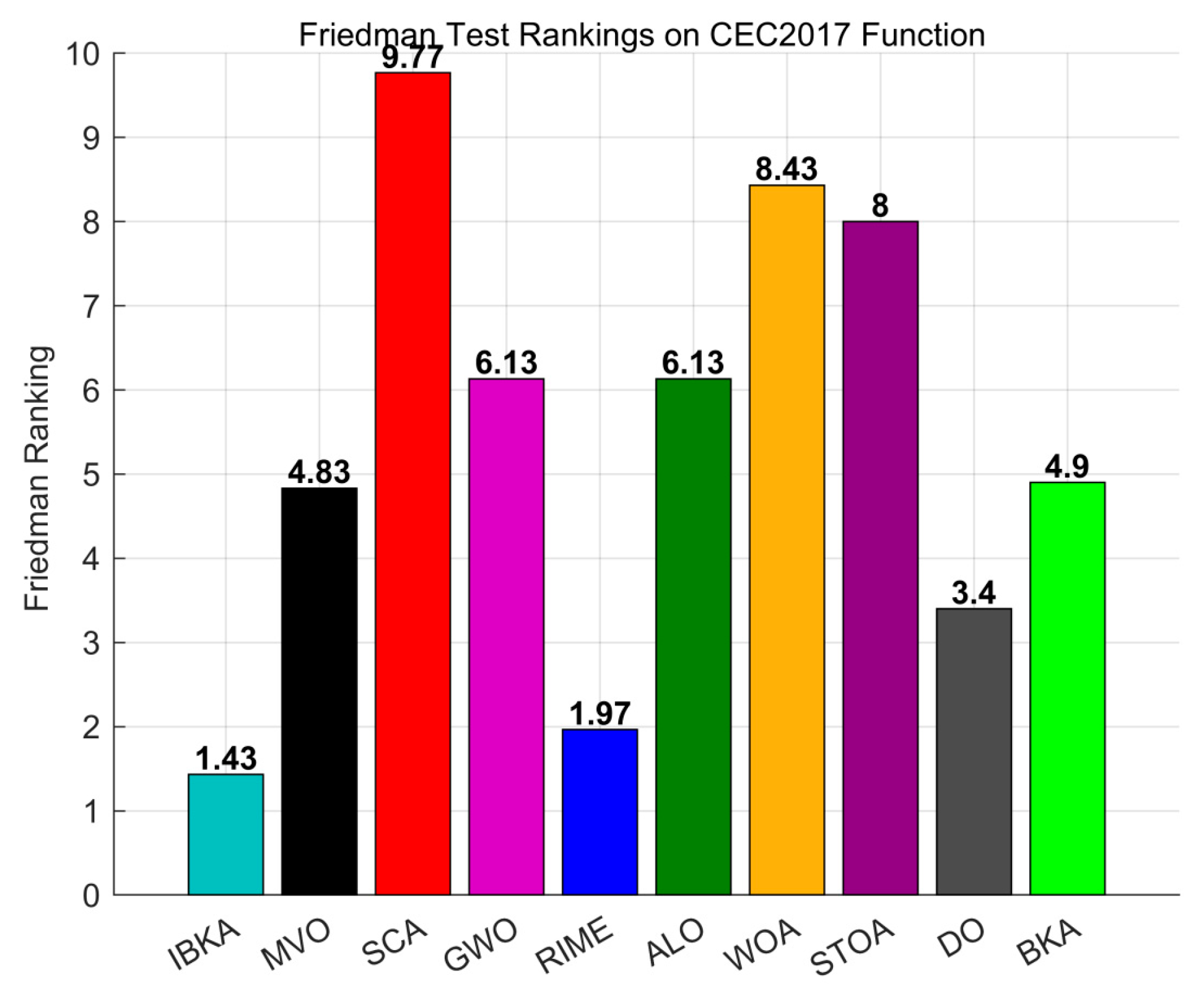
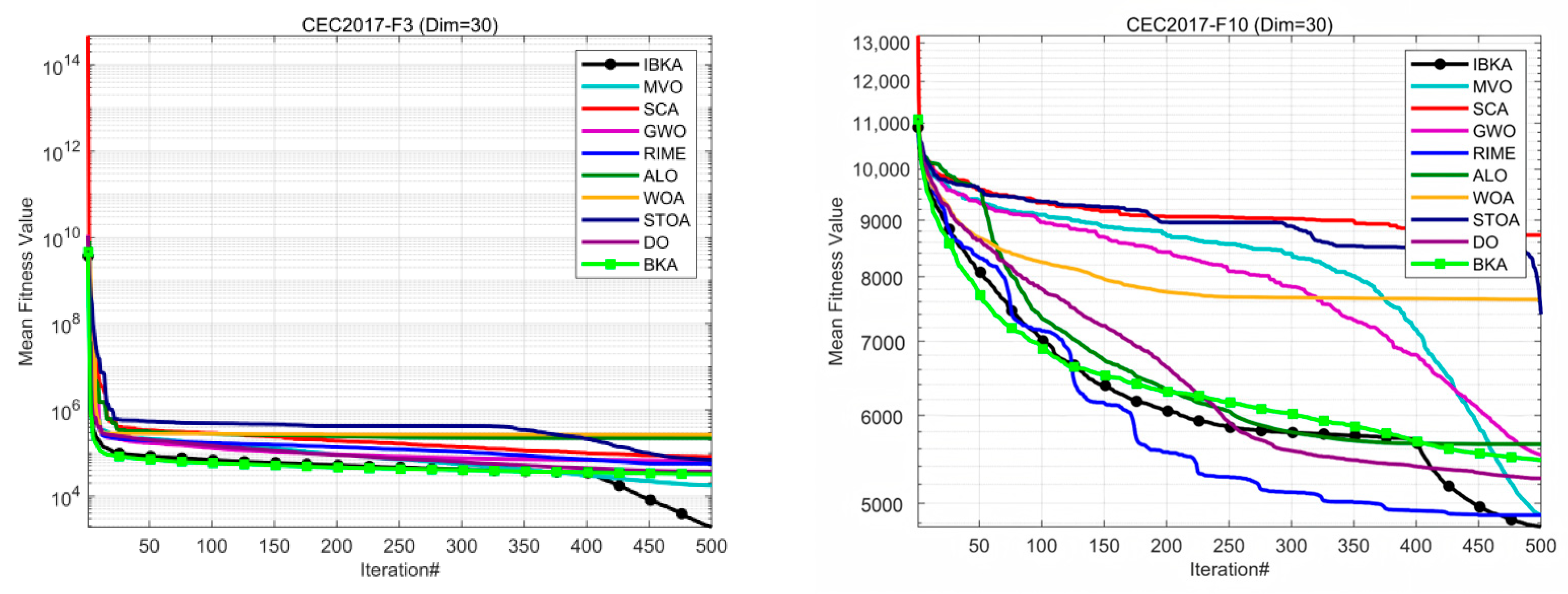
3.1.3. Comparison with Other Algorithms
- Multi-verse optimization algorithm (MVO) [38]
- Sine cosine algorithm (SCA) [39]
- Grey wolf optimization (GWO) [40]
- Rime optimization algorithm (RIME) [41]
- Ant lion optimization (ALO) [42]
- The whale optimization algorithm (WOA) [43]
- Sooty tern optimization algorithm (STOA) [44]
- Dandelion optimization (DO) [45]
- Black-winged kites algorithm (BKA) [48]
3.2. VMD-IBKA-BiLSTM Framework for CO2 Emission Forecasting
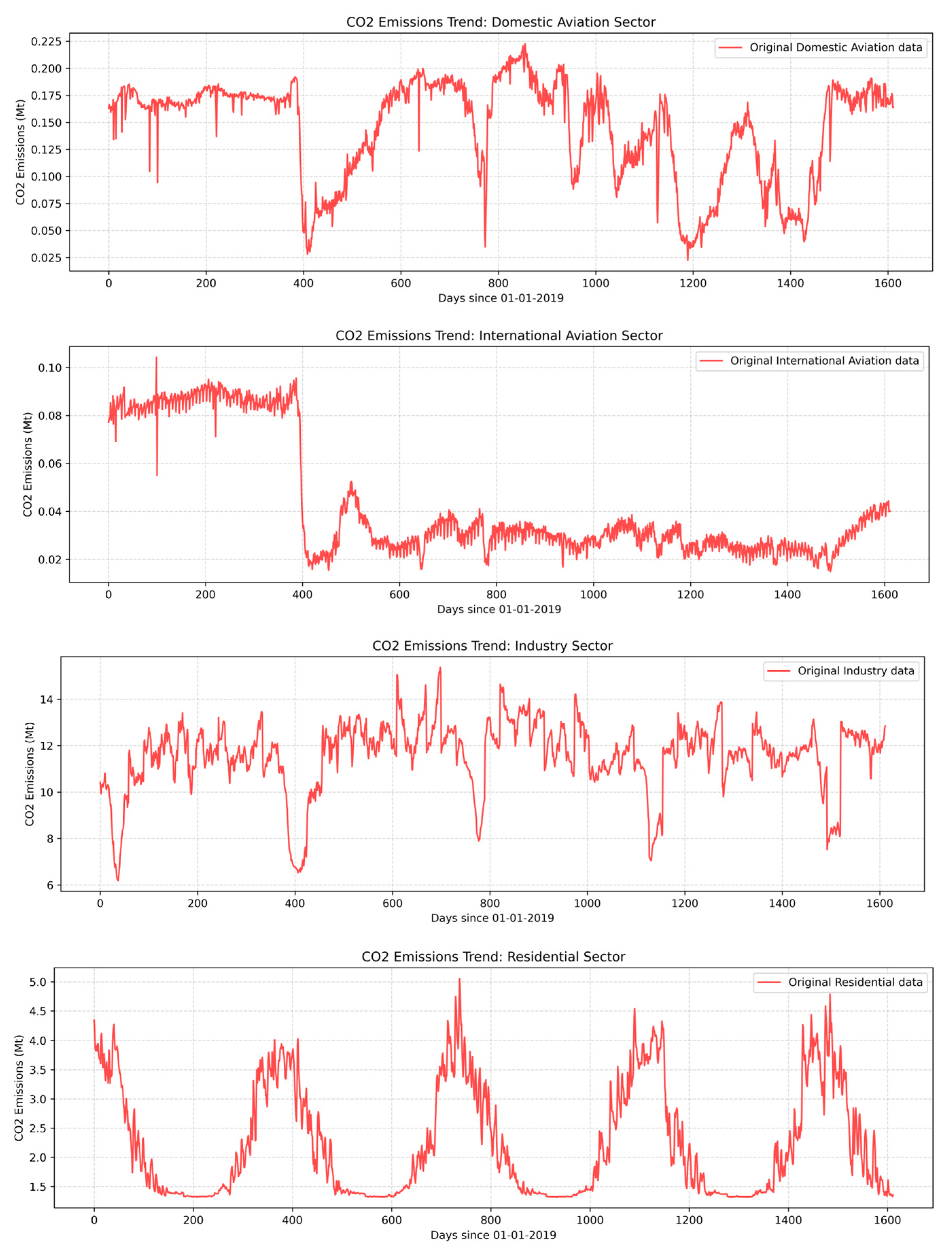
3.2.1. CO2 Emission Data
3.2.2. VMD Parameters
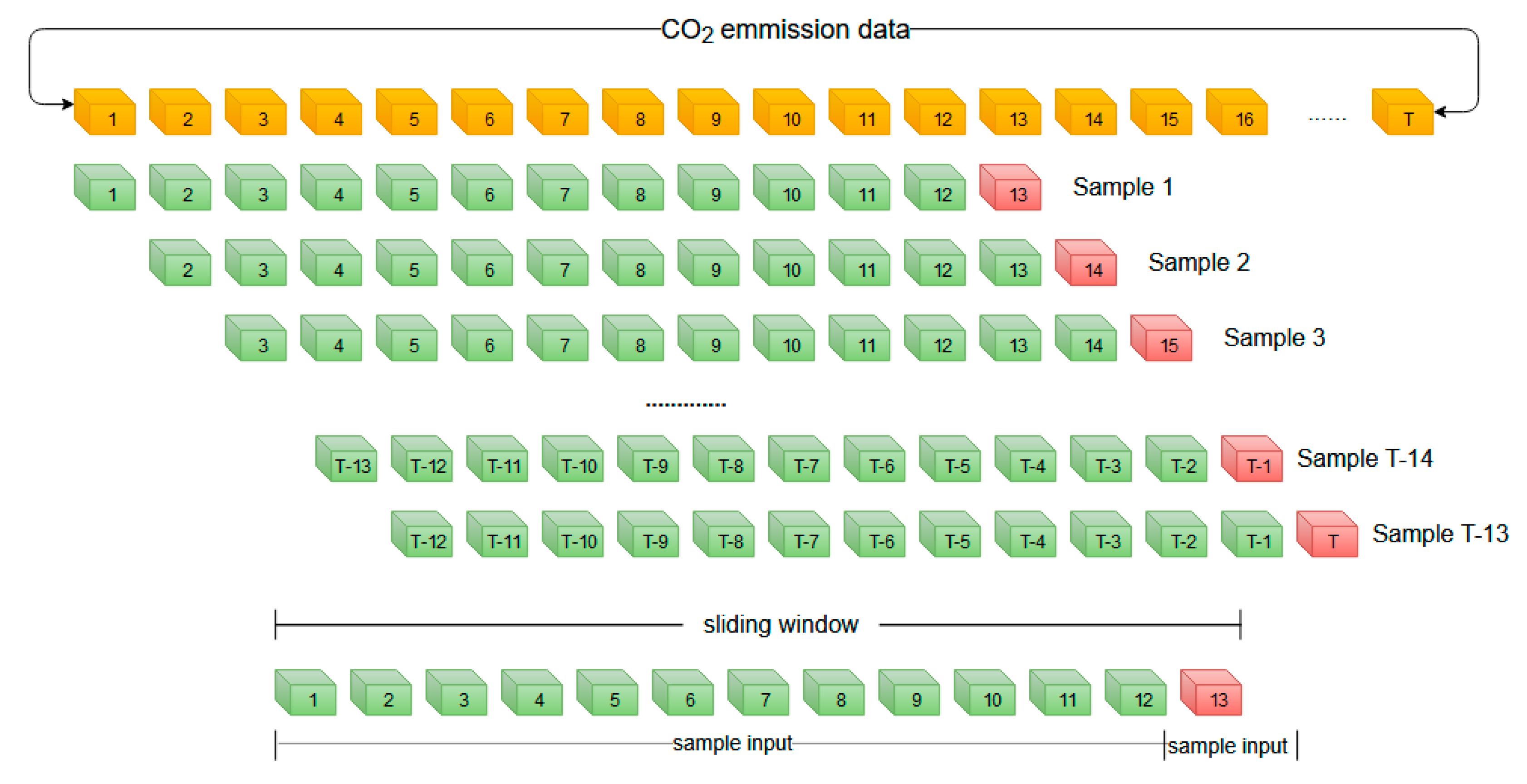
3.2.3. Sample Making
3.2.4. VMD-IBKA-BiLSTM Flowchart

| Hyperparameter Name | Description | Lower Bounds | Upper Bounds |
|---|---|---|---|
| unit | The number of units in the BiLSTM layer | 50 | 300 |
| learning_rate | Parameter update step during model training | 0.001 | 0.01 |
| max_epochs | Maximum number of cycles for model training | 50 | 300 |
3.2.5. Evaluation Metrics
3.2.6. Comparison of BiLSTM Optimized by Various Algorithms
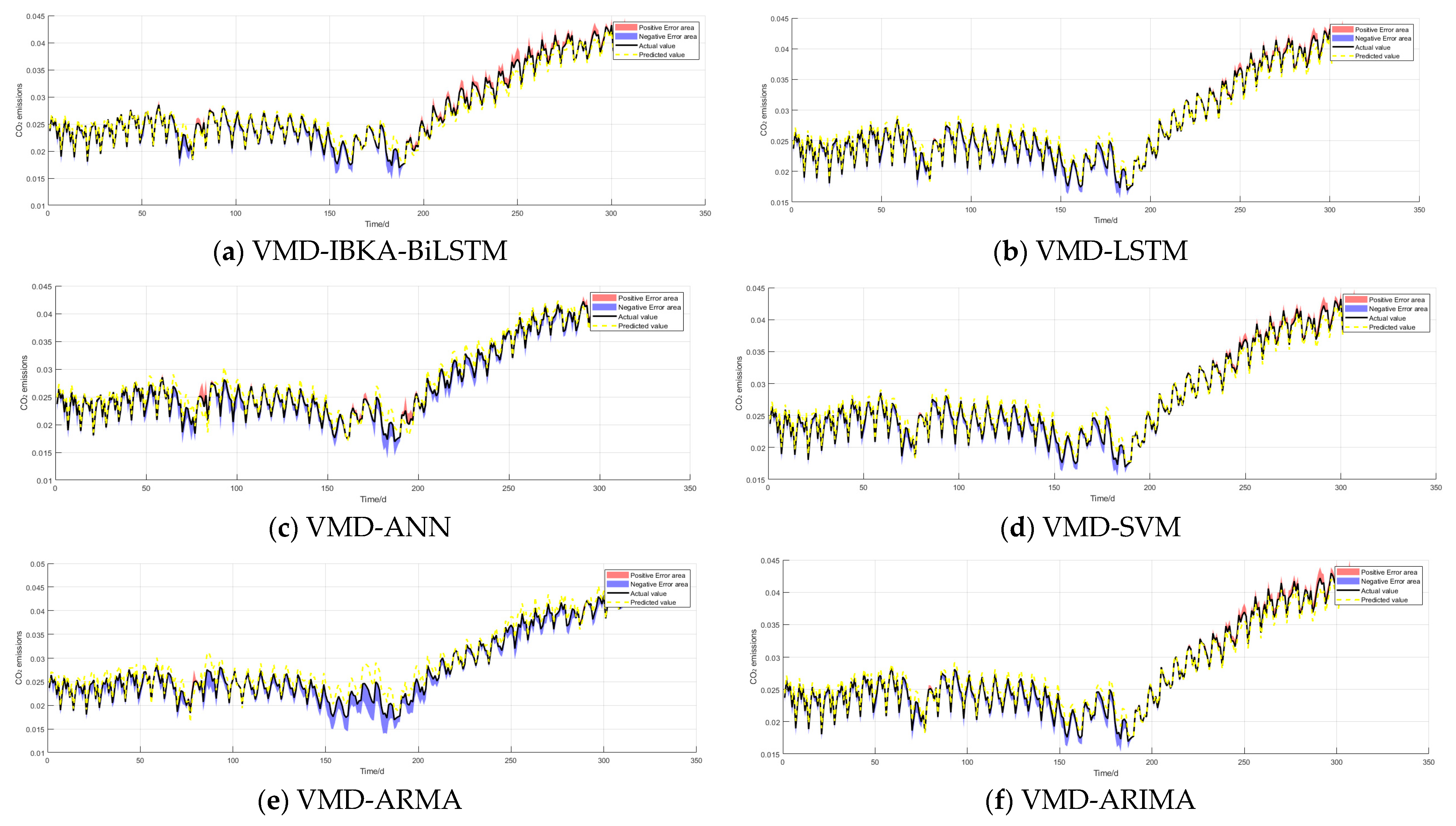
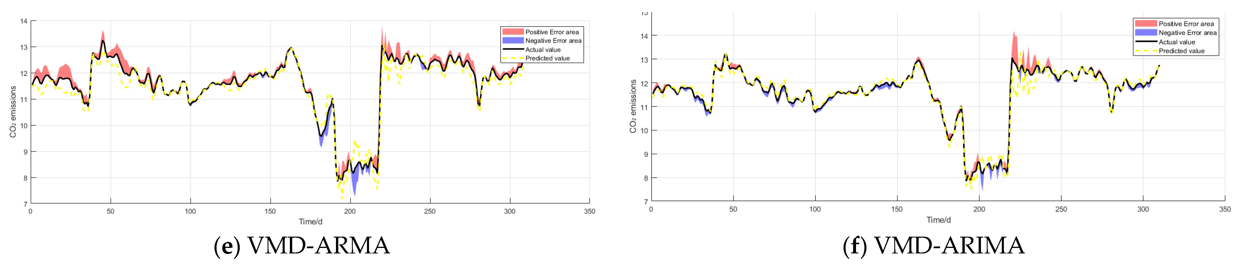
3.2.7. Comparison with Other Models
4. Conclusions
Author Contributions
Funding
Data Availability Statement
Acknowledgments
Conflicts of Interest
References
- Alizadeh, O. A review of ENSO teleconnections at present and under future global warming. Wiley Interdiscip. Rev. Clim. Change 2024, 15, e861. [Google Scholar] [CrossRef]
- Mehmood, K.; Tauseef Hassan, S.; Qiu, X.; Ali, S. Comparative analysis of CO2 emissions and economic performance in the United States and China: Navigating sustainable development in the climate change era. Geosci. Front. 2024, 15, 101843. [Google Scholar] [CrossRef]
- Zhang, Z.; Wang, G. China’s role in global climate governance. Clim. Policy 2017, 17 (Suppl. S1), 32–47. [Google Scholar]
- IEA. An Energy Sector Roadmap to Carbon Neutrality in China. Energy Technology Policy Division; IEA: Paris, France, 2021. [Google Scholar]
- MEE. List of Chemicals Under Priority Control (Second Batch); Ministry of Ecology and Environment of the People’s Republic of China: Beijing, China, 2020. [Google Scholar]
- Benoit, K. Linear Regression Models with Logarithmic Transformations; London School of Economics: London, UK, 2011; Volume 22, pp. 23–36. [Google Scholar]
- De Livera, A.M.; Hyndman, R.J.; Snyder, R.D. Forecasting time series with complex seasonal patterns using exponential smoothing. J. Am. Stat. Assoc. 2011, 106, 1513–1527. [Google Scholar] [CrossRef]
- Ge, H.; Chen, G.; Yu, H.; Chen, H.; An, F. Theoretical analysis of empirical mode decomposition. Symmetry 2018, 10, 623. [Google Scholar] [CrossRef]
- Faysal, A.; Ngui, W.K.; Lim, M.H. Noise eliminated ensemble empirical mode decomposition for bearing fault diagnosis. J. Vib. Eng. Technol. 2021, 9, 2229–2245. [Google Scholar] [CrossRef]
- Dragomiretskiy, K.; Zosso, D. Variational mode decomposition. IEEE Trans. Signal Process. 2013, 62, 531–544. [Google Scholar] [CrossRef]
- Ahmadi, F.; Tohidi, M.; Sadrianzade, M. Streamflow prediction using a hybrid methodology based on variational mode decomposition (VMD) and machine learning approaches. Appl. Water Sci. 2023, 13, 135. [Google Scholar] [CrossRef]
- Qin, Y.; Zhao, M.; Lin, Q.; Li, X.; Ji, J. Data-driven building energy consumption prediction model based on VMD-SA-DBN. Mathematics 2022, 10, 3058. [Google Scholar] [CrossRef]
- Lotfalipour, M.R.; Falahi, M.A.; Bastam, M. Prediction of CO2 emissions in Iran using grey and ARIMA models. Int. J. Energy Econ. Policy 2013, 3, 229–237. [Google Scholar]
- Borisova, D.; Kostadinova, G.; Petkov, G.; Dospatliev, L.; Ivanova, M.; Dermendzhieva, D.; Beev, G. Assessment of CH4 and CO2 Emissions from a Gas Collection System of a Regional Non-Hazardous Waste Landfill, Harmanli, Bulgaria, Using the Interrupted Time Series ARMA Model. Atmosphere 2023, 14, 1089. [Google Scholar] [CrossRef]
- Wen, L.; Cao, Y. Influencing factors analysis and forecasting of residential energy-related CO2 emissions utilizing optimized support vector machine. J. Clean. Prod. 2020, 250, 119492. [Google Scholar] [CrossRef]
- Sun, W.; Ren, C. Short-term prediction of carbon emissions based on the EEMD-PSOBP model. Environ. Sci. Pollut. Res. 2021, 28, 56580–56594. [Google Scholar] [CrossRef] [PubMed]
- Wang, H.; Liang, W.; Liang, S.; Chen, B. Research on Carbon Dioxide Concentration Prediction Based on RNN Model in Deep Learning. Highlights Sci. Eng. Technol. 2023, 48, 281–287. [Google Scholar] [CrossRef]
- Singh, M.; Dubey, R.K. Deep learning model based CO2 emissions prediction using vehicle telematics sensors data. IEEE Trans. Intell. Veh. 2021, 8, 768–777. [Google Scholar] [CrossRef]
- Kumari, S.; Singh, S.K. Machine learning-based time series models for effective CO2 emission prediction in India. Environ. Sci. Pollut. Res. 2023, 30, 116601–116616. [Google Scholar] [CrossRef]
- Xie, C.; Huang, C.; Zhang, D.; He, W. BiLSTM-I: A deep learning-based long interval gap-filling method for meteorological observation data. Int. J. Environ. Res. Public Health 2021, 18, 10321. [Google Scholar] [CrossRef]
- Siami-Namini, S.; Tavakoli, N.; Namin, A.S. The performance of LSTM and BiLSTM in forecasting time series. In Proceedings of the 2019 IEEE International Conference on Big Data (Big Data), Los Angeles, CA, USA, 9–12 December 2019; IEEE: Los Angeles, CA, USA, 2019; pp. 3285–3292. [Google Scholar]
- Siami-Namini, S.; Tavakoli, N.; Namin, A.S. A comparative analysis of forecasting financial time series using arima, lstm, and bilstm. arXiv 2019, arXiv:1911.09512. [Google Scholar]
- Khalid, R.; Javaid, N. A survey on hyperparameters optimization algorithms of forecasting models in smart grid. Sustain. Cities Soc. 2020, 61, 102275. [Google Scholar] [CrossRef]
- Bergstra, J.; Yamins, D.; Cox, D. Making a science of model search: Hyperparameter optimization in hundreds of dimensions for vision architectures. In Proceedings of the International Conference on Machine Learning, PMLR, Atlanta, GA, USA, 17–19 June 2013; pp. 115–123. [Google Scholar]
- Probst, P.; Boulesteix, A.L.; Bischl, B. Tunability: Importance of hyperparameters of machine learning algorithms. J. Mach. Learn. Res. 2019, 20, 1934–1965. [Google Scholar]
- Bergstra, J.; Komer, B.; Eliasmith, C.; Yamins, D.; Cox, D.D. Hyperopt: A python library for model selection and hyperparameter optimization. Comput. Sci. Discov. 2015, 8, 014008. [Google Scholar] [CrossRef]
- Reimers, N.; Gurevych, I. Optimal hyperparameters for deep lstm-networks for sequence labeling tasks. arXiv 2017, arXiv:1707.06799. [Google Scholar]
- Zhang, B.; Rajan, R.; Pineda, L.; Lambert, N.; Biedenkapp, A.; Chua, K.; Hutter, F.; Calandra, R. On the importance of hyperparameter optimization for model-based reinforcement learning. In Proceedings of the International Conference on Artificial Intelligence and Statistics, San Diego, CA, USA, 13–15 April 2021; PMLR: Cambridge, MA, USA, 2021; pp. 4015–4023. [Google Scholar]
- Wei, Y.; Chen, Z.; Zhao, C.; Tu, Y.; Chen, X.; Yang, R. A BiLSTM hybrid model for ship roll multi-step forecasting based on decomposition and hyperparameter optimization. Ocean Eng. 2021, 242, 110138. [Google Scholar] [CrossRef]
- Kaur, S.; Aggarwal, H.; Rani, R. Hyper-parameter optimization of deep learning model for prediction of Parkinson’s disease. Mach. Vis. Appl. 2020, 31, 32. [Google Scholar] [CrossRef]
- Sidana, S. Grid Search Optimized Machine Learning based Modeling of CO2 Emissions Prediction from Cars for Sustainable Environment. Int. J. Curr. Sci. Res. Rev. 2024, 7. [Google Scholar] [CrossRef]
- Toro-Molina, C.; Rivera-Tinoco, R.; Bouallou, C. Hybrid adaptive random search and genetic method for reaction kinetics modelling: CO2 absorption systems. J. Clean. Prod. 2012, 34, 110–115. [Google Scholar] [CrossRef]
- Bian, C.; Zhang, S.; Yang, J.; Liu, H.; Zhao, F.; Wang, X. Bayesian optimization design of inlet volute for supercritical carbon dioxide radial-flow turbine. Machines 2021, 9, 218. [Google Scholar] [CrossRef]
- Tao, H.; Salih, S.Q.; Saggi, M.K.; Dodangeh, E.; Voyant, C.; Al-Ansari, N.; Yaseen, Z.M.; Shahid, S. A newly developed integrative bio-inspired artificial intelligence model for wind speed prediction. IEEE Access 2020, 8, 83347–83358. [Google Scholar] [CrossRef]
- Dimov, D.T. Rotation-invariant NCC for 2D color matching of arbitrary shaped fragments of a fresco. Pattern Recognit. Lett. 2020, 138, 431–438. [Google Scholar] [CrossRef]
- Eshtay, M.; Faris, H.; Obeid, N. Improving extreme learning machine by competitive swarm optimization and its application for medical diagnosis problems. Expert Syst. Appl. 2018, 104, 134–152. [Google Scholar] [CrossRef]
- Bacanin, N.; Bezdan, T.; Tuba, E.; Strumberger, I.; Tuba, M. Optimizing convolutional neural network hyperparameters by enhanced swarm intelligence metaheuristics. Algorithms 2020, 13, 67. [Google Scholar] [CrossRef]
- Mirjalili, S.; Jangir, P.; Mirjalili, S.Z.; Saremi, S.; Trivedi, I.N. Optimization of problems with multiple objectives using the multi-verse optimization algorithm. Knowl.-Based Syst. 2017, 134, 50–71. [Google Scholar] [CrossRef]
- Mirjalili, S. SCA: A sine cosine algorithm for solving optimization problems. Knowl.-Based Syst. 2016, 96, 120–133. [Google Scholar] [CrossRef]
- Mirjalili, S.; Mirjalili, S.M.; Lewis, A. Grey wolf optimizer. Adv. Eng. Softw. 2014, 69, 46–61. [Google Scholar] [CrossRef]
- Su, H.; Zhao, D.; Heidari, A.A.; Liu, L.; Zhang, X.; Mafarja, M.; Chen, H. RIME: A physics-based optimization. Neurocomputing 2023, 532, 183–214. [Google Scholar] [CrossRef]
- Mirjalili, S. The ant lion optimizer. Adv. Eng. Softw. 2015, 83, 80–98. [Google Scholar] [CrossRef]
- Mirjalili, S.; Lewis, A. The Whale Optimization Algorithm. Adv. Eng. Softw. 2015, 95, 51–67. [Google Scholar] [CrossRef]
- Dhiman, G.; Kaur, A. STOA: A bio-inspired based optimization algorithm for industrial engineering problems. Eng. Appl. Artif. Intell. 2019, 82, 148–174. [Google Scholar] [CrossRef]
- Zhao, S.; Zhang, T.; Ma, S.; Chen, M. Dandelion Optimizer: A nature-inspired metaheuristic algorithm for engineering applications. Eng. Appl. Artif. Intell. 2022, 114, 105075. [Google Scholar] [CrossRef]
- Wolpert, D.H. What is important about the no free lunch theorems? In Black Box Optimization, Machine Learning, and No-Free Lunch Theorems; Springer International Publishing: Cham, Switzerland, 2021; pp. 373–388. [Google Scholar]
- Adam, S.P.; Alexandropoulos, S.A.N.; Pardalos, P.M.; Vrahatis, M.N. No Free Lunch Theorem: A Review. Approximation and Optimization: Algorithms, Complexity and Applications; Springer: Berlin/Heidelberg, Germany, 2019; pp. 57–82. [Google Scholar]
- Wang, J.; Wang, W.C.; Hu, X.X.; Qiu, L.; Zang, H.-F. Black-winged kite algorithm: A nature-inspired meta-heuristic for solving benchmark functions and engineering problems. Artif. Intell. Rev. 2024, 57, 98. [Google Scholar] [CrossRef]
- Liu, Y.; Cao, B. A novel ant colony optimization algorithm with Levy flight. IEEE Access 2020, 8, 67205–67213. [Google Scholar] [CrossRef]
- Mohammad, S.; Ibrahim, M.; Zaid, M.; Yousef, S.M.K.; Anas, A.L.B.; Saja, A.D.; Laith, A. Harris Hawks Optimization Algorithm: Variants and Applications. Arch. Comput. Methods Eng. 2022, 7, 5579–5603. [Google Scholar]
- Martínez, S.Z.; Montano, A.A.; Coello, C.A.C. A nonlinear simplex search approach for multi-objective optimization. In Proceedings of the 2011 IEEE Congress of Evolutionary Computation (CEC), New Orleans, LA, USA, 5–8 June 2011; IEEE: New Orleans, LA, USA, 2011; pp. 2367–2374. [Google Scholar]
- Wu, G.; Mallipeddi, R.; Suganthan, P.N. Problem Definitions and Evaluation Criteria for the CEC 2017 Competition on Constrained Real-Parameter Optimization; Technical Report; National University of Defense Technology: Changsha, China; Kyungpook National University: Daegu, Republic of Korea; Nanyang Technological University: Singapore, 2017. [Google Scholar]


| Type | No. | Functions | Fi * = Fi (x*) |
|---|---|---|---|
| Unimodal Functions | 1 | Shifted and Rotated Bent Cigar Function | 100 |
| 3 | Shifted and Rotated Zakharov Function | 200 | |
| Simple Multimodal Functions | 4 | Shifted and Rotated Rosenbrock’s Function | 300 |
| 5 | Shifted and Rotated Rastrigin’s Function | 400 | |
| 6 | Shifted and Rotated Expanded Scaffer’s F6 Function | 500 | |
| 7 | Shifted and Rotated Lunacek Bi _ Rastrigin Function | 600 | |
| 8 | Shifted and Rotated Non-Continuous Rastrigin’s Function | 700 | |
| 9 | Shifted and Rotated Levy Function | 800 | |
| 10 | Shifted and Rotated Schwefel’s Function | 900 | |
| Hybrid Functions | 11 | Hybrid Function 1 (N = 3) | 1000 |
| 12 | Hybrid Function 2 (N = 3) | 1100 | |
| 13 | Hybrid Function 3 (N = 3) | 1200 | |
| 14 | Hybrid Function 4 (N = 4) | 1300 | |
| 15 | Hybrid Function 5 (N = 4) | 1400 | |
| 16 | Hybrid Function 5 (N = 4) | 1500 | |
| 17 | Hybrid Function 6 (N = 5) | 1600 | |
| 18 | Hybrid Function 6 (N = 5) | 1700 | |
| 19 | Hybrid Function 6 (N = 5) | 1800 | |
| 20 | Hybrid Function 6 (N = 6) | 1900 | |
| Composition Functions | 21 | Composition Function 1 (N = 3) | 2000 |
| 22 | Composition Function 2 (N = 3) | 2100 | |
| 23 | Composition Function 3 (N = 4) | 2200 | |
| 24 | Composition Function 4 (N = 4) | 2300 | |
| 25 | Composition Function 5 (N = 5) | 2400 | |
| 26 | Composition Function 6 (N = 5) | 2500 | |
| 27 | Composition Function 7 (N = 6) | 2600 | |
| 28 | Composition Function 8 (N = 6) | 2700 | |
| 29 | Composition Function 9 (N = 3) | 2800 | |
| 30 | Composition Function 10 (N = 3) | 2900 | |
| Search Range: [−100, 100]D | |||
| Model | LFPECCS 1 | NSS 2 |
|---|---|---|
| IBKA | 1 | 1 |
| LBKA | 1 | 0 |
| NBKA | 0 | 1 |
| BKA | 0 | 0 |
| Algorithm | Rank | +/−/= | Avg |
|---|---|---|---|
| IBKA | 1 | ~ | 1.6552 |
| LBKA | 2 | 18/0/12 | 2.0690 |
| NBKA | 3 | 25/0/5 | 2.5862 |
| BKA | 4 | 28/0/2 | 3.6897 |
| Algorithm | Parameter | Value |
|---|---|---|
| MVO | Coefficient of wormhole expansion w | w∈(0.1–0.5) |
| SCA | Convergence parameter spiral factor a | a = 2 |
| GWO | Area vector a, random vector r1, r2 | A ∈ [0, 2], r1 ∈ [0, 1], r2 ∈ [0, 1] |
| RIME | Ice crystal growth rate α | αϵ(0.5–2.0) |
| ALO | Wandering step decay rate c | cϵ(1E−5–1E−2) |
| WOA | Convergence factor decay rate a | aϵ(2→0) |
| STOA | Migration step factor | αϵ(0.5–2.0) |
| DO | Enveloping contraction factor γ, Track the step factor α | γϵ(1.0–3.0), αϵ(0.5–2.0) |
| BKA | Hover step factor α, Diving intensity factor γ | γϵ(1.0–3.0), αϵ(0.5–2.0) |
| Fun | F1 | F3 | F4 | |||
|---|---|---|---|---|---|---|
| Aver | Std | Aver | Std | Aver | Std | |
| IBKA | 8.1830E+03 | 7.0422E+03 | 1.8912E+03 | 1.0926E+03 | 5.0512E+02 | 1.8824E+01 |
| MVO | 2.0834E+06 | 5.5248E+05 | 1.7653E+04 | 8.1720E+03 | 5.0848E+02 | 2.8785E+01 |
| SCA | 2.1779E+10 | 3.7625E+09 | 8.0469E+04 | 1.4987E+04 | 2.9913E+03 | 9.6940E+02 |
| GWO | 3.0973E+09 | 2.0276E+09 | 6.5206E+04 | 1.3765E+04 | 6.6954E+02 | 9.4817E+01 |
| RIME | 3.9959E+06 | 1.5350E+06 | 5.6550E+04 | 2.0593E+04 | 5.2317E+02 | 3.0755E+01 |
| ALO | 1.8263E+04 | 1.4310E+04 | 2.2269E+05 | 7.2692E+04 | 5.5684E+02 | 3.5674E+01 |
| WOA | 5.1528E+09 | 2.2079E+09 | 2.6804E+05 | 6.6301E+04 | 1.3270E+03 | 3.3620E+02 |
| STOA | 1.1517E+10 | 3.6744E+09 | 6.9199E+04 | 1.1507E+04 | 1.0874E+03 | 3.7627E+02 |
| DO | 9.0487E+05 | 5.1165E+05 | 3.7217E+04 | 1.4747E+04 | 5.2275E+02 | 3.0270E+01 |
| BKA | 9.3339E+09 | 9.5028E+09 | 3.2213E+04 | 1.4535E+04 | 2.4960E+03 | 3.3167E+03 |
| F5 | F6 | F7 | ||||
| Aver | Std | Aver | Std | Aver | Std | |
| IBKA | 6.7015E+02 | 4.6326E+01 | 6.3754E+02 | 1.5282E+01 | 1.0409E+03 | 1.0912E+02 |
| MVO | 6.2880E+02 | 4.8084E+01 | 6.3446E+02 | 1.4620E+01 | 8.7723E+02 | 3.7373E+01 |
| SCA | 8.2968E+02 | 2.665E+01 | 6.6372E+02 | 6.6056E+00 | 1.2586E+03 | 6.6517E+01 |
| GWO | 6.3001E+02 | 4.4073E+01 | 6.1339E+02 | 4.1681E+00 | 9.0428E+02 | 5.5862E+01 |
| RIME | 6.2020E+01 | 3.8822E+01 | 6.1278E+02 | 6.0731E+00 | 8.7318E+02 | 4.4449E+01 |
| ALO | 6.7634E+02 | 4.9636E+01 | 6.4684E+02 | 7.4114E+00 | 1.1289E+03 | 8.7380E+01 |
| WOA | 8.7229E+02 | 5.1075E+01 | 6.8024E+02 | 1.3970E+01 | 1.3262E+03 | 7.7212E+01 |
| STOA | 7.3505E+02 | 3.1691E+01 | 6.4909E+02 | 7.7178E+00 | 1.1410E+03 | 6.6825E+01 |
| DO | 6.7471E+02 | 4.2709E+01 | 6.4089E+02 | 1.4148E+01 | 1.0196E+03 | 8.4731E+01 |
| BKA | 7.4849E+02 | 5.0098E+01 | 6.6304E+02 | 1.0978E+01 | 1.2209E+03 | 5.0611E+01 |
| F8 | F9 | F10 | ||||
| Aver | Std | Aver | Std | Aver | Std | |
| IBKA | 9.3957E+02 | 3.2733E+01 | 3.9205E+03 | 1.0900E+03 | 4.7605E+03 | 7.8266E+02 |
| MVO | 9.2897E+02 | 3.3092E+01 | 6.5787E+03 | 3.6856E+03 | 4.8820E+03 | 5.8507E+02 |
| SCA | 1.0954E+03 | 2.8364E+01 | 8.1511E+03 | 1.6601E+03 | 8.7252E+03 | 4.2182E+02 |
| GWO | 9.0659E+02 | 2.4623E+01 | 2.5647E+03 | 1.1602E+03 | 5.5303E+03 | 1.6354E+03 |
| RIME | 9.1213E+02 | 2.4865E+01 | 2.8693E+03 | 1.5267E+03 | 4.8791E+03 | 5.3497E+02 |
| ALO | 9.4792E+02 | 3.5205E+01 | 4.5019E+03 | 1.2755E+03 | 5.6546E+03 | 7.1469E+02 |
| WOA | 1.0904E+03 | 6.5874E+01 | 1.0858E+04 | 4.1747E+03 | 7.6357E+03 | 5.7563E+02 |
| STOA | 9.9967E+02 | 3.0121E+01 | 6.5067E+03 | 1.7392E+03 | 7.4005E+03 | 6.6993E+02 |
| DO | 9.6499E+02 | 3.9626E+01 | 6.1139E+03 | 1.9411E+03 | 5.2652E+03 | 6.1188E+02 |
| BKA | 9.7942E+02 | 5.2221E+01 | 5.2284E+03 | 9.7625E+02 | 5.4685E+03 | 1.0673E+03 |
| F11 | F12 | F13 | ||||
| Aver | Std | Aver | Std | Aver | Std | |
| IBKA | 1.2740E+03 | 4.8137E+01 | 2.1344E+06 | 2.0313E+06 | 3.6575E+04 | 4.4484E+04 |
| MVO | 1.3492E+03 | 7.3312E+01 | 1.7126E+07 | 1.9260E+07 | 1.4184E+05 | 8.7242E+04 |
| SCA | 3.8055E+03 | 9.6441E+02 | 2.6769E+09 | 1.0277E+09 | 1.2457E+09 | 4.5075E+08 |
| GWO | 2.4925E+03 | 1.0861E+03 | 1.2794E+08 | 1.4104E+08 | 4.2027E+07 | 9.0808E+07 |
| RIME | 1.3430E+03 | 6.4494E+01 | 1.5445E+07 | 1.2556E+07 | 2.0367E+05 | 2.1819E+05 |
| ALO | 1.6072E+03 | 2.9033E+02 | 2.9105E+07 | 2.7789E+07 | 1.1196E+05 | 4.8421E+04 |
| WOA | 1.1173E+04 | 4.3832E+03 | 5.2975E+08 | 3.5710E+08 | 1.2064E+07 | 1.0695E+07 |
| STOA | 2.9989E+03 | 9.8445E+02 | 7.2588E+08 | 5.5008E+08 | 1.6408E+08 | 1.3323E+08 |
| DO | 1.2507E+03 | 5.0890E+01 | 1.0984E+07 | 6.2977E+06 | 7.8362E+04 | 3.7814E+04 |
| BKA | 1.4823E+03 | 2.7425E+02 | 3.4050E+08 | 1.4271E+09 | 1.4742E+08 | 5.6204E+08 |
| F14 | F15 | F16 | ||||
| Aver | Std | Aver | Std | Aver | Std | |
| IBKA | 9.7122E+03 | 8.5039E+03 | 7.5731E+03 | 7.8311E+03 | 2.6968E+03 | 3.2905E+02 |
| MVO | 3.4510E+04 | 2.7848E+04 | 6.9820E+04 | 5.2125E+04 | 2.8851E+03 | 2.6801E+02 |
| SCA | 9.2015E+05 | 7.0195E+05 | 6.0567E+07 | 4.9517E+07 | 4.2423E+03 | 3.1656E+02 |
| GWO | 5.3408E+05 | 6.3622E+05 | 1.1281E+06 | 1.8568E+06 | 2.6205E+03 | 3.4678E+02 |
| RIME | 9.1925E+04 | 5.6751E+04 | 1.7103E+04 | 1.1875E+04 | 2.6640E+03 | 3.4723E+02 |
| ALO | 3.3436E+05 | 3.7126E+05 | 5.0703E+04 | 4.6511E+04 | 3.1785E+03 | 3.0629E+02 |
| WOA | 2.5124E+06 | 2.1772E+06 | 6.4599E+06 | 9.1716E+06 | 4.4090E+03 | 4.8521E+02 |
| STOA | 8.1628E+05 | 8.1028E+05 | 2.9379E+07 | 3.0940E+07 | 3.1430E+03 | 3.3971E+02 |
| DO | 1.0419E+05 | 1.2960E+05 | 6.1593E+04 | 4.4668E+04 | 2.8216E+03 | 3.0688E+02 |
| BKA | 5.2316E+04 | 2.0990E+05 | 2.5011E+05 | 1.1217E+06 | 3.0542E+03 | 3.4306E+02 |
| F17 | F18 | F19 | ||||
| Aver | Std | Aver | Std | Aver | Std | |
| IBKA | 2.1869E+03 | 1.7382E+02 | 1.7548E+05 | 1.8114E+05 | 2.4472E+04 | 7.1039E+04 |
| MVO | 2.2538E+03 | 2.2586E+02 | 9.6241E+05 | 6.5250E+05 | 2.5265E+06 | 2.2711E+06 |
| SCA | 2.7904E+03 | 1.8499E+02 | 1.4122E+07 | 5.5519E+06 | 9.2923E+06 | 5.1945E+07 |
| GWO | 2.0888E+03 | 1.4027E+02 | 2.3394E+06 | 4.0224E+06 | 2.8350E+06 | 7.5725E+06 |
| RIME | 2.1895E+03 | 1.9572E+02 | 1.4803E+06 | 1.3970E+06 | 2.2062E+04 | 1.8394E+04 |
| ALO | 2.5163E+03 | 2.4436E+02 | 1.3267E+06 | 1.1844E+06 | 4.8498E+06 | 4.1078E+06 |
| WOA | 2.7627E+03 | 3.4280E+02 | 9.3162E+06 | 7.5396E+06 | 2.2632E+07 | 1.7285E+07 |
| STOA | 2.4367E+03 | 2.9294E+02 | 4.5471E+06 | 6.1653E+06 | 1.9592E+07 | 2.9041E+07 |
| DO | 2.2896E+03 | 2.5552E+02 | 1.3907E+06 | 1.7331E+06 | 1.6694E+05 | 1.6972E+05 |
| BKA | 2.3278E+03 | 2.4580E+02 | 8.7398E+05 | 3.0872E+06 | 4.1854E+05 | 8.5443E+05 |
| F20 | F21 | F22 | ||||
| Aver | Std | Aver | Std | Aver | Std | |
| IBKA | 2.5150E+03 | 2.1790E+02 | 2.4553E+03 | 5.3725E+01 | 4.1723E+03 | 2.1115E+03 |
| MVO | 2.5910E+03 | 2.3265E+02 | 2.4087E+03 | 2.4179E+01 | 5.6648E+03 | 1.5282E+03 |
| SCA | 2.9201E+03 | 1.3859E+02 | 2.6055E+03 | 3.3046E+01 | 9.7246E+03 | 1.6830E+03 |
| GWO | 2.4847E+03 | 1.7324E+02 | 2.4064E+03 | 2.3014E+01 | 5.1814E+03 | 2.1510E+03 |
| RIME | 2.6049E+03 | 2.2393E+02 | 2.4114E+03 | 3.1850E+01 | 4.9643E+03 | 1.8501E+03 |
| ALO | 2.7646E+03 | 2.0719E+02 | 2.4579E+03 | 3.6581E+01 | 5.4810E+03 | 2.1202E+03 |
| WOA | 2.9553E+03 | 2.5455E+02 | 2.6568E+03 | 6.8036E+01 | 8.2539E+03 | 1.9474E+03 |
| STOA | 2.8332E+03 | 1.9580E+02 | 2.5038E+03 | 2.4933E+01 | 8.7053E+03 | 1.2683E+03 |
| DO | 2.7178E+03 | 1.9581E+02 | 2.4670E+03 | 4.2004E+01 | 6.0385E+03 | 1.7841E+03 |
| BKA | 2.6231E+03 | 2.0607E+02 | 2.5513E+03 | 4.9758E+01 | 6.9847E+03 | 1.6217E+03 |
| F23 | F24 | F25 | ||||
| Aver | Std | Aver | Std | Aver | Std | |
| IBKA | 2.8503E+03 | 8.7286E+01 | 2.9399E+03 | 3.6752E+01 | 2.9006E+03 | 2.3501E+01 |
| MVO | 2.7769E+03 | 3.9708E+01 | 3.0205E+03 | 9.5203E+01 | 2.9148E+03 | 2.4447E+01 |
| SCA | 3.0867E+03 | 4.9441E+01 | 3.2546E+03 | 3.7694E+01 | 3.6973E+03 | 2.3620E+02 |
| GWO | 2.7832E+03 | 4.8088E+01 | 2.9813E+03 | 6.6322E+01 | 3.0294E+03 | 8.5565E+01 |
| RIME | 2.7931E+03 | 5.0184E+01 | 2.9554E+03 | 3.7237E+01 | 2.9272E+03 | 3.2391E+01 |
| ALO | 2.8834E+03 | 6.4267E+01 | 3.0330E+03 | 6.9358E+01 | 2.9724E+03 | 3.0384E+01 |
| WOA | 3.1521E+03 | 1.3010E+02 | 3.2817E+03 | 1.3662E+02 | 3.1981E+03 | 8.5220E+01 |
| STOA | 2.8996E+03 | 4.5481E+01 | 3.0322E+03 | 3.2068E+01 | 3.2076E+03 | 1.3902E+02 |
| DO | 2.9202E+03 | 8.0655E+01 | 3.0863E+03 | 5.7420E+01 | 2.9127E+03 | 1.8573E+01 |
| BKA | 3.1457E+03 | 1.9363E+02 | 3.2771E+03 | 1.1239E+02 | 3.1276E+03 | 2.1325E+02 |
| F26 | F27 | F28 | ||||
| Aver | Std | Aver | Std | Aver | Std | |
| IBKA | 5.6976E+03 | 1.6824E+03 | 3.2511E+03 | 2.6541E+01 | 3.2634E+03 | 4.3976E+01 |
| MVO | 4.9731E+03 | 6.8718E+02 | 3.2362E+03 | 2.9722E+01 | 3.2662E+03 | 3.2919E+01 |
| SCA | 7.9205E+03 | 4.1810E+02 | 3.5862E+03 | 9.2203E+01 | 4.5569E+03 | 3.3449E+02 |
| GWO | 5.0397E+03 | 4.9222E+02 | 3.2744E+03 | 4.0910E+01 | 3.5002E+03 | 1.5594E+02 |
| RIME | 4.7702E+03 | 7.7115E+02 | 3.2455E+03 | 1.7650E+01 | 3.2993E+03 | 4.2249E+01 |
| ALO | 5.6808E+03 | 9.2647E+02 | 3.4391E+03 | 1.1451E+02 | 3.3617E+03 | 3.9583E+01 |
| WOA | 8.6925E+03 | 1.2937E+03 | 3.5157E+03 | 1.6520E+02 | 3.8686E+03 | 2.4676E+02 |
| STOA | 6.1952E+03 | 4.3746E+02 | 3.3364E+03 | 5.8234E+01 | 5.1750E+03 | 1.3275E+03 |
| DO | 5.9975E+03 | 1.0339E+03 | 3.3035E+03 | 5.2064E+01 | 3.2731E+03 | 2.9028E+01 |
| BKA | 7.9174E+03 | 1.4532E+03 | 3.4438E+03 | 1.3972E+02 | 3.9948E+03 | 9.9809E+02 |
| F29 | F30 | |||||
| Aver | Std | Aver | Std | |||
| IBKA | 4.0294E+03 | 2.1901E+02 | 5.2818E+05 | 1.4079E+06 | ||
| MVO | 4.0716E+03 | 2.4553E+02 | 5.1215E+06 | 3.5195E+06 | ||
| SCA | 5.2651E+03 | 3.0705E+02 | 1.8984E+08 | 5.5931E+07 | ||
| GWO | 3.8933E+03 | 1.6979E+02 | 1.1620E+07 | 1.1248E+07 | ||
| RIME | 4.0837E+03 | 2.2735E+02 | 6.2485E+05 | 5.5801E+05 | ||
| ALO | 4.8292E+03 | 4.1913E+02 | 1.0533E+07 | 7.3270E+06 | ||
| WOA | 5.3572E+03 | 5.6067E+02 | 7.7638E+07 | 8.0022E+07 | ||
| STOA | 4.6813E+03 | 3.2943E+02 | 5.3184E+07 | 3.9854E+07 | ||
| DO | 4.1918E+03 | 2.7007E+02 | 1.7537E+06 | 9.3124E+05 | ||
| BKA | 4.7009E+03 | 3.7168E+02 | 3.5877E+07 | 9.0955E+07 | ||
| Fun | IBKA vs. MVO | IBKA vs. SCA | IBKA vs. GWO | IBKA vs. RIME | IBKA vs. ALO | IBKA vs. WOA | IBKA vs. STOA | IBKA vs. DO | IBKA vs. BKA |
|---|---|---|---|---|---|---|---|---|---|
| F1 | 3.01E−11 | 3.01E−11 | 3.01E−11 | 3.01E−11 | 5.87E−04 | 3.01E−11 | 3.01E−11 | 3.01E−11 | 3.01E−11 |
| F3 | 3.33E−11 | 3.01E−11 | 3.01E−11 | 3.01E−11 | 3.01E−11 | 3.01E−11 | 3.01E−11 | 3.01E−11 | 3.01E−11 |
| F4 | 3.77E−04 | 3.01E−11 | 5.18E−07 | 9.70E−01 | 9.06E−03 | 3.01E−11 | 3.33E−11 | 3.71E−01 | 1.46E−10 |
| F5 | 8.66E−05 | 3.01E−11 | 3.14E−02 | 2.38E−04 | 5.99E−01 | 4.07E−11 | 8.19E−07 | 1.76E−02 | 8.48E−09 |
| F6 | 8.76E−01 | 7.38E−10 | 4.18E−09 | 1.01E−08 | 5.09E−06 | 4.07E−11 | 6.28E−06 | 2.15E−03 | 3.49E−09 |
| F7 | 3.49E−09 | 2.22E−09 | 1.49E−06 | 1.07E−09 | 3.56E−04 | 1.20E−10 | 4.11E−06 | 4.20E−01 | 1.15E−07 |
| F8 | 1.45E−01 | 3.01E−11 | 8.31E−03 | 1.37E−01 | 2.32E−02 | 3.01E−11 | 3.35E−08 | 3.87E−01 | 3.52E−07 |
| F9 | 7.65E−05 | 1.20E−10 | 3.18E−04 | 4.42E−03 | 1.18E−01 | 4.97E−11 | 6.04E−07 | 2.59E−05 | 9.51E−06 |
| F10 | 7.28E−01 | 3.01E−11 | 1.76E−01 | 3.04E−01 | 1.83E−02 | 8.99E−11 | 5.49E−11 | 9.62E−02 | 4.22E−03 |
| F11 | 1.10E−06 | 3.01E−11 | 3.01E−11 | 1.24E−04 | 6.12E−10 | 3.01E−11 | 3.01E−11 | 2.92E−02 | 3.35E−08 |
| F12 | 1.58E−04 | 3.01E−11 | 2.37E−10 | 6.76E−05 | 2.57E−07 | 3.01E−11 | 3.01E−11 | 3.83E−05 | 6.52E−07 |
| F13 | 2.78E−07 | 3.01E−11 | 4.61E−10 | 1.38E−06 | 3.35E−08 | 3.01E−11 | 3.01E−11 | 6.52E−07 | 5.46E−09 |
| F14 | 3.25E−07 | 3.01E−11 | 6.69E−11 | 6.72E−10 | 8.15E−11 | 3.01E−11 | 3.01E−11 | 2.37E−10 | 1.95E−01 |
| F15 | 1.07E−09 | 3.01E−11 | 4.19E−10 | 2.53E−04 | 3.96E−08 | 3.01E−11 | 3.33E−11 | 7.69E−08 | 2.87E−06 |
| F16 | 6.52E−01 | 5.49E−11 | 8.23E−02 | 7.95E−01 | 5.09E−06 | 4.07E−11 | 3.25E−07 | 1.76E−02 | 2.26E−03 |
| F17 | 6.30E−01 | 1.10E−08 | 3.51E−02 | 3.25E−01 | 3.00E−04 | 1.60E−06 | 5.08E−03 | 1.80E−01 | 1.22E−02 |
| F18 | 5.96E−09 | 3.01E−11 | 3.49E−09 | 8.89E−10 | 4.31E−08 | 4.97E−11 | 3.33E−11 | 3.49E−09 | 1.45E−01 |
| F19 | 3.01E−11 | 3.01E−11 | 1.07E−09 | 1.17E−03 | 3.01E−11 | 3.01E−11 | 3.01E−11 | 2.66E−09 | 4.19E−10 |
| F20 | 8.41E−01 | 1.54E−09 | 7.48E−02 | 6.52E−01 | 6.35E−05 | 1.10E−08 | 2.12E−04 | 1.91E−02 | 7.39E−01 |
| F21 | 6.66E−03 | 3.15E−10 | 4.63E−03 | 5.82E−03 | 9.70E−01 | 8.15E−11 | 9.79E−05 | 1.76E−02 | 5.09E−08 |
| F22 | 6.14E−02 | 4.18E−09 | 1.85E−01 | 1.95E−01 | 5.55E−02 | 1.06E−07 | 3.15E−10 | 4.84E−02 | 6.09E−03 |
| F23 | 9.51E−06 | 1.46E−10 | 2.49E−03 | 1.32E−02 | 1.27E−02 | 4.50E−11 | 4.08E−05 | 1.04E−04 | 3.15E−10 |
| F24 | 3.15E−05 | 3.68E−11 | 2.23E−02 | 1.37E−03 | 2.28E−01 | 1.61E−10 | 1.02E−01 | 6.54E−04 | 2.66E−09 |
| F25 | 8.23E−02 | 3.01E−11 | 4.97E−11 | 8.18E−01 | 2.13E−05 | 3.01E−11 | 3.01E−11 | 3.32E−01 | 3.68E−11 |
| F26 | 2.17E−01 | 9.75E−10 | 1.29E−01 | 2.28E−01 | 9.88E−03 | 2.22E−09 | 1.07E−02 | 2.32E−02 | 9.06E−08 |
| F27 | 4.05E−02 | 3.82E−10 | 3.18E−03 | 8.88E−01 | 1.41E−09 | 4.19E−10 | 6.52E−07 | 7.69E−04 | 3.49E−09 |
| F28 | 6.20E−01 | 3.01E−11 | 6.06E−11 | 3.67E−03 | 2.37E−07 | 3.01E−11 | 3.01E−11 | 1.80E−01 | 6.69E−11 |
| F29 | 2.51E−01 | 3.33E−11 | 1.85E−03 | 7.06E−01 | 9.53E−07 | 5.49E−11 | 9.06E−08 | 7.28E−01 | 6.52E−07 |
| F30 | 3.01E−11 | 3.01E−11 | 3.68E−11 | 4.99E−09 | 3.33E−11 | 3.01E−11 | 3.01E−11 | 1.77E−10 | 3.68E−11 |
| Mode Number | Penalty Factor | Noise Tolerance | Convergence Tolerance tol | DC Component |
|---|---|---|---|---|
| 8 | 1800 | 0 | 1E−7 | 0 |
| Optimization Algorithm | Optimal Solution from the Optimization Algorithm | Evaluation Indicators | ||||
|---|---|---|---|---|---|---|
| unit | lr | mp | MAE (MM·T−1) | RMSE (MM·T−1) | MAPE | |
| Grid Search | 300 | 0.0090 | 50 | 0.0029 | 0.0039 | 1.96% |
| Random Search | 81 | 0.0094 | 157 | 0.0030 | 0.0041 | 2.09% |
| Bayesian | 73 | 0.0061 | 300 | 0.0028 | 0.0037 | 1.93% |
| MVO | 283 | 0.0091 | 127 | 0.0027 | 0.0036 | 1.88% |
| SCA | 185 | 0.0058 | 299 | 0.0026 | 0.0035 | 1.83% |
| GWO | 151 | 0.0024 | 298 | 0.0028 | 0.0037 | 1.90% |
| RIME | 158 | 0.0076 | 299 | 0.0025 | 0.0035 | 1.74% |
| ALO | 298 | 0.0046 | 300 | 0.0027 | 0.0036 | 1.86% |
| WOA | 151 | 0.0099 | 296 | 0.0028 | 0.0040 | 1.90% |
| STOA | 92 | 0.0034 | 300 | 0.0027 | 0.0035 | 1.84% |
| DO | 80 | 0.0046 | 299 | 0.0027 | 0.0035 | 1.86% |
| BKA | 117 | 0.0065 | 298 | 0.0026 | 0.0037 | 1.83% |
| IBKA | 126 | 0.0082 | 296 | 0.0023 | 0.0033 | 1.59% |
| Optimization Algorithm | Optimal Solution from the Optimization Algorithm | Evaluation Indicators | ||||
|---|---|---|---|---|---|---|
| unit | lr | mp | MAE (MM·T−1) | RMSE (MM·T−1) | MAPE | |
| Grid Search | 224 | 0.0049 | 263 | 0.0019 | 0.0022 | 6.03% |
| Random Search | 259 | 0.0031 | 294 | 0.0016 | 0.0019 | 5.52% |
| Bayesian | 109 | 0.0027 | 237 | 0.0014 | 0.0017 | 5.02% |
| MVO | 55 | 0.0015 | 256 | 0.0008 | 0.0010 | 2.86% |
| SCA | 203 | 0.0015 | 67 | 0.0011 | 0.0013 | 3.90% |
| GWO | 89 | 0.0029 | 268 | 0.0010 | 0.0012 | 3.41% |
| RIME | 67 | 0.0010 | 297 | 0.0008 | 0.0009 | 2.71% |
| ALO | 54 | 0.0019 | 275 | 0.0009 | 0.0011 | 3.31% |
| WOA | 51 | 0.0033 | 278 | 0.0011 | 0.0013 | 3.86% |
| STOA | 56 | 0.0023 | 268 | 0.0009 | 0.0011 | 3.21% |
| DO | 259 | 0.0030 | 294 | 0.0012 | 0.0015 | 3.95% |
| BKA | 55 | 0.0012 | 272 | 0.0008 | 0.0010 | 2.81% |
| IBKA | 124 | 0.0011 | 221 | 0.0007 | 0.0008 | 2.41% |
| Optimization Algorithm | Optimal Solution from the Optimization Algorithm | Evaluation Indicators | ||||
|---|---|---|---|---|---|---|
| unit | lr | mp | MAE (MM·T−1) | RMSE (MM·T−1) | MAPE | |
| Grid Search | 300 | 0.0060 | 50 | 0.1075 | 0.1428 | 0.89% |
| Random Search | 82 | 0.0011 | 300 | 0.0936 | 0.1260 | 0.79% |
| Bayesian | 51 | 0.0049 | 240 | 0.0911 | 0.1227 | 0.76% |
| MVO | 208 | 0.0035 | 282 | 0.0856 | 0.1194 | 0.72% |
| SCA | 264 | 0.0099 | 127 | 0.0903 | 0.1223 | 0.75% |
| GWO | 56 | 0.0062 | 300 | 0.0857 | 0.1208 | 0.72% |
| RIME | 149 | 0.0045 | 299 | 0.0828 | 0.1181 | 0.71% |
| ALO | 187 | 0.0016 | 281 | 0.0831 | 0.1126 | 0.70% |
| WOA | 120 | 0.0032 | 256 | 0.0845 | 0.1132 | 0.72% |
| STOA | 77 | 0.0024 | 265 | 0.0896 | 0.1175 | 0.72% |
| DO | 180 | 0.0017 | 118 | 0.0865 | 0.1137 | 0.75% |
| BKA | 125 | 0.0099 | 299 | 0.0839 | 0.1148 | 0.71% |
| IBKA | 300 | 0.0100 | 300 | 0.0816 | 0.1117 | 0.68% |
| Optimization Algorithm | Optimal Solution from the Optimization Algorithm | Evaluation Indicators | ||||
|---|---|---|---|---|---|---|
| unit | lr | mp | MAE (MM·T−1) | RMSE (MM·T−1) | MAPE | |
| Grid Search | 300 | 0.0040 | 50 | 0.0749 | 0.0765 | 3.87% |
| Random Search | 291 | 0.0069 | 135 | 0.0643 | 0.0830 | 3.24% |
| Bayesian | 262 | 0.0038 | 67 | 0.0542 | 0.7653 | 2.41% |
| MVO | 279 | 0.0096 | 227 | 0.0534 | 0.0741 | 2.15% |
| SCA | 248 | 0.0024 | 58 | 0.0736 | 0.1014 | 3.22% |
| GWO | 143 | 0.0045 | 299 | 0.0463 | 0.0635 | 2.01% |
| RIME | 227 | 0.0031 | 282 | 0.0422 | 0.0580 | 1.85% |
| ALO | 243 | 0.0011 | 300 | 0.0452 | 0.0642 | 2.04% |
| WOA | 54 | 0.0096 | 72 | 0.0595 | 0.0594 | 2.47% |
| STOA | 56 | 0.0032 | 243 | 0.0469 | 0.0650 | 2.04% |
| DO | 52 | 0.0049 | 268 | 0.0456 | 0.0638 | 1.91% |
| BKA | 300 | 0.0100 | 300 | 0.0552 | 0.0739 | 2.30% |
| IBKA | 174 | 0.0035 | 283 | 0.0385 | 0.0550 | 1.76% |
| Sector | Model | MAE | RMSE | MAPE | Rank |
|---|---|---|---|---|---|
| Aver (30 Times) | |||||
| Aviation (domestic aviation) | ARMA | 0.0048 | 0.0065 | 3.1701% | 6 |
| ARIMA | 0.0039 | 0.0050 | 2.3482% | 5 | |
| SVM | 0.0032 | 0.0047 | 2.2108% | 4 | |
| ANN | 0.0031 | 0.0046 | 1.9845% | 2 | |
| LSTM | 0.0029 | 0.0040 | 2.0343% | 3 | |
| BiLSTM | 0.0025 | 0.0034 | 1.5995% | 1 | |
| Aviation (international aviation) | ARMA | 0.0015 | 0.0018 | 5.2502% | 6 |
| ARIMA | 0.0009 | 0.0010 | 3.0177% | 4 | |
| SVM | 0.0008 | 0.0009 | 2.7802% | 3 | |
| ANN | 0.0011 | 0.0013 | 3.7620% | 5 | |
| LSTM | 0.0008 | 0.0009 | 2.6425% | 2 | |
| BiLSTM | 0.0007 | 0.0008 | 2.4182% | 1 | |
| Industry | ARMA | 0.2103 | 0.2814 | 1.7709% | 6 |
| ARIMA | 0.1423 | 0.2286 | 1.2075% | 5 | |
| SVM | 0.0901 | 0.1346 | 0.7571% | 3 | |
| ANN | 0.1297 | 0.1994 | 1.1108% | 4 | |
| LSTM | 0.0865 | 0.1198 | 0.7220% | 2 | |
| BiLSTM | 0.0833 | 0.1149 | 0.6979% | 1 | |
| Resident | ARMA | 0.0977 | 0.1323 | 4.1540% | 6 |
| ARIMA | 0.0789 | 0.1064 | 3.3183% | 5 | |
| SVM | 0.0559 | 0.0757 | 2.3712% | 4 | |
| ANN | 0.0554 | 0.0722 | 2.2670% | 3 | |
| LSTM | 0.0462 | 0.0633 | 1.9967% | 2 | |
| BiLSTM | 0.0392 | 0.0554 | 1.7638% | 1 | |
Disclaimer/Publisher’s Note: The statements, opinions and data contained in all publications are solely those of the individual author(s) and contributor(s) and not of MDPI and/or the editor(s). MDPI and/or the editor(s) disclaim responsibility for any injury to people or property resulting from any ideas, methods, instructions or products referred to in the content. |
© 2025 by the authors. Licensee MDPI, Basel, Switzerland. This article is an open access article distributed under the terms and conditions of the Creative Commons Attribution (CC BY) license (https://creativecommons.org/licenses/by/4.0/).
Share and Cite
Yang, Y.; Li, S.; Liu, H.; Guo, J. Carbon Dioxide Emission Forecasting Using BiLSTM Network Based on Variational Mode Decomposition and Improved Black-Winged Kite Algorithm. Mathematics 2025, 13, 1895. https://doi.org/10.3390/math13111895
Yang Y, Li S, Liu H, Guo J. Carbon Dioxide Emission Forecasting Using BiLSTM Network Based on Variational Mode Decomposition and Improved Black-Winged Kite Algorithm. Mathematics. 2025; 13(11):1895. https://doi.org/10.3390/math13111895
Chicago/Turabian StyleYang, Yueqiao, Shichuang Li, Haijun Liu, and Jidong Guo. 2025. "Carbon Dioxide Emission Forecasting Using BiLSTM Network Based on Variational Mode Decomposition and Improved Black-Winged Kite Algorithm" Mathematics 13, no. 11: 1895. https://doi.org/10.3390/math13111895
APA StyleYang, Y., Li, S., Liu, H., & Guo, J. (2025). Carbon Dioxide Emission Forecasting Using BiLSTM Network Based on Variational Mode Decomposition and Improved Black-Winged Kite Algorithm. Mathematics, 13(11), 1895. https://doi.org/10.3390/math13111895