Abstract
In this paper, we present an extensive literature review on queueing systems with working vacations. The concept of a working vacation generalises the concept of server vacations, which are time periods during which the server is absent and cannot serve waiting customers. During a working vacation, the server remains active, albeit at a reduced service rate. Our literature survey mainly highlights the structural properties of the Markov chains that underlie working vacation queueing models, as well as various methodological approaches to assessing the performance of queues with working vacations. Moreover, queueing games with working vacations and applications of queues with working vacations are discussed.
MSC:
60K25; 60K30; 68M20
1. Introduction
In a single-server queueing system with vacations, the server leaves for a vacation of random duration if there are no more customers in the system. During the vacation customers may arrive at the system, but the server only attends to the customers upon returning from the vacation. If there are no waiting customers after the vacation, the server either leaves for another one or awaits the arrival of the next customer. The vacation system is referred to as a multiple-vacation system if the server immediately leaves for another vacation if it finds an empty queue upon returning from a vacation and as a single-vacation system if this is not the case. Queueing systems with vacations have been studied since the 1970s. Our references are the monographs [1,2] and the surveys [3,4].
While a server does not serve any customer during a vacation, customers are served at a reduced service rate during a working vacation. Hence, queues with working vacations generalise queues with vacations, the latter corresponding to a working vacation queue in which the service rate is reduced to zero. Such periods with a reduced service rate may correspond to times when the server is occupied by other jobs or when the speed of the server is reduced to save energy. The vacations typically start when there are no or few customers in the queue, in line with the assumption that a working vacation starts when the queue becomes empty. The concept of working vacations was first introduced by Servi and Finn [5], and the topic has attracted a lot of attention since then. In this paper, we provide an overview of the extensive literature on queues with working vacations, extending the review [6] on the same topic. Our main goal is to emphasise the structural properties of vacation queueing models and discuss different solution methods. Although we refer to many contributions, we do not aim for completeness, and have selected the papers to give a broad overview of the different lines of research on working vacation queues.
The remainder of this paper is organised as follows: In Section 2, a generic Markovian (where interarrival, service and vacation times are exponentially distributed) working vacation model is introduced and related to various working vacation models in the literature. Section 3 extends the discussion to quasi-birth–death queueing models with working vacations. Models with generally distributed service times and generally distributed interarrival times are discussed in Section 4 and Section 5, respectively. Section 6 then collects results on several specific working vacation models (retrial models, server breakdowns, discrete-time models and fluid models), while Section 7 discusses queueing games with working vacations. We finally discuss various applications of working vacations in Section 8 and conclude in Section 9.
2. Markovian Systems
In this section, we discuss queueing systems with working vacations, where the state of the queueing system is entirely described by the system content and the state of the server (being on vacation or not). Various authors have investigated such queueing systems [5,7,8,9,10,11,12,13,14,15,16,17,18,19,20,21,22,23,24,25,26], with various assumptions on the rates between the different states.
2.1. Generic Model
We first introduce a set of generic assumptions for such queueing systems and a corresponding numerical analysis. We then relate our results to some results from the literature. Figure 1 depicts the generic Markov representation of the queueing system at hand. The system state at time t is completely described by the number of customers in the system and the state of the server . Hence, the system state is represented by a pair , where the first element, n, represents the system content and the second element, ℓ, the state of the server, which is either available (a) or on vacation (v). The arrival rates at the queue, as well as the service rates, depend on the system content n. Let denote the departure rate when the server is available and there are n customers in the system. Similarly, let denote the departure rate when the server is on vacation and there are n customers in the system. There is a transition from the active state to the vacation state when the server is active and the queue becomes empty. The transition from vacation to the active state depends again on the system content. Let denote the rate at which the server returns from vacation when there are n customers in the system.
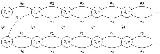
Figure 1.
Generic queueing system.
Let denote the stationary probability that there are n customers in the system and the server is in state ℓ. The balance equations then read
for , while for , we have
By introducing the row vectors , the system of balance equations can be rewritten as follows:
with
for , and with
The system of equations clearly admits a quasi-birth–death (QBD) structure [27], where the system size is the level and the state of the server is the phase of QBD. As we allow for the specification of different rates for different system sizes, the QBD structure is non-homogenous. We discuss numerical solution methods for homogenous and non-homogenous the QBD structures in the next section.
Due to the absence of transitions from the active to the vacation state when there are customers in the system, we can recursively calculate the probabilities and as follows: First, we express and in terms of and :
Plugging these expressions in the balance equations, isolating the terms in and and solving for and yield the following recursion:
for , with
Now, we first assume that the queueing system has a finite capacity N (we then have ). For ease of notation, let and be defined as follows:
The normalisation condition of the Markov chain then reads
Moreover, accounting for the finite capacity, the balance equation for state reads
or
Combining the former expression with the normalisation condition then yields
and
Finally, we find the stationary probabilities by plugging the expressions for , , and in Equation (1). For infinite-capacity generic queueing system with working vacations, we can approximate the infinite-capacity system by a finite-capacity system [28]. The finite capacity needs to be determined by trial and error. A numerical approach is the only viable option if no further assumptions are imposed on the transition rates. However, more explicit results can be obtained for specific rates. We discuss several specific instances below.
2.2. Queue with Working Vacations
We first consider the case where neither the arrival rate nor the service rate depends on the system content, i.e., , and , such that we have an queue with arrival rate and service rates and depending on the state of the server. Moreover, by assuming exponentially distributed vacations with rate , we set for . The value depends on the vacation policy. In a single working vacation, the system remains idle when it finds an empty queue upon returning from vacation (), while in a multiple-vacation system, the server immediately leaves for another vacation ().
This -type (multiple) working vacation queue was first analysed by Servi and Finn [5] by using transform techniques. Liu [8] considers the same model, focussing on stochastic decomposition results. We here explicitly solve the balance equations. To solve the homogeneous second-order linear recursion
we solve the characteristic equation
It is easy to show that the characteristic equation has one root in the interval , while the second root is larger than 1:
As is a probability, we can exclude solutions that involve the second root. Therefore, we find
In view of the expression above, the probabilities satisfy the following second-order non-homogeneous difference equation:
The characteristic equation of the homogenous difference equation has roots 1 and . As is a probability, we can exclude solutions that involve root 1. The solution of the non-homogeneous difference equation is the sum of a particular solution and the solution of the homogeneous difference equation. By proposing a particular equation , we have
Here, the second equality uses the fact that solves characteristic Equation (2). Finally, we have
The remaining unknowns and follow from the balance equations for and the normalisation condition. For the queueing system with multiple working vacations, we find
This solution is in line with the findings of Reference [5]. For the single-vacation system, we have
2.3. M/M/c Queue with Synchronised Working Vacations
For the Markovian multiserver queue, the servers either simultaneously leave for working vacations of identical duration or each server takes a working vacation whenever there is no work when the server becomes available. In the former case, all servers are either active or on vacation, in line with the generic assumptions above. This vacation policy is referred to as synchronised working vacations [20,29]. In the latter case, we need to describe each server’s state individually. Such systems are discussed in the next section.
Assuming that there are c servers, each with service rate , and assuming an arrival rate , the synchronous working vacation system is obtained by assuming
As for the single-server system, we set for . The value depends on the vacation policy. In a single working vacation, the system remains idle when it finds an empty queue upon returning from vacation (), while in a multiple-vacation system, the server immediately leaves for another vacation ().
For we have fixed arrival rate and service rate . Hence, we can again solve the homogeneous second-order linear recursion for first, followed by solving the non-homogenous recursion for . We find that
where and equal
We now need to determine the probabilities and for . To this end, we can either adapt the recursive solution approach of the generic model to account for the expressions for and above, or we can combine these expressions with the balance equations and solve the finite system of equations directly. In either case, we can express the normalisation condition in terms of the unknowns as follows:
With a slight abuse of notation, let , , and be defined as in Section 2.1 but with the current assumptions on , and . These -values can be recursively calculated for and express the unknown probabilities and in terms of and . In view of Equation (4), the balance equation for reads
Noting that the probabilities and can be expressed in terms of and and solving for yield
Finally, the remaining unknown probability can be determined by the normalisation condition
2.4. Further Comments
Most work on -type working vacation queues rely on transform techniques (see, for example, [5,11,12,17]) or on matrix-analytic methods (see, for example, [7,23]). We here opted to solve the recursions for the stationary probabilities directly, to highlight that the vacation probabilities can be determined first (up to a normalising constant). Transform techniques offer a convenient approach to solving the recursions, while the moment-generating property of the transform readily leads to expressions for the moments. However, if the transition rates depend on the system size in a non-trivial way, the transform expressions often cannot be simplified. In this case, the added value of the transform approach is limited. We defer the discussion of the matrix-analytic techniques to the next section.
The approach presented above for the queue with synchronous vacations relies on the recursive calculation of the first probabilities by the generic approach of Section 2.1. As this approach does not assume specific transition rates, the analysis in Section 2.3 can be easily extended to infinite-capacity queues where the transition rates do not depend on the system content beyond a certain level. For the queue, the service rate equals when the system content is at least equal to c, while the arrival and vacation rates do not depend on the system content at all. Not only the service rate can change. For example, the authors in [25] assume repeated vacations until there are at least N customers in the system. In this case, we have for and for . Both service and arrival rates do not depend on the system content.
The generic queueing model with working vacations does not cover all QBD working vacation models with state space . Some authors also allow for vacation interruptions: both the service and the working vacation simultaneously end [7,13,21]. This means that there are transitions from states to states , which are not allowed in the generic model. However, the property that there are no transitions from the active to the vacation state is retained. This is the essential property which allows for the calculation of the probabilities first.
We did not discuss the calculation of the sojourn time distributions in the discussion above. However, most contributions in the literature assume Poisson arrivals with constant arrival rate , while the system dynamics guarantee that customers arrive and depart one by one. These two properties are sufficient to apply a distributional form of Little’s result [30]. Let denote the probability-generating function of the system content:
The Laplace–Stieltjes transform of the sojourn time then equals
Finally, it is worth pointing out that various authors also have investigated the transient characteristics of working vacation queueing systems [19,31,32,33,34,35,36,37,38]. In contrast to the analyses above, a transient analysis investigates how characteristics like the mean queue content vary over time if one starts from a given state or a given distribution over the states.
3. Quasi-Birth–Death Queues
As already mentioned, the Markov chains that represent the working vacation queueing systems in the preceding section exhibit a QBD structure, where the number of phases is limited to two, as the phase represents the server state, which is either available or on vacation. A more versatile model can be obtained by extending the number of phases. More phases allow for the introduction of correlated arrivals (Markov arrival processes) and phase-type distributed service and vacation times [39,40,41,42,43]. Moreover, the state of individual servers can be tracked in multiple-server systems [29,44,45]. We first recall the basic assumptions on generic QBD structures and their numerical (matrix-analytic) solution methods, and then discuss several specific QBD-type working vacation models. Matrix-analytic methods for working vacation queues are also surveyed in [46].
3.1. Balance Equations
We extend the modelling assumptions of the preceding section by (i) extending the 2 server states to K environment states and (ii) allowing for environment transitions when customers enter or leave. The resulting Markov model is then just a generic QBD structure. The environment state represents the phase of the QBD structure, while the system content corresponds to the level. The models do not specifically correspond to queues with working vacations. In principle, we could separate environment and server states and restrict the possible server transitions. This would, however, complicate the notation while having limited benefits for numerical analysis.
Let denote the finite set of environment states, and the number of environment states is denoted by K. When there are n customers in the system, the arrival rate that triggers a transition to environment state ℓ equals in environment state k. Further, let denote the departure rate from state k with a transition to state ℓ when there are n customers in the system, and let denote the rate to transition from environment state k to state without arrivals or departures. Let denote the stationary probability that there are customers in the system and that the environment is in state . The balance equations then read
for , while for , we have
To simplify the notation, we collect the probabilities at level n in the row vector . The balance equations can then be rewritten as follows:
for and
Here, the matrices , and equal
While it is possible to find a closed-form solution of the balance equations for some specific examples, the class of queueing systems that can be analysed by numerically solving the balance equations is considerably wider. We discuss solution methods for both homogenous and non-homogenous QBD structures below.
3.2. Homogenous QBD
We first consider the case where the matrices , and do not depend on level n. Following the notation of Latouche and Ramaswami [27], we set
Assuming that a QBD structure is irreducible, it is ergodic provided that the following drift condition holds:
Here, is the stationary solution of the phase process:
with being a row vector of ones. Some simple calculations then yield the following expression for vector :
Provided that the QBD structure is stationary ergodic, the stationary probabilities conform to
where R is a matrix which conforms to the following quadratic equation:
We can numerically solve this equation by setting and by iteratively calculating
We have for . Moreover, the largest eigenvalue of R is less than one, such that converges. Finally, we find from
and the normalisation condition
Here, I is the identity matrix. The recursive scheme above for solving the QBD structure is but one of the many solution methods for QBD structures. More advanced methods are discussed in [27,47] and the references therein. With a slight modification, the same method also applies if the matrices , and depend on the level for a finite number of levels, e.g., up to level N. We then have , while the vectors to follow from solving the (inhomogeneous) balance equations for the first N levels and the normalisation condition.
3.3. Non-Homogenous QBD
Solving non-homogenous QBD structures is considerably more complex. First, we consider an inhomogeneous QBD structure with a finite number of levels . The consecutive vectors relate as
where the matrix now depends on the level. The level-dependent R-matrices can be recursively calculated as follows:
for . These expressions then allow for the determination of the stationary probabilities up to a normalising constant. Let be the unnormalised vectors which can be recursively calculated as follows:
Finally, the stationary probabilities are found by normalising
The same method can also be applied for non-homogeneous QBD structures with unbounded levels. In this case, one truncates the state space to a sufficiently large level.
3.4. Examples
We now describe several examples in more detail. We start with two homogeneous QBD structures and end with a heterogenous QBD structure. For each example, we discuss the balance equations and give expressions for the block matrix representation of the balance equations.
3.4.1. MAP/M/1 Single-Working Vacation Queue
A Markov arrival process (MAP) is a point process where a Markov process governs the interarrival times between consecutive events. Let us consider a continuous-time Markov process with state space , with transition rate between state k and state without arrivals with rate and with transition rate between state k and state ℓ with arrival with rate . For ease of notation, we set in the remainder.
Let denote the stationary probability that there are n customers in the system while the server is active and the arrival process is in state ℓ. Moreover, is the corresponding probability when the server is on working vacation. The balance equations then read
and
Here, is the indicator function which is 1 if its argument is true and 0 otherwise. Moreover, for all k.
Let denote the state space of the environment. To find the block matrix representation of the QBD structure, let us recall that collects the transition rates with a transition from a lower level, collects the state transitions without level transitions and collects the transition rates with a transition from a higher level. There is a transition from state to state with rate
There is a transition from state to state with rate
Finally, there is a transition form state to state with rate
These transition rates completely specify the matrices , and . Clearly, the QBD under study is homogeneous. Hence, we can solve the set of balance equations by the methods discussed in Section 3.2.
3.4.2. Multiserver Queue with Working Vacations
We already discussed the multiserver queue with synchronised vacations in Section 2.3. With synchronisation, all servers are either on working vacation or not. If there is no synchronisation, one must (at least) track how many servers are on working vacation. We adapt the model from [44] to align with the notation of Section 2.3. The authors implicitly assume that customers move from a server on vacation to an active server if a service on an active server completes and no customers are in the queue. With this assumption, the Markov state of the system is described by the number of customers in the system and the number of active servers. Let us recall that there are c servers and the service rate of a single server is denoted by when the server is active and by when the server is on vacation. The arrival rate is denoted by , and vacations end with rate . Let denote the probability that there are n customers in the system while there are k servers active. We then have the following set of balance equations:
with for and .
To find the block matrix representation of the QBD structure, let us recall that collects the transition rates with a transition from a lower level, collects the state transitions without level transitions and collects the transition rates with a transition from a higher level. From the balance equations, we find the transition rates
which do not depend on the level for . These transition rates completely specify the matrices , and . As the matrices do not depend on the level for , the QBD structure can be solved by the modification for homogeneous QBD structures discussed in Section 3.2.
3.5. Retrial Queue with Vacation Interruptions
As an example of a non-homogenous QBD structure, we briefly discuss the retrial queueing system with vacation interruptions by Li, Zhang and Gao [48]. In retrial queueing systems, customers do not wait at the server but join an orbit and periodically check the server state (see Section 6.1). The retrial rate grows with the number of customers in orbit, leading to non-homogenous QBD structures.
An queue with working vacations and vacation interruptions is characterised as follows: Customers arrive in accordance with a Poisson process with rate . If the server is not occupied, the customer is served immediately, while the customer joins the orbit if this is not the case. Each customer in orbit retries with a rate such that the total retrial rate equals if there are n customers in orbit. The server serves customers at rate if active and if on working vacation. The server leaves for a working vacation if the system is empty (no customer being served and no customers in orbit). The working vacations are exponentially distributed at rate . If the system is empty upon returning from a vacation, the server immediately leaves for another vacation. If the system is non-empty upon completing a service, the working vacation ends, and the server returns to normal.
Let denote the number of customers in orbit, and let denote the server state. The server is either active (a), idle (i) or on working vacation (v). The process then constitutes a QBD structure, with being the level and being the phase. We find the following set of balance equations:
for . Let the vector collect the level n probabilities; we then have
with
and
Clearly, the numerical approach of Section 3.3 applies. In this particular instance, it is, however, also possible to analytically solve the balance equations through transform techniques. We refer to Reference [48] for details.
4. General Service Times
In this section, we discuss queueing systems with non-exponentially distributed service times. To facilitate the analysis it is often convenient to study such queueing systems at embedded time epochs where a countable Markov chain can describe the state of the system. When only the service times are not exponentially distributed, one can study the working vacation system at departure epochs [49]. If the vacations are also not exponentially distributed, one may consider epochs at which either a vacation starts or a service starts during an active period [50]. The analysis of the queue with working vacations below most closely relates to the analysis in [49]. However, we directly introduce the transforms of the queue content at departure epochs and do not describe the corresponding balance equations first.
4.1. Queue
We consider an queueing system with working vacations. The service times of the consecutive customers now have a general distribution, while the interarrival times and the vacation lengths are exponentially distributed. As before, let denote the arrival rate, and let denote the rate of the working vacations. We need to differentiate between service times when the server is active and (longer) service times during working vacations. Moreover, the server can return from a working vacation during a service time. If this is the case, we can either immediately adapt the server speed, or we can only change the server speed upon completion of the service. In the remainder, we consider the following two options:
- We assume that the consecutive service times constitute a sequence of independent and identically distributed random variables, with common distribution function () and corresponding Laplace–Stieltjes transform . During working vacations, the server slows down and takes time units to finish a single unit of service time. Here, is a constant multiplier. Let denote the probability-generating function of the number of arrivals during a service time that starts when the server is active. By conditioning on the length of the service time, we find thatHere, denotes the probability mass function of a Poisson random variable with mean x:When service starts during a working vacation, the server may or may not be active during the service time. We, therefore, consider both the (partial) probability-generating functions and of the number of arrivals during a service time when the server remains on vacation or returns to the active mode, respectively. By conditioning on the length of the service time and the remaining length of the working vacation, we find that
- Alternatively, we assume that the distribution of the service time depends on the server state at the start of the service. Let and denote the Laplace–Stieltjes transforms of the service times when the server is active and on vacation, respectively. With , and defined as above and by conditioning on the end of the working vacation during the service time, we find that
The remainder of the analysis expresses the performance metrics of interest in terms of the probability-generating functions , and and proceeds independently of the specific working vacation policy option that is chosen.
We first investigate the queue content and server state at the departure instants. Let denote the stationary probability to leave n customers behind upon departure, while the server was active just prior to departure. The probability is defined likewise, when the server was on working vacation just prior to departure. It is more convenient to track the server state immediately before departure, while it easily relates to the state after departure: the state is retained if the queue is non-empty, while the server starts a working vacation if the queue is empty.
We here present a probability-generating function approach to simplify the analysis. To this end, let and denote the partial probability-generating functions of the queue content, when the server is active or on working vacation, respectively:
Let denote the queue content at the kth departure epoch, and let denote the number of arrivals during the kth service time. We then have
with as usual. Let denote the server state immediately before this epoch, and let denote the indicator that a working vacation ends during the kth service time. The server state before the st departure then equals
Indeed, the server is only active if it was active and the queue was non-empty or when a vacation ended during the service time. These recursive equations now allow for the expression of the probability-generating functions of the queue content at the st departure epoch in terms of the generating functions at the preceding departure epoch. By using standard transform manipulations and noting that these generating functions are equal for the stationary queue process, we find that
Solving for and further yields
where only the probabilities and are unknown. To determine the remaining unknowns, let denote the unique solution of in the interval . As probability-generating functions are analytic in the open unit disk, the zero of the denominator also needs to be a zero for the numerator, which yields . The remaining unknown probability then follows from the normalisation condition:
By using L’Hôpital’s rule to evaluate in , we find that
Let denote the probability-generating function of the queue content (without conditioning on the server state). By combining the former expressions, we find
Following the arguments for the Markovian queues with Poisson arrivals above, the probability-generating functions of the queue content at departure epochs, arrival epoch and random epochs coincide. Hence, is also the probability-generating function of the queue content at random epochs. Moreover, by the distributional form of Little’s result, the Laplace–Stieltjes transform of the sojourn time is given by Equation (7), with as defined in Equation (11).
4.2. Further Comments
Most papers that consider working vacation queues with generally distributed service times assume that the vacations are exponentially distributed. Such an assumption greatly simplifies the analysis. Wu and Takagi [50], however, show that results can still be obtained if one assumes vacation distributions that have a rational Laplace–Stieltjes transform. Methodologically, most analyses rely on transform techniques and first focus on the queue process at departure times. If customers enter and leave one at a time, the queue size distributions at departure and arrival times are equal. Moreover, for Poisson arrivals, the queue size distribution at arrival times and at random points in times are also equal by the PASTA property (Poisson Arrivals See Time Averages).
Various authors propose extensions of the basic working vacation queue with generally distributed service times. For example, Murugan and Santhi [51] include random system breakdowns which require repair before the system can resume serving customers. Like breakdowns, in a system with disasters, the system stops working when a disaster occurs. Such disaster, however, not only interrupts service but also clears the queue [52]. Afanasyev [53] introduces close-down times. These close-down periods precede vacation periods, and the following vacation period is cancelled if there are arrivals during the close-down time. Systems with vacation interruptions have gained particular attention [54,55,56,57]. A vacation interruption breaks off the vacation at the end of a service time if there are waiting customers.
All vacation systems discussed so far are so-called exhaustive vacation systems. In an exhaustive vacation system, a vacation only starts if there are no customers in the system. In contrast, in a gated vacation system, vacations start if there are no customers in the system that arrived prior to the start of the preceding vacation. Saffer and Telek [58] introduce gated working vacations in a similar manner. During an active period, only customers that were present at the start of the active period are served. A new working vacation starts once all these customers have received service. During the working vacation, the server starts processing the customers that arrived during the active period, as well as any arrivals during the vacation period. Once the server returns from the working vacation, a new active–vacation cycle starts.
The inclusion of so-called batch arrivals—customers arrive in groups of random size, rather than one at a time—often does not complicate the transform-based analysis in the above-mentioned working vacation queues and related queues. Indeed, the probability-generating function of the sum of a random number of independent and identically distributed discrete random variables equals , where denotes the probability-generating function of the number of terms in the sum and denotes the probability-generating function of a term. By applying this property, one e.g., immediately finds that the probability-generating function of the number of arrivals during an active period equals (see Equation (8)), with the probability-generating function of the batch size distribution. This extension applies to the complete analysis of the queue content on departure times. The analysis at random times requires an additional renewal-type argument to relate the queue distribution as seen by arriving batches to the queue distribution as seen by arriving customers. See, e.g., [59,60,61], for working vacation queueing systems with batch arrivals.
If one focuses on the embedded Markov process in an queue (with working vacations) at departure times, the queue size drops by at most one between departures, while the queue can grow to any value between departures. Markovian systems that possess a similar property are referred to as -type queueing systems and relate both to the queue and to the quasi-birth–death systems of the preceding section. To be precise, an -type queueing system is a Markovian queueing system where the state is described by a level and a phase, with the number of possible phases being finite. Upward transitions between any levels are allowed, while downward transitions are only allowed between adjacent levels. Examples of Markovian -type queueing systems with working vacations include [62,63,64,65], where upward transitions stem from batch arrivals.
5. General Interarrival Times
Various authors consider working vacation systems where the interarrival times constitute a sequence of independent and identically distributed random variables. Baba considers the multiple working vacation system with exponentially distributed service time and vacation times [66]. Banik, Gupta and Pathak [67] consider the same system but assume that the queue has finite capacity. We first present an alternative analysis of Baba’s model and then briefly discuss a number of related models.
5.1. G/M/1 Queue
We retain the assumptions and notation of the multiple-vacation model of Section 2.2, apart from the assumptions on the arrival process. We now assume that the consecutive interarrival times constitute a sequence of independent and identically distributed random variables, with common cumulative distribution function and corresponding Laplace–Stieltjes transform . Let denote the arrival rate. By the moment-generating property of Laplace–Stieltjes transforms, we have
We further retain the notation and for the service rates when the server is active and on working vacation, respectively. Moreover, a working vacation ends at a rate .
We first consider the system at arrival times. Clearly, the server and queueing state at consecutive arrival times constitute a discrete-time Markov chain, as the vacation and service times are exponentially distributed. Let and denote the stationary probability that the arrival finds n customers, and an active server and a server on vacation, respectively.
As we describe the system at arrival instants, we first calculate the probability mass functions of the number of (potential) departures between arrivals and corresponding (partial) probability generation functions. The definitions below count the number of customers that would depart if there were an infinite supply of customers and do not account (yet) for the system becoming empty between arrivals. More precisely, let denote the probability that there are k departures during an interarrival time when the server is active at the start, and let denote the corresponding probability generation function:
Analogously, let denote the probability that there are k departures during an interarrival time when the server remains on vacation for the entire duration, and let denote the corresponding probability generation function:
Finally, let denote the probability that there are k departures during an interarrival time when the server is on vacation at the start and becomes active before the next arrival:
The expression above conditions on the time the server becomes active. The corresponding probability-generating function equals
We now easily express the balance equations in terms of these probabilities. We first consider the balance equations when the queue is not empty. The server is active if it was already active at the previous arrival or becomes active during the interarrival time. The server is on working vacation only if it was already on working vacation before. Hence, we find
for When the server is empty, we account for the change to a working vacation when the queue becomes empty.
To solve the balance equations, we first solve the system for the working vacation probabilities, similar to the approach for the working vacation queue in Section 2.2. The balance equations for are equivalent to the balance equations of the queue. Hence, we have a geometric solution, and we set
which yields
or
One easily shows that for , there exists a unique real solution in the interval . Indeed, the function is negative in , positive in and convex in the interval .
By plugging in solution (12) into the balance equation for , we have the following non-homogenous difference equation for the probabilities when the server is active:
To solve this difference equation, we first solve the corresponding homogenous difference equation. The characteristic equation of this homogenous difference equation reads
This characteristic equation has a unique solution for , and we find that the solution of the homogenous equation is proportional to . The solution of the non-homogenous equation is the sum of the solution of the homogenous equation and a particular equation. Let us assume that the particular solution has the form . By substituting the proposed particular solution in Equation (13) and by solving for , we find
The corresponding solution of the non-homogenous difference equation then equals
where we used the equality to determine the factor of the homogenous term.
Finally, the remaining unknown probability follows from the normalisation condition
Solving for yields
Summarising, we find the following solution for the balance equations:
As PASTA (Poisson Arrivals See Time Averages) does not apply in the present setting, some additional work is required to find the distribution of the number of customers in the queue at random points in time. By the renewal theory, the time that elapsed since the last arrival has the following density function and corresponding Laplace–Stieltjes transform :
We can now enumerate all possible scenarios that lead to a certain state at a random point in time. When the queue is active, either it was already active when there was a previous arrival, or it became active during the interarrival time. Conditioning on the number of customers found in the system by the last arrival and on the time the server returns back from a working vacation yields
By interchanging the order of the sum and integrals, the former expression simplifies to
Plugging in the expression for the transform further yields
When the server is on working vacation and the queue is not empty at a random observation epoch, the preceding arrival finds the server on vacation, and the vacation does not end prior to the observation epoch. Conditioning on the number of customers in the system at the preceding arrival instant then yields
for , or equivalently,
Plugging in the expression for the transform further yields
Finally, we can use the normalisation condition to find the remaining probability :
5.2. Further Comments
We conclude this section on working vacations with generally distributed interarrival times with a discussion of various extensions of the basic queueing model. The basic model above assumes that the server takes multiple consecutive vacations if the server is empty upon returning from a vacation. Various authors also consider the working vacation where the server only takes a single vacation [68,69]. Other authors also focus on the finite working vacation queue [67,70,71,72], where customers cannot enter upon arrival if the queue is full. As for the queue, working vacation systems with vacation interruption have also been investigated [73,74]. Let us recall that the term vacation interruption refers to the possibility to end the vacation if there are waiting customers at the end of a service time. There is a considerable interest in batch service queues with working vacations and generally distributed interarrival times [75,76,77]. In a batch service queue, customers are served collectively, rather than individually. Once there are enough customers waiting, a batch service starts, and all customers in the batch leave the queue at the end of the batch service. Finally, Ouazine and Abbas [78] investigate a finite-capacity multiserver queue with synchronised working vacations. Let us recall that in such a multiserver vacation system, all servers simultaneously leave for a vacation if there are no more customers in the system.
6. Other Queueing Systems with Working Vacations
While the models in the preceding sections present an overview of the various modelling assumptions and analysis techniques, there are multiple areas of research on working vacation models that have not been discussed. In this section, we briefly discuss some of these diverse areas that have attracted considerable interest.
6.1. Retrial Queues with Working Vacations
In a retrial queueing system, customers do not wait to receive service at the server but come back at a later time, until they find the server available. The set of customers that will return at a later time is referred to as the orbit, and customers typically return after spending an exponentially distributed time in orbit. Even when all service and interarrival times are exponentially distributed, the server can be in one out of four states: busy or idle and active or on a working vacation. Moreover, the overall retrial rate depends on the number of customers in orbit (the total rate being the sum of the retrial rates of the customers in orbit), unless a so-called single-retrial policy is adopted (there is a fixed retrial rate independent of the number of customers in orbit). Hence, retrial queues are in general more difficult to analyse than the corresponding queueing system where the customers wait at the queue.
In the Markovian setting, many retrial queueing models are specific instances of quasi-birth–death processes, with the phase being the state of the server and the level being the number of customers in orbit. Most authors adopt a single-retrial policy, which leads to a homogenous QBD structure [79,80,81,82,83], while the retrial rates depend on the level if all customers can retry [48]. Retrial queues with generally distributed service times have also been investigated [84,85,86]. These papers rely on the supplementary variable method and again adopt a single-retrial policy. Other extensions of the basic Markovian models include multiserver models [87], priority models [88] and batch arrival models [89,90].
6.2. Working Server Breakdowns
Various terms have been used in the literature to indicate periods where the server is absent or working at a reduced rate. We have so far reserved the term “queueing system with working vacations” exclusively for queues where these periods start when the queue becomes empty. Systems where the periods with a reduced service rate start independently of the queue size are most commonly referred to as queueing systems with working breakdowns. In the literature on queues with vacations, the term “(service) interruptions” is also used to refer to such breakdowns. However, for working vacation systems, interruptions more commonly refer to vacation interruptions, events that effectively end the working vacation instead of starting one [91,92].
Working breakdowns closely relate to queues where the service rates are modulated by an external Markov process. For working breakdowns, no breakdowns start when the server is idle, while modulation allows one to move to the low service rate state when the queue is empty. Many authors consider Markovian breakdown queues: The queue with working breakdowns is investigated in [93]. Some notable extensions of this basic model include the presence of batch arrivals [94], customer balking and reneging [95]. Moreover, queueing systems can both be subject to working vacations and working breakdowns [96,97]. Finally, in [98], a bulk service queue is considered with generally distributed (bulk) service times and breakdowns. The authors assume that breakdowns occur when service finishes, thereby preventing the breakdown from interrupting the service.
6.3. Discrete-Time Working Vacation Queues
In discrete-time queueing theory, time is a discrete quantity. Time is divided into fixed-length intervals, referred to as slots. All arrivals to and departures from the queues are synchronised with respect to slot boundaries. The discrete-time assumption is sometimes motivated by a clock time in computer or communication systems, though for sufficiently small slots, the difference in performance between a continuous-time queueing system and a corresponding discrete-time queueing system is limited. The role of exponentially distributed random variables is played by the geometric distribution in discrete time. From a mathematical vantage point, there are some key differences. First, there may be multiple events (arrivals, end of service, vacation times, etc.) at the same slot boundary. This often implies that the number of transitions from a single state is larger, which might complicate the analysis. Secondly, single-slot deterministic service times fit the Markovian setting, as a single-slot service time is a geometrically distributed service time with success probability 0. Finally, as time-related quantities are discrete, it is often possible to describe state transitions between slots, even for non-geometric service and arrival distributions, by the inclusion of supplementary variables in the state description.
The literature on discrete-time queues with working vacations starts from similar assumptions and relies on similar analysis techniques to their continuous-time counterparts. We can again discern Markovian queues [99], G/M/1 (or G/Geo/1) queues [100,101,102] and M/G/1 (or Geo/G/1) queues [60,103,104,105]. Both transform-based approaches [100,101,102,106,107] and matrix-analytic techniques [99,108,109] have been explored.
6.4. Fluid Queues
When the interarrival and service times are shorter than other processes, like vacation times, interruption times or repair times, it is reasonable to assume that arrivals and departures can be modelled as fluids entering and leaving some storage or queue. The fluid models with working vacation queues can be divided into two distinct classes. First, some authors have recently modelled the arrivals and departures in the working vacation queue as fluids [110,111]. As the net fluid input in a fluid queue is simply the difference between the input and output (fluid) rate, the server leaving for a working vacation corresponds to a different net input rate.
Earlier work on fluid working vacation queues, however, follows a different approach. The Markovian working vacation queue is used to modulate (or drive) the net input rates in another queue [112,113,114,115,116,117,118]. More precisely, depending on the state of the working vacation queue, the fluid queue changes following a different net input rate, though the number of possible rates is a finite set. Typically, there are different rates when the queue is empty or not and when the queue is on vacation or not.
7. Queueing Games
Queueing games combine elements of queueing theory and game theory to analyse strategic customer choices. In queueing games, players make decisions about when or how to join the queue, with the goal of minimising cost. The cost here typically refers to (waiting) time, money, or both. A key assumption in any queueing game is what information is available to the customers. For games that study customer balking strategies in working vacation queues, the information can include the queue length and the server state when the customers arrive at the system. Customers may also be unaware of any state information (unobservable queueing games). Queueing games with working vacations have attracted considerable interest. Most authors consider continuous-time Markovian queueing games [119,120,121,122,123,124,125,126,127,128,129,130,131,132,133,134,135,136,137,138,139,140,141,142,143]. Some authors also consider discrete-time queueing games [144,145], non-Markovian games [146,147,148] and games based on fluid models [110,111]. We discuss in some detail how observability leads to different models for the working vacation queue below, before surveying some of the literature.
7.1. The Game with Multiple Working Vacations
Let the reward R be expressed in terms of sojourn times. R corresponds to the sojourn times customers are willing to undergo. Hence, if the expected waiting time of a customer exceeds this cost, the customer does not join the queueing system. This expected waiting time accounts for all the information on the queueing process that is available to the customer.
In the unobservable queueing game, customers are only aware of the parameters of the system and not of the state of the queueing system upon arrival. Hence, customers join the queue upon arrival with probability p, such that the expected sojourn time does not exceed the cost R. From the stationary distribution in (3) and Little’s result, one easily finds that the expected sojourn time when customers enter with probability p equals
with
One can show that is an increasing function in p. This is not unexpected, as more customer arrivals imply longer expected waiting times. If , all customers balk, as no customer has an incentive to join. If , all customers join. For , there exists a unique mixed strategy which solves . Uniqueness follows from the fact that is a continuous and strictly increasing function.
In the fully observable scenario, customers are aware of the state of the system (system content and server state). Hence, customers join if the expected sojourn time conditional on the observed state is less than R.
where we used to solve the recursion. Both and are unbounded and increasing in n, with . Hence, there exist thresholds such that customers join when the system content does not exceed the threshold and the server is on vacation and active, respectively.
Finally, customers may also be only aware of the system content. The expected sojourn time, conditional on the system content, equals
where and are the stationary system content probabilities, assuming that the customers balk if the system content is equal or exceeds a threshold T. The solution of this partially observable queueing game is then found by determining T such that for and .
7.2. Customer Heterogeneity
The game in the preceding subsection assumes that all customers perceive waiting times alike. Some customers may, however, value the service more than others and therefore be willing to wait longer. Customer heterogeneity is most easily accounted for by introducing random non-negative rewards R. That is, let
denote the probability that a customer receives a reward of at least t time units. Hence, when customers expect a waiting time , a fraction will join the queue, while the others will balk. For mathematical convenience, we assume that is continuous and strictly decreasing. These assumptions imply that the function is well defined for all . Moreover, is a strictly decreasing function, with and .
We first consider the unobservable game with heterogenous customers. In this case, the equilibrium p solves , with as given in Equation (16). As decreases from ∞ to 0 and increases when p increases from 0 to 1, there exists a unique solution of the unobservable game. For the fully observable game, the waiting time expressions in (17) for the different states still hold. Hence, the fractions of customers and that join in states and equal
The fully observable game leads to a Markov chain with state-dependent arrival rates and , as discussed in Section 2.1.
7.3. Further Remarks
The analyses above only sketch how game-theoretic arguments can be combined with queueing analyses for the simplest instance of joining strategies for a working vacation queue. These arguments have been applied on more intricate working vacation queues in the literature. Some more intricate working vacation models that have attracted considerable attention include retrial queueing models [132,135,136,140,148], queues with working vacation interruptions [123,124,129,130,137,139,147] and queues with working breakdowns [119,128,135,136,145,148].
The game setting assumes that customers optimise their own utility: under equilibrium, no customer has an incentive to change their joining strategy. This, however, does not mean that customers receive the best possible performance. The performance gain that can be achieved by imposing a socially optimal strategy is often referred to as the price of anarchy [111]. If all customers follow the socially optimal strategy, individual customers may benefit from changing strategy (but are prevented from doing so). Some authors also investigate how specific pricing can be used to incentivise customers to follow the socially optimal strategy [141,148]. Note that some authors refer to socially optimal strategies as cooperative strategies [135,140,148], although the arguments rely on optimisation techniques rather than on the arguments of cooperative game theory.
The game-theoretic arguments can further be combined with revenue management [133,141]. Revenue management refers to how the service provider can optimise their utility by setting the prices and possibly other parameters of the queueing system. From the service provider’s perspective, revenue management seeks a trade-off between the revenue per customer and the fraction of customers that join the queue.
8. Applications
We now discuss some specific applications of queueing models with working vacations. Applications stem both from particular performance problems for computer and telecommunication systems or from manufacturing and service systems.
8.1. Ethernet Passive Optical Networks
Ethernet Passive Optical Networks (EPONs) use a single optical fibre to deliver broadband internet by splitting signals to multiple endpoints through passive optical splitters. Downstream traffic towards the endpoints is broadcasted and filtered by the optical network units at the endpoints. To avoid simultaneous upstream traffic transmissions, the bandwidth is split by a multipoint control protocol which makes the time and/or wavelength allocations for the different end users. Various authors have addressed EPON performance through working vacation models.
In an EPON with wavelength division multiplexing, every endpoint is assigned a permanent wavelength. Additional wavelengths can be assigned to the endpoints to increase the available bandwidth. These wavelengths are then released by the endpoints when their packet queues are empty. Various authors [149,150,151] note the correspondence with working vacation queues. The assignment of additional wavelengths corresponds to increasing the service speed (active state), while the service speed is reduced when the queue becomes empty (working vacation state). The presence of dedicated wavelengths naturally leads to working vacation queues as service continues at a lower rate when no other wavelength or time slots are assigned to the endpoint. If the endpoints have no dedicated channel, the performance is captured by classic vacation or polling models.
8.2. Power-Saving Protocols
Energy consumption is a key concern for many network components, ranging from wireless devices to servers in data centres or the overall energy consumption in peer-to-peer networks. Energy reductions are basically obtained by turning off servers when there is no need for services. As servers are turned off when there is no work, queueing models with vacations are well suited to investigate how power saving affects services, as well as energy consumption. In many practical scenarios, service is not completely turned off but offered at a lower rate when there is no work. This service speed reduction then corresponds to a working vacation [152].
8.2.1. WirelessNetworks
Motivated by energy consumption in wireless communication networks, Yu et al. [153] and Ma et al. [154] consider Markovian working vacation systems with two servers. Both servers simultaneously enter a working vacation if there are no outstanding packets. Packets during the working vacation are processed by the servers at a reduced rate, and the servers only return from sleep mode if there are at least N packets waiting. The working vacation here corresponds to a transmission speed reduction if there are no packets waiting. Specifically focussing on sleep mode in WiMAX, Shapique et al. [155] consider a working vacation model where the system first takes an ordinary vacation when the system becomes empty, followed by working vacations if needed. The authors motivate this vacation policy by the power-saving classes introduced in IEEE 802.16e.
8.2.2. Data Centres
Power management in cloud computing is essential to realising energy efficiency, thereby reducing operational costs and the environmental impact of large-scale data centres. Idle-resource management moves servers not in use into low-power modes or shuts servers down when demand drops. In queueing terms, the low-power mode corresponds to a working vacation. In [156], Markovian single- and multiple-working vacation models are used to study the energy-performance trade-off of a single physical server. Later, clusters with two servers are investigated in [15,157]. The authors assume synchronised working vacations when the servers move into a power-saving mode (e.g., using dynamic voltage and frequency scaling [15]). Focussing on server virtualisation, Sahoo and Goswami [158] propose a finite Markovian working vacation model for a virtual machine (VM) operating in two modes: active (high computational power during heavy loads) and passive (low power during lighter loads). The VM switches between modes to maintain system performance, reduce energy consumption and meet Service Level Agreements (SLAs) under fluctuating workloads. The findings of Sahoo and Goswami are later extended by Qin et al. [159], who investigate the join state of multiple VMs, and by Guo et al. [160], who combine working vacations with priority scheduling.
8.2.3. Peer-to-Peer Networking
Peer-to-peer (P2P) networking is a network technology which enables peers to exchange resources on equal terms without intermediaries. The peers act both as servers and clients: each peer provides services and sends service requests. A typical P2P network consists of many nodes, which makes the reduction in total energy consumption a pressing concern. One strategy to decrease energy consumption consists of allowing the serving node to cycle between normal mode and sleep mode, with the sleep mode corresponding to the working vacation. In queueing terms, the requesting peers act as customers, whereas the service peers correspond to the servers. As all servers move to sleep mode when there are no outstanding requests, working vacation models with synchronous vacations are proposed to evaluate the performance of peer-to-peer networks [161,162,163].
8.3. Manufacturing and Service Systems
Yang and Tsao [164] consider a repairable system consisting of M primary components and S spare components. There is a single repairperson who leaves for a vacation when all components in the system function properly. During a vacation period, the repairperson lowers the repair rate rather than halting repairs altogether. With exponential failure, repair and vacation times, one easily finds that the system can be modelled by a finite-working vacation queueing system. Gao et al. [165] consider a similar model, with three distinct additional features: the repairperson waits for some time before taking a vacation (a delayed vacation policy), standby components may fail and are repaired first when a component fails, and all components may fail simultaneously. Again assuming exponential failure, repair and vacation times as in Yang and Tsao [164], Yang and Wu [166] study a system where the repairperson randomly leaves for working vacations. This results in a model with working breakdowns during which the repairperson works at a reduced rate.
Ambika et al. [167] consider a working vacation queue in the context of a production system. When there are no pending orders, the manufacturing system undergoes maintenance, which leads to lower service rates. The authors allow for so-called working vacation interruptions at service completion times. When service is completed during a working vacation, the working vacation ends with a fixed probability.
Some authors also include elements from retrial queues with servers that leave for working vacations. The fault-tolerant machining system of [168] accounts for orbits where failed units can wait when the repairperson is occupied. Harini and Indhira [169] propose a batch service working vacation model for a batch production system. The server takes working vacations when there are no products in the system.
While there are many applications of working vacations in manufacturing systems, there are almost no applications for service systems. A notable exception is [170], in which Janani and Vijayashree propose a working vacation model for an intensive care unit. The doctor represents the server who is busy (active state), checking discharged patients through sensor monitoring (working vacation state) or away to follow up on an emergency request (server interruption).
9. Conclusions
This paper has provided a comprehensive overview of queueing systems with working vacations, highlighting their theoretical underpinnings and practical relevance. By extending the traditional notion of server vacations, the working vacation framework captures a richer served dynamic where the server continues to operate at a reduced capacity. Our review emphasises the structural properties of the underlying Markov processes and the diverse analytical techniques employed to evaluate system performance. Additionally, we explore the strategic behaviour of users in queueing games involving working vacations and discuss various real-world applications where such models prove valuable.
We conclude with some potential future research directions. First, for Markovian working vacation queues, the probabilities of the working vacation states can be studied independently of the active states. It would be interesting to investigate if this type of decomposition also applies to other Markovian queueing systems, especially for systems where multiple subsets of states can be studied separately. Secondly, ordinary vacation queues relate to polling systems, not only in the sense that a vacation represents the time the server is not attending a particular queue, but also due to the presence of vacations when the server in a polling system changes from one queue to another. In this vein, polling systems represent a multidimensional extension of vacation queues. It is not clear to what extent multidimensional extensions of working vacation queues are amenable for exact or approximate performance analysis. Finally, although the working vacation concept is a rather natural abstraction, more real-world applications of working vacation queues are needed.
Funding
This research received no external funding.
Data Availability Statement
The original contributions presented in this study are included in the article.
Conflicts of Interest
The author declares no conflicts of interest.
References
- Takagi, H. Queueing Analysis: Vacation and Priority Systems; North-Holland: Amsterdam, The Netherlands, 1991; Volume 1. [Google Scholar]
- Tian, N. Vacation Queueing Models: Theory and Applications; Springer: Cham, Switzerland, 2006. [Google Scholar]
- Doshi, B. Queueing Systems with vacations: A survey. Queueing Syst. 1986, 1, 29–66. [Google Scholar] [CrossRef]
- Tian, N.; Xu, X.; Ma, Z.; Jin, S.; Sun, W. A Survey for stochastic decomposition in vacation queues. In Stochastic Models in Reliability, Network Security and System Safety: Essays Dedicated to Professor Jinhua Cao on the Occasion of His 80th Birthday; Springer: Singapore, 2019; pp. 134–158. [Google Scholar] [CrossRef]
- Servi, L.D.; Finn, S.G. M/M/1 queues with working vacations (M/M/1/WV). Perform. Eval. 2002, 50, 41–52. [Google Scholar] [CrossRef]
- Chandrasekaran, V.M.; Indhira, K.; Saravanarajan, M.C.; Rajadurai, P. A survey on working vacation queueing models. Int. J. Pure Appl. Math. 2016, 106, 33–41. [Google Scholar]
- Li, J.; Tian, N. The M/M/1 queue with working vacations and vacation interruptions. J. Syst. Sci. Syst. Eng. 2007, 16, 121–127. [Google Scholar] [CrossRef]
- Liu, W.; Xu, X.; Tian, N. Stochastic decompositions in the M/M/1 queue with working vacations. Oper. Res. Lett. 2007, 35, 595–600. [Google Scholar] [CrossRef]
- Hui, X.; Chen, H.; Tian, N.; Donghua, L. Study on N-Policy Working Vacation Polling System for WDM. In Proceedings of the International Conference on Communication Software and Networks, Chengdu, China, 27–28 February 2009; pp. 508–511. [Google Scholar] [CrossRef]
- Wang, K.H.; Chen, W.L.; Yang, D.Y. Optimal management of the machine repair problem with working vacation: Newton’s method. J. Comput. Appl. Math. 2009, 233, 449–458. [Google Scholar] [CrossRef]
- Yue, D.; Yue, W.; Xu, G. Analysis of customers’ impatience in an M/M/1 queue with working vacations. J. Ind. Manag. Optim. 2012, 8, 895–908. [Google Scholar] [CrossRef]
- Selvaraju, N.; Goswami, C. Impatient customers in an M/M/1 queue with single and multiple working vacations. Comput. Ind. Eng. 2013, 65, 207–215. [Google Scholar] [CrossRef]
- Laxmi, P.V.; Jyothsna, K. Impatient customer queue with Bernoulli schedule vacation interruption. Comput. Oper. Res. 2015, 56, 1–7. [Google Scholar] [CrossRef]
- Li, J.; Cheng, B. Threshold-policy analysis of an M/M/1 queue with working vacations. J. Appl. Math. Comput. 2016, 50, 117–138. [Google Scholar] [CrossRef]
- Wang, J.; Gao, S.; Do, T.V. Performance analysis of a two-node computing cluster. Comput. Ind. Eng. 2016, 93, 227–235. [Google Scholar] [CrossRef]
- Bouchentouf, A.A.; Yahiaoui, L. On feedback queueing system with reneging and retention of reneged customers, multiple working vacations and Bernoulli schedule vacation interruption. Arab. J. Math. 2017, 6, 1–11. [Google Scholar] [CrossRef]
- Majid, S.; Manoharan, P. Analysis of a M/M/c queue with single and multiple synchronous working vacations. Appl. Appl. Math. Int. J. 2017, 12, 671–694. [Google Scholar]
- Manoharan, P.; Majid, S. Stationary analysis of a multiserver queue with multiple working vacation and impatient customers. Appl. Appl. Math. Int. J. 2017, 12, 658–670. [Google Scholar]
- Sudhesh, R.; Azhagappan, A.; Dharmaraja, S. Transient analysis of M/M/1 queue with working vacation, heterogeneous service and customers’ impatience. RAIRO Oper. Res. 2017, 51, 591–606. [Google Scholar] [CrossRef]
- Majid, S.; Manoharan, P. Impatient customers in an M/M/c queue with single and multiple synchronous working vacations. Pak. J. Stat. Oper. Res. 2018, 14, 571–594. [Google Scholar]
- Majid, S.; Manoharan, P. Analysis of an M/M/1 queue with working vacation and vacation interruption. Appl. Appl. Math. Int. J. 2019, 14, 19–33. [Google Scholar]
- Sun, W.; Li, S.; Wang, Y.; Tian, N. Comparisons of exhaustive and nonexhaustive M/M/1/N queues with working vacation and threshold policy. J. Syst. Sci. Syst. Eng. 2019, 28, 154–167. [Google Scholar] [CrossRef]
- Shekhar, C.; Varshney, S.; Kumar, A. Optimal control of a service system with emergency vacation using bat algorithm. J. Comput. Appl. Math. 2020, 364, 112332. [Google Scholar] [CrossRef]
- Majid, S. Analysis of customer’s impatience in queues with Bernoulli schedule server working vacations and vacation interruption. Afr. Mat. 2022, 33, 1. [Google Scholar] [CrossRef]
- Lv, S.; Wen, J.; Yang, M. The M/M/1 working vacation queueing system with N-policy and different arrival rates. Eng. Lett. 2023, 31, 1–7. [Google Scholar]
- Jyothsna, K.; Kumar, P.V.; Laxmi, P.V. Bat algorithm for optimizing a working vacation queue with impatient clients and secondary service. OPSEARCH 2024, 62, 777–796. [Google Scholar] [CrossRef]
- Latouche, G. Introduction to Matrix Analytic Methods in Stochastic Modeling; Society for Industrial and Applied Mathematics: Philadelphia, PA, USA, 1999. [Google Scholar]
- Wolf, D. Approximation of the invariant probability measure of an infinite stochastic matrix. Adv. Appl. Probab. 1980, 12, 710–726. [Google Scholar] [CrossRef]
- Do, T.V. Comments on “multi-server system with single working vacation”. Appl. Math. Model. 2009, 33, 4435–4437. [Google Scholar] [CrossRef]
- Bertsimas, D.; Nakazato, D. The distributional Little’s law and its applications. Oper. Res. 1995, 43, 298–310. [Google Scholar] [CrossRef]
- Indra; Ruchi. Transient analysis of two-dimensional state Markovian queueing model with working vacation and breakdown. Int. J. Agric. Stat. Sci. 2010, 6, 571–584. [Google Scholar]
- Sudhesh, R.; Raj, L.F. Computational Analysis of Stationary and Transient Distribution of Single Server Queue with Working Vacation. In Proceedings of the 4th ObCom International Conference on Recent Trends in Computing, Communication and Information Technology, Vellore, India, 9–11 December 2011; Volume 269, pp. 480–489. [Google Scholar]
- Yang, D.; Wu, Y. Analysis of a finite-capacity system with working breakdowns and retention of impatient customers. J. Manuf. Syst. 2017, 44, 207–216. [Google Scholar] [CrossRef]
- Ye, Q.; Liu, L. Analysis of MAP/M/1 queue with working breakdowns. Commun. Stat. Theory Methods 2018, 47, 3073–3084. [Google Scholar] [CrossRef]
- Azhagappan, A.; Deepa, T. Variant impatient behavior of a Markovian queue with balking reserved idle time and working vacation. RAIRO Oper. Res. 2020, 54, 783–793. [Google Scholar] [CrossRef]
- Shekhar, C.; Kumar, N.; Gupta, A.; Kumar, A.; Varshney, S. Warm-spare provisioning computing network with switching failure, common cause failure, vacation interruption, and synchronized reneging. Reliab. Eng. Syst. Saf. 2020, 199, 106910. [Google Scholar] [CrossRef]
- Azhagappan, A.; Deepa, T. Transient behavior of a single-server Markovian queue with balking and working vacation interruptions. J. Oper. Res. Soc. China 2021, 9, 321–341. [Google Scholar] [CrossRef]
- Ayyappan, G.; Archana, G. Analysis of MAP/PH1, PH2/2 queueing model with working breakdown, repairs, optional service and balking. Appl. Appl. Math. Int. J. 2023, 18, 1. [Google Scholar]
- Baba, Y. The M/PH/1 queue with working vacations and vacation interruption. J. Syst. Sci. Syst. Eng. 2010, 19, 496–503. [Google Scholar] [CrossRef]
- Sreenivasan, C.; Chakravarthy, S.R.; Krishnamoorthy, A. MAP/PH/1 queue with working vacations, vacation interruptions and N policy. Appl. Math. Model. 2013, 37, 3879–3893. [Google Scholar] [CrossRef]
- Choudhary, A.; Chakravarthy, S.R.; Sharma, D.C. Analysis of MAP/PH/1 queueing system with degrading service rate and phase type vacation. Mathematics 2021, 9, 2387. [Google Scholar] [CrossRef]
- Arulmozhi, N. Analysis of MAP/PH/1 queueing model subject to two-stage vacation policy with imperfect service, setup time, breakdown, delay time, phase type repair and reneging customer. Appl. Appl. Math. Int. J. 2023, 18, 3. [Google Scholar]
- Thakur, S.; Jain, A.; Ahuja, A. Analysis of MAP/PH/1 model with working vacation, working breakdown and two-phase repair. Arab. J. Sci. Eng. 2024, 49, 7431–7451. [Google Scholar] [CrossRef]
- Lin, C.H.; Ke, J.C. Multi-server system with single working vacation. Appl. Math. Model. 2009, 33, 2967–2977. [Google Scholar] [CrossRef]
- Wu, C.H.; Wang, K.H.; Ke, J.C.; Ke, J.B. A heuristic algorithm for the optimization of M/M/s queue with multiple working vacations. J. Ind. Manag. Optim. 2012, 8, 1–17. [Google Scholar] [CrossRef]
- Tian, N.; Li, J.; Zhang, Z. Matrix analytic method and working vacation queues: A survey. Int. J. Inf. Manag. Sci. 2009, 20, 603–633. [Google Scholar]
- Bini, D.A.; Latouche, G.; Meini, B. Numerical Methods for Structured Markov Chains; Oxford University Press: Oxford, UK, 2005. [Google Scholar]
- Li, T.; Zhang, L.; Gao, S. Performance of an M/M/1 retrial queue with working vacation interruption and classical retrial policy. Adv. Oper. Res. 2016, 2016, 4538031. [Google Scholar] [CrossRef]
- Li, J.; Tian, N.; Zhang, Z.G.; Luh, H.P. Analysis of the M/G/1 queue with exponentially working vacations-a matrix analytic approach. Queueing Syst. 2009, 61, 139–166. [Google Scholar] [CrossRef]
- Wu, D.A.; Takagi, H. M/G/1 queue with multiple working vacations. Perform. Eval. 2006, 63, 654–681. [Google Scholar] [CrossRef]
- Murugan, S.P.B.; Santhi, K. An M/G/1 queue with server breakdown and multiple working vacation. Appl. Appl. Math. Int. J. 2015, 10, 678–693. [Google Scholar]
- Kleiner, I.; Frostig, E.; Perry, D. Busy periods for queues alternating between two modes. Methodol. Comput. Appl. Probab. 2023, 25, 60. [Google Scholar] [CrossRef]
- Afanasyev, G.A. A vacation queue M/G/1 with close-down times. Theory Probab. Its Appl. 2021, 66, 1–14. [Google Scholar] [CrossRef]
- Zhang, M.; Hou, Z. Performance analysis of M/G/1 queue with working vacations and vacation interruption. J. Comput. Appl. Math. 2010, 234, 2977–2985. [Google Scholar] [CrossRef]
- Zhang, M.; Hou, Z. Performance analysis of MAP/G/1 queue with working vacations and vacation interruption. Appl. Math. Model. 2011, 35, 1551–1560. [Google Scholar] [CrossRef]
- Gao, S.; Liu, Z. An M/G/1 queue with single working vacation and vacation interruption under Bernoulli schedule. Appl. Math. Model. 2013, 37, 1564–1579. [Google Scholar] [CrossRef]
- Lee, D.H.; Kim, B.K. A note on the sojourn time distribution of an M/G/1 queue with a single working vacation and vacation interruption. Oper. Res. Perspect. 2015, 2, 57–61. [Google Scholar] [CrossRef][Green Version]
- Saffer, Z.; Telek, M. M/G/1 Queue with Exponential Working Vacation and Gated Service. In Proceedings of the 18th International Conference on Analytical and Stochastic Modeling Techniques and Applications (ASMTA 2011), Venice, Italy, 20–22 June 2011; Lecture Notes in Computer Science 6751. pp. 28–42. [Google Scholar]
- Gao, S.; Yao, Y. An M-X/G/1 queue with randomized working vacations and at most J vacations. Int. J. Comput. Math. 2014, 91, 368–383. [Google Scholar] [CrossRef]
- Luo, C.; Li, W.; Yu, K.; Ding, C. The matrix-form solution for Geo(X)/G/1/N working vacation queue and its application to state-dependent cost control. Comput. Oper. Res. 2016, 67, 63–74. [Google Scholar] [CrossRef]
- Kleiner, I.; Frostig, E.; Perry, D. A decomposition property for an MX/G/1 queue with vacations. Indag. Math. 2023, 34, 973–989. [Google Scholar] [CrossRef]
- Xu, X.L.; Liu, M.X.; Zhao, X.H. The bulk input M[X]/M/1 queue with working vacations. J. Syst. Sci. Syst. Eng. 2009, 18, 358–368. [Google Scholar] [CrossRef]
- Laxmi, P.V.; Rajesh, P.; Kassahun, T.W. Performance measures of variant working vacations on batch arrival queue with server breakdowns. Int. J. Manag. Sci. Eng. Manag. 2019, 14, 53–63. [Google Scholar] [CrossRef]
- Ye, Q. The analysis of M-X/M/1 queue with two-stage vacations policy. Commun. Stat. Theory Methods 2019, 48, 4492–4510. [Google Scholar] [CrossRef]
- Bouchentouf, A.A.; Guendouzi, A. The M-X/M/c Bernoulli feedback queue with variant multiple working vacations and impatient customers: Performance and economic analysis. Arab. J. Math. 2020, 9, 309–327. [Google Scholar] [CrossRef]
- Baba, Y. Analysis of a GI/M/1 queue with multiple working vacations. Oper. Res. Lett. 2005, 33, 201–209. [Google Scholar] [CrossRef]
- Banik, A.D.; Gupta, U.C.; Pathak, S.S. On the GI/M/1/N queue with multiple working vacations—Analytic analysis and computation. Appl. Math. Model. 2007, 31, 1701–1710. [Google Scholar] [CrossRef]
- Chae, K.C.; Lim, D.E.; Yang, W.S. The GI/M/1 queue and the GI/Geo/1 queue both with single working vacation. Perform. Eval. 2009, 66, 356–367. [Google Scholar] [CrossRef]
- Li, J.; Tian, N. Performance analysis of a GI/M/1 queue with single working vacation. Appl. Math. Comput. 2011, 217, 4960–4971. [Google Scholar] [CrossRef]
- Zhang, M.; Hou, Z. Steady state analysis of the GI/M/1/N queue with a variant of multiple working vacations. Comput. Ind. Eng. 2011, 61, 1296–1301. [Google Scholar] [CrossRef]
- Goswami, V. Study of customers’ impatience in a GI/M/1/N queue with working vacations. Int. J. Manag. Sci. Eng. Manag. 2015, 10, 144–154. [Google Scholar] [CrossRef]
- Yang, D.; Cho, Y. Analysis of the N-policy GI/M/1/K queueing systems with working breakdowns and repairs. Comput. J. 2019, 62, 130–143. [Google Scholar] [CrossRef]
- Li, J.H.; Tian, N.S.; Ma, Z.Y. Performance analysis of GI/M/1 queue with working vacations and vacation interruption. Appl. Math. Model. 2008, 32, 2715–2730. [Google Scholar] [CrossRef]
- Tao, L.; Liu, Z.; Wang, Z. The GI/M/1 queue with start-up period and single working vacation and Bernoulli vacation interruption. Appl. Math. Comput. 2011, 218, 4401–4413. [Google Scholar] [CrossRef]
- Laxmi, P.V.; Demie, S. Performance analysis of renewal input (a, c, b) policy queue with multiple working vacations and change over times. J. Ind. Manag. Optim. 2014, 10, 839–857. [Google Scholar] [CrossRef]
- Tamrakar, G.K.; Banerjee, A.; Gupta, U.C. Analysis of batch size-dependent bulk service queue with multiple working vacation. Int. J. Comput. Math. Comput. Syst. Theory 2022, 7, 149–171. [Google Scholar] [CrossRef]
- Panda, G.; Banik, A.D.; Guha, D. Stationary analysis and optimal control under multiple working vacation policy in a GI/M ((a,b))/1 queue. J. Syst. Sci. Complex. 2018, 31, 1003–1023. [Google Scholar] [CrossRef]
- Ouazine, S.; Abbas, K. Development of computational algorithm for multiserver queue with renewal input and synchronous vacation. Appl. Math. Model. 2016, 40, 1137–1156. [Google Scholar] [CrossRef]
- Do, T.V. M/M/1 retrial queue with working vacations. Acta Inform. 2010, 47, 67–75. [Google Scholar] [CrossRef]
- Tao, L.; Liu, Z.; Wang, Z. M/M/1 retrial queue with collisions and working vacation interruption under N-policy. RAIRO Oper. Res. 2012, 46, 355–371. [Google Scholar] [CrossRef]
- Tao, L.; Zhang, L.; Gao, S. M/M/1 retrial queue with working vacation interruption and feedback under N-policy. J. Appl. Math. 2014, 2014, 414739. [Google Scholar] [CrossRef]
- Li, J.; Li, T. An M/M/1 retrial queue with working vacation, orbit search and balking. Eng. Lett. 2019, 27, 97–102. [Google Scholar]
- Manoharan, P.; Murugan, S.P.B.; Sobanappriya, A. Analysis of a Markovian retrial queue with working vacation under N-control pattern. Commun. Math. Appl. 2022, 13, 851–863. [Google Scholar] [CrossRef]
- Gao, S.; Wang, J.; Li, W.W. An M/G/1 retrial queue with general retrial times, working vacations and vacation interruption. Asia-Pac. J. Oper. Res. 2014, 31, 1440006. [Google Scholar] [CrossRef]
- Murugan, S.P.B.; Santhi, K. An M/G/1 retrial queue with single working vacation. Appl. Appl. Math. Int. J. 2017, 12, 1–22. [Google Scholar]
- Li, T.; Zhang, L.; Gao, S. An M/G/1 retrial queue with single working vacation under Bernoulli schedule. RAIRO Oper. Res. 2020, 54, 471–488. [Google Scholar] [CrossRef]
- Liu, T.H.; Chiou, K.C.; Chen, C.M.; Chang, F.M. Multiserver retrial queue with two-way communication and synchronous working vacation. Mathematics 2024, 12, 1163. [Google Scholar] [CrossRef]
- Ayyappan, G.; Thamizhselvi, P.; Somasundaram, B. Analysis of M-[X1],M-[X2]/G(1),G(2)/1 retrial queueing system with priority services, working breakdown, collision, Bernoulli vacation, immediate feedback, starting failure and repair. Appl. Appl. Math. Int. J. 2019, 14, 1–18. [Google Scholar]
- Murugan, S.P.B.; Vijaykrishnaraj, R. A Bulk Arrival Retrial Queue with Second Optional Service and Exponentially Distributed Multiple Working Vacation. In Proceedings of the International Conference on Applications of Fluid Dynamics (ICAFD), Miyagi, Japan, 6–8 November 2019; Volume 2177. [Google Scholar] [CrossRef]
- Jain, M.; Kumar, A. Unreliable server M[X]/G/1 retrial feedback queue with balking, working vacation and vacation interruption. Proc. Natl. Acad. Sci. India Sect. A Phys. Sci. 2023, 93, 57–73. [Google Scholar] [CrossRef]
- Majid, S.; Bouchentouf, A.A.; Guendouzi, A. Analysis and optimisation of a M/M/1/WV queue with Bernoulli schedule vacation interruption and customer’s impatience. Acta Univ. Sapientiae 2021, 13, 367–395. [Google Scholar] [CrossRef]
- Liu, T.H.; Hsu, H.Y.; Ke, J.C.; Chang, F.M. Preemptive priority Markovian queue subject to server breakdown with imperfect coverage and working vacation interruption. Computation 2023, 11, 89. [Google Scholar] [CrossRef]
- Kalidass, K.; Kasturi, R. A queue with working breakdowns. Comput. Ind. Eng. 2012, 63, 779–783. [Google Scholar] [CrossRef]
- Liu, Z.; Song, Y. The M-X/M/1 queue with working breakdown. RAIRO Oper. Res. 2014, 48, 399–413. [Google Scholar] [CrossRef]
- Liou, C. Markovian queue optimisation analysis with an unreliable server subject to working breakdowns and impatient customers. Int. J. Syst. Sci. 2015, 46, 2165–2182. [Google Scholar] [CrossRef]
- Yang, D.Y.; Chung, C.H.; Wu, C.H. Sojourn times in a Markovian queue with working breakdowns and delayed working vacations. Comput. Ind. Eng. 2021, 156, 107239. [Google Scholar] [CrossRef]
- Seenivasan, M.; Chandiraleka, S. Single Server Queueing Model with Multiple Working Vacation and with Breakdown. In Proceedings of the 2nd International Conference on Advances in Electrical, Computing, Communication and Sustainable Technologies (ICAECT), Bhilai, India, 21–22 April 2022. [Google Scholar] [CrossRef]
- Jeyakumar, S.; Senthilnathan, B. Modelling and analysis of a bulk service queueing model with multiple working vacations and server breakdown. RAIRO Oper. Res. 2017, 51, 485–508. [Google Scholar] [CrossRef]
- Ma, Z.; Wang, W.; Hu, L. Performance evaluation and analysis of a discrete queue system with multiple working vacations and non-preemptive priority. J. Ind. Manag. Optim. 2020, 16, 1135–1148. [Google Scholar] [CrossRef]
- Li, J.H.; Tian, N.S.; Liu, W.Y. Discrete-time GI/Geo/1 queue with multiple working vacations. Queueing Syst. 2007, 56, 53–63. [Google Scholar] [CrossRef]
- Lim, D.E.; Lee, D.H.; Yang, W.S.; Chae, K.C. Analysis of the GI/Geo/1 queue with N-policy. Appl. Math. Model. 2013, 37, 4643–4652. [Google Scholar] [CrossRef]
- Laxmi, P.; Suchitra, V. Discrete-time renewal input state dependent queue with working vacations and change over time. OPSEARCH 2015, 52, 285–306. [Google Scholar] [CrossRef]
- Yi, X.W.; Kim, J.D.; Choi, D.W.; Chae, K.C. The Geo/G/1 queue with disasters and multiple working vacations. Stoch. Model. 2007, 23, 537–549. [Google Scholar] [CrossRef]
- Li, J.H.; Liu, W.Q.; Tian, N. Steady-state analysis of a discrete-time batch arrival queue with working vacations. Perform. Eval. 2010, 67, 897–912. [Google Scholar] [CrossRef]
- Li, J.H. Analysis of the discrete-time Geo/G/1 working vacation queue and its application to network scheduling. Comput. Ind. Eng. 2013, 65, 594–604. [Google Scholar] [CrossRef]
- Cheng, J.; Tang, Y.; Yu, M. The discrete-time bulk-service Geo/Geo/1 queue with multiple working vacations. J. Appl. Math. 2013, 2013, 587269. [Google Scholar] [CrossRef]
- Goswami, V.; Panda, G. Synchronized abandonment in discrete-time renewal input queues with vacations. J. Ind. Manag. Optim. 2022, 18, 4373–4391. [Google Scholar] [CrossRef]
- Goswami, C.; Selvaraju, N. The discrete-time MAP/PH/1 queue with multiple working vacations. Appl. Math. Model. 2010, 34, 931–946. [Google Scholar] [CrossRef]
- Ye, Q. Algorithmic computation of MAP/PH/1 queue with finite system capacity and two-stage vacations. J. Ind. Manag. Optim. 2020, 16, 2459–2477. [Google Scholar] [CrossRef]
- Wang, S.; Xu, X. Equilibrium strategies of the fluid queue with working vacation. Oper. Res. 2021, 21, 1211–1228. [Google Scholar] [CrossRef]
- Cai, S.J.; Ye, Q.Q.; Liu, Y.F. Equilibrium strategies in a fluid queue with working vacations. J. Oper. Res. Soc. China 2023, 1–25. [Google Scholar] [CrossRef]
- Xu, X.; Geng, J.; Liu, M.; Guo, H. Stationary analysis for the fluid model driven by the M/M/c working vacation queue. J. Math. Anal. Appl. 2013, 403, 423–433. [Google Scholar] [CrossRef]
- Vijayashree, K.V.; Anjuka, A. Fluid queue driven by an M/M/1 queue subject to Bernoulli-schedule-controlled vacation and vacation interruption. Adv. Oper. Res. 2016, 2016, 2673017. [Google Scholar] [CrossRef]
- Yu, S.; Liu, Z.; Wu, J. Fluid queue driven by a multi-server queue with multiple vacations and vacation interruption. RAIRO Oper. Res. 2017, 51, 931–944. [Google Scholar] [CrossRef]
- Vijayashree, K.V.; Anjuka, A. Fluid Queue Driven by an M/M/1 Queue Subject to Working Vacation and Impatience. In Proceedings of the 3rd International Conference on Computational Intelligence, Cyber Security, and Computational Models (ICC3), Coimbatore, India, 14–16 December 2017; Communications in Computer and Information Science 844. pp. 172–182. [Google Scholar] [CrossRef]
- Vijayashree, K.V.; Anjuka, A. Stationary analysis of a fluid queue driven by an M/M/1 queue with working vacation. Qual. Technol. Quant. Manag. 2018, 15, 187–208. [Google Scholar] [CrossRef]
- Xu, X.; Wang, X.; Song, X.; Li, X. Fluid model modulated by an M/M/1 working vacation queue with negative customer. Acta Math. Appl. Sin. Engl. Ser. 2018, 34, 404–415. [Google Scholar] [CrossRef]
- Xu, X.; Wang, H. Analysis of fluid model modulated by an M/PH/1 working vacation queue. J. Syst. Sci. Syst. Eng. 2019, 28, 132–140. [Google Scholar] [CrossRef]
- Li, L.; Wang, J.; Zhang, F. Equilibrium customer strategies in Markovian queues with partial breakdowns. Comput. Ind. Eng. 2013, 66, 751–757. [Google Scholar] [CrossRef]
- Zhang, F.; Wang, J.; Liu, B. Equilibrium balking strategies in Markovian queues with working vacations. Appl. Math. Model. 2013, 37, 8264–8282. [Google Scholar] [CrossRef]
- Sun, W.; Li, S. Equilibrium and optimal behavior of customers in Markovian queues with multiple working vacations. TOP 2014, 22, 694–715. [Google Scholar] [CrossRef]
- Sun, W.; Li, S.; Li, Q. Equilibrium balking strategies of customers in Markovian queues with two-stage working vacations. Appl. Math. Comput. 2014, 248, 195–214. [Google Scholar] [CrossRef]
- Li, K.; Wang, J.; Ren, Y.; Chang, J. Equilibrium joining strategies in M/M/1 queues with working vacation and vacation interruptions. RAIRO Oper. Res. 2016, 50, 451–471. [Google Scholar] [CrossRef]
- Tian, R.; Hu, L.; Wu, X. Equilibrium and optimal strategies in M/M/1 queues with working vacations and vacation interruptions. Math. Probl. Eng. 2016, 2016, 9746962. [Google Scholar] [CrossRef]
- Panda, G.; Goswami, V.; Banik, A.D. Equilibrium behaviour and social optimization in Markovian queues with impatient customers and variant of working vacations. RAIRO Oper. Res. 2017, 51, 685–707. [Google Scholar] [CrossRef]
- Sun, W.; Li, S.; Tian, N. Equilibrium and optimal balking strategies of customers in unobservable queues with double adaptive working vacations. Qual. Technol. Quant. Manag. 2017, 14, 94–113. [Google Scholar] [CrossRef]
- Ma, Q.; Li, J.; Liu, W. Social optimization in M/M/1 queue with working vacation and N-policy. RAIRO Oper. Res. 2018, 52, 439–452. [Google Scholar] [CrossRef]
- Xu, B.; Xu, X. Equilibrium strategic behavior of customers in the M/M/1 queue with partial failures and repairs. Oper. Res. 2018, 18, 273–292. [Google Scholar] [CrossRef]
- Lee, D.H. Equilibrium balking strategies in Markovian queues with a single working vacation and vacation interruption. Qual. Technol. Quant. Manag. 2019, 16, 355–376. [Google Scholar] [CrossRef]
- Ma, Q.; Zhao, Y.Q.; Liu, W.; Li, J. Customer strategic joining behavior in Markovian queues with working vacations and vacation interruptions under Bernoulli schedule. Asia-Pac. J. Oper. Res. 2019, 36, 1950003. [Google Scholar] [CrossRef]
- Wang, H.; Xu, X.; Wang, S. Equilibrium customers strategies in the Markovian working vacation queue with setup times. Int. J. Comput. Sci. Math. 2019, 10, 443–458. [Google Scholar] [CrossRef]
- Do, N.H.; Do, T.V.; Melikov, A. Equilibrium customer behavior in the M/M/1 retrial queue with working vacations and a constant retrial rate. Oper. Res. 2020, 20, 627–646. [Google Scholar] [CrossRef]
- Tian, R.; Wang, Y. Optimal strategies and pricing analysis in M/M/1 queues with a single working vacation and multiple vacations. RAIRO Oper. Res. 2020, 54, 1593–1612. [Google Scholar] [CrossRef]
- Wang, Y.; Tian, R. Strategic analysis in Markovian queues with a single working vacation and multiple vacations. Int. J. Innov. Comput. Inf. Control 2020, 16, 349–366. [Google Scholar] [CrossRef]
- Wang, Z.; Liu, L.; Shao, Y.; Zhao, Y.Q. Joining strategies under two kinds of games for a multiple vacations retrial queue with N-policy and breakdowns. AIMS Math. 2021, 6, 9075–9099. [Google Scholar] [CrossRef]
- Zhang, Y.; Wang, J. Strategic joining and information disclosing in Markovian queues with an unreliable server and working vacations. Qual. Technol. Quant. Manag. 2021, 18, 298–325. [Google Scholar] [CrossRef]
- Zhang, Y.; Xu, X. Equilibrium analysis of cloud user request based on the Markov queue with variable vacation and vacation interruption. RAIRO Oper. Res. 2021, 55, 2807–2825. [Google Scholar] [CrossRef]
- Panda, G.; Goswami, V. Equilibrium joining strategies of positive customers in a Markovian queue with negative arrivals and working vacations. Methodol. Comput. Appl. Probab. 2022, 24, 1439–1466. [Google Scholar] [CrossRef]
- Tian, R.; Zhang, Z.G.; Su, S. On Markovian queues with single working vacation and Bernoulli interruptions. Probab. Eng. Inf. Sci. 2022, 36, 616–643. [Google Scholar] [CrossRef]
- Wang, Z.; Liu, L.; Zhao, Y.Q.; Li, L.; Xu, W. Joining strategies of noncooperative and cooperative in a single server retrial queue with N-policy and multiple server vacations. Commun. Stat. Theory Methods 2023, 52, 1076–1100. [Google Scholar] [CrossRef]
- Sun, W.; Xie, X.; Zhang, Z.; Li, S. Equilibrium balking behavior of customers and regulation measures in a multi-server queue with threshold policy. Qual. Technol. Quant. Manag. 2024, 22, 526–552. [Google Scholar] [CrossRef]
- Wang, Y.; Wang, J.; Zhang, G. The effect of information on the strategic behavior in a Markovian queue with catastrophes and working vacations. Qual. Technol. Quant. Manag. 2024, 21, 688–721. [Google Scholar] [CrossRef]
- Zhang, Y.; Xu, X.; Liu, M. Optimal strategy analysis of a Markovian queue with variable vacation and vacation interruptions under unobservable cases. Qual. Technol. Quant. Manag. 2024, 21, 556–586. [Google Scholar] [CrossRef]
- Yu, M.; Alfa, A.S. Strategic queueing behavior for individual and social optimization in managing discrete time working vacation queue with Bernoulli interruption schedule. Comput. Oper. Res. 2016, 73, 43–55. [Google Scholar] [CrossRef]
- Ma, Z.; Wang, P.; Yue, W. Performance analysis and optimization of a pseudo-fault Geo/Geo/1 repairable queueing system with N-policy, setup time and multiple working vacations. J. Ind. Manag. Optim. 2017, 13, 1467–1481. [Google Scholar] [CrossRef]
- Guha, D.; Goswami, V.; Banik, A.D. Equilibrium balking strategies in renewal input batch arrival queues with multiple and single working vacation. Perform. Eval. 2015, 94, 1–24. [Google Scholar] [CrossRef]
- Panda, G.; Goswami, V.; Banik, A.D.; Guha, D. Equilibrium balking strategies in renewal input queue with Bernoulli-schedule controlled vacation and vacation interruption. J. Ind. Manag. Optim. 2016, 12, 851–878. [Google Scholar] [CrossRef]
- Xu, F.; Tian, R.; Shao, Q. Optimal pricing strategy in an unreliable M/G/1 retrial queue with Bernoulli preventive maintenance. RAIRO Oper. Res. 2023, 57, 2639–2657. [Google Scholar] [CrossRef]
- Li, J.; Tiam, N.; Chen, H.; Lu, D. Adaptive Service Analysis for EPON Base on Working Vacation Queueing Model. In Proceedings of the 11th IEEE Singapore International Conference on Communication Systems, Guangzhou, China, 19–21 November 2008; pp. 693–697. [Google Scholar] [CrossRef]
- Zhu, Y.; Ma, Y.; Zheng, D.; Zhao, L.; Han, X. Research on Passive Optical Network Based on Ant Colony Algorithms for Bandwidth Distribution in Uplink Direction. In Proceedings of the International Conference on Web Information Systems and Mining, Shanghai, China, 7–8 November 2009; Lecture Notes in Computer Science 5854. pp. 320–327. [Google Scholar]
- Guha, D.; Banik, A.D. On the renewal input batch-arrival queue under single and multiple working vacation policy with application to EPON. INFOR Inf. Syst. Oper. Res. 2013, 51, 175–191. [Google Scholar] [CrossRef]
- Phung-Duc, T. Single-Server Systems with Power-Saving Modes. In Proceedings of the Analytical and Stochastic Modelling Techniques and Applications (ASMTA 2015), Albena, Bulgaria, 26–29 May 2015; Lecture Notes in Computer Science 9081. pp. 158–172. [Google Scholar] [CrossRef]
- Yu, X.; Ma, Z.; Guo, S.; Chen, L. Performance analysis of wireless communication networks with threshold activation process and interference signals. Int. J. Commun. Netw. Distrib. Syst. 2020, 25, 78–94. [Google Scholar] [CrossRef]
- Ma, Z.; Yu, X.; Guo, S.; Zhang, Y. Analysis of wireless sensor networks with sleep mode and threshold activation. Wirel. Netw. 2021, 27, 1431–1443. [Google Scholar] [CrossRef]
- Shapique, A.M.; Sudhesh, R.; Dharmaraja, S. Transient analysis of a modified differentiated vacation queueing system for energy-saving in WiMAX. Methodol. Comput. Appl. Probab. 2024, 26, 23. [Google Scholar] [CrossRef]
- Ouyang, Y.; Chiang, Y.; Hsu, C.; Yi, G. An optimal control policy to realize green cloud systems with SLA-awareness. J. Supercomput. 2014, 69, 1284–1310. [Google Scholar] [CrossRef]
- Nguyen, H.T.; Do, T.V. A Model for a Computing Cluster with Two Asynchronous Servers. In Proceedings of the Advanced Computational Methods for Knowledge Engineering (ICCSAMA 2017), Berlin, Germany, 30 June–1 July 2017; Volume 629, pp. 197–211. [Google Scholar] [CrossRef]
- Sahoo, C.N.; Goswami, V. Cost and energy optimisation of cloud data centres through dual VM modes—Activation and passivation. Int. J. Commun. Netw. Distrib. Syst. 2017, 18, 371–389. [Google Scholar] [CrossRef]
- Qin, B.; Jin, S.; Zhao, D. Energy efficient virtual machine scheduling strategy with semi-sleep mode on the cloud platform. Int. J. Innov. Comput. Inf. Control 2019, 15, 337–349. [Google Scholar] [CrossRef]
- Guo, S.; Ma, Z.; Yu, X.; Chen, L. An energy saving strategy based on M/M/c queueing model with preemptive priority and asynchronous working vacation. Int. J. Auton. Adapt. Commun. Syst. 2022, 15, 106–125. [Google Scholar] [CrossRef]
- Liu, F.; Ma, Z.; Si, Q.; Yan, M. Performance analysis of peer-to-peer networks based on two-phase service queuing theory. Int. J. Commun. Netw. Distrib. Syst. 2021, 27, 349–365. [Google Scholar] [CrossRef]
- Wang, S.; Ma, Z.; Wang, R.; Fang, W. Performance analysis of a queueing system based on working vacation with repairable fault in the P2P network. J. Supercomput. 2023, 79, 12902–12923. [Google Scholar] [CrossRef]
- Shen, Y.; Ma, Z.; Jiang, Z.; Li, Y.; Qin, G. Performance analysis of P2P network based on differentiated service Geo/Geo/1 + 1 queue. Clust. Comput. 2024, 27, 9837–9849. [Google Scholar] [CrossRef]
- Yang, D.; Tsao, C. Reliability and availability analysis of standby systems with working vacations and retrial of failed components. Reliab. Eng. Syst. Saf. 2019, 182, 46–55. [Google Scholar] [CrossRef]
- Gao, S.; Wang, J.; Zhang, J. Reliability analysis of a redundant series system with common cause failures and delayed vacation. Reliab. Eng. Syst. Saf. 2023, 239, 109467. [Google Scholar] [CrossRef]
- Yang, D.Y.; Wu, C.H. Evaluation of the availability and reliability of a standby repairable system incorporating imperfect switchovers and working breakdowns. Reliab. Eng. Syst. Saf. 2021, 207, 107366. [Google Scholar] [CrossRef]
- Ambika, K.; Vijayashree, K.V.; Janani, B. Modelling and analysis of production management system using vacation queueing theoretic approach. Appl. Math. Comput. 2024, 479, 128856. [Google Scholar] [CrossRef]
- Kumar, P.; Jain, M.; Meena, R.K. Transient analysis and reliability modeling of fault-tolerant system operating under admission control policy with double retrial features and working vacation. ISA Trans. 2023, 134, 183–199. [Google Scholar] [CrossRef]
- Harini, R.; Indhira, K. Stochastic modelling and meta heuristic optimization of a batch production system. J. King Saud Univ. Sci. 2024, 36, 103308. [Google Scholar] [CrossRef]
- Janani, B.; Vijayashree, K.V. Analysis of an unreliable server with soft failures and working vacations and its application in a smart healthcare system. Results Control Optim. 2023, 10, 100211. [Google Scholar] [CrossRef]

Disclaimer/Publisher’s Note: The statements, opinions and data contained in all publications are solely those of the individual author(s) and contributor(s) and not of MDPI and/or the editor(s). MDPI and/or the editor(s) disclaim responsibility for any injury to people or property resulting from any ideas, methods, instructions or products referred to in the content. |
© 2025 by the author. Licensee MDPI, Basel, Switzerland. This article is an open access article distributed under the terms and conditions of the Creative Commons Attribution (CC BY) license (https://creativecommons.org/licenses/by/4.0/).