Bayesian Inference on the Impact of Serious Life Events on Insomnia and Obesity

Abstract

We investigate the impact of significant life events on two critical health outcomes: insomnia and obesity. Using data from the Household, Income, and Labour Dynamics in Australia (HILDA) survey, we focus on significant life events experienced in the preceding 12 months. To model these health outcomes jointly, we employ a bivariate random effects probit panel data model and a longitudinal random effects panel data model whose outcomes can be a combination of discrete/categorical and continuous variables. Estimating these random effects panel data models is challenging because the likelihood is an integral over the latent individual random effects. In addition, the models often have a large number of predictors. In this paper, Bayesian inference is carried out using a particle Metropolis within a Gibbs sampler, which is particularly well suited for statistical models with latent variables. Additionally, within this inference framework, we integrate a Hamiltonian Monte Carlo (HMC) step to sample the high-dimensional vector of regression coefficients efficiently. The HMC step enables faster convergence and improved mixing of the Markov chain. Our article contributes to a better understanding of how stress-related life events shape health outcomes and demonstrates the advantages of combining particle Metropolis within Gibbs and HMC in the estimation of complex panel data models.

1. Introduction

Obesity, broadly defined as the excessive accumulation of body fat [1], and insomnia, defined as a common sleep disorder that significantly impacts overall quality of life, are two pressing public health concerns [2]. Designing effective policies and interventions to mitigate these outcomes requires a deeper understanding of their underlying determinants. A growing body of research has examined a range of potential contributors to obesity and insomnia, such as poor diet, medications, genetics, mental health, and physical inactivity, among others; see, e.g., [3,4]. However, one important but less explored factor is the role of serious life shocks, significant personal or external events that may disrupt an individual’s psychological and behavioral functioning. Serious life challenges/shocks do not necessarily need to come from individual characteristics. They can also arise from external events that affect the lives of individuals, such as pregnancy, loss of a job, death of a close friend or family member, serious personal injury/illness, or being a victim of violence. Chen et al. [5] found that, over time, the experience of insomnia helped to explain how and why stressful life events might lead to thoughts of suicide. Being female and having a higher body mass index were linked to a greater risk of experiencing sexual violence [6]. In this paper, we investigate how such serious life events affect the joint outcomes of insomnia and obesity. We use data from the Household, Income, and Labour Dynamics in Australia (HILDA) survey, which provides detailed information on whether respondents experienced any of 21 specified life events in the preceding 12 months.

In the literature that investigates the impact of life events, it is standard to consider a single outcome of interest, e.g., mental health or life satisfaction or insomnia, and if multiple outcomes are considered, then they are estimated as separate models; see, for example, the studies of Lindeboom et al. [7], Frijters et al. [8], and Buddelmeyer and Powdthavee [9]. We contend that, in many cases, we can gain additional insight by estimating the panel data models for the two outcomes jointly. There is growing evidence of a strong association between a lack of sleep and obesity. Xu et al. [10] found that shorter sleep duration and poor sleep patterns were significantly linked to higher odds of obesity, while Figorilli et al. [11] highlighted the complex, bidirectional relationship between insomnia and obesity, involving behavioral, physiological, and hormonal pathways. These findings motivate the joint modeling of insomnia and obesity to better capture their interdependence and to improve understanding of their shared risk factors. Furthermore, many studies simplify mixed outcomes (a combination of continuous and discrete/categorical outcomes) into binary indicators to enable joint estimation. For example, Contoyannis and Jones [12] modeled multiple lifestyle variables jointly in their study of health and lifestyle choices, while Buchmueller et al. [13] examined choices across different insurance types. Both studies followed a common methodology in which a mix of continuous and discrete variables are transformed into binary outcomes to facilitate estimation using a multivariate probit (MVP) model. In our case, obesity is typically measured using the body mass index (a continuous variable), while insomnia is categorical. To model these outcomes, we employ two types of bivariate longitudinal random effects panel data models, one that accommodates mixed continuous and discrete outcomes, and another that treats both as binary through a bivariate random effects probit panel data model.

In this article, we also address the estimation of flexible longitudinal random effects panel data models characterized by bivariate outcomes comprising a combination of discrete and continuous response variables. Random effects are included to account for unobserved heterogeneity across individuals that may influence the joint outcomes of interest. In longitudinal panel data settings, they allow for subject-specific latent effects, improving model flexibility and the precision of statistical inference [14]. For robustness checks, we also estimate panel data models that treat the subject-specific latent effects as fixed effects. Section 7 shows that the results from models with individual random and fixed effects are very similar. Estimating such models presents significant challenges, primarily due to the intractability of the likelihood function. This intractability arises because it involves integrating over latent individual-specific random effects. In this work, we apply a variant of the particle Metropolis-within-Gibbs (PMwG) algorithm [15] to estimate complex panel data models in a fully Bayesian framework. This approach enables joint inference on model parameters and individual-specific random effects. Following the strategy of Gunawan et al. [16], we incorporate Hamiltonian Monte Carlo (HMC) steps [17] to construct efficient proposal distributions for high-dimensional regression coefficients. This combination is particularly useful in panel data settings with many covariates, where traditional sampling methods may struggle to efficiently explore the posterior distribution. Section 6 shows that the PMwG sampler with HMC steps can accurately estimate the large number of regression coefficients of the random effects panel data models using simulated datasets.

Our paper makes several key contributions:

• We investigate the joint effects of serious life events on insomnia and obesity using rich, nationally representative longitudinal survey data from Australia.
• In contrast to most existing studies that model outcomes separately, we jointly model a continuous outcome (BMI) and a categorical outcome (insomnia). This framework allows for a more comprehensive understanding of how serious life events influence both conditions, offering insights that can inform integrated public health interventions.
• We employ a Bayesian estimation approach using a particle Metropolis-within-Gibbs (PMwG) sampler with an embedded Hamiltonian Monte Carlo (HMC) proposal, enabling efficient estimation in complex random effects panel data models. The proposed framework is broadly applicable to a wide range of settings involving both discrete and continuous dependent variables, beyond the specific context of insomnia and obesity.

The rest of the article is organized as follows. Section 2 describes the HILDA dataset. Section 3 describes the panel data models. Section 4 discusses the Bayesian estimation methodology. Section 5 discusses the computation of the average partial effects. Section 6 discusses simulation studies to evaluate the performance of the PMwG sampler for estimating random effects panel data models. Section 7 summaries and discusses the estimation results, and Section 8 concludes the paper.

2. Data

To estimate the impact of life shock events on the two outcomes, insomnia and obesity, we use data from the HILDA (https://melbourneinstitute.unimelb.edu.au/hilda, accessed on 2 December 2022) survey, which is a household panel survey that follows the lives, work, and family dynamics of Australians. The survey, which commenced in 2001, is nationally representative and is conducted annually. Each year, all household members aged 15 years or older are interviewed and considered part of the sample. Information is collected on education, income, health, life satisfaction, family formation, labor force dynamics, employment conditions, and other economic and subjective well-being factors. In our paper, the analysis is at the level of the individual, where we include those who are aged 15 years or older who have non-missing information on our two outcome variables, life shock variables, and other control variables.

2.1. Insomnia

Data on insomnia were generated from questions from the HILDA survey. Subjects were asked about their subjective sleep quality. Participants rated their overall sleep quality during the past month as very good, fairly good, fairly bad, or very bad. A binary variable was constructed by classifying the responses of fairly bad or very bad as poor subjective sleep quality [3].

Table 1. Prevalence of insomnia symptoms across three years.

	2013	2017	2021
insomnia symptoms	0.0804	0.0966	0.1005
no insomnia symptoms	0.9196	0.9034	0.8995
Sample sizes	10,728	11,412	11,427

presents the prevalence of insomnia symptoms for the years 2013, 2017, and 2021, during which the insomnia variable was collected. The proportion of individuals reporting insomnia symptoms shows a gradual increase over time, rising from 8.0% in 2013 to 10.1% in 2021. The sample sizes were 10,728 in 2013, 11,412 in 2017, and 11,427 in 2021. These large samples provide stable estimates of the model parameters; see Section 7 for further details.

Table 2. Description and summary statistics of two outcome variables, life event variables, and other control variables across three waves.

Variable	Brief Description	Mean	Std	Min	Max
gave birth	=1 if giving birth to a baby	0.0381	0.1915	0	1
death of family member	=1 if suffering from death of family members	0.1144	0.3183	0	1
death of close friend	=1 if suffering from death of a close friend	0.1027	0.3036	0	1
personal injury	=1 if suffering from serious personal injury to self	0.0817	0.2738	0	1
injury to family member	=1 if suffering from serious personal injury	0.1360	0.3428	0	1
got married	=1 if getting married	0.0189	0.1363	0	1
changed residence	=1 if changing residence	0.1698	0.3754	0	1
victim of property crime	=1 if being a victim of property crime	0.0299	0.1702	0	1
victim of physical violence	=1 if being a victim of physical violence	0.0132	0.1141	0	1
promoted at work	=1 if being promoted at work	0.0666	0.2493	0	1
back with spouse	=1 if getting back with spouse	0.0087	0.0929	0	1
separated from spouse	=1 if being separated from spouse	0.0349	0.1835	0	1
death of spouse/child	=1 if suffering from a death of spouse/child	0.0063	0.0794	0	1
major impr. financial	=1 if experiencing major improvement in finance	0.0301	0.1499	0	1
major worse financial	=1 if experiencing major worsening in finance	0.0230	0.1499	0	1
detained in jail	=1 if being detained in jail	0.0022	0.0472	0	1
close family detained in jail	=1 if family member being detained in jail	0.0159	0.1252	0	1
pregnancy	=1 if getting pregnant	0.0587	0.2352	0	1
retired from workforce	=1 if being retired from workforce	0.0200	0.1401	0	1
fired or made redundant	=1 if being fired	0.0313	0.1741	0	1
changed jobs	=1 if changing jobs	0.1383	0.3452	0	1
overweight	=1 if $25\le \mathrm{BMI}<30$	0.3367	0.4726	0	1
extreme	=1 if $30\le \mathrm{BMI}<35$	0.1679	0.3738	0	1
severe	=1 if $35\le \mathrm{BMI}<40$	0.0657	0.2477	0	1
very severe	=1 if $\mathrm{BMI}\ge 35$	0.0386	0.1927	0	1
BMI	Body Mass Index	27.3363	6.0579	11.4000	75.6000
insomnia	=1 if insomnia	0.2775	0.4478	0	1
age	age of the individuals	43.88	18.67	15	101
income	log of household income	11.37	0.75	3.43	13.76
postgrad	=1 if masters or doctorate	0.11	0.31	0	1
bachelor/grad diploma	=1 if bachelor or grad. diploma	0.24	0.43	0	1
marriage/de facto	=1 if marriage or de facto	0.63	0.48	0	1
separated/divorced/widow	=1 if separated, divorced, or widow	0.12	0.32	0	1
male	=1 if male	0.47	0.50	0	1
Aborigin	=1 if Aborigin or Torres Strait Islander or both	0.03	0.17	0	1
smoking	=1 if smoker	0.17	0.37	0	1
drinking	=1 if drinker	0.82	0.38	0	1
sleep medicine	=1 if uses sleep meds at least once a week	0.09	0.29	0	1
physical activity	=1 if participates in a physical activity at least once a week	0.74	0.44	0	1
measure of psychological distress	Kessler 10 Psychological Distress Scale	16.68	6.95	10	50
mental health	SF-36 mental health score	72.66	17.73	4	100

lists the two outcome variables, life shock variables, and other control variables with their summary statistics.

2.2. Obesity

We measured obesity using the body mass index (BMI) [18,19]. It is computed as a ratio of weight in kilograms (kg) to height in meters (m). The BMI is treated as a continuous variable. In addition, we also consider four binary obesity categories: overweight, extreme obesity, severe obesity, and very severe obesity. Overweight is a binary variable capturing individuals with BMI scores of 25 to <30. Extreme obesity is a binary variable capturing individuals with BMI scores of 30 to <35. Severe obesity captures individuals with BMI scores of 35 to <40, and very severe obesity captures individuals with BMI scores of 40 or higher. Figure 1 displays kernel density estimates of the standardized BMI across three years (2013, 2017, and 2021). The figure shows that the density estimates across three years are skewed to the right, and they are quite similar.

Table 3. Prevalence of different levels of obesity across three years.

Type of Obesity	2013	2017	2021
overweight	0.334	0.339	0.335
extreme	0.162	0.169	0.173
severe	0.056	0.064	0.076
very severe	0.028	0.037	0.050
sample sizes	10,728	11,412	11,427

presents the prevalence of various binary obesity categories across the years of 2013, 2017, and 2021. While the prevalence of overweight remains relatively stable over time, there is a noticeable upward trend in extreme, severe, and very severe obesity categories.

2.3. Life Shock Events

Life shock indicators are generated from responses in a section of HILDA’s self-completion questionnaire. Starting from the second wave, respondents are told ‘We now would like you to think about major life events that have happened in your life over the past 12 months’ and are asked whether any of the following apply to them: (1) got married, (2) separated from a spouse, (3) got back together with a spouse, (4) pregnant, (5) birth/adoption of a new child, (6) serious personal injury/illness; (7) serious injury/illness to a family member, (8) death of spouse/child, (9) death of close relative/family member, (10) death of a close friend, (11) victim of physical violence, (12) victim of property crime, (13) detained in jail, (14) close family member detained in jail, (15) retired from the workforce, (16) fired or made redundant, (17) changed jobs, (18) promoted at work, (19) major improvement in finances, (20) major worsening in finances, and (21) changed residence.

We measure the effect of serious life events in two ways. We use 21 binary variables capturing each of these serious life events separately and use one binary variable for individuals experiencing any positive life events and one binary variable for individuals experiencing any the negative life events in their life over the past 12 months. We follow Churchill et al. [20] in categorizing (2), (6), (7), (8), (9), (10), (11), (12), (13), (14), (16), and (20) as negative life events. In addition, we classify changing residence as a negative life event, following Park et al. [21], and retirement from the workforce as a negative life event, following Van Solinge and Henkens [22]. Positive life events include events (1), (3), (4), (5), (17), (18), and (19). Table 2 shows the occurrence of major, serious life events across the three years considered, during which the insomnia and obesity variables were collected. The most commonly reported events include changing residence (16.98%), changing jobs (13.83%), and serious injury to a family member (13.60%), while events such as detention in jail (0.22%) and the death of a spouse or child (0.63%) are relatively rare.

2.4. Other Control Variables

Consistent with the literature, we control for individual socioeconomic and demographic characteristics that are likely to influence obesity and insomnia. These covariates include gender, age, marital status, education status, income, aboriginal status, a measure of psychological distress based on the Kessler 10 Psychological Distress Scale (K10), SF-36 mental health score, self-reported use of sleep medicine, self-reported moderate-to-vigorous physical activity for 30 mins at least once per week, and self-reported smoking daily and drinking. Education status is classified as high (masters or doctorate, graduate diploma, and graduate certificate), intermediate (bachelor and diploma), low (certificate, year 12, year 11, and below). Marital status is classified into three categories: (1) married or in a de facto relationship, (2) separated, divorced, or widowed, and (3) single. Table 2 presents the detailed of the predictors and their summary statistics across the three years considered.

3. Longitudinal Random Effects Panel Data Models

This paper investigates the impact of serious life events on insomnia $(y_1)$ and obesity $(y_2)$. We consider two random effects panel data models. The first is a bivariate random effects probit panel data model that uses binary variables based on different categories of obesity and the quality of sleep. The second random effects panel data model can accommodate one continuous outcome, the body mass index, and one categorical outcome, the quality of sleep. We note that the models defined in this section can be applied more generally to any dependent variables of interest that are a combination of discrete and continuous variables, and they are not restricted to only the applications in this paper.

3.1. Bivariate Random Effects Probit Panel Data Model

We first consider the joint distribution of two binary outcomes given by a bivariate random effects probit panel data model. Let $y_{1,it}$ and $y_{2,it}$ be the two observed binary outcomes, for $i=1,\dots ,P$ individuals and $t=1,\dots ,T_i$ time periods. The bivariate probit model with random effects is defined using the following latent variable specification:

$$\begin{array}{cc}\hfill y_{1,it}^{\ast }& ={\mathit{x}}_{1,it}^{\top }{\mathit{\beta }}_1+{\alpha }_{1,i}+{\mathit{D}}_{time,it}^{\top }{\mathit{\delta }}_1+{\mathit{D}}_{state,it}^{\top }{\mathit{\mu }}_1+{\epsilon }_{1,it},\hfill \end{array}$$

(1)

$$\begin{array}{cc}\hfill y_{2,it}^{\ast }& ={\mathit{x}}_{2,it}^{\top }{\mathit{\beta }}_2+{\alpha }_{2,i}+{\mathit{D}}_{time,it}^{\top }{\mathit{\delta }}_2+{\mathit{D}}_{state,it}^{\top }{\mathit{\mu }}_2+{\epsilon }_{2,it},\hfill \end{array}$$

(2)

where

$$\begin{array}{cc}\hfill {\mathit{\alpha }}_i& :=\left(\begin{array}{c}{\alpha }_{1,i}\\ {\alpha }_{2,i}\end{array}\right)\sim {\mathcal{N}}_2\left(\mathbf{0},{\mathbf{\Sigma }}_{\alpha }\right),{\mathit{\epsilon }}_{it}:=\left(\begin{array}{c}{\epsilon }_{1,it}\\ {\epsilon }_{2,it}\end{array}\right)\sim {\mathcal{N}}_2\left(\mathbf{0},{\mathbf{\Sigma }}_{\epsilon }\right),\hfill \end{array}$$

(3)

with

$$\begin{array}{cc}\hfill {\mathbf{\Sigma }}_{\alpha }& :=\left(\begin{array}{cc}{\tau }_1^2& {\rho }_{\alpha }{\tau }_1{\tau }_2\\ {\rho }_{\alpha }{\tau }_1{\tau }_2& {\tau }_2^2\end{array}\right),{\mathbf{\Sigma }}_{\epsilon }:=\left(\begin{array}{cc}1& {\rho }_{\epsilon }\\ {\rho }_{\epsilon }& 1\end{array}\right).\hfill \end{array}$$

(4)

In Equations (1) and (2), ${\mathit{\alpha }}_i$ denotes individual-specific and time-invariant random components comprising potentially correlated outcome-specific effects, assumed to follow a bivariate normal distribution with a zero mean and a covariance matrix ${\mathsf{\Sigma }}_{\alpha }$, and ${\mathit{\epsilon }}_{it}$ is the idiosyncratic disturbance term that varies over time and individuals and is assumed to follow a bivariate normal distribution with a mean zero and a correlation matrix ${\mathsf{\Sigma }}_{ϵ}$, allowing for contemporaneous correlation but otherwise uncorrelated across individuals and time and also uncorrelated with ${\mathit{\alpha }}_i$. In this model $y_{1,it}^{\ast }$ and $y_{2,it}^{\ast }$ are unobserved. The observed binary outcomes are defined as

$$\begin{array}{c}\hfill y_{1,it}:=I\left(y_{1,it}^{\ast }>0\right)\mathrm{and}{y}_{2,it}:=I\left(y_{2,it}^{\ast }>0\right),\end{array}$$

(5)

where $I\left(·\right)$ is the indicator function with value one if the expression in brackets is true, and zero otherwise.

In Equations (1) and (2), ${\mathit{x}}_{j,it}={(1,x_{j1,it},\dots ,x_{jK,it})}^{\top }$ is a vector of predictors associated with the two outcomes, for the ith individual at time t, and ${\mathit{\beta }}_j={({\beta }_{j0},\dots ,{\beta }_{jK})}^{\top }$ is a vector of $K+1$ regression coefficients corresponding to the exogenous variables (including serious/major life-events) for $j=1,2$. We also control for state and time-fixed effects to account for state and time-invariant characteristics. In our model, we include two dummy variables that correspond to waves 17 and 21 in ${\mathit{D}}_{time,it}$, with wave 13 as the reference, ${\mathit{\delta }}_{\mathbf{1}}$ as the coefficients for insomnia, and ${\mathit{\delta }}_{\mathbf{2}}$ as the coefficients for obesity. In addition, seven dummy variables corresponding to Victoria (VIC), Queensland (QLD), South Australia (SA), Western Australia (WA), Tasmania (TAS), Northern Territory (NT), Australian Capital Territory (ACT) are included in ${\mathit{D}}_{state,it}$, with New South Wales as the reference, with ${\mathit{\mu }}_1$ ass the coefficients for insomnia and ${\mathit{\mu }}_2$ as the coefficients for obesity.

Let $\mathit{\theta }={\left({\mathit{\beta }}_1^{\top },{\mathit{\beta }}_2^{\top },{\rho }_{ϵ},{\rho }_{\alpha },{\tau }_1,{\tau }_2,{\mathit{\delta }}_1^{\top },{\mathit{\delta }}_2^{\top },{\mathit{\mu }}_1^{\top },{\mathit{\mu }}_2^{\top }\right)}^{\top }$ be the collection of all of the parameters in the panel data models. Mulkay [23] defined the following transformations:

$$\begin{array}{c}\hfill q_{j,it}=2y_{j,it}-1,\end{array}$$

(6)

for $j=1,2$. Then, the joint density of the $\mathit{y}$ conditional on the vector of individual random effects ${\mathit{\alpha }}_i$ and model parameters $\mathit{\theta }$ is [23]

$$\begin{array}{cc}\hfill p\left(\mathit{y}|\mathit{\theta },\mathit{\alpha }\right)& =\prod _{i=1}^P\prod _{t=1}^T{F}_2^{\mathcal{N}}\left({\tilde{\mathit{\mu }}}_{it};\mathbf{0},{\mathbf{\Sigma }}_{\mathrm{probit}}\right)\hfill \end{array}$$

(7)

where $F_2^{\mathcal{N}}\left({\tilde{\mathit{\mu }}}_{it};\mathbf{0},{\mathbf{\Sigma }}_{\mathrm{probit}}\right)$ is the cumulative distribution function (cdf) of bivariate normal distribution with mean zero and covariance matrix ${\mathbf{\Sigma }}_{\mathrm{probit}}$, which is a $2\times 2$ matrix with ones on the diagonal and $q_{1,it}{q}_{2,it}{\rho }_{\epsilon }$ off the diagonal, and

$$\begin{array}{cc}\hfill {\tilde{\mathit{\mu }}}_{it}& :=(q_{1,it}\left({\mathit{x}}_{1,it}^{\top }{\mathit{\beta }}_1+{\alpha }_{1,i}+{\mathit{D}}_{time,it}^{\top }{\mathit{\delta }}_1+{\mathit{D}}_{state,it}^{\top }{\mathit{\mu }}_1\right),\hfill \\ \hfill & q_{2,it}\left({\mathit{x}}_{2,it}^{\top }{\mathit{\beta }}_2+{\alpha }_{2,i}+{\mathit{D}}_{time,it}^{\top }{\mathit{\delta }}_2+{\mathit{D}}_{state,it}^{\top }{\mathit{\mu }}_2\right){)}^{\top }.\hfill \end{array}$$

(8)

According to Equation (3), the prior distribution of the individual-specific random effects ${\mathit{\alpha }}_i$, a conditional on model parameter $\mathit{\theta }$, is given by $p({\mathit{\alpha }}_i|\mathit{\theta })=\mathcal{N}(\mathbf{0},{\mathbf{\Sigma }}_{\alpha })$ for $i=1,\dots ,P$. In addition, we use the following prior distributions $p(\mathit{\theta })$: ${\rho }_{ϵ}\sim U\left(-1,1\right)$, ${\mathbf{\Sigma }}_{\alpha }\sim \mathrm{Inverse}\mathrm{Wishart}\left(v_0,{\mathit{R}}_0\right)$, where $v_0=10,{\mathit{R}}_0=I_2$, $I_2$ is a $2\times 2$ identity matrix and the prior distribution for each regression parameter is $\mathcal{N}\left(0,100\right)$ [24]. Given the large number of observations in our dataset, the influence of these priors on the results is minimal.

3.2. Mixed Marginal Bivariate Random Effects Panel Data Model

We then extend the baseline model in Equations (1)–(5), where we treat one of the outcomes $y_{2,it}=y_{2,it}^{\ast }$ as an observed continuous variable, with $y_{1,it}$ still discrete as in Equation (5). This applies to the standardized body mass index variable, where continuous values are available. The joint density of the $\mathit{y}$ conditional on the vector of individual random effects ${\mathit{\alpha }}_i$ and parameters $\mathit{\theta }$ is

$$\begin{array}{cc}\hfill p\left(\mathit{y}|\mathit{\theta },\mathit{\alpha }\right)& =\prod _{i=1}^P\prod _{t=1}^T{\left\{\mathsf{\Phi }\left({\displaystyle \frac{{\mu }_{1|2}}{{\sigma }_{1|2}}}\right)\varphi \left(y_{2,it}-\left[{\mathit{x}}_{2,it}^{\top }{\mathit{\beta }}_2+{\alpha }_{2,i}+{\mathit{D}}_{time,it}^{\top }{\mathit{\delta }}_2+{\mathit{D}}_{state,it}^{\top }{\mathit{\mu }}_2\right]\right)\right\}}^{y_{1,it}}\hfill \\ \hfill & \times {\left\{\left[1-\mathsf{\Phi }\left({\displaystyle \frac{{\mu }_{1|2}}{{\sigma }_{1|2}}}\right)\right]\varphi \left(y_{2,it}-\left[{\mathit{x}}_{2,it}^{\top }{\mathit{\beta }}_2+{\alpha }_{2,i}+{\mathit{D}}_{time,it}^{\top }{\mathit{\delta }}_2+{\mathit{D}}_{state,it}^{\top }{\mathit{\mu }}_2\right]\right)\right\}}^{1-y_{1,it}},\hfill \end{array}$$

(9)

where

$$\begin{array}{cc}\hfill \varphi (·)& \mathrm{standard}\mathrm{normal}\mathrm{pdf},\hfill \\ \hfill \mathsf{\Phi }(·)& \mathrm{standard}\mathrm{normal}\mathrm{cdf},\hfill \\ \hfill {\sigma }_{1|2}& =\sqrt{1-{\rho }_{\epsilon }^2},\hfill \\ \hfill {\mu }_{1|2}& ={\mathit{x}}_{1,it}^{\top }{\mathit{\beta }}_1+{\alpha }_{1,i}+{\mathit{D}}_{time,it}^{\top }{\mathit{\delta }}_1+{\mathit{D}}_{state,it}^{\top }{\mathit{\mu }}_1\hfill \\ \hfill & +{\rho }_{\epsilon }\left(y_{2,it}-\left({\mathit{x}}_{2,it}^{\top }{\mathit{\beta }}_2+{\alpha }_{2,i}+{\mathit{D}}_{time,it}^{\top }{\mathit{\delta }}_1+{\mathit{D}}_{state,it}^{\top }{\mathit{\mu }}_1\right)\right).\hfill \end{array}$$

4. Bayesian Inference

This section discusses efficient Bayesian inference for the random effects panel data models described in Section 3 using a version of the particle Metropolis-within-Gibbs (PMwG) sampler of Gunawan et al. [25]. Let $\mathit{\theta }={\left({\mathit{\beta }}_1^{\top },{\mathit{\beta }}_2^{\top },{\rho }_{ϵ},{\rho }_{\alpha },{\tau }_1,{\tau }_2,{\mathit{\delta }}_1^{\top },{\mathit{\delta }}_2^{\top },{\mathit{\mu }}_1^{\top },{\mathit{\mu }}_2^{\top }\right)}^{\top }$ be a vector of unknown parameters of interest. The vector of individual random effects is denoted as ${\mathit{\alpha }}_{1:P}$, where P is the number of individuals, and the vector of observations for individual i is denoted by ${\mathit{y}}_i$, for $i=1,\dots ,P$, with ${\mathit{y}}_{1:P}$ denoting all the observations in the sample. In Bayesian inference, we are interested in sampling from the posterior density

$$\begin{array}{cc}\hfill \pi \left(\mathit{\theta },{\mathit{\alpha }}_{1:P}\right)& :=p({\mathit{y}}_{1:P}|\mathit{\theta },{\mathit{\alpha }}_{1:P})p({\mathit{\alpha }}_{1:P}|\mathit{\theta })p(\mathit{\theta })/Z,\hfill \end{array}$$

(10)

where $Z:=p({\mathit{y}}_{1:P})$ is the marginal likelihood. Section 3 shows how to compute $p({\mathit{y}}_{1:P}|\mathit{\theta },{\mathit{\alpha }}_{1:P})$ and $p({\mathit{\alpha }}_{1:P}|\mathit{\theta })$ for the random effects panel data models. Equations (7) and (9) give the likelihood term $p({\mathit{y}}_{1:P}|\mathit{\theta },{\mathit{\alpha }}_{1:P})$ for the bivariate random effects probit model and the mixed marginal bivariate random effects panel data model in Section 3.1 and Section 3.2, respectively. The prior distributions $p({\mathit{\alpha }}_i|\mathit{\theta })$ and $p(\mathit{\theta })$ are given in Section 3.1.

The basis of our PMwG approach is to define a target distribution on an augmented space that includes the parameters and multiple copies of the random effects, which we describe as particles. The target distribution can be used to derive the particle Metropolis-within-Gibbs (PMwG) sampler for random effects panel data models. The PMwG sampler generates the parameters conditioning on the latent random effects, and the parameters of the models can be sampled in separate Gibbs or Metropolis-within-Gibbs steps. Note that by conditioning on the random effects for the panel data model of interest, we are able to compute the gradient of the conditional log posterior analytically. Our article uses a Hamiltonian Monte Carlo proposal, which requires the gradient of the log posterior with respect to the high-dimensional regression parameters described in Section 4.3. Hamiltonian Monte Carlo (HMC) proposals provide significant efficiency improvements over traditional methods such as random walk Metropolis–Hastings, allowing for more effective exploration of high-dimensional posterior distributions of the regression coefficients [26]; see Section 6 for further details.

This section is organized as follows. Section 4.1 discusses the target distribution. Section 4.2 discusses particle Metropolis-within-Gibbs (PMwG) samplers. Section 4.3 discusses the Hamiltonian Monte Carlo proposal.

4.1. Target Distribution

This section briefly discusses the target distribution of the particle Metropolis-within-Gibbs (PMwG) sampler of Gunawan et al. [25]. We use the colon notation for collections of variables, i.e., $a_t^{r:s}=\left(a_t^r,\dots ,a_t^s\right)$ and $a_{t:u}^{r:s}=\left(a_t^{r:s},\dots ,a_u^{r:s}\right)$.

Let ${\mathit{\alpha }}_{1:P}$ be a vector of individual random effects, where P is the number of individuals. Note that all models in Section 3 have the following properties:

$$\begin{array}{cc}\hfill p(\mathit{y}|\mathit{\theta },\mathit{\alpha })& =\prod _{i=1}^{P}p({\mathit{y}}_i|\mathit{\theta },{\mathit{\alpha }}_i)\hfill \end{array}$$

(11)

and

$$\begin{array}{cc}\hfill p\left({\mathit{\alpha }}_{1:P}|\mathit{\theta }\right)& =\prod _{i=1}^{P}p\left({\mathit{\alpha }}_i|\mathit{\theta }\right),\hfill \end{array}$$

(12)

where the independence property given in Equation (12) is replicated in our particle approximation. Equations (7) and (9) define the likelihood term $p({\mathit{y}}_{1:P}\mid \mathit{\theta },{\mathit{\alpha }}_{1:P})$ for the bivariate random effects probit panel data model and the mixed marginal bivariate random effects panel data model, respectively, as presented in Section 3.1 and Section 3.2. The prior distribution for the individual random effects, $p({\mathit{\alpha }}_i\mid \mathit{\theta })$ for $i=1,\dots ,P$, is specified in Equation (3).

Let $\left\{m_i\left({\mathit{\alpha }}_i|\mathit{\theta },{\mathit{y}}_i\right);i=1,\dots ,P\right\}$ be a family of proposal densities that we will use to approximate the corresponding densities $\left\{p\left({\mathit{\alpha }}_i|\mathit{\theta }\right);i=1,\dots ,P\right\}$. Let ${\mathit{\alpha }}_{1:P}^{1:N}:=\{{\mathit{\alpha }}_1^{1:N},\dots ,{\mathit{\alpha }}_P^{1:N}\}$ be a set of particles generated from the proposal density, with ${\mathit{\alpha }}_i^j$ as the jth sample from the proposal density for individual i. In this paper, we use the prior density $p\left({\mathit{\alpha }}_i|\mathit{\theta }\right)$ as a proposal density, for $i=1,\dots ,P$. The joint distribution of ${\mathit{\alpha }}_{1:P}^{1:N}$ given parameter $\mathit{\theta }$ is

$$\begin{array}{cc}\hfill {\psi }^{\mathit{\theta }}\left({\mathit{\alpha }}_{1:P}^{1:N}\right)& \prod _{j=1}^N\prod _{i=1}^P{m}_i\left({\mathit{\alpha }}_i^j|\mathit{\theta },{\mathit{y}}_i\right).\hfill \end{array}$$

(13)

To obtain PMwG schemes to estimate the joint posterior distribution of the random effects and model parameters $\pi (\mathit{\theta },{\mathit{\alpha }}_{1:P})$, let $\mathit{k}:=(k_1,\dots ,k_P)$, with each $k_i\in \{1,\dots ,N\}$, and let ${\mathit{\alpha }}_{1:P}^{\mathit{k}}:=\{{\mathit{\alpha }}_1^{k_1},\dots ,{\mathit{\alpha }}_P^{k_P}\}$ is a vector of all selected individual random effects and ${\mathit{\alpha }}_{1:P}^{-k}:=\{{\mathit{\alpha }}_1^{-k_1},\dots ,{\mathit{\alpha }}_P^{-k_P}\}$ is a collection of all particles excluding the selected individual random effects with ${\mathit{\alpha }}_i^{-k_i}:=\{{\mathit{\alpha }}_i^1,\dots ,{\mathit{\alpha }}_i^{k_i-1},{\mathit{\alpha }}_i^{k_i+1},\dots ,{\mathit{\alpha }}_i^N\}$.

For $N\ge 1$, we define the augmented target density

$$\begin{array}{cc}\hfill {\tilde{\pi }}_N(\mathit{k},{\mathit{\alpha }}_{1:P}^{1:N},\mathit{\theta })& :={\displaystyle \frac{\pi (\mathit{\theta },{\mathit{\alpha }}_{1:P}^{\mathit{k}})}{N^P}}\times {\displaystyle \frac{{\psi }^{\mathit{\theta }}({\mathit{\alpha }}_{1:P}^{1:N})}{{\prod }_{i=1}^P{m}_i({\mathit{\alpha }}_i^{k_i}|\mathit{\theta },{\mathit{y}}_i)}}.\hfill \end{array}$$

(14)

Gunawan et al. [27] showed that the marginal density ${\tilde{\pi }}_N\left(\mathit{k},{\mathit{\alpha }}_{1:P}^{\mathbf{k}},\mathit{\theta }\right)=N^{-P}\pi \left(\mathit{\theta },{\mathit{\alpha }}_{1:P}^{\mathit{k}}\right)$. Using the target distribution in Equation (14), the next section discusses particle Metropolis-within-Gibbs (PMwG) methods for carrying out Markov chain Monte Carlo in random effects panel data models.

4.2. Particle Metropolis-Within-Gibbs (PMwG) Sampling

We now discuss the PMwG sampling scheme, for the panel data models with random effects described in Section 3 to obtain Algorithm 1 below. Here, $\left\{{\mathit{\theta }}_{-\mathit{B}}\right\}$ is notation for $\mathit{\theta }$ with parameter $\mathit{B}$ omitted.

Algorithm 1 PMwG sampling scheme for random effects panel data models in Section 3

Select initial values for ${\mathit{\alpha }}_{1:P}$, $\mathit{\theta }$ and set ${\mathit{\alpha }}_i^1:={\mathit{\alpha }}_i^{k_i}$ for $i=1,\dots ,P$. Generate ${\mathbf{\Sigma }}_{\alpha }|\mathit{k},{\mathit{\alpha }}_{1:P}^{\mathit{k}},{\mathit{\theta }}_{-{\mathbf{\Sigma }}_{\mathit{\alpha }}},\mathit{y}$ from an Inverse Wishart $IW\left(v_1,R_1\right)$ distribution, where $v_1=v_0+P$ and ${\mathit{R}}_1=\left[{\mathit{R}}_0+{\sum }_{i=1}^P{\mathit{\alpha }}_i^{k_i}{\mathit{\alpha }}_i^{k_i\top }\right].$ Generate ${\rho }_{ϵ}|\mathit{k},{\mathit{\alpha }}_{1:P}^{\mathit{k}},{\mathit{\theta }}_{-{\rho }_{ϵ}},\mathit{y}$ using the adaptive random walk Metropolis–Hastings proposal. Generate ${\mathit{\beta }}_1,{\mathit{\beta }}_2,{\mathit{\delta }}_1,{\mathit{\delta }}_2,{\mathit{\mu }}_1,{\mathit{\mu }}_2|\mathit{k},{\mathit{\alpha }}_{1:P}^{\mathit{k}},{\mathit{\theta }}_{-\left({\mathit{\beta }}_1,{\mathit{\beta }}_2,{\mathit{\delta }}_1,{\mathit{\delta }}_2,{\mathit{\mu }}_1,{\mathit{\mu }}_2\right)},\mathit{y}$ using Hamiltonian proposal described in Section 4.3. Sample ${\mathit{\alpha }}_{1:P}^{-k_1:-k_P}\sim {\tilde{\pi }}_N\left(·|\mathit{k},{\mathit{\alpha }}_{1:P}^{\mathit{k}},\mathit{\theta }\right)$ using the conditional Monte Carlo method in Algorithm 2. Sample the indices $\left(k_1,\dots ,k_P\right)$ with probability given by $\mathrm{Pr}\left(k_1=l_1,\dots ,k_P=l_P|\mathit{\theta },{\mathit{\alpha }}_{1:P}^{-\mathit{k}},{\mathit{\alpha }}_{1:P}^{\mathit{k}},\mathit{y}\right)={\prod }_{i=1}^P{W}_i^{l_i}$, where the weights $W_i^j$ are computed using Algorithm 2 for $i=1,\dots ,P$ and $j=1,\dots ,N$.

The sampler starts at an initial set of parameters $\mathit{\theta }$ and random effects ${\mathit{\alpha }}_{1:P}^{\mathit{k}}$. We now explain one iteration of the PMwG sampler. In Step 2, we sample the covariance matrix of the random effects ${\mathbf{\Sigma }}_{\mathit{\alpha }}$ from an Inverse Wishart distribution with parameters ${\nu }_1$ and $R_1$, where $v_1=v_0+P$ and ${\mathit{R}}_1=\left[{\mathit{R}}_0+{\sum }_{i=1}^P{\mathit{\alpha }}_i^{k_i}{\mathit{\alpha }}_i^{k_i\top }\right].$ In Step 3, we first transform ${\rho }_{ϵ}$ to ${\rho }_{\mathrm{un}}={\tanh }^{-1}({\rho }_{ϵ})$ so that ${\rho }_{\mathrm{un}}$ is unconstrained and then use the adaptive scaling method of Garthwaite et al. [28] that automatically scales univariate Gaussian random walk proposals to ensure that the acceptance rate is around 0.3. Step 4 uses the Hamiltonian Monte Carlo proposed in Section 4.3 to sample regression coefficients ${\mathit{\beta }}_1,{\mathit{\beta }}_2,{\mathit{\delta }}_1,{\mathit{\delta }}_2,{\mathit{\mu }}_1,$ and ${\mathit{\mu }}_2$ based on the other parameters and selected random effects. Step 5 is the conditional Monte Carlo algorithm given in Algorithm 2, which generates $(N-1)\times P$ new particles while keeping particles ${\mathit{\alpha }}_{1:P}^{\mathit{k}}$ fixed and setting the first set of particles ${\mathit{\alpha }}_{1:P}^1={\mathit{\alpha }}_{1:P}^{\mathit{k}}$. The conditional Monte Carlo gives particles ${\mathit{\alpha }}_{1:S}^{1:N}$ and normalized weights ${\mathit{W}}_{1:P}^{1:N}$. Step 6 samples the new index vector $\mathit{k}:=(k_1,\dots ,k_P)$ with the probability given by

$$\mathrm{Pr}\left(k_1=l_1,\dots ,k_P=l_P|\mathit{\theta },{\mathit{\alpha }}_{1:P}^{-\mathit{k}},{\mathit{\alpha }}_{1:P}^{\mathit{k}},\mathit{y}\right)=\prod _{i=1}^P{W}_i^{l_i},$$

updates selected particles ${\mathit{\alpha }}_{1:P}^{\mathit{k}}:=\{{\mathit{\alpha }}_1^{k_1},\dots ,{\mathit{\alpha }}_P^{k_P}\},$ and discards the rest of the particles ${\mathit{\alpha }}_{1:P}^{-k_1:-k_P}$. We repeat Steps 2–6 of Algorithm 1 for Q iterations.

Algorithm 2 Conditional Monte Carlo Algorithm

Step (1)  Fix ${\mathit{\alpha }}_{1:P}^1={\mathit{\alpha }}_{1:P}^{\mathit{k}}$. Step (2)  For $i=1,\dots ,P$ Step (2.1)  Sample ${\mathit{\alpha }}_i^j$ from $m_i\left({\mathit{\alpha }}_i|\mathit{\theta },{\mathit{y}}_i\right)$ for $j=2,\dots ,N$. Step (2.2)  Compute the importance weights $w_i^j={\displaystyle \frac{p\left({\mathbf{y}}_i|{\mathit{\alpha }}_i^j,\mathit{\theta }\right)p\left({\mathit{\alpha }}_i^j|\mathit{\theta }\right)}{m_i\left({\mathit{\alpha }}_i^j|\mathit{\theta },{\mathit{y}}_i\right)}},$ for $j=1,\dots ,N$. Step (2.3)  Normalize the weights $W_i^j={\displaystyle \frac{w_i^j}{{\sum }_{k=1}^N{w}_i^k}}$, for $j=1,\dots ,N$.

The conditional Monte Carlo algorithm described in Algorithm 2 is a key component of the PMwG sampler. It updates $N-1$ particles simultaneously for individual i for $i=1,\dots ,P$, while keeping reference particle ${\mathit{\alpha }}_i^{{\mathit{k}}_i}$ fixed. The density of all particles generated by this Monte Carlo procedure, conditional on $({\mathit{\alpha }}_{1:P}^{\mathit{k}},\mathit{\theta },\mathit{y})$, is given by

$${\displaystyle \frac{{\psi }^{\mathit{\theta }}({\mathit{\alpha }}_{1:P}^{1:N})}{{\prod }_{i=1}^P{m}_i({\alpha }_i^{k_i}\mid \mathit{\theta },{\mathit{y}}_i)}},$$

which corresponds to the term appearing in the augmented target density in Equation (14). Importantly, Step 2 of Algorithm 2 can be efficiently parallelized across both particles ($j=1,\dots ,N$) and subjects ($i=1,\dots ,P$), representing a key computational advantage of the PMwG approach.

Our primary interest is in the impact of serious life events on the joint outcomes of obesity and insomnia. For these, given the draws from the joint posterior density of the model parameters and random effects $\pi (\mathit{\theta },{\mathit{\alpha }}_{1:P})$, we can compute average partial effects, as described in Section 5.

4.3. Sampling High-Dimensional Regression Coefficients Using Hamiltonian Monte Carlo Proposal

This section discusses the Hamiltonian Monte Carlo (HMC) proposal to sample high-dimensional parameter vector $\tilde{\mathit{\beta }}={({\mathit{\beta }}_1^{\top },{\mathit{\beta }}_2^{\top },{\mathit{\delta }}_1^{\top },{\mathit{\delta }}_2^{\top },{\mathit{\mu }}_1^{\top },{\mathit{\mu }}_2^{\top })}^{\top }$ from the conditional posterior density $p\left(\tilde{\mathit{\beta }}|{\mathit{\theta }}_{-\tilde{\mathit{\beta }}},\mathit{y},{\mathit{\alpha }}_{1:P}^{\mathit{k}},\mathit{k}\right)$. It can be used to generate distant proposals for the PMwG algorithm to avoid the slow exploration behaviour that results from simple random walk proposals.

Suppose we want to sample from a d-dimensional distribution with a pdf proportional to $\exp \left(\mathcal{L}\left(\tilde{\mathit{\beta }}\right)\right)$, where $\mathcal{L}\left(\tilde{\mathit{\beta }}\right)=\log p\left(\tilde{\mathit{\beta }}|{\mathit{\theta }}_{-\tilde{\mathit{\beta }}},\mathit{y},{\mathit{\alpha }}_{1:P}^{\mathit{k}},\mathit{k}\right)$ is the logarithm of the conditional posterior density of $\tilde{\mathit{\beta }}$ (up to a normalizing constant). In Hamiltonian Monte Carlo [17], we augment an auxiliary momentum vector $\mathit{r}$ with the same dimension as the parameter vector $\tilde{\mathit{\beta }}$ with the density $p\left(\mathit{r}\right)=N\left(\mathit{r}|0,\mathit{M}\right)$, where $\mathit{M}$ is a mass matrix of the momentum and often set to the identity matrix. We define the joint conditional density of $(\tilde{\mathit{\beta }},\mathit{r})$ as

$$\begin{array}{c}\hfill p\left(\tilde{\mathit{\beta }},\mathit{r}|{\mathit{\theta }}_{-\mathit{\beta }},\mathit{y},{\mathit{\alpha }}_{1:P}^{\mathit{k}},\mathit{k}\right)\propto \exp \left(-H\left(\tilde{\mathit{\beta }},\mathit{r}\right)\right)\end{array}$$

(15)

where

$$\begin{array}{c}\hfill H\left(\tilde{\mathit{\beta }},\mathit{r}\right):=-\mathcal{L}\left(\tilde{\mathit{\beta }}\right)+{\displaystyle \frac{1}{2}}{\mathit{r}}^{\top }{M}^{-1}\mathit{r}\end{array}$$

(16)

is called the Hamiltonian.

In an idealized HMC step, parameters $\tilde{\mathit{\beta }}$ and momentum variables $\mathit{r}$ move continuously according to differential equations

$$\begin{array}{cc}\hfill {\displaystyle \frac{\partial \tilde{\mathit{\beta }}}{\partial t}}& ={\displaystyle \frac{\partial H}{\partial \mathit{r}}}={\mathit{M}}^{-1}\mathit{r}\hfill \end{array}$$

(17)

$$\begin{array}{cc}\hfill {\displaystyle \frac{\partial \mathit{r}}{\partial t}}& =-{\displaystyle \frac{\partial H}{\partial \tilde{\mathit{\beta }}}}={\nabla }_{\tilde{\mathit{\beta }}}\mathcal{L}\left(\tilde{\mathit{\beta }}\right),\hfill \end{array}$$

(18)

where ${\nabla }_{\tilde{\mathit{\beta }}}$ denotes the gradient with respect to $\tilde{\mathit{\beta }}$. In a practical implementation, the continuous-time HMC dynamics need to be approximated by discretizing time, using a small step size $ϵ$. We can simulate the evolution over time of $\left(\tilde{\mathit{\beta }},\mathit{r}\right)$ using the “leapfrog” integrator, where one step of the leapfrog update is given in Algorithm 3.

Each leapfrog step is time-reversible by negating the step size $ϵ$. The leapfrog integrator provides a mapping $\left(\tilde{\mathit{\beta }},\mathit{r}\right)\to \left({\tilde{\mathit{\beta }}}^{\ast },{\mathit{r}}^{\ast }\right)$ that is both time-reversible and volume-preserving [17]. It follows that the acceptance probability

$$\min \left(1,{\displaystyle \frac{\exp \left(\mathcal{L}\left({\tilde{\mathit{\beta }}}^{\ast }\right)-\frac{1}{2}{\mathit{r}\ast }^{\top }{\mathit{M}}^{-1}{\mathit{r}}^{\ast }\right)}{\exp \left(\mathcal{L}\left(\tilde{\mathit{\beta }}\right)-\frac{1}{2}{\mathit{r}}^{\top }{\mathit{M}}^{-1}\mathit{r}\right)}}\right)$$

produces an ergodic, time-reversible Markov chain that satisfies detailed balance and has stationary density $p\left(\tilde{\mathit{\beta }}|{\mathit{\theta }}_{-\tilde{\mathit{\beta }}},\mathit{y},{\mathit{\alpha }}_{1:P}^{\mathit{k}},\mathit{k}\right)$ [29,30]. Algorithm 4 summarizes a single iteration of the Hamiltonian Monte Carlo method.

Algorithm 3 One step of the Leapfrog algorithm, Leapfrog(${\tilde{\mathit{\beta }}}^{\ast },{\mathit{r}}^{\ast },ϵ$)

Input: parameters $\tilde{\mathit{\beta }}$, $\mathit{r}$, leapfrog step size $ϵ$. Set $r^{\ast }=r+ϵ{\nabla }_{\tilde{\mathit{\beta }}}\mathcal{L}\left(\tilde{\mathit{\beta }}\right)/2$, Set ${\tilde{\mathit{\beta }}}^{\ast }=\tilde{\mathit{\beta }}+ϵ{\mathit{M}}^{-1}\mathit{r}$ *, Set ${\mathit{r}}^{\ast }={\mathit{r}}^{\ast }+ϵ{\nabla }_{\tilde{\mathit{\beta }}}\mathcal{L}\left({\tilde{\mathit{\beta }}}^{\ast }\right)/2$. return $\tilde{\mathit{\beta }}$ *, $\mathit{r}$ *.

Algorithm 4 One iteration of Hamiltonian Monte Carlo

Input: Observations ${\mathit{y}}_1,\dots ,{\mathit{y}}_P$, prior distribution $p(\tilde{\mathit{\beta }})$, mass matrix M, leapfrog step size $ϵ$, number of leapfrog steps L, and the values of the parameters ${\tilde{\mathit{\beta }}}^{(q-1)}$ at the $(q-1)$th iteration. Sample $r^{(0)}\sim \mathcal{N}(0,M)$. Set ${\tilde{\mathit{\beta }}}^{\ast }={\tilde{\mathit{\beta }}}^{(q-1)}$, $r^{\ast }=r^{(0)}$. for  $l=1,\dots ,L$  do     $({\tilde{\mathit{\beta }}}^{\ast },r^{\ast })\leftarrow \mathrm{Leapfrog}({\tilde{\mathit{\beta }}}^{\ast },r^{\ast },ϵ)$. (see Algorithm 3) end for With probability $${\alpha }_P=\min \left(1,{\displaystyle \frac{\exp \left(\mathcal{L}({\tilde{\mathit{\beta }}}^{\ast })-\frac{1}{2}{r\ast }^{\top }{M}^{-1}{r}^{\ast }\right)}{\exp \left(\mathcal{L}({\tilde{\mathit{\beta }}}^{(q-1)})-\frac{1}{2}{r}^{(0)\top }{M}^{-1}{r}^{(0)}\right)}}\right),$$ set ${\tilde{\mathit{\beta }}}^{(q)}={\tilde{\mathit{\beta }}}^{\ast }$, else ${\tilde{\mathit{\beta }}}^{(q)}={\tilde{\mathit{\beta }}}^{(q-1)}$. Output: ${\tilde{\mathit{\beta }}}^{(q)}$.

The performance of the HMC depends strongly on choosing suitable values for $\mathit{M}$, $ϵ$, and L. We set $\mathit{M}={\widehat{\mathbf{\Sigma }}}^{-1}$, where $\widehat{\mathbf{\Sigma }}$ is an estimate of the posterior covariance matrix after some preliminary pilot runs of the HMC algorithm. Step size $ϵ$ determines how well the leapfrog integration can approximate the Hamiltonian dynamics. If we set $ϵ$ too large, then the simulation error is large, yielding a low acceptance rate. However, if we set $ϵ$ too small, then the computational burden is too high to obtain distant proposals. Similarly, if we set L too small, the proposal will be close to the current value of the parameters, resulting in undesirable random walk behaviour and slow mixing. If L is too large, HMC will generate trajectories that retrace their steps. Our article uses the No-U-Turn sampler (NUTS) with the dual averaging algorithm developed by Hoffman and Gelman [31] and Nesterov [32], respectively, that still leaves the target density invariant and satisfies time reversibility to adaptively select L and $ϵ$, respectively.

5. Average Partial Effects

We use an average partial effect (APE) to study how a life event such as the ‘victim of a crime’ impacts the association between the joint outcomes of insomnia and different categories of obesity. Let $A_{it}$ denote the event in which person i at time t has both a low quality of sleep and a high body mass index. We define the APE for a particular life event (LE) as

$${\mathrm{APE}}_{\mathrm{LE}}:={\displaystyle \frac{1}{PT}}\sum _{i=1}^P\sum _{t=1}^T\int \left[\mathrm{Pr}\left(A_{it}\mid {\mathit{x}}_{it}^{(1)},\mathit{\theta },\mathit{y},{\mathit{\alpha }}_i\right)-\mathrm{Pr}\left(A_{it}\mid {\mathit{x}}_{it}^{(0)},\mathit{\theta },\mathit{y},{\mathit{\alpha }}_i\right)\right]\pi (\mathit{\theta },{\mathit{\alpha }}_i)\mathrm{d}\mathit{\theta }\mathrm{d}{\mathit{\alpha }}_i$$

(19)

where $\pi (\mathit{\theta },{\mathit{\alpha }}_{1:P})$ is the posterior density of parameters $\mathit{\theta }$ and random effects $\mathit{\alpha }$, and superscript $(1)$ in ${\mathit{x}}_{it}^{(1)}$ means that the life event of interest is set to 1, with a similar interpretation for ${\mathit{x}}_{it}^{(0)}$. That is, ${\mathrm{APE}}_{\mathrm{LE}}$ is the average of the posterior probability of both insomnia and obesity, given the data over all people and time periods.

Given the posterior draws $\{{\mathit{\theta }}^{(q)},q=1,\dots ,Q\}$, the estimate of the ${\mathrm{APE}}_{\mathrm{LE}}$ is

$$\begin{array}{cc}\hfill {\widehat{\mathrm{APE}}}_{\mathrm{LE}}& ={\displaystyle \frac{1}{Q}}\sum _{q=1}^Q{\displaystyle \frac{1}{PT}}\sum _{i=1}^P\sum _{t=1}^T\left[F_2^{\mathcal{N}}\left({\left({\mathit{\zeta }}_{it}^{(1)}\right)}^{(q)};\mathbf{0},{\mathbf{\Sigma }}^{(q)}+{\mathbf{\Sigma }}_{\alpha }^{(q)}\right)-F_2^{\mathcal{N}}\left({\left({\mathit{\zeta }}_{it}^{(0)}\right)}^{(q)};\mathbf{0},{\mathbf{\Sigma }}^{(q)}+{\mathbf{\Sigma }}_{\alpha }^{(q)}\right)\right]\hfill \end{array}$$

(20)

where

$$\begin{array}{cc}\hfill {\mathit{\zeta }}_{it}& :=\left(\begin{array}{c}{\mathit{x}}_{1,it}^{\top }{\mathit{\beta }}_1+{\mathit{D}}_{time,it}^{\top }{\mathit{\delta }}_1+{\mathit{D}}_{state,it}^{\top }{\mathit{\mu }}_1\\ {\mathit{x}}_{2,it}^{\top }{\mathit{\beta }}_2+{\mathit{D}}_{time,it}^{\top }{\mathit{\delta }}_2+{\mathit{D}}_{state,it}^{\top }{\mathit{\mu }}_2\end{array}\right),\hfill \end{array}$$

(21)

where ${\left({\mathit{\zeta }}_{it}^{(1)}\right)}^{(q)}={\mathit{\zeta }}_{it}\left({\mathit{x}}_{it}^{(1)},{\mathit{D}}_{state,it},{\mathit{D}}_{time,it},{\mathit{\theta }}^{(q)}\right)$, and ${\left({\mathit{\zeta }}_{it}^{(0)}\right)}^{(q)}$ is defined analogously.

6. Simulation Study

In this section, we evaluate the performance of the particle Metropolis-within-Gibbs (PMwG) sampler described in Section 4 for estimating the mixed marginal random effects panel data model introduced in Section 3.2. For the simulation study, we generated two datasets, each consisting of $P=10,000$ individuals observed over $T=3$ time periods, replicating the structure of the real data analyzed in Section 7. We consider two scenarios. In the first scenario, we generate 49 continuous covariates, each from a normal distribution with mean 0 and standard deviation 0.2. In the second scenario, we generate 49 binary (categorical) covariates, each with the proportion of ones varying between 3% and 20%, to reflect the characteristics of the real dataset. The 100 regression coefficients are drawn from a normal distribution with mean 0 and standard deviation 0.2. The true values of the remaining parameters are set to ${\tau }_1^2=1$, ${\tau }_2^2=2.5$, and ${\rho }_{ϵ}={\rho }_{\alpha }=0.5$.

For each simulated dataset, the PMwG algorithm was run for a total of 11,000 iterations, with the first 1000 iterations discarded as burn-in. We compare the performance of our PMwG method with a version of the standard Markov chain Monte Carlo (MCMC) algorithm. This alternative algorithm is similar to the PMwG procedure described in Algorithm 1 in Section 4.2, with the following modifications. Step 4 of the original algorithm is replaced with an adaptive random walk Metropolis–Hastings algorithm, following Haario et al. [33]. Additionally, consistent with Garthwaite et al. [28], we adaptively tune the scaling factor of the covariance matrix used in the random walk proposals. The overall acceptance probability is targeted at 24%. Steps 5 and 6 of Algorithm 1 are also modified. Instead of using the standard PMwG update for the random effects, we sample them using Metropolis–Hastings steps as follows:

• For $i=1,\dots ,P$, we generate a proposal ${\mathit{\alpha }}_i^{\ast }\sim p\left({\mathit{\alpha }}_i|\mathit{\theta }\right)=\mathcal{N}\left(0,{\mathbf{\Sigma }}_{\alpha }\right)$ and accept the proposal ${\mathit{\alpha }}_i^{\ast }$ with probability

  $${\alpha }_P=\min \left(1,{\displaystyle \frac{{\prod }_{t=1}^{T}p\left({\mathit{y}}_{it}|\mathit{\theta },{\mathit{\alpha }}_i^{\ast }\right)}{{\prod }_{t=1}^{T}p\left({\mathit{y}}_{it}|\mathit{\theta },{\mathit{\alpha }}_i\right)}}\right).$$

Figure 2 and Figure 3 show trace plots of selected regression coefficients obtained using the PMwG algorithm and the standard MCMC method, for simulated datasets with all 49 continuous and 49 categorical covariates, respectively. The trace plots illustrate that the Markov chains from the standard MCMC algorithm become stuck, mix poorly, and fail to converge. In contrast, the Markov chains generated by the PMwG sampler with HMC steps exhibit good mixing and clear signs of convergence.

Figure 4 and Figure 5 display kernel density estimates of selected regression coefficients, obtained using both the PMwG and standard MCMC methods for simulated datasets with all 49 continuous and 49 categorical covariates, respectively. The true values of the regression coefficients are indicated by vertical lines. These plots show that the kernel density estimates from the PMwG sampler capture the true parameter values, while those from the standard MCMC method do not.

In summary, the simulation results indicate the following:

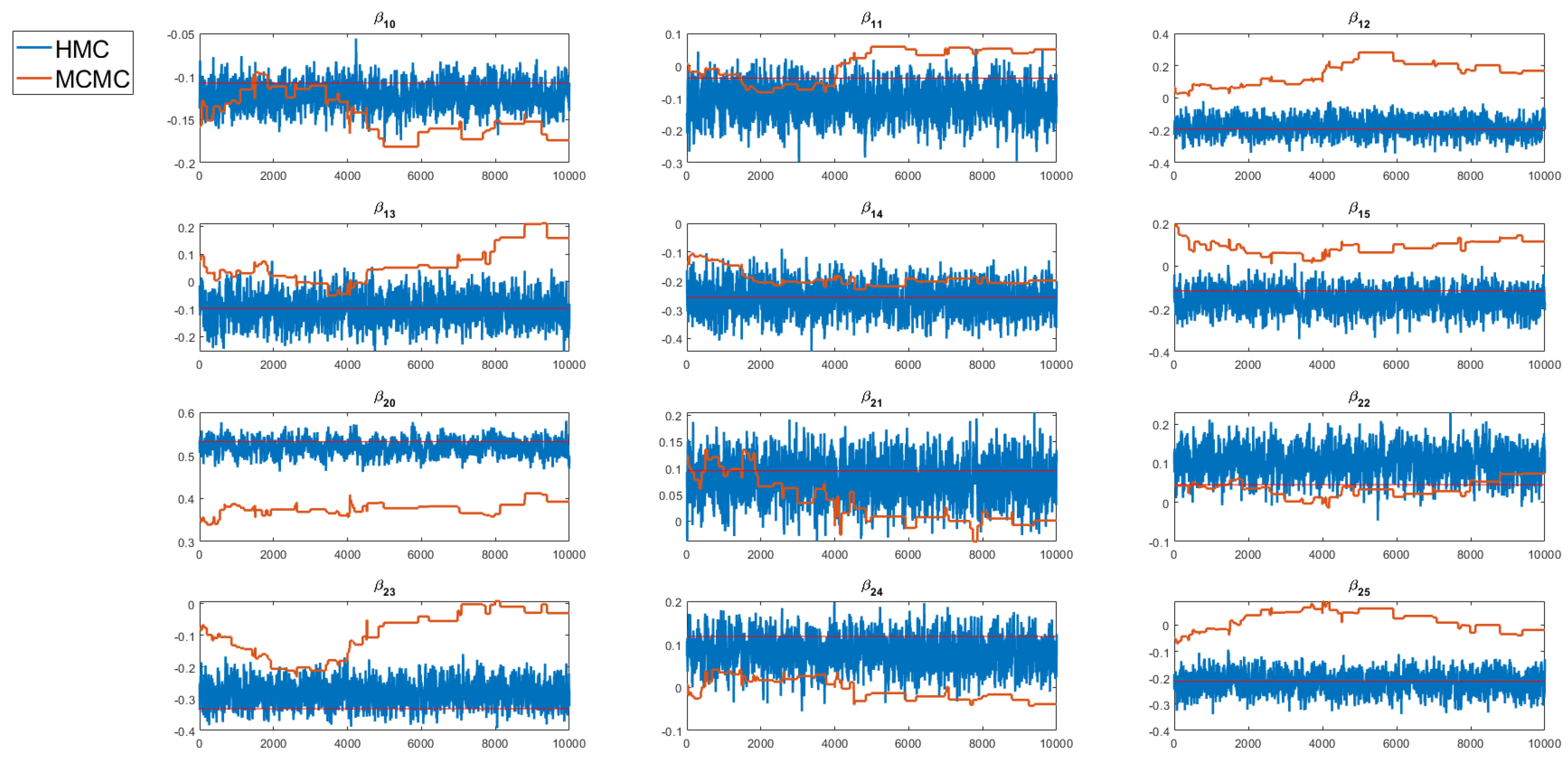
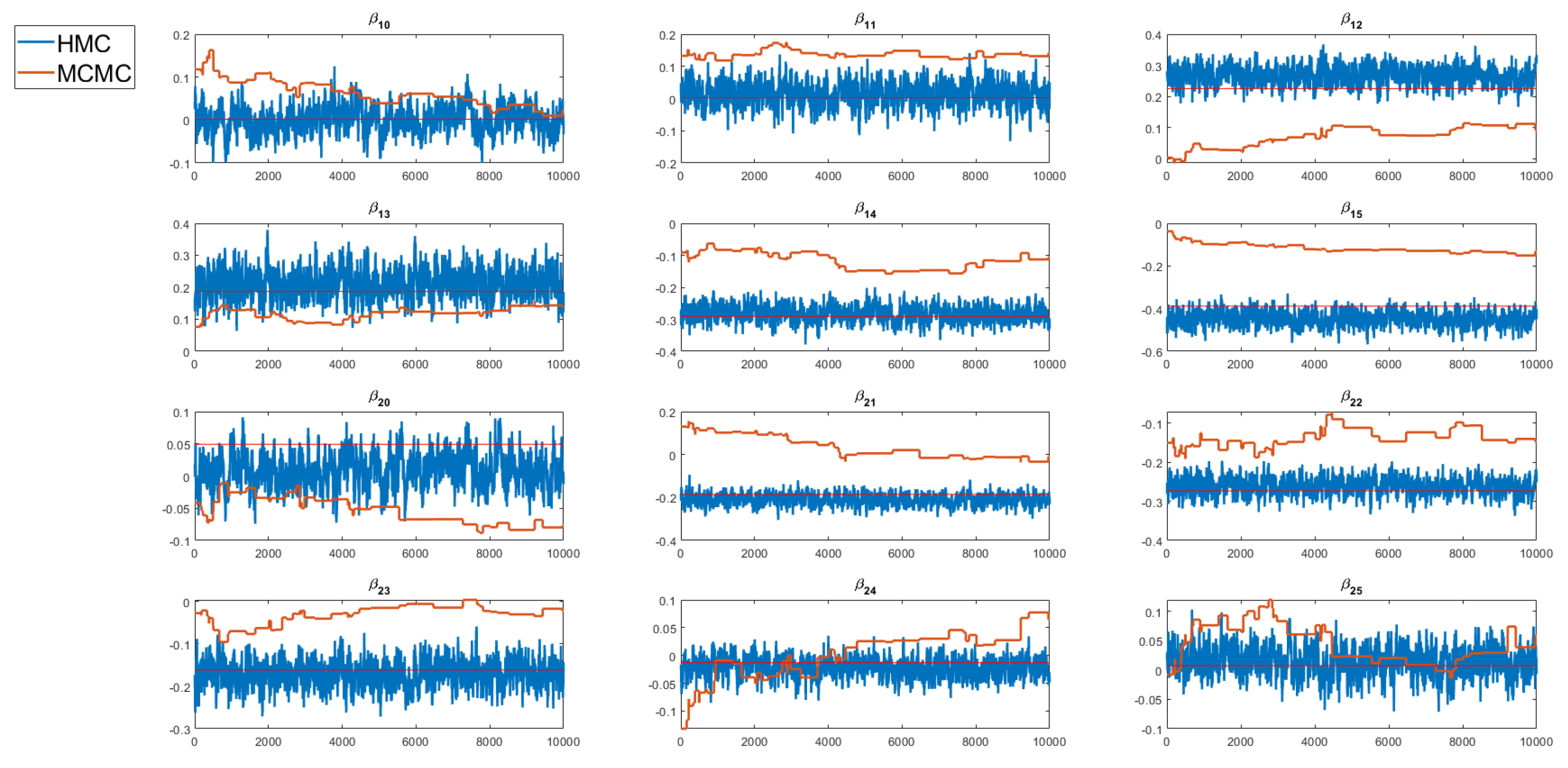
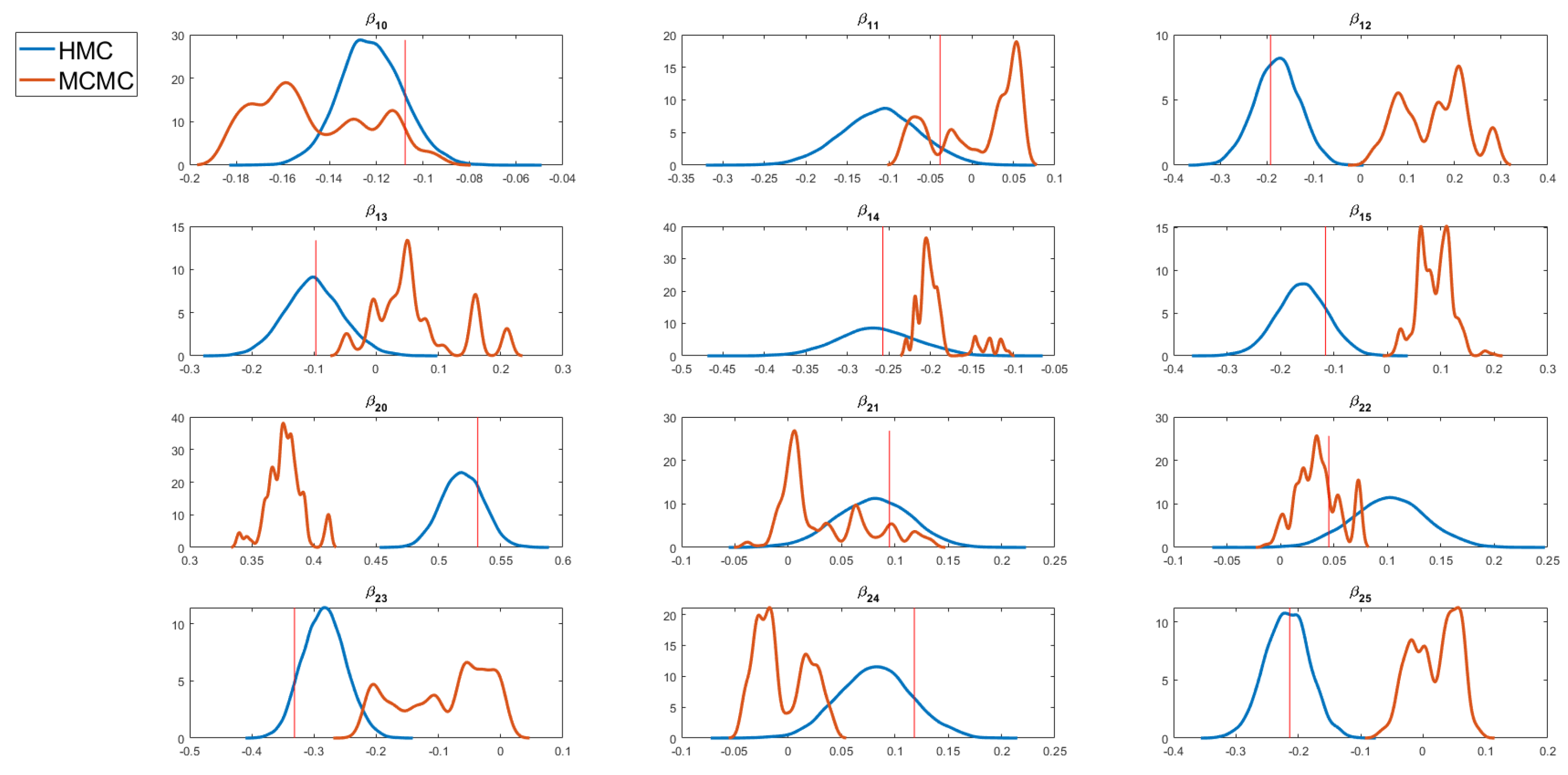
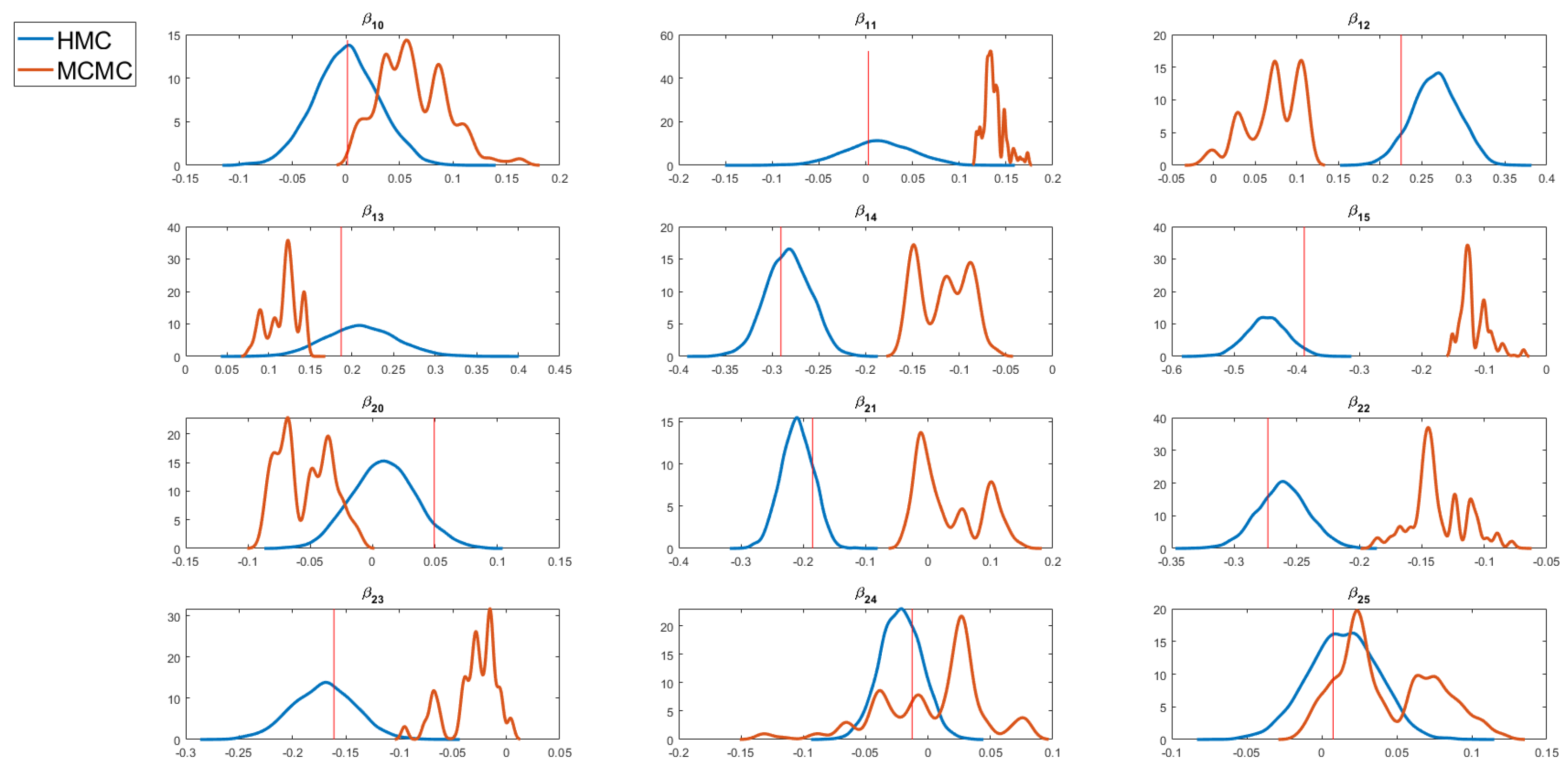
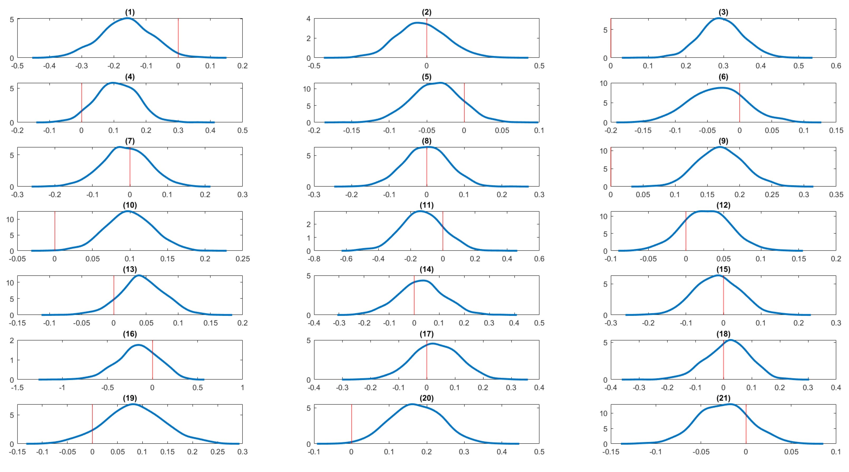
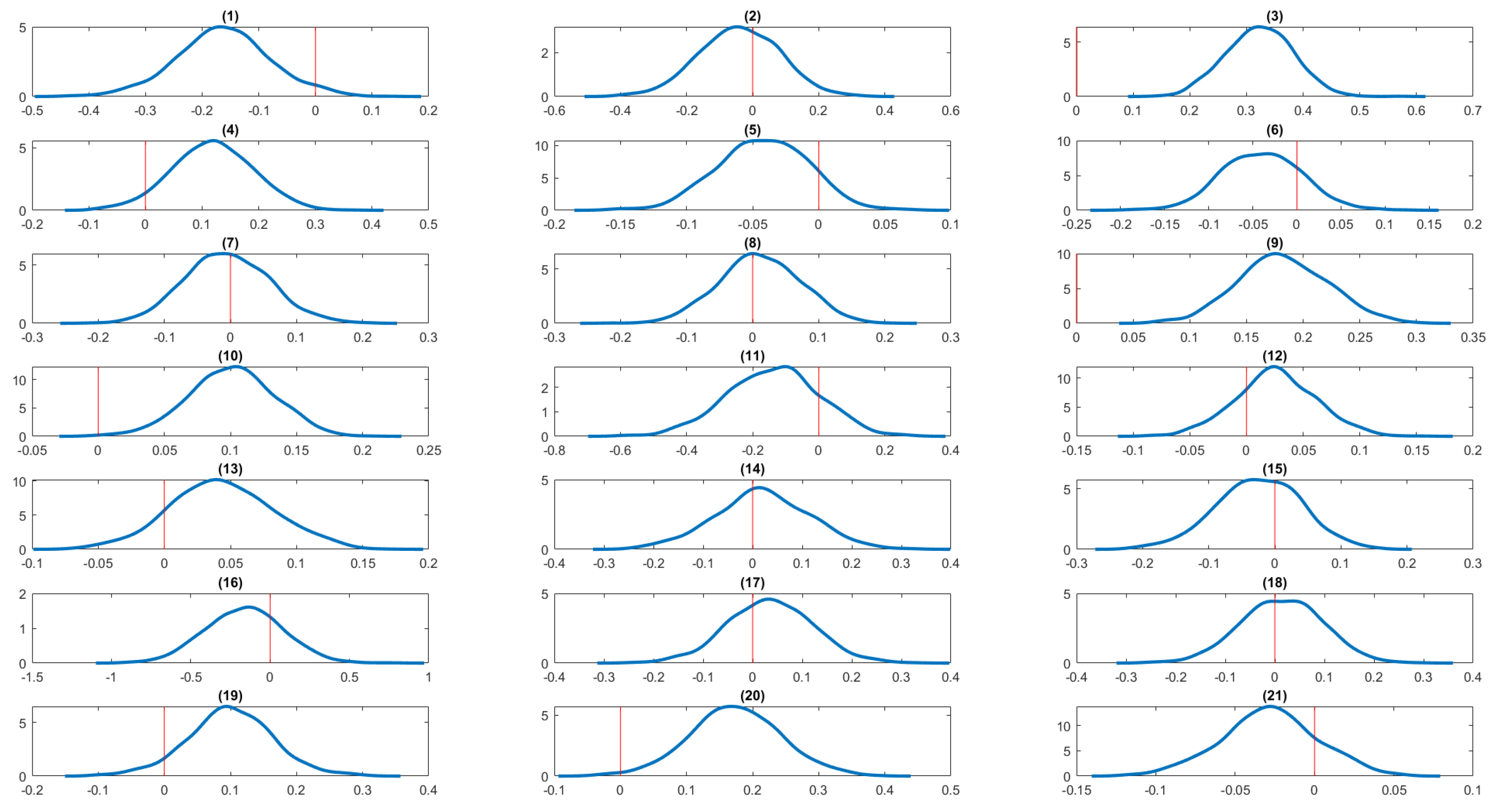
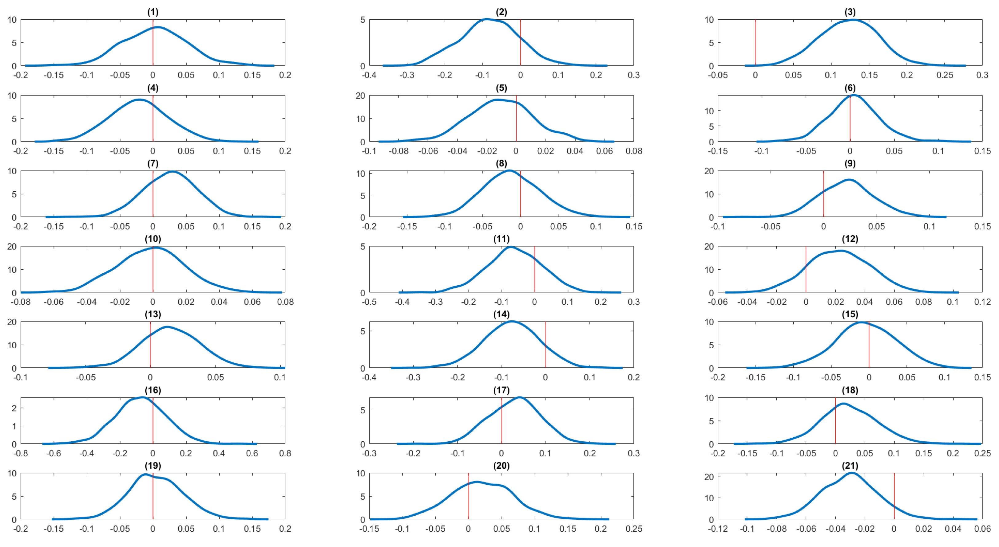
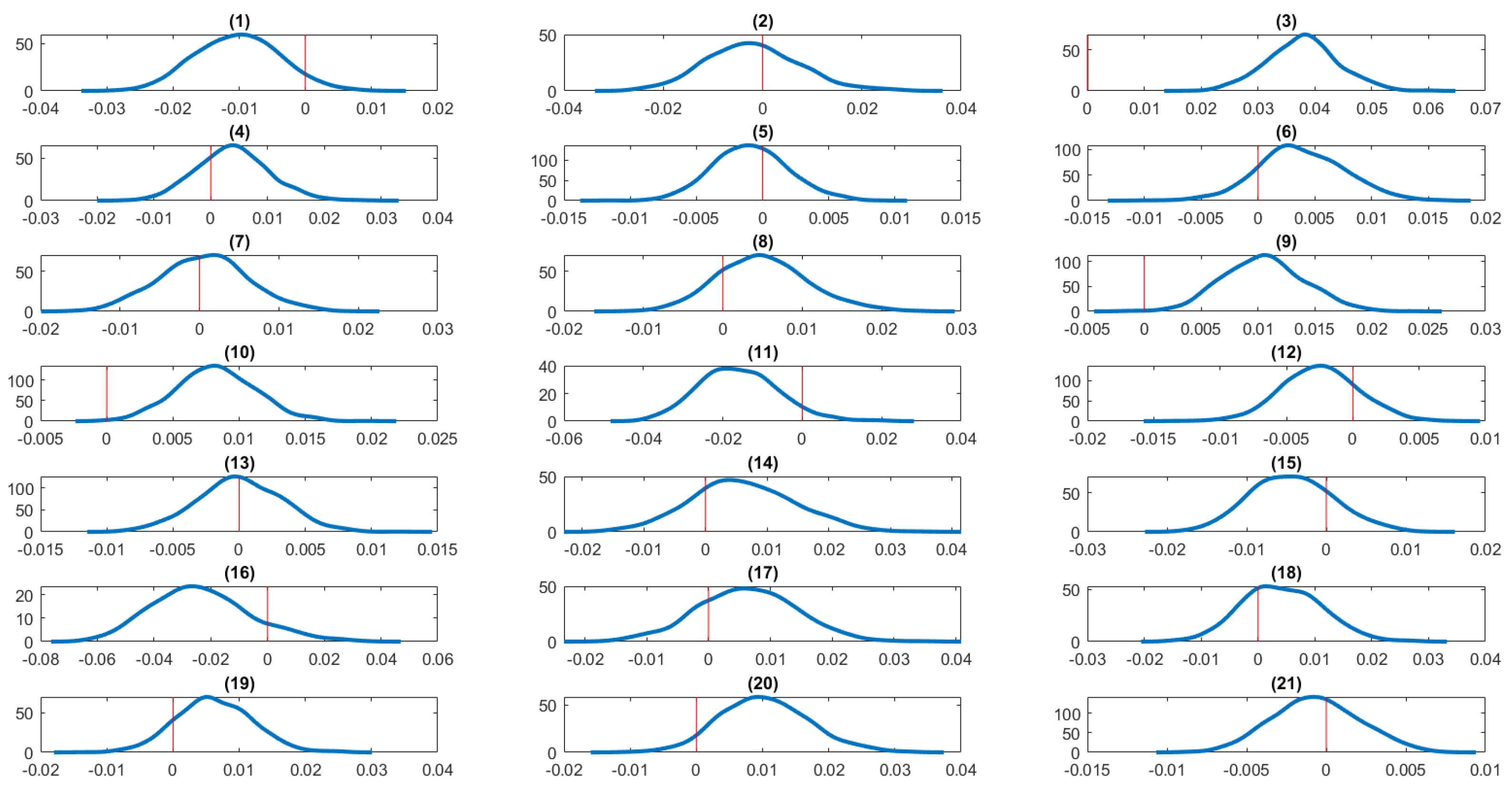
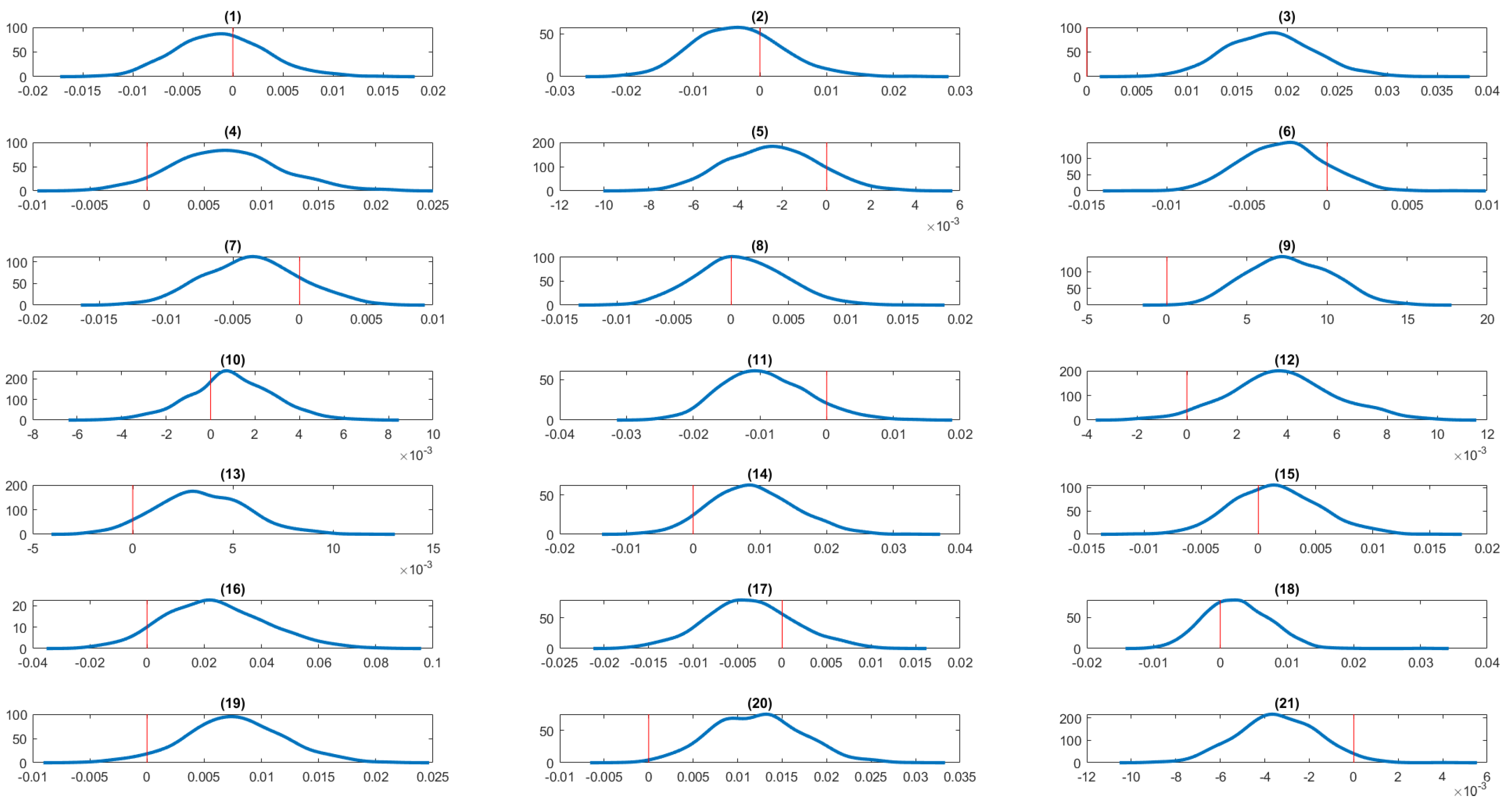
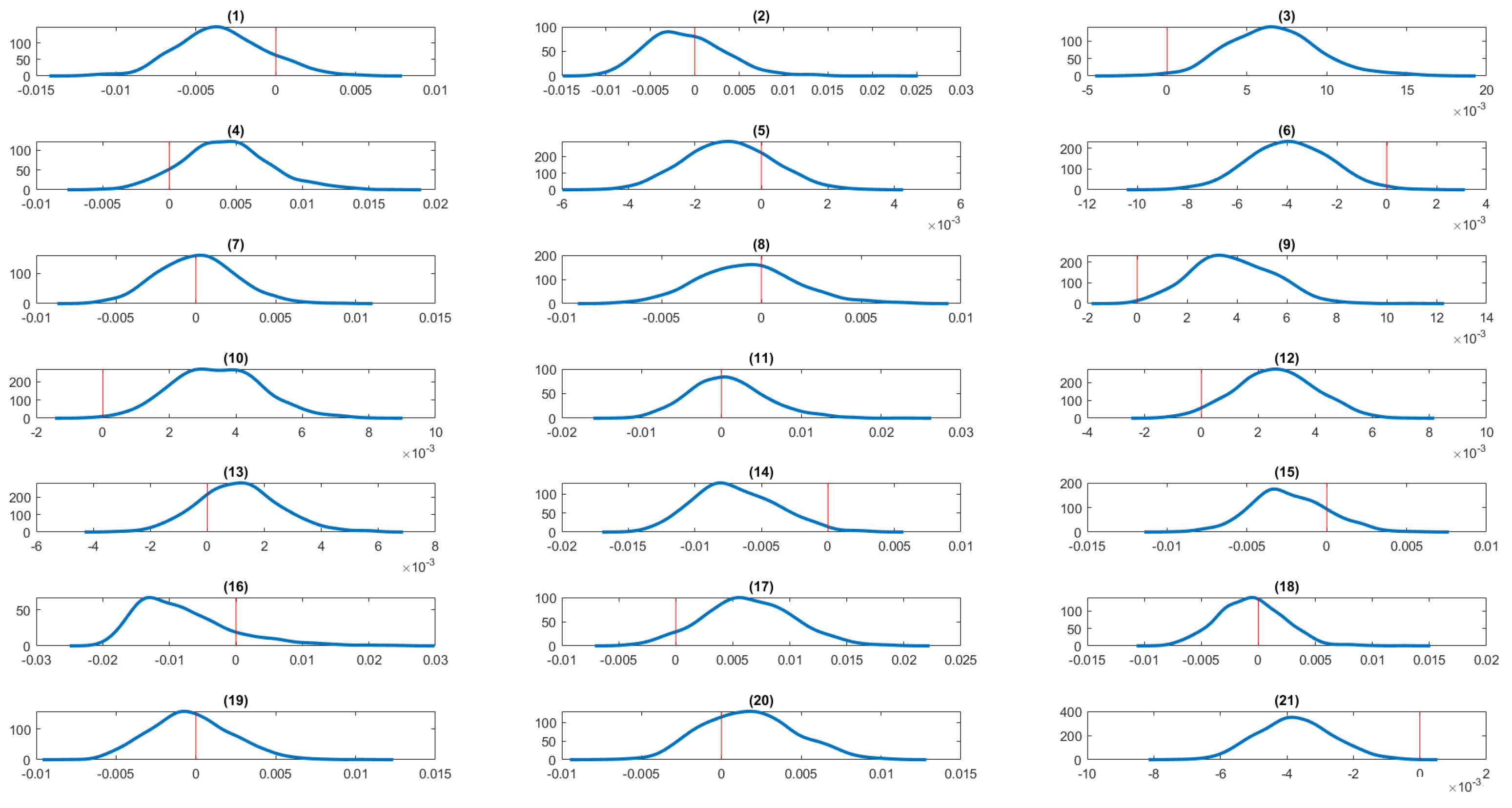
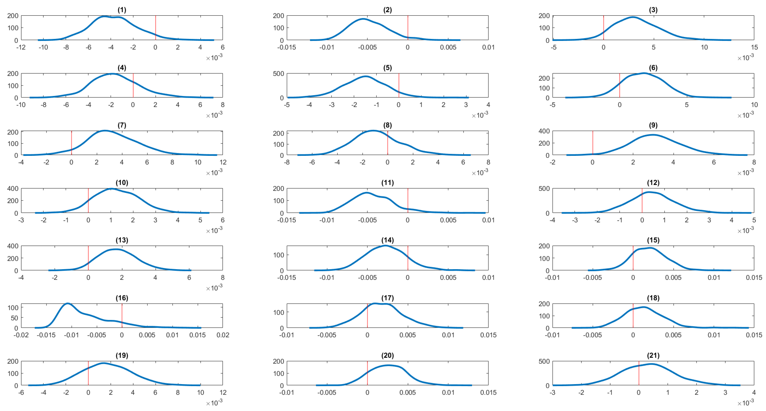
• The PMwG sampler produces well-mixing Markov chains and demonstrates evidence of convergence.
• The PMwG sampler accurately recovers the true regression parameters in high-dimensional settings with 49 continuous and 49 categorical covariates.
• The standard MCMC algorithm exhibits poor mixing and lack of convergence, and fails to recover the true parameter values.

7. Results and Discussion

The PMwG sampling scheme was used to estimate the two longitudinal panel data models defined in Section 3.1 and Section 3.2. For each panel data model, we generated a total of 11,000 posterior samples, of which the first 1000 were discarded as burn-in and every 10th draw of the remaining 10,000 draws were retained. In total, $Q=1000$ iterates of $\mathit{\theta }$ were collected, from which we estimated the posterior means of the model parameters as well as their posterior standard deviations. The posterior means represent point estimates for the regression coefficients and other parameters. The posterior standard deviations reflect the reliability of the point estimates. The posterior draws on the parameters can also be used to plot kernel density estimates of their posterior densities. Bayesian methodology provides information on the entire posterior distribution not only for the parameters of the models but also for other quantities of interest, especially the partial effects. We say that the variable of interest is significant if its $(1-\alpha )100$% credible interval does not include zero. In this paper, we use $\alpha =0.01,0.05,0.1$.

7.1. Main Result

Table 4. Joint posterior probability estimates (90%, 95%, and 99% credible intervals in brackets) of insomnia and obesity ($BMI\ge 25$) obtained from mixed marginal random effects panel data model.

Obesity Classes	Sample Estimates	Mixed Marginal
no insomnia and not obese ($BMI<25$)	0.295	0.287 (0.281, 0.292) (0.280, 0.296) (0.278, 0.297)
insomnia and not obese ($BMI<25$)	0.096	0.090 (0.086, 0.095) (0.085, 0.096) (0.084, 0.097)
no insomnia and obese ($BMI\ge 25$)	0.427	0.435 (0.429, 0.442) (0.426, 0.443) (0.425, 0.447)
insomnia and obese ($BMI\ge 25$)	0.182	0.186 (0.181, 0.192) (0.180, 0.193) (0.179, 0.195)

presents the joint posterior probabilities of insomnia and obesity (defined as $BMI\ge 25$), estimated using a mixed marginal bivariate random effects panel data model, alongside sample estimates for comparison. The results are for the following: (i) no insomnia and not obese, (ii) insomnia and not obese, (iii) no insomnia and obese, and (iv) insomnia and obese. The posterior means are reported with 90%, 95%, and 99% credible intervals. Across all categories, the credible intervals are relatively narrow, indicating high precision in the posterior estimates. The mixed marginal random effects model results are closely aligned with the sample estimates, suggesting that the model captures the joint distribution of insomnia and BMI accurately. The following table shows that the highest joint probability corresponds to individuals who are obese but do not report insomnia, with a posterior mean estimate of $0.435$. The second highest joint probability corresponds to those with neither condition (a posterior mean estimate of $0.287$), followed by individuals with both conditions (a posterior mean estimate of $0.186$). The group with the smallest joint probability estimate is that which experiences insomnia but is not obese, with a posterior mean estimate of $0.090$.

We now examine whether the positive and negative life events discussed in Section 2, experienced by participants, have an effect on insomnia and BMI variables.

Table 5. Effect of positive and negative shocks on insomnia and obesity from the mixed marginal panel data model.

	Dependent Variable
	Insomnia	Obesity	Insomnia	Obesity
Positive events	0.052 0.025 (−0.012, 0.115) ** (0.002, 0.101) (0.010, 0.092)	0.011 0.016 (−0.029, 0.052) (−0.020, 0.041) (−0.016, 0.037)	0.057 0.026 (−0.014, 0.118) ** (0.005, 0.107) (0.015, 0.100)	0.014 0.017 (−0.025, 0.061) (−0.017, 0.047) (−0.013, 0.042)
Negative events	0.088 0.022 (0.033, 0.146) *** (0.049, 0.132) (0.054, 0.124)	0.014 0.013 (−0.018, 0.047) (−0.010, 0.040) (−0.006, 0.036)	0.093 0.022 (0.038, 0.151) *** (0.048, 0.138) (0.055, 0.130)	0.007 0.014 (−0.033, 0.043) (−0.021, 0.034) (−0.016, 0.030)
Individual RE	Yes	Yes	No	No
Individual FE	No	No	Yes	Yes
State FE	Yes	Yes	Yes	Yes
Time FE	Yes	Yes	Yes	Yes

Notes: Posterior standard deviations, 99%, 95%, and 90% credible intervals in parentheses; *** and ** mean that the 99% and 95% credible intervals do not include zero. Control variables described in Section 2 and Section 3 are included.

presents results for the effect of positive and negative life events on insomnia and BMI. Columns (1) and (2) report the results from the mixed marginal panel data model with individual random effects, and columns (3) and (4) report results from the mixed marginal panel data model with individual fixed effects. Each model also controls for state, time-fixed effects, and other control variables described in Section 2 and Section 3. We find that the results of the two models are very similar. Both models show that there are significant positive effects on the probability of insomnia for both positive and negative life events. The negative event coefficient is 1.69 times larger than the positive event coefficient. There are no significant effects for obesity as measured by the BMI.

In

Table 6. Effect of separate shocks on insomnia and obesity from the mixed marginal panel data model.

	Dependent Variable
	Insomnia	Obesity	Insomnia	Obesity
Got married	$-0.163$** (0.078)	0.009 (0.046)	$-0.162$* (0.083)	0.003 (0.048)
Got back together	$-0.121$ (0.110)	$-0.087$ (0.070)	$-0.040$ (0.121)	$-0.082$ (0.077)
Pregnancy	0.294 *** (0.057)	0.110 *** (0.033)	0.323 *** (0.059)	0.123 *** (0.038)
Birth/adoption of new child	0.109 * (0.064)	$-0.010$ (0.041)	0.119 * (0.071)	$-0.121$ (0.044)
Changed jobs	$-0.038$ (0.033)	$-0.018$ (0.019)	$-0.042$ (0.034)	$-0.010$ (0.021)
Promoted at work	$-0.034$ (0.043)	$-0.002$ (0.025)	$-0.040$ (0.046)	0.004 (0.028)
Major improvement in finances	$-0.012$ (0.061)	0.048 (0.037)	$-0.005$ (0.063)	0.026 (0.040)
Separated from spouse	$-0.001$ (0.059)	$-0.022$ (0.036)	0.011 (0.061)	$-0.012$ (0.038)
Serious personal injury or illness	0.170 *** (0.035)	0.049 * (0.024)	0.182 *** (0.039)	0.022 (0.025)
Serious injury/illness to family member	0.099 *** (0.031)	0.000 (0.019)	0.101 *** (0.032)	$-0.001$ (0.020)
Death of spouse/child	$-0.128$ (0.132)	$-0.083$ (0.081)	$-0.139$ (0.138)	$-0.061$ (0.081)
Death of close relative/family member	0.027 (0.032)	0.036 * (0.020)	0.026 (0.035)	0.022 (0.021)
Death of close friend	0.044 (0.035)	0.027 (0.021)	0.043 (0.039)	0.016 (0.022)
Victim of physical violence	0.027 (0.092)	$-0.085$ (0.057)	0.020 (0.095)	$-0.077$ (0.062)
Victim of a property crime	$-0.016$ (0.061)	$-0.009$ (0.036)	$-0.024$ (0.064)	$-0.004$ (0.039)
Detained in jail	$-0.162$ (0.229)	$-0.107$ (0.130)	$-0.162$ (0.244)	$-0.073$ (0.150)
Close family member detained in jail	0.033 (0.082)	0.043 (0.052)	0.035 (0.085)	0.030 (0.057)
Retired from workforce	0.015 (0.077)	0.023 (0.044)	0.014 (0.082)	0.024 (0.048)
Fired or made redundant	0.083 (0.059)	0.018 (0.038)	0.100 (0.064)	0.005 (0.041)
Major worsening in finances	0.172 *** (0.067)	0.039 (0.045)	0.174 ** (0.069)	0.020 (0.046)
Changed residence	$-0.025$ (0.029)	$-0.040$ (0.017)	$-0.028$ (0.030)	$-0.030$ (0.019)
Individual RE	Yes	Yes	No	No
Individual FE	No	No	Yes	Yes
State FE	Yes	Yes	Yes	Yes
Time FE	Yes	Yes	Yes	Yes

Notes: Posterior standard deviations in parentheses; ***, **, and * mean that the 99%, 95%, and 90% credible intervals do not include zero. Control variables described in Section 2 and Section 3 are included.

, we present results for the effects of each serious life event on insomnia and BMI variables. Columns (1) and (2) present results from the mixed marginal panel data model with individual random effects, and columns (3) and (4) present results from the mixed marginal panel data model with individual fixed effects. Each model also controls for state and time-fixed effects and other control variables. Again, the results of the two models are very similar. We now focus on the results from the mixed marginal panel data model with random effects (columns (1) and (2)). Out of the 21 life events analyzed, 6 are statistically significant predictors of insomnia, and 3 are significant for BMI. Specifically, getting married, pregnancy, serious personal injury or illness, serious injury or illness to a family member, birth or adoption of a child, and major worsening in finances are significantly associated with insomnia. For BMI, the significant events are pregnancy, serious personal injury or illness, and the death of a close relative or family member. For insomnia, we find that getting married in the last 12 months reduces the probability of insomnia. In contrast, pregnancy, birth/adoption of a new child, serious personal injury/illness, serious injury/illness to family members, and major worsening in finances in the last 12 months increases the probability of insomnia. For BMI, pregnancy, serious personal injury/illness, and death of a close relative/family member increases the BMI. In addition to reporting posterior means and standard deviations, we also present kernel density estimates of the regression coefficients associated with each serious life event for the insomnia and BMI outcomes. These density estimates provide a visual representation of the posterior distributions and help assess whether the corresponding credible intervals include zero. Figure 6, Figure 7, Figure 8 and Figure 9 display the kernel density estimates of the regression coefficients obtained from the mixed marginal panel data models with both individual random and fixed effects. These figures reinforce the conclusions drawn from the summary statistics reported in the corresponding tables.

7.2. Sensitivity Checks

Across all four tables (

Table 7. Joint posterior probability estimates (90%, 95%, and 99% credible intervals in brackets) of insomnia and overweight obtained from bivariate probit random effects panel data model.

Obesity Classes	Sample Estimates	Bivariate Probit
no insomnia and not overweight	0.474	0.471 (0.466, 0.476) (0.465, 0.477) (0.463, 0.480)
insomnia and not overweight	0.189	0.187 (0.183, 0.191) (0.183, 0.192) (0.181, 0.193)
no insomnia and overweight	0.248	0.252 (0.247, 0.256) (0.247, 0.257) (0.245, 0.259)
insomnia and overweight	0.089	0.090 (0.087, 0.093) (0.086, 0.094) (0.085, 0.095)

,

Table 8. Joint posterior probability estimates (90%, 95%, and 99% credible intervals in brackets) of insomnia and extreme obesity obtained from bivariate probit random effects panel data model.

Obesity Classes	Sample Estimates	Bivariate Probit
no insomnia and not extreme	0.608	0.607 (0.602, 0.612) (0.600, 0.613) (0.599, 0.615)
insomnia and not extreme	0.224	0.224 (0.220, 0.229) (0.219, 0.230) (0.218, 0.232)
no insomnia and extreme	0.114	0.116 (0.112, 0.119) (0.112, 0.120) (0.111, 0.122)
insomnia and extreme	0.0536	0.053 (0.050, 0.056) (0.049, 0.056) (0.048, 0.057)

,

Table 9. Joint posterior probability estimates (90%, 95%, and 99% credible intervals in brackets) of insomnia and severe obesity obtained from bivariate probit random effects panel data model.

Obesity Classes	Sample Estimates	Bivariate Probit
no insomnia and not severe	0.680	0.680 (0.675, 0.684) (0.674, 0.685) (0.672, 0.687)
insomnia and not severe	0.255	0.254 (0.250, 0.259) (0.249, 0.260) (0.248, 0.261)
no insomnia and severe	0.043	0.043 (0.041, 0.045) (0.041, 0.046) (0.040, 0.047)
insomnia and severe	0.0227	0.023 (0.021, 0.025) (0.021, 0.025) (0.020, 0.026)

and

Table 10. Joint posterior probability estimates (90%, 95%, and 99% credible intervals in brackets) of insomnia and very severe obesity obtained from bivariate probit random effects panel data model.

Obesity Classes	Sample Estimates	Bivariate Probit
no insomnia and not very severe	0.700	0.701 (0.697, 0.705) (0.696, 0.706) (0.693, 0.707)
insomnia and not very severe	0.261	0.261 (0.256, 0.265) (0.256, 0.266) (0.253, 0.268)
no insomnia and very severe	0.022	0.022 (0.021, 0.024) (0.021, 0.024) (0.020, 0.025)
insomnia and very severe	0.017	0.016 (0.015, 0.018) (0.015, 0.018) (0.014, 0.018)

), the joint posterior probability estimates of insomnia and different levels of obesity, covering overweight, extreme obesity, severe obesity, and very severe obesity, obtained from the bivariate random effects probit model closely align with the corresponding sample estimates, suggesting that the model fits the data well. For example, in Table 7, the model estimate for the joint probability of insomnia and overweight is $0.090$, nearly identical to the sample estimate of $0.089$. Similarly, close agreement is observed in the other categories and tables. The tight credible intervals around the estimates further underscore their precision and reliability. The tables also show that the joint posterior probability of insomnia and overweight status is estimated at $0.090$, decreasing progressively across higher obesity classes, with the probability for very severe obesity estimated at $0.0167$. These results suggest that while the prevalence of overweight is associated with insomnia, the joint occurrence becomes less frequent as the level of obesity increases.

Table 11. Effect of positive and negative shocks on insomnia and obesity (category overweight) from the bivariate probit panel data model.

	Dependent Variable
	Insomnia	Obesity	Insomnia	Obesity
Positive events	0.052 (0.025) (−0.018, 0.119) (0.002, 0.102) (0.010, 0.095) **	0.115 (0.026) (0.047, 0.183) (0.063, 0.169) (0.073, 0.157) ***	0.058 (0.027) (−0.012, 0.124) (0.003, 0.110) (0.013, 0.104) **	0.106 (0.024) (0.042, 0.166) (0.059, 0.153) (0.068, 0.146) ***
Negative events	0.089 (0.022) (0.032, 0.140) (0.046, 0.130) (0.052, 0.124) ***	−0.016 (0.022) (−0.075, 0.036) (−0.060, 0.027) (−0.054, 0.021)	0.093 (0.023) (0.035, 0.155) (0.048, 0.137) (0.054, 0.130) ***	−0.019 (0.019) (−0.066, 0.032) (−0.056, 0.019) (−0.050, 0.014)
AIC	239,543.88		239,596.67
BIC	240,082.84		240,135.63
Individual RE	Yes	Yes	No	No
Individual FE	No	No	Yes	Yes
State FE	Yes	Yes	Yes	Yes
Time FE	Yes	Yes	Yes	Yes

Notes: Posterior standard deviations, 99%, 95%, and 90% credible intervals in parentheses; *** and ** mean that the 99% and 95% credible intervals do not include zero. Control variables described in Section 2 and Section 3 are included. The table also reports the values of the Akaike Information Criterion (AIC [34]) and the Bayesian Information Criterion (BIC [35]).

,

Table 12. Effect of positive and negative shocks on insomnia and obesity (category extreme) from the bivariate probit panel data model.

	Dependent Variable
	Insomnia	Obesity	Insomnia	Obesity
Positive events	0.053 (0.025) (−0.015, 0.128) (0.004, 0.102) (0.013, 0.094) **	0.015 (0.031) (−0.075, 0.094) (−0.047, 0.077) (−0.034, 0.064)	0.058 (0.027) (−0.009, 0.129) (0.005, 0.111) (0.014, 0.104) **	0.010 (0.029) (−0.068, 0.084) (−0.045, 0.066) (−0.037, 0.056)
Negative events	0.088 (0.022) (0.035, 0.143) (0.045, 0.133) (0.054, 0.125) ***	0.009 (0.025) (−0.050, 0.081) (−0.038, 0.060) (−0.032, 0.052)	0.093 (0.022) (0.038, 0.149) (0.048, 0.135) (0.058, 0.130) ***	0.009 (0.024) (−0.053, 0.067) (−0.036, 0.055) (−0.029, 0.049)
AIC	239,553.68		240,156.83
BIC	240,092.65		240,695.79
Individual RE	Yes	Yes	No	No
Individual FE	No	No	Yes	Yes
State FE	Yes	Yes	Yes	Yes
Time FE	Yes	Yes	Yes	Yes

Notes: Posterior standard deviations, 99%, 95%, and 90% credible intervals in parentheses; *** and ** mean that the 99% and 95% credible intervals do not include zero. Control variables described in Section 2 and Section 3 are included. The table also reports the values of the Akaike Information Criterion (AIC [34]) and the Bayesian Information Criterion (BIC [35]).

,

Table 13. Effect of positive and negative shocks on insomnia and obesity (category severe) from the bivariate probit panel data model.

	Dependent Variable
	Insomnia	Obesity	Insomnia	Obesity
Positive events	0.052 (0.025) (−0.012, 0.117) (0.004, 0.103) (0.012, 0.092) **	−0.037 (0.045) (−0.160, 0.083) (−0.128, 0.045) (−0.113, 0.035)	0.058 (0.027) (−0.008, 0.125) (0.003, 0.113) (0.012, 0.102) **	−0.031 (0.037) (−0.125, 0.060) (−0.101, 0.046) (−0.092, 0.033)
Negative events	0.088 (0.021) (0.033, 0.142) (0.047, 0.130) (0.053, 0.123) ***	0.015 (0.037) (−0.078, 0.108) (−0.055, 0.088) (−0.047, 0.078)	0.093 (0.023) (0.035, 0.151) (0.050, 0.138) (0.056, 0.131) ***	0.016 (0.031) (−0.069, 0.093) (−0.047, 0.078) (−0.037, 0.068)
AIC	241,033.23		242,887.37
BIC	241,572.20		243,426.33
Individual RE	Yes	Yes	No	No
Individual FE	No	No	Yes	Yes
State FE	Yes	Yes	Yes	Yes
Time FE	Yes	Yes	Yes	Yes

Notes: Posterior standard deviations, 99%, 95%, and 90% credible intervals in parentheses; *** and ** mean that the 99% and 95% credible intervals do not include zero. Control variables described in Section 2 and Section 3 are included. The table also reports the values of the Akaike Information Criterion (AIC [34]) and the Bayesian Information Criterion (BIC [35]).

and

Table 14. Effect of positive and negative shocks on insomnia and obesity (category very severe) from the bivariate probit panel data model.

	Dependent Variable
	Insomnia	Obesity	Insomnia	Obesity
Positive events	0.053 (0.025) (−0.006, 0.117) (0.004, 0.102) (0.013, 0.093) **	−0.092 (0.075) (−0.290, 0.102) (−0.245, 0.049) (−0.221, 0.028)	0.058 (0.028) (−0.013, 0.133) (0.003, 0.113) (0.014, 0.101) **	−0.066 (0.047) (−0.197, 0.062) (−0.152, 0.033) (−0.141, 0.015)
Negative events	0.088 (0.022) (0.025, 0.142) (0.043, 0.130) (0.051, 0.124) ***	0.177 (0.065) (0.008, 0.358) (0.057, 0.301) (0.073, 0.279) ***	0.093 (0.022) (0.036, 0.145) (0.051, 0.137) (0.057, 0.131) ***	0.131 (0.039) (0.022, 0.228) (0.056, 0.208) (0.069, 0.195) ***
AIC	240,331.80		246,848.56
BIC	240,870.76		247,387.52
Individual RE	Yes	Yes	No	No
Individual FE	No	No	Yes	Yes
State FE	Yes	Yes	Yes	Yes
Time FE	Yes	Yes	Yes	Yes

Notes: Posterior standard deviations, 99%, 95%, and 90% credible intervals in parentheses; *** and ** mean that the 99% and 95% credible intervals do not include zero. Control variables described in Section 2 and Section 3 are included. The table also reports the values of the Akaike Information Criterion (AIC [34]) and the Bayesian Information Criterion (BIC [35]).

examine the sensitivity of our results across different categories of obesity, as defined in Section 2: overweight, extreme obesity, severe obesity, and very severe obesity. Each model includes state and time-fixed effects, as well as a set of control variables. For the extreme and severe obesity categories, we find that both positive and negative life events are associated with a higher probability of experiencing insomnia, but they have no significant effect on the probability of obesity. In contrast, for the overweight and very severe obesity categories, positive and negative life events increase the likelihood of insomnia, consistent with the other categories. However, the relationship between life events and obesity differs by severity. For the overweight category, positive life events are associated with a higher probability of being overweight. For the very severe obesity category, negative life events are linked to an increased probability of obesity.

In

Table 15. Effect of separate shocks on insomnia and obesity (overweight and extreme categories) from the bivariate probit panel data model.

	Dependent Variable
	Overweight		Extreme
	Insomnia	Obesity	Insomnia	Obesity
Got married	$-0.161$ ** (0.079)	$-0.001$ (0.077)	$-0.163$ ** (0.077)	$0.111$ (0.091)
Got back together	$-0.038$ (0.104)	$0.005$ (0.119)	$-0.033$ (0.105)	$-0.060$ (0.146)
Pregnancy	$0.295$ *** (0.055)	$0.241$ *** (0.058)	$0.298$ *** (0.055)	$0.152$ ** (0.074)
Birth/adoption of new child	$0.110$ (0.067)	$-0.059$ (0.070)	$0.110$ * (0.064)	$0.070$ (0.089)
Changed jobs	$-0.038$ (0.032)	$0.027$ (0.033)	$-0.039$ (0.032)	$-0.030$ (0.043)
Promoted at work	$-0.034$ (0.042)	$0.104$ (0.043)	$-0.035$ (0.042)	$-0.040$ (0.056)
Major improvement in finances	$-0.011$ (0.062)	$0.020$ (0.064)	$-0.010$ (0.061)	$-0.082$ (0.077)
Separated from spouse	$0.001$ (0.061)	$0.084$ (0.061)	$-0.002$ (0.060)	$0.021$ (0.078)
Serious personal injury or illness	$0.173$ *** (0.037)	$-0.020$ (0.039)	$0.172$ *** (0.039)	$0.037$ (0.046)
Serious injury/illness to family member	$0.102$ *** (0.031)	$0.023$ (0.033)	$0.101$ *** (0.031)	$-0.060$ (0.038)
Death of spouse/child	$-0.125$ (0.127)	$-0.160$ (0.138)	$-0.128$ (0.125)	$-0.147$ (0.154)
Death of close relative/family member	$0.025$ (0.034)	$-0.070$ ** (0.035)	$0.024$ (0.034)	$0.072$ * (0.040)
Death of close friend	$0.043$ (0.035)	$-0.048$ (0.038)	$0.045$ (0.036)	$0.046$ (0.044)
Victim of physical violence	$0.028$ (0.090)	$0.068$ (0.097)	$0.031$ (0.091)	$0.178$ (0.112)
Victim of a property crime	$-0.015$ (0.061)	$-0.059$ (0.062)	$-0.015$ (0.060)	$0.048$ (0.076)
Detained in jail	$-0.139$ (0.230)	$-0.317$ (0.251)	$-0.118$ (0.211)	$0.621$ ** (0.286)
Close family member detained in jail	$0.035$ (0.081)	$0.062$ (0.090)	$0.034$ (0.081)	$-0.121$ (0.110)
Retired from workforce	$0.016$ (0.076)	$0.051$ (0.078)	$0.017$ (0.080)	$0.043$ (0.094)
Fired or made redundant	$0.085$ (0.060)	$0.007$ (0.064)	$0.085$ (0.061)	$0.106$ (0.078)
Major worsening in finances	$0.170$ *** (0.068)	$-0.022$ (0.071)	$0.170$ ** (0.068)	$0.129$ (0.084)
Changed residence	$-0.023$ (0.028)	$0.016$ (0.031)	$-0.024$ (0.028)	$-0.066$ * (0.039)
AIC	245,726.68		246,281.47
BIC	246,585.65		247,140.44
Individual RE	Yes	Yes	Yes	Yes
State FE	Yes	Yes	Yes	Yes
Time FE	Yes	Yes	Yes	Yes

Notes: Posterior standard deviations in parentheses; ***, **, and * mean that the 99%, 95%, and 90% credible intervals do not include zero. The table also reports the values of the Akaike Information Criterion (AIC [34]) and the Bayesian Information Criterion (BIC [35]).

and

Table 16. Effect of separate shocks on insomnia and obesity (severe and very severe categories) from the bivariate probit panel data model.

	Dependent Variable
	Severe		Very Severe
	Insomnia	Obesity	Insomnia	Obesity
Got married	$-0.159$ ** (0.078)	$-0.070$ (0.132)	$-0.158$ ** (0.078)	$-0.325$ (0.262)
Got back together	$-0.037$ (0.105)	$-0.038$ (0.193)	$-0.032$ (0.107)	$-0.602$ * (0.333)
Pregnancy	$0.292$ *** (0.054)	$0.090$ (0.097)	$0.293$ *** (0.056)	$0.069$ (0.185)
Birth/adoption of new child	$0.113$ * (0.069)	$0.102$ (0.117)	$0.111$ (0.067)	$-0.280$ (0.229)
Changed jobs	$-0.039$ (0.031)	$-0.021$ (0.057)	$-0.037$ (0.033)	$-0.137$ (0.102)
Promoted at work	$-0.036$ (0.042)	$-0.163$ ** (0.079)	$-0.035$ (0.041)	$0.205$ (0.138)
Major improvement in finances	$-0.011$ (0.061)	$0.006$ (0.101)	$-0.011$ (0.061)	$0.318$ * (0.170)
Separated from spouse	$0.001$ (0.061)	$-0.035$ (0.104)	$-0.001$ (0.060)	$-0.102$ (0.193)
Serious personal injury or illness	$0.173$ *** (0.040)	$0.056$ (0.058)	$0.171$ *** (0.039)	$0.158$ (0.103)
Serious injury/illness to family member	$0.101$ *** (0.030)	$0.085$ * (0.050)	$0.101$ *** (0.030)	$0.043$ (0.094)
Death of spouse/child	$-0.123$ (0.127)	$0.098$ (0.200)	$-0.132$ (0.128)	$-0.453$ (0.343)
Death of close relative/family member	$0.025$ (0.033)	$0.096$ * (0.053)	$0.024$ (0.032)	$0.025$ (0.095)
Death of close friend	$0.043$ (0.035)	$0.021$ (0.057)	$0.042$ (0.036)	$0.139$ (0.104)
Victim of physical violence	$0.032$ (0.091)	$-0.380$ ** (0.175)	$0.033$ (0.089)	$-0.356$ (0.299)
Victim of a property crime	$-0.015$ (0.060)	$-0.105$ (0.108)	$-0.015$ (0.060)	$0.203$ (0.193)
Detained in jail	$-0.134$ (0.226)	$-0.429$ (0.430)	$-0.127$ (0.219)	$-1.157$ (0.890)
Close family member detained in jail	$0.035$ (0.082)	$0.227$ * (0.131)	$0.035$ (0.081)	$0.136$ (0.232)
Retired from workforce	$0.013$ (0.077)	$-0.042$ (0.121)	$0.018$ (0.077)	$0.103$ (0.221)
Fired or made redundant	$0.082$ (0.059)	$-0.066$ (0.105)	$0.084$ (0.059)	$0.090$ (0.194)
Major worsening in finances	$0.172$ *** (0.065)	$-0.031$ (0.109)	$0.171$ *** (0.066)	$0.100$ (0.193)
Changed residence	$-0.025$ (0.028)	$-0.159$ *** (0.051)	$-0.024$ (0.029)	$0.052$ (0.088)
AIC	248,405.39		249,134.30
BIC	249,264.36		249,993.27
Individual RE	Yes	Yes	Yes	Yes
State FE	Yes	Yes	Yes	Yes
Time FE	Yes	Yes	Yes	Yes

Notes: Posterior standard deviations in parentheses; ***, **, and * mean that the 99%, 95%, and 90% credible intervals do not include zero. The table also reports the values of the Akaike Information Criterion (AIC [34]) and the Bayesian Information Criterion (BIC [35]).

, we present results for the effects of each serious life event on insomnia and different levels of obesity variables. Each model controls for the state, time-fixed effects, and other control variables. First, we look at the effect of each life event on insomnia. The results are consistent for different obesity levels. Being married in the past 12 months reduces the probability of insomnia. Pregnancy, serious personal injury/illness, serious injury/illness to family members, and major worsening in finances increase the probability of insomnia. For an overweight level of obesity, pregnancy in the past 12 months increases the probability of being overweight, and the death of a close relative/family member in the past 12 months decreases the probability of being overweight. For the extreme level of obesity, pregnancy, death of a close relative/family, and being detained in jail in the past 12 months increases the probability of being extreme obesity, and changing residence in the past 12 months decreases the probability of being extreme obesity. For a severe level of obesity, being promoted at work, being a victim of physical violence, and changing residence in the past 12 months decrease the probability of being severe obesity, and the death of a close relative/family member, close family member detained in jail, and serious injury/illness to a family member increase the probability of being severe obesity. Finally, for the very severe level of obesity, getting back together with the spouse for the past 12 months reduces the probability of being very severely obese, and a major improvement in finances increases the probability of being very severely obese. Figure 10, Figure 11, Figure 12 and Figure 13 display the kernel density estimates of the regression coefficients obtained from the bivariate random effects probit panel data model. These figures confirm the conclusions drawn from the summary statistics reported in the corresponding tables.

7.3. Average Partial Effects

We use the average partial effect (APE) defined in Section 5 to study how a life event, such as being a victim of a crime, impacts the association between the joint outcomes of insomnia and obesity. We use different levels of obesity: overweight, extreme obesity, severe obesity, and very severe obesity.

Table 17. Average partial effects for the probability of insomnia and obesity (categories: overweight, extreme, severe, and very severe) for major life event variables from the bivariate probit panel data model.

	Average Partial Effects
	Overweight	Extreme	Severe	Very Severe
Got married	$-0.010$ * (0.006)	$-0.001$ (0.004)	$-0.003$ (0.003)	$-0.004$ * (0.002)
Got back together	$-0.002$ (0.009)	$-0.003$ (0.007)	$-0.001$ (0.004)	$-0.005$ * (0.002)
Pregnancy	$0.038$ *** (0.006)	$0.018$ *** (0.004)	$0.007$ ** (0.003)	$0.003$ (0.002)
Birth/adoption of new child	$0.004$ (0.006)	$0.007$ (0.005)	$0.004$ (0.003)	$-0.002$ (0.002)
Changed jobs	$-0.001$ (0.003)	$-0.002$ (0.002)	$-0.001$ (0.001)	$-0.002$ (0.001)
Promoted at work	$0.004$ (0.004)	$-0.003$ (0.003)	$-0.004$ ** (0.002)	$0.002$ (0.001)
Major improvement in finances	$0.001$ (0.006)	$-0.004$ (0.004)	$0.000$ (0.002)	$0.003$ (0.002)
Separated from spouse	$0.005$ (0.006)	$0.001$ (0.004)	$-0.001$ (0.002)	$-0.001$ (0.002)
Serious personal injury or illness	$0.010$ *** (0.004)	$0.008$ *** (0.003)	$0.004$ *** (0.002)	$0.003$ ** (0.001)
Serious injury/illness to family member	$0.008$ *** (0.003)	$0.001$ (0.002)	$0.003$ *** (0.001)	$0.001$ (0.001)
Death of spouse/child	$-0.016$ (0.010)	$-0.009$ (0.006)	$0.001$ (0.005)	$-0.004$ (0.003)
Death of close relative/family member	$-0.002$ (0.003)	$0.004$ * (0.002)	$0.003$ * (0.001)	$0.000$ (0.001)
Death of close friend	$0.000$ (0.003)	$0.003$ (0.002)	$0.001$ (0.001)	$0.002$ * (0.001)
Victim of physical violence	$0.006$ (0.008)	$0.009$ (0.006)	$-0.007$ ** (0.003)	$-0.003$ (0.002)
Victim of a property crime	$-0.004$ (0.005)	$0.002$ (0.004)	$-0.002$ (0.002)	$0.002$ (0.002)
Detained in jail	$-0.023$ (0.017)	$0.024$ (0.018)	$-0.008$ (0.007)	$-0.007$ (0.005)
Close family member detained in jail	$0.006$ (0.008)	$-0.004$ (0.005)	$0.006$ (0.004)	$0.002$ (0.003)
Retired from workforce	$0.004$ (0.007)	$0.003$ (0.005)	$-0.001$ (0.003)	$0.001$ (0.002)
Fired or made redundant	$0.006$ (0.006)	$0.008$ * (0.004)	$-0.000$ (0.003)	$0.002$ (0.002)
Major worsening in finances	$0.010$ (0.007)	$0.012$ *** (0.005)	$0.002$ (0.003)	$0.003$ (0.002)
Changed residence	$-0.001$ (0.003)	$-0.003$ * (0.002)	$-0.004$ *** (0.001)	$0.000$ (0.001)
Individual RE	Yes	Yes	Yes	Yes
State FE	Yes	Yes	Yes	Yes
Time FE	Yes	Yes	Yes	Yes

Notes: Posterior standard deviations in parentheses; ***, **, and * mean that the 99%, 95%, and 90% credible intervals do not include zero. Control variables described in Section 2 and Section 3 are included.

summarizes the estimates of the APEs for major life event shocks for the probability of insomnia and different levels of obesity for the bivariate probit model with random effects. In this case, the sign of the APE provides a clear qualitative interpretation, with a significant positive sign implying a significant increase in the joint probability of insomnia and obesity, and vice versa. We find that the life events that are significant are different for different levels of obesity. For overweight, the effect of getting married $(\mathrm{APE}=-0.010)$ decreases the joint probability of insomnia and being overweight. Pregnancy $(\mathrm{APE}=0.038)$, serious personal injury/illness $(\mathrm{APE}=0.010)$, and serious injury to family member $(\mathrm{APE}=0.008)$ increase the joint probability of insomnia and being overweight.

For the extreme category, several major life events are associated with significant changes in the joint probability of insomnia and obesity. Pregnancy $(\mathrm{APE}=0.018)$, serious personal injury or illness $(\mathrm{APE}=0.008)$, major worsening in finances $(\mathrm{APE}=0.012)$, being fired $(\mathrm{APE}=0.008)$, and death of a close relative or family member $(\mathrm{APE}=0.004)$ increase the probability of insomnia and obesity. In contrast, changed residence $(\mathrm{APE}=-0.003)$ is associated with a significant negative effect.

For the severe category, pregnancy remains a positive and significant factor $(\mathrm{APE}=0.007)$, although the magnitude is smaller. Serious personal injury or illness, serious injury or illness to a family member, and death of a close relative or family member are also significant positive factors $(\mathrm{APE}=0.004,0.003,0.003,\mathrm{respectively})$. Interestingly, promotion at work has a significant negative effect $(\mathrm{APE}=-0.004)$, and being a victim of physical violence $(\mathrm{APE}=-0.007)$ and changed residence $(\mathrm{APE}=-0.004)$ are associated with a significant reduction in the probability.

For the very severe category, fewer life events have statistically significant effects. Serious personal injury or illness and death of a close friend have positive and significant effects $(\mathrm{APE}=0.003,0.002,\mathrm{respectively})$, while both got married and got back together with a partner show significant negative effects $(\mathrm{APE}=-0.004\mathrm{and}-0.005,\mathrm{respectively})$.

In summary, pregnancy, serious personal injury or illness, and financial hardship consistently increase the joint probability of insomnia and obesity across different levels of obesity. Conversely, positive life transitions such as marriage or reconciliation sometimes have significant negative effects, particularly in the very severe category. The influence of negative events appears strongest in the extreme and severe categories, while the very severe category reflects fewer significant impacts overall. Figure 14, Figure 15, Figure 16 and Figure 17 display the kernel density estimates of the average partial effects obtained from the bivariate random effects probit panel data model. These figures confirm the conclusions drawn from the summary statistics reported in the corresponding tables.

7.4. Heterogeneity Analysis

The impact of major life events on the joint probability of insomnia and obesity could potentially be different across subgroups. To examine the sensitivity of our results to different groups, as shown in

Table 18. Average partial effects for the probability of insomnia and obesity (overweight) for major life event variables from the bivariate probit panel data model for different population subgroups.

	Average Partial Effects
	Male	Female	<40	>40	Low	High
Got married	$-0.019$ ** (0.009)	$-0.001$ (0.009)	$-0.009$ (0.007)	$-0.020$ (0.012)	$-0.005$ (0.009)	$-0.019$ *** (0.009)
Got back together	$0.006$ (0.017)	$-0.006$ (0.013)	$-0.008$ (0.011)	$0.016$ (0.021)	$-0.001$ (0.012)	$0.005$ (0.022)
Pregnancy	$0.006$ (0.008)	$0.062$ *** (0.009)	$0.041$ *** (0.007)	$-0.008$ (0.016)	$0.026$ *** (0.008)	$0.055$ *** (0.011)
Birth/adoption of new child	$0.020$ ** (0.010)	$-0.012$ (0.007)	$0.002$ (0.006)	$0.023$ (0.024)	$-0.004$ (0.008)	$0.014$ (0.010)
Changed jobs	$-0.000$ (0.004)	$-0.000$ (0.004)	$-0.001$ (0.003)	$-0.001$ (0.005)	$0.001$ (0.004)	$-0.006$ (0.005)
Promoted at work	$0.004$ (0.006)	$0.005$ (0.005)	$0.007$ (0.005)	$0.000$ (0.008)	$0.005$ (0.005)	$0.001$ (0.006)
Major improvement in finances	$0.009$ (0.009)	$-0.007$ (0.007)	$0.000$ (0.008)	$0.000$ (0.007)	$0.003$ (0.007)	$-0.002$ (0.008)
Separated from spouse	$0.006$ (0.009)	$0.002$ (0.007)	$0.008$ (0.007)	$-0.008$ (0.009)	$0.003$ (0.006)	$0.013$ (0.012)
Serious personal injury or illness	$0.010$ ** (0.005)	$0.013$ *** (0.005)	$0.011$ * (0.006)	$0.012$ ** (0.005)	$0.009$ ** (0.004)	$0.014$ ** (0.006)
Serious injury/illness to family member	$0.005$ (0.004)	$0.009$ ** (0.004)	$0.010$ ** (0.005)	$0.007$ * (0.004)	$0.006$ * (0.004)	$0.009$ * (0.005)
Death of spouse/child	$-0.019$ (0.018)	$-0.012$ (0.013)	$-0.012$ (0.020)	$-0.019$ (0.013)	$-0.013$ (0.012)	$-0.028$ (0.017)
Death of close relative/family member	$-0.004$ (0.005)	$-0.001$ (0.004)	$-0.002$ (0.004)	$-0.003$ (0.004)	$-0.002$ (0.003)	$-0.004$ (0.005)
Death of close friend	$0.001$ (0.005)	$-0.001$ (0.004)	$0.009$ * (0.006)	$-0.004$ (0.004)	$0.000$ (0.004)	$0.000$ (0.006)
Victim of physical violence	$0.021$ (0.015)	$-0.004$ (0.011)	$-0.001$ (0.010)	$0.018$ (0.017)	$-0.001$ (0.009)	$0.031$ (0.023)
Victim of a property crime	$0.001$ (0.008)	$-0.009$ (0.007)	$0.001$ (0.007)	$-0.018$ ** (0.007)	$-0.004$ (0.007)	$-0.007$ (0.008)
Detained in jail	$-0.028$ (0.019)	$-0.005$ (0.037)	$-0.032$ (0.018)	$-0.019$ (0.029)	$-0.021$ (0.017)	$-0.092$ *** (0.005)
Close family member detained in jail	$0.014$ (0.014)	$0.003$ (0.010)	$0.006$ (0.010)	$0.011$ (0.012)	$0.006$ (0.009)	$0.003$ (0.015)
Retired from workforce	$0.012$ (0.011)	$-0.002$ (0.009)	$0.043$ (0.033)	$0.001$ (0.008)	$0.003$ (0.008)	$0.008$ (0.015)
Fired or made redundant	$0.002$ (0.008)	$0.014$ (0.009)	$0.002$ (0.007)	$0.005$ (0.009)	$0.004$ (0.007)	$0.009$ (0.011)
Major worsening in finances	$0.006$ (0.010)	$0.012$ (0.009)	$0.014$ (0.010)	$0.005$ (0.009)	$0.020$ *** (0.008)	$-0.008$ (0.011)
Changed residence	−0.002 (0.004)	0.001 (0.003)	−0.000 (0.003)	−0.002 (0.005)	0.000 (0.003)	−0.002 (0.004)
Individual RE	Yes	Yes	Yes	Yes	Yes	Yes
State FE	Yes	Yes	Yes	Yes	Yes	Yes
Time FE	Yes	Yes	Yes	Yes	Yes	Yes

Notes: Posterior standard deviations in parentheses; ***, **, and * mean that the 99%, 95%, and 90% credible intervals do not include zero. Control variables described in Section 2 and Section 3 are included.

,

Table 19. Average partial effects for the probability of insomnia and obesity (extreme) for major life event variables from the bivariate probit panel data model for different population subgroups.

	Average Partial Effects
	Male	Female	<40	>40	Low	High
Got married	−0.002 (0.006)	−0.002 (0.007)	−0.006 (0.005)	0.023 * (0.012)	0.005 (0.007)	−0.007 (0.006)
Got back together	0.001 (0.010)	−0.003 (0.010)	−0.007 (0.007)	0.012 (0.015)	−0.002 (0.008)	−0.001 (0.014)
Pregnancy	0.002 (0.005)	0.033 *** (0.007)	0.017 *** (0.004)	−0.003 (0.011)	0.018 *** (0.006)	0.013 ** (0.006)
Birth/adoption of new child	0.008 (0.006)	0.004 (0.007)	0.004 (0.004)	0.033 * (0.020)	0.004 (0.006)	0.013 ** (0.007)
Changed jobs	−0.002 (0.003)	−0.003 (0.003)	−0.002 (0.002)	−0.004 (0.004)	−0.001 (0.003)	−0.003 (0.003)
Promoted at work	−0.003 (0.003)	−0.002 (0.004)	−0.004 (0.003)	0.007 (0.006)	−0.002 (0.004)	−0.003 (0.003)
Major improvement in finances	−0.003 (0.005)	−0.004 (0.005)	−0.003 (0.005)	−0.006 (0.005)	−0.002 (0.005)	−0.005 (0.005)
Separated from spouse	0.004 (0.006)	−0.003 (0.005)	0.004 (0.005)	−0.005 (0.006)	0.004 (0.005)	−0.009 (0.006)
Serious personal injury or illness	0.011 *** (0.004)	0.004 (0.004)	0.009 ** (0.004)	0.007 ** (0.003)	0.008 ** (0.003)	0.006 (0.004)
Serious injury/illness to family member	−0.002 (0.003)	0.003 (0.003)	0.001 (0.003)	0.000 (0.003)	0.003 (0.003)	−0.002 (0.003)
Death of spouse/child	−0.008 (0.011)	−0.010 (0.009)	−0.008 (0.012)	−0.010 (0.009)	−0.009 (0.009)	−0.010 (0.011)
Death of close relative/family member	0.004 (0.003)	0.004 (0.003)	0.001 (0.003)	0.006 ** (0.003)	0.004 * (0.003)	0.003 (0.003)
Death of close friend	0.005 (0.003)	0.002 (0.003)	0.004 (0.004)	0.004 (0.003)	0.003 (0.003)	0.004 (0.004)
Victim of physical violence	0.013 (0.009)	0.006 (0.009)	0.007 (0.007)	0.017 (0.013)	0.007 (0.007)	0.017 (0.013)
Victim of a property crime	0.007 (0.005)	−0.004 (0.005)	0.003 (0.005)	−0.001 (0.006)	0.001 (0.005)	0.002 (0.005)
Detained in jail	0.019 (0.019)	0.031 (0.010)	0.008 (0.018)	0.068 ** (0.040)	0.014 (0.017)	0.172 ** (0.104)
Close family member detained in jail	−0.007 (0.007)	−0.000 (0.007)	−0.021 *** (0.005)	0.015 * (0.009)	−0.007 (0.006)	0.007 (0.010)
Retired from workforce	0.002 (0.006)	0.003 (0.007)	0.015 (0.023)	0.001 (0.005)	0.000 (0.006)	0.006 (0.009)
Fired or made redundant	0.009 * (0.005)	0.005 (0.007)	0.006 (0.005)	0.006 (0.006)	0.013 *** (0.005)	−0.004 (0.006)
Major worsening in finances	0.009 (0.007)	0.013 * (0.007)	0.012 * (0.007)	0.010 (0.0007)	0.016 *** (0.006)	0.006 (0.007)
Changed residence	−0.004 (0.003)	−0.003 (0.003)	−0.005 ** (0.002)	0.001 (0.003)	−0.002 (0.002)	−0.005 ** (0.003)
Individual RE	Yes	Yes	Yes	Yes	Yes	Yes
State FE	Yes	Yes	Yes	Yes	Yes	Yes
Time FE	Yes	Yes	Yes	Yes	Yes	Yes

Notes: Posterior standard deviations in parentheses; ***, **, and * mean that the 99%, 95%, and 90% credible intervals do not include zero. Control variables described in Section 2 and Section 3 are included.

,

Table 20. Average partial effects for the probability of insomnia and obesity (severe) for major life event variables from the bivariate probit panel data model for different population subgroups.

	Average Partial Effects
	Male	Female	<40	>40	Low	High
Got married	−0.002 (0.003)	−0.004 (0.005)	−0.002 (0.003)	−0.004 (0.006)	0.001 (0.004)	−0.007 ** (0.003)
Got back together	−0.006 (0.004)	0.005 (0.008)	−0.004 (0.005)	0.007 (0.010)	−0.005 (0.005)	0.022 * (0.015)
Pregnancy	−0.001 (0.002)	0.016 *** (0.005)	0.006 ** (0.003)	−0.009 (0.006)	0.010 ** (0.004)	−0.001 (0.004)
Birth/adoption of new child	0.005 (0.004)	0.004 (0.005)	0.003 (0.003)	0.020 (0.017)	0.004 (0.004)	0.005 (0.005)
Changed jobs	−0.001 (0.001)	−0.001 (0.002)	0.002 (0.002)	−0.003 (0.002)	−0.002 (0.002)	0.001 (0.002)
Promoted at work	−0.003 (0.002)	−0.005 (0.003)	−0.003 (0.002)	−0.002 (0.003)	−0.002 (0.003)	−0.005 *** (0.002)
Major improvement in finances	0.002 (0.003)	−0.003 (0.004)	−0.005 (0.003)	−0.000 (0.003)	−0.001 (0.004)	0.002 (0.003)
Separated from spouse	−0.004 (0.003)	0.002 (0.004)	−0.001 (0.003)	−0.005 (0.004)	0.001 (0.003)	−0.005 (0.004)
Serious personal injury or illness	0.000 (0.002)	0.008 *** (0.003)	0.005 * (0.003)	0.003 (0.002)	0.004 * (0.002)	0.002 (0.002)
Serious injury/illness to family member	0.003 ** (0.002)	0.004 * (0.002)	0.003 (0.002)	0.004 ** (0.002)	0.007 *** (0.002)	−0.001 (0.002)
Death of spouse/child	0.012 (0.010)	−0.004 (0.007)	0.004 (0.010)	−0.001 (0.006)	0.003 (0.006)	−0.007 (0.007)
Death of close relative/family member	0.000 (0.001)	0.005 ** (0.002)	0.005 ** (0.002)	0.001 (0.002)	0.003 (0.002)	0.004 ** (0.002)
Death of close friend	0.000 (0.002)	0.002 (0.002)	0.006 ** (0.003)	−0.000 (0.002)	−0.000 (0.002)	0.004 (0.002)
Victim of physical violence	−0.008 ** (0.003)	−0.006 (0.005)	−0.006 (0.004)	−0.009 (0.005)	−0.009 ** (0.004)	−0.001 (0.008)
Victim of a property crime	−0.001 (0.002)	−0.004 (0.004)	−0.002 (0.003)	−0.004 (0.003)	−0.003 (0.003)	−0.001 (0.003)
Detained in jail	−0.002 (0.006)	−0.025 *** (0.005)	−0.005 (0.008)	−0.021 ** (0.005)	−0.008 (0.008)	−0.013 (0.007)
Close family member detained in jail	0.007 (0.005)	0.006 (0.006)	0.007 (0.005)	0.006 (0.006)	0.009 ** (0.005)	0.000 (0.006)
Retired from workforce	−0.000 (0.003)	−0.001 (0.005)	−0.011 (0.008)	−0.000 (0.003)	−0.001 (0.004)	−0.000 (0.005)
Fired or made redundant	0.000 (0.002)	−0.000 (0.005)	−0.003 (0.003)	0.001 (0.004)	0.001 (0.003)	−0.003 (0.004)
Major worsening in finances	−0.001 (0.003)	0.005 (0.005)	0.001 (0.004)	0.001 (0.004)	0.002 (0.004)	0.004 (0.005)
Changed residence	−0.001 (0.001)	−0.006 *** (0.002)	−0.005 ** (0.001)	−0.002 (0.002)	−0.004 ** (0.002)	−0.005 *** (0.002)
Individual RE	Yes	Yes	Yes	Yes	Yes	Yes
State FE	Yes	Yes	Yes	Yes	Yes	Yes
Time FE	Yes	Yes	Yes	Yes	Yes	Yes

Notes: Posterior standard deviations in parentheses; ***, **, and * mean that the 99%, 95%, and 90% credible intervals do not include zero. Control variables described in Section 2 and Section 3 are included.

and

Table 21. Average partial effects for the probability of insomnia and obesity (very severe) for major life event variables from the bivariate probit panel data model for different population subgroups.

	Average Partial Effects
	Male	Female	<40	>40	Low	High
Got married	−0.001 (0.002)	−0.007 ** (0.003)	−0.004 * (0.002)	−0.003 (0.004)	−0.004 (0.003)	−0.004 * (0.002)
Got back together	−0.000 (0.003)	−0.008 * (0.004)	−0.009 *** (0.002)	0.009 (0.008)	−0.003 (0.004)	−0.008 ** (0.003)
Pregnancy	−0.000 (0.002)	0.009 *** (0.004)	0.003 * (0.002)	−0.002 (0.005)	−0.001 (0.003)	0.007 *** (0.003)
Birth/adoption of new child	0.003 (0.003)	−0.006 * (0.003)	−0.001 (0.002)	0.013 (0.013)	0.004 (0.004)	−0.007 *** (0.001)
Changed jobs	0.000 (0.001)	−0.004 ** (0.002)	−0.002 (0.001)	−0.001 (0.002)	−0.000 (0.001)	−0.004 *** (0.001)
Promoted at work	0.001 (0.002)	0.001 (0.002)	0.002 (0.002)	0.003 (0.003)	0.002 (0.002)	0.001 (0.002)
Major improvement in finances	0.004 * (0.002)	0.002 (0.003)	0.003 (0.003)	0.001 (0.002)	0.006 ** (0.003)	0.001 (0.002)
Separated from spouse	−0.001 (0.002)	−0.001 (0.003)	0.001 (0.002)	−0.007 *** (0.002)	−0.002 (0.002)	0.001 (0.003)
Serious personal injury or illness	0.002 (0.001)	0.005 ** (0.002)	0.002 (0.002)	0.002 (0.002)	0.000 (0.001)	0.008 *** (0.002)
Serious injury/illness to family member	0.001 (0.001)	0.002 (0.002)	0.001 (0.002)	0.001 (0.001)	0.002 (0.001)	0.000 (0.001)
Death of spouse/child	−0.004 (0.004)	−0.006 (0.004)	−0.001 (0.006)	−0.005 (0.003)	−0.004 (0.004)	−0.003 (0.004)
Death of close relative/family member	−0.001 (0.001)	0.002 (0.002)	−0.000 (0.001)	0.001 (0.001)	0.001 (0.001)	0.000 (0.001)
Death of close friend	0.001 (0.001)	0.002 (0.002)	0.002 (0.002)	0.002 (0.001)	0.001 (0.001)	0.003 * (0.002)
Victim of physical violence	−0.002 (0.003)	−0.002 (0.004)	−0.001 (0.004)	−0.001 (0.005)	−0.000 (0.004)	−0.008 *** (0.002)
Victim of a property crime	0.002 (0.002)	0.001 (0.003)	0.002 (0.003)	0.001 (0.003)	0.002 (0.003)	0.000 (0.003)
Detained in jail	−0.004 (0.003)	−0.017 *** (0.005)	−0.007 (0.006)	−0.011 ** (0.005)	−0.011 ** (0.003)	−0.010 *** (0.001)
Close family member detained in jail	−0.003 (0.002)	0.006 (0.005)	0.004 (0.004)	0.001 (0.004)	−0.000 (0.003)	0.009 * (0.006)
Retired from workforce	−0.001 (0.002)	0.003 (0.004)	0.024 ** (0.015)	−0.001 (0.002)	0.001 (0.003)	0.001 (0.004)
Fired or made redundant	0.002 (0.002)	−0.000 (0.004)	−0.002 (0.002)	0.006 * (0.004)	0.001 (0.003)	0.002 (0.003)
Major worsening in finances	0.003 (0.003)	0.002 (0.004)	0.004 (0.004)	0.001 (0.003)	0.005 * (0.003)	0.000 (0.003)
Changed residence	0.000 (0.001)	0.001 (0.001)	−0.001 (0.001)	0.003 * (0.002)	−0.000 (0.001)	0.001 (0.001)
Individual RE	Yes	Yes	Yes	Yes	Yes	Yes
State FE	Yes	Yes	Yes	Yes	Yes	Yes
Time FE	Yes	Yes	Yes	Yes	Yes	Yes

Notes: Posterior standard deviations in parentheses; ***, **, and * mean that the 99%, 95%, and 90% credible intervals do not include zero. Control variables described in Section 2 and Section 3 are included.

, we conducted a sub-sample analysis that focuses on gender, age, and educational attainment for the overweight, extreme, severe, and very severe levels of obesity, respectively. For age, we consider subgroups below and above the age of forty, while for education, we consider subgroups with at least a bachelor’s degree and those without one.

For individuals classified as overweight or experiencing extreme obesity, serious personal injury or illness is positively and significantly associated with the joint probability of insomnia and obesity across most population subgroups. Pregnancy also has a significant positive effect on this joint probability for all subgroups, with the exception of males and individuals over the age of 40. At the severe obesity level, changing residence is negatively and significantly related to the joint probability of insomnia and obesity for most subgroups, excluding males and those over 40. Serious injury or illness to a family member is positively and significantly associated with the joint probability for most subgroups, except for younger individuals (under 40) and those with higher education. Being detained in jail is negatively and significantly related to the joint probability of insomnia and obesity for females and individuals over the age of 40. Additionally, pregnancy significantly increases the joint probability at the severe obesity level. At the very severe level of obesity, being detained in jail emerges as the only life event that consistently shows a significant negative association across most population subgroups.

Overall, while there is some heterogeneity across population subgroups, pregnancy, serious personal injury/illness, and serious injury/illness of a family member are the three life events that consistently have significant effects on the joint probability of insomnia and obesity.

8. Conclusions

This study contributes to the literature on examining the effect of major life events on the joint outcomes of insomnia and obesity. The HILDA survey, which is a nationally representative longitudinal data, was used. Two flexible longitudinal panel data models were used. The first is the mixed marginal random effects panel data model, which accommodates one continuous outcome and one that is categorical. The second is the bivariate random effects probit model. The mixed marginal panel data model was used to model the joint outcomes of insomnia (a categorical variable) and BMI (a continuous variable). The bivariate random effects probit panel data model was used to analyze the joint outcomes of insomnia and different categorical levels of obesity (overweight, extreme, severe, and very severe).

Estimating random effects panel data models presents considerable challenges, primarily due to the presence of latent individual-specific effects that require integration in the likelihood function. These challenges are compounded when the models include a large number of covariates. To address these complexities, we employed a Bayesian inference framework based on the particle Metropolis-within-Gibbs (PMwG) sampler, which is particularly well suited for models involving latent variables. Within this framework, we incorporate a Hamiltonian Monte Carlo (HMC) step to efficiently sample the high-dimensional vector of regression coefficients. The use of HMC substantially enhances the convergence speed and mixing properties of the resulting Markov chains.

Using the mixed marginal random effects panel data model, we found that there are significant positive effects on the probability of insomnia for both positive and negative life events. However, there are no significant effects of obesity as measured with the BMI. We found that of the 21 life events examined, 6 of them were statistically significant for insomnia, and 3 of them were statistically significant for BMI. For insomnia, we find that getting married in the last 12 months reduces the probability of insomnia. In contrast, pregnancy, birth/adoption of a new child, serious personal injury/illness, serious injury/illness to family members, and major worsening in finances in the last 12 months increase the probability of insomnia. For BMI, pregnancy, serious personal injury/illness, and death of a close relative/family member increase the BMI. Our primary interest is in the impact of the shocks on the joint outcomes of insomnia and different categories of obesity. We find that the life events that are significant are different for different levels of obesity. Overall, serious personal injury/illness is a negative life event that is consistently associated with a higher probability of insomnia and obesity.

References

1. Chooi, Y.C.; Ding, C.; Magkos, F. The epidemiology of obesity. Metabolism 2019, 92, 6–10. [Google Scholar] [CrossRef] [PubMed]
2. Naha, S.; Sivaraman, M.; Sahota, P. Insomnia: A current review. Mo Med. 2024, 121, 44. [Google Scholar] [PubMed]
3. Biddle, D.J.; Hermens, D.F.; Lallukka, T.; Aji, M.; Glozier, N. Insomnia symptoms and short sleep duration predict trajectory of mental health symptoms. Sleep Med. 2019, 54, 53–61. [Google Scholar] [CrossRef] [PubMed]
4. Faith, M.; Butryn, M.; Wadden, T.; Fabricatore, A.; Nguyen, A.; Heymsfield, S. Evidence for prospective associations among depression and obesity in population-based studies. Obes. Rev. 2011, 12, e438–e453. [Google Scholar] [CrossRef]
5. Chen, Y.; Han, X.; Jiang, Y.; Jiang, Y.; Huang, X.; Wang, W.; Guo, L.; Xia, R.; Liao, Y.; Zhang, H.; et al. Longitudinal association between stressful life events and suicidal ideation in adults with major depression disorder: The mediating effects of insomnia symptoms. Behav. Sci. 2024, 14, 467. [Google Scholar] [CrossRef]
6. Diallo, A.; Minier, N.; Bonnet, J.b.; Bourrié, C.; Lacroix, V.; Robert, A.; Lefebvre, P.; Joumaa, S.; Avignon, A.; Renard, E.; et al. Traumatic life events, violence, and obesity: A cross-sectional study from 408 patients enrolled in a bariatric surgery program. Obes. Facts 2024, 17, 237–242. [Google Scholar] [CrossRef]
7. Lindeboom, M.; Portrait, F.; van den Berg, G. An econometric analysis of mental health effects of major event in the life of older individuals. Health Econ. 2002, 11, 505–520. [Google Scholar] [CrossRef]
8. Frijters, P.; Johnston, D.W.; Shields, M.A. Life Satisfaction Dynamics with Quarterly Life Event Data. Scand. J. Econ. 2011, 113, 190–211. [Google Scholar] [CrossRef]
9. Buddelmeyer, H.; Powdthavee, N. Can locus of control insure against negative shocks? Psychological evidence from panel data. J. Econ. Behav. Organ. 2016, 122, 88–109. [Google Scholar] [CrossRef]
10. Xu, Q.; Lin, Z.; Chen, Y.; Huang, M. Association between sleep duration and patterns and obesity: A cross-sectional study of the 2007–2018 national health and nutrition examination survey. BMC Public Health 2025, 25, 1460. [Google Scholar] [CrossRef]
11. Figorilli, M.; Velluzzi, F.; Redolfi, S. Obesity and sleep disorders: A bidirectional relationship. Nutr. Metab. Cardiovasc. Dis. 2025, 35, 104014. [Google Scholar] [CrossRef] [PubMed]
12. Contoyannis, P.; Jones, A.M. The dynamics of health in British Household Panel Survey. J. Health Econ. 2004, 23, 965–995. [Google Scholar] [CrossRef] [PubMed]
13. Buchmueller, T.C.; Fiebig, D.G.; Jones, G.; Savage, E. Preference heterogeneity and selection in private health insurance: The case of Australia. J. Health Econ. 2013, 32, 757–767. [Google Scholar] [CrossRef] [PubMed]
14. Skrondal, A.; Rabe-Hesketh, S. Generalized Latent Variable Modeling: Multilevel, Longitudinal, and Structural Equation Models; Chapman and Hall/CRC: Boca Raton, FL, USA, 2004. [Google Scholar]
15. Andrieu, C.; Doucet, A.; Holenstein, R. Particle Markov chain Monte Carlo methods. J. R. Stat. Soc. Ser. 2010, 72, 1–33. [Google Scholar] [CrossRef]
16. Gunawan, D.; Kohn, R.; Tran, M.N. Flexible and robust particle tempering for state space models. Econom. Stat. 2025, 33, 35–55. [Google Scholar] [CrossRef]
17. Neal, R. MCMC using Hamiltonian dynamics. In Handbook of Markov chain Monte Carlo; Chapman & Hall: London, UK, 2011. [Google Scholar]
18. Finkelstein, E.A.; Khavjou, O.A.; Thompson, H.; Trogdon, J.G.; Pan, L.; Sherry, B.; Dietz, W. Obesity and severe obesity forecasts through 2030. Am. J. Prev. Med. 2012, 42, 563–570. [Google Scholar] [CrossRef]
19. Keramat, S.A.; Alam, K.; Gow, J.; Biddle, S.J. Obesity, long-term health problems, and workplace satisfaction: A longitudinal study of Australian workers. J. Community Health 2020, 45, 288–300. [Google Scholar] [CrossRef]
20. Churchill, S.A.; Smyth, R.; Trinh, T.A. Negative life events and entrepreneurship. J. Bus. Res. 2023, 155, 113443. [Google Scholar] [CrossRef]
21. Park, G.R.; Seo, B.K.; Kim, J. Moderating effects of housing tenure change on the longitudinal relationship between housing relocation and life satisfaction. J. Happiness Stud. 2024, 25, 90. [Google Scholar] [CrossRef]
22. Van Solinge, H.; Henkens, K. Adjustment to and satisfaction with retirement: Two of a kind? Psychol. Aging 2008, 23, 422. [Google Scholar] [CrossRef]
23. Mulkay, B. Bivariate Probit Estimation for Panel Data: A Two-Step Gauss-Hermite Quadrature Approach with an Application to Product and Process Innovations for France; Working Paper; UniversitÈ de Montpellier—MRE: Montpellier, France, 2017. [Google Scholar]
24. Greenberg, E. Introduction to Bayesian Econometrics; Cambridge University Press: Cambridge, UK, 2008. [Google Scholar]
25. Gunawan, D.; Hawkins, G.E.; Tran, M.N.; Kohn, R.; Brown, S. New estimation approaches for the hierarchical Linear Ballistic Accumulator model. J. Math. Psychol. 2020, 96, 102368. [Google Scholar] [CrossRef]
26. Gunawan, D.; Dang, K.D.; Quiroz, M.; Kohn, R.; Tran, M.N. Subsampling sequential Monte Carlo for static Bayesian models. Stat. Comput. 2020, 30, 1741–1758. [Google Scholar] [CrossRef]
27. Gunawan, D.; Carter, C.; Fiebig, D.; Kohn, R. Efficient Bayesian estimation for flexible panel models for multivariate outcomes: Impact of life events on mental health and excessive alcohol consumption. arXiv 2017, arXiv:1706.03953. [Google Scholar]
28. Garthwaite, P.H.; Fan, Y.; Sisson, S.A. Adaptive optimal scaling of Metropolis–Hastings algorithms using the Robbins–Monro process. Commun.-Stat.-Theory Methods 2016, 45, 5098–5111. [Google Scholar] [CrossRef]
29. Liu, J.S. Monte Carlo Strategies in Scientific Computing; Springer: New York, NY, USA, 2001. [Google Scholar]
30. Neal, R.M. Bayesian Learning for Neural Networks; Springer: New York, NY, USA, 1996. [Google Scholar]
31. Hoffman, M.D.; Gelman, A. The No-U-Turn sampler: Adaptively setting path length in Hamiltonian Monte Carlo. J. Mach. Learn. Res. 2014, 15, 1593–1623. [Google Scholar]
32. Nesterov, Y. Primal-dual subgradient methods for convex problems. Math. Program. 2009, 120, 221–259. [Google Scholar] [CrossRef]
33. Haario, H.; Saksman, E.; Tamminen, J. Adaptive proposal distribution for random walk Metropolis algorithm. Comput. Stat. 1999, 14, 375–395. [Google Scholar] [CrossRef]
34. Akaike, H. Information theory and an extension of the maximum likelihood principle. In Proceedings of the 2nd International Symposium on Information Theory, Budapest, Hungary, 2–8 September 1973; pp. 267–281. [Google Scholar]
35. Schwarz, G. Estimating the dimension of a model. Ann. Stat. 1978, 6, 461–464. [Google Scholar] [CrossRef]
Figure 1. Kernel density estimates of the standardized body mass index (BMI) across three years. The standardized BMI is calculated by subtracting the mean BMI from each individual’s BMI and dividing by the standard deviation.
Mathematics 13 01840 g001
Figure 2. Trace plots of selected regression coefficients obtained using the PMwG algorithm with HMC steps and standard MCMC algorithm for the simulated data with 49 continuous covariates. The horizontal line represents the true parameter value.
Mathematics 13 01840 g002
Figure 3. Trace plots of selected regression coefficients obtained using the PMwG algorithm with HMC steps and standard MCMC algorithm for the simulated data with 49 categorical covariates. The horizontal line represents the true parameter value.
Mathematics 13 01840 g003
Figure 4. Kernel density estimates of selected regression coefficients obtained using the PMwG algorithm with HMC steps and standard MCMC algorithm for the simulated data with 49 continuous covariates. The vertical line represents the true parameter value.
Mathematics 13 01840 g004
Figure 5. Kernel density estimates of selected regression coefficients obtained using the PMwG algorithm with HMC steps and standard MCMC algorithm for the simulated data with 49 categorical covariates. The vertical line represents the true parameter value.
Mathematics 13 01840 g005
Figure 6. Kernel density estimates of the regression coefficients of serious life events for insomnia from mixed marginal panel data model with individual random effects. The zero value is marked by a red vertical line. The serious life events are: (1) got married, (2) got back together with a spouse, (3) pregnant, (4) birth/adoption of a new child, (5) changed jobs, (6) promoted at work, (7) major improvement in finances, (8) separated from a spouse, (9) serious personal injury/illness, (10) serious injury/illness to a family member, (11) death of spouse/child, (12) death of close relative/family member, (13) death of close friend, (14) victim of physical violence, (15) victim of a property crime, (16) detained in jail, (17) close family member detained in jail, (18) retired from workforce, (19) fired or made redundant, (20) major worsening in finances, (21) changed residence.
Mathematics 13 01840 g006
Figure 7. Kernel density estimates of the regression coefficients of serious life events for obesity from mixed marginal panel data model with individual random effects. The zero value is marked by a red vertical line. The serious life events are: (1) got married, (2) got back together with a spouse, (3) pregnant, (4) birth/adoption of a new child, (5) changed jobs, (6) promoted at work, (7) major improvement in finances, (8) separated from a spouse, (9) serious personal injury/illness, (10) serious injury/illness to a family member, (11) death of spouse/child, (12) death of close relative/family member, (13) death of close friend, (14) victim of physical violence, (15) victim of a property crime, (16) detained in jail, (17) close family member detained in jail, (18) retired from workforce, (19) fired or made redundant, (20) major worsening in finances, (21) changed residence.
Mathematics 13 01840 g007
Figure 8. Kernel density estimates of the regression coefficients of serious life events for insomnia from mixed marginal panel data model with individual fixed effects. The zero value is marked by a red vertical line. The serious life events are: (1) got married, (2) got back together with a spouse, (3) pregnant, (4) birth/adoption of a new child, (5) changed jobs, (6) promoted at work, (7) major improvement in finances, (8) separated from a spouse, (9) serious personal injury/illness, (10) serious injury/illness to a family member, (11) death of spouse/child, (12) death of close relative/family member, (13) death of close friend, (14) victim of physical violence, (15) victim of a property crime, (16) detained in jail, (17) close family member detained in jail, (18) retired from workforce, (19) fired or made redundant, (20) major worsening in finances, (21) changed residence.
Mathematics 13 01840 g008
Figure 9. Kernel density estimates of the regression coefficients of serious life events for obesity from mixed marginal panel data model with individual fixed effects. The zero value is marked by a red vertical line.The serious life events are: (1) got married, (2) got back together with a spouse, (3) pregnant, (4) birth/adoption of a new child, (5) changed jobs, (6) promoted at work, (7) major improvement in finances, (8) separated from a spouse, (9) serious personal injury/illness, (10) serious injury/illness to a family member, (11) death of spouse/child, (12) death of close relative/family member, (13) death of close friend, (14) victim of physical violence, (15) victim of a property crime, (16) detained in jail, (17) close family member detained in jail, (18) retired from workforce, (19) fired or made redundant, (20) major worsening in finances, (21) changed residence.
Mathematics 13 01840 g009
Figure 10. Kernel density estimates of the regression coefficients of serious life events for insomnia and obesity (overweight) from bivariate random effects probit panel data model. The zero value is marked by a red vertical line. The serious life events are: (1) got married, (2) got back together with a spouse, (3) pregnant, (4) birth/adoption of a new child, (5) changed jobs, (6) promoted at work, (7) major improvement in finances, (8) separated from a spouse, (9) serious personal injury/illness, (10) serious injury/illness to a family member, (11) death of spouse/child, (12) death of close relative/family member, (13) death of close friend, (14) victim of physical violence, (15) victim of a property crime, (16) detained in jail, (17) close family member detained in jail, (18) retired from workforce, (19) fired or made redundant, (20) major worsening in finances, (21) changed residence.
Mathematics 13 01840 g010
Figure 11. Kernel density estimates of the regression coefficients of serious life events for insomnia and obesity (extreme) from bivariate random effects probit panel data model. The zero value is marked by a red vertical line. The serious life events are: (1) got married, (2) got back together with a spouse, (3) pregnant, (4) birth/adoption of a new child, (5) changed jobs, (6) promoted at work, (7) major improvement in finances, (8) separated from a spouse, (9) serious personal injury/illness, (10) serious injury/illness to a family member, (11) death of spouse/child, (12) death of close relative/family member, (13) death of close friend, (14) victim of physical violence, (15) victim of a property crime, (16) detained in jail, (17) close family member detained in jail, (18) retired from workforce, (19) fired or made redundant, (20) major worsening in finances, (21) changed residence.
Mathematics 13 01840 g011
Figure 12. Kernel density estimates of the regression coefficients of serious life events for insomnia and obesity (severe) from bivariate random effects probit panel data model. The zero value is marked by a red vertical line. The serious life events are: (1) got married, (2) got back together with a spouse, (3) pregnant, (4) birth/adoption of a new child, (5) changed jobs, (6) promoted at work, (7) major improvement in finances, (8) separated from a spouse, (9) serious personal injury/illness, (10) serious injury/illness to a family member, (11) death of spouse/child, (12) death of close relative/family member, (13) death of close friend, (14) victim of physical violence, (15) victim of a property crime, (16) detained in jail, (17) close family member detained in jail, (18) retired from workforce, (19) fired or made redundant, (20) major worsening in finances, (21) changed residence.
Mathematics 13 01840 g012
Figure 13. Kernel density estimates of the regression coefficients of serious life events for insomnia and obesity (very severe) from bivariate random effects probit panel data model. The zero value is marked by a red vertical line. The serious life events are: (1) got married, (2) got back together with a spouse, (3) pregnant, (4) birth/adoption of a new child, (5) changed jobs, (6) promoted at work, (7) major improvement in finances, (8) separated from a spouse, (9) serious personal injury/illness, (10) serious injury/illness to a family member, (11) death of spouse/child, (12) death of close relative/family member, (13) death of close friend, (14) victim of physical violence, (15) victim of a property crime, (16) detained in jail, (17) close family member detained in jail, (18) retired from workforce, (19) fired or made redundant, (20) major worsening in finances, (21) changed residence.
Mathematics 13 01840 g013
Figure 14. Kernel density estimates of the average partial effects of serious life events from bivariate random effects probit panel data model of insomnia and obesity (overweight). The zero value is marked by a red vertical line. The serious life events are: (1) got married, (2) got back together with a spouse, (3) pregnant, (4) birth/adoption of a new child, (5) changed jobs, (6) promoted at work, (7) major improvement in finances, (8) separated from a spouse, (9) serious personal injury/illness, (10) serious injury/illness to a family member, (11) death of spouse/child, (12) death of close relative/family member, (13) death of close friend, (14) victim of physical violence, (15) victim of a property crime, (16) detained in jail, (17) close family member detained in jail, (18) retired from workforce, (19) fired or made redundant, (20) major worsening in finances, (21) changed residence.
Mathematics 13 01840 g014
Figure 15. Kernel density estimates of the average partial effects of serious life events from bivariate random effects probit panel data model of insomnia and obesity (extreme). The zero value is marked by a red vertical line. The serious life events are: (1) got married, (2) got back together with a spouse, (3) pregnant, (4) birth/adoption of a new child, (5) changed jobs, (6) promoted at work, (7) major improvement in finances, (8) separated from a spouse, (9) serious personal injury/illness, (10) serious injury/illness to a family member, (11) death of spouse/child, (12) death of close relative/family member, (13) death of close friend, (14) victim of physical violence, (15) victim of a property crime, (16) detained in jail, (17) close family member detained in jail, (18) retired from workforce, (19) fired or made redundant, (20) major worsening in finances, (21) changed residence.
Mathematics 13 01840 g015
Figure 16. Kernel density estimates of the average partial effects of serious life events from bivariate random effects probit panel data model of insomnia and obesity (severe). The zero value is marked by a red vertical line. The serious life events are: (1) got married, (2) got back together with a spouse, (3) pregnant, (4) birth/adoption of a new child, (5) changed jobs, (6) promoted at work, (7) major improvement in finances, (8) separated from a spouse, (9) serious personal injury/illness, (10) serious injury/illness to a family member, (11) death of spouse/child, (12) death of close relative/family member, (13) death of close friend, (14) victim of physical violence, (15) victim of a property crime, (16) detained in jail, (17) close family member detained in jail, (18) retired from workforce, (19) fired or made redundant, (20) major worsening in finances, (21) changed residence.
Mathematics 13 01840 g016
Figure 17. Kernel density estimates of the average partial effects of serious life events from bivariate random effects probit panel data model of insomnia and obesity (very severe). The zero value is marked by a red vertical line.The serious life events are: (1) got married, (2) got back together with a spouse, (3) pregnant, (4) birth/adoption of a new child, (5) changed jobs, (6) promoted at work, (7) major improvement in finances, (8) separated from a spouse, (9) serious personal injury/illness, (10) serious injury/illness to a family member, (11) death of spouse/child, (12) death of close relative/family member, (13) death of close friend, (14) victim of physical violence, (15) victim of a property crime, (16) detained in jail, (17) close family member detained in jail, (18) retired from workforce, (19) fired or made redundant, (20) major worsening in finances, (21) changed residence.
Mathematics 13 01840 g017