Complex, Temporally Variant SVD via Real ZN Method and 11-Point ZeaD Formula from Theoretics to Experiments

Abstract

The complex, temporally variant singular value decomposition (SVD) problem is proposed and investigated in this paper. Firstly, the original problem is transformed into an equation system. Then, by using the real zeroing neurodynamics (ZN) method, matrix vectorization, Kronecker product, vectorized transpose matrix, and dimensionality reduction technique, a dynamical model, termed the continuous-time SVD (CTSVD) model, is derived and investigated. Furthermore, a new 11-point Zhang et al. discretization (ZeaD) formula with fifth-order precision is proposed and studied. In addition, with the use of the 11-point and other ZeaD formulas, five discrete-time SVD (DTSVD) algorithms are further acquired. Meanwhile, theoretical analyses and numerical experimental results substantiate the correctness and convergence of the proposed CTSVD model and DTSVD algorithms.

1. Introduction

As a kind of fundamental matrix decomposition in linear algebra, singular value decomposition (SVD) plays an important role in modern scientific research and engineering applications [1,2,3,4,5,6,7,8]. For instance, in [1], SVD was used for the security protection of medical images. In ref. [2], a recommender system algorithm using SVD and Gower’s Ranking was proposed. In ref. [3], a method of SVD-based parameter identification for discrete-time stochastic systems with unknown exogenous inputs was presented. A k-SVD based compressive sensing method for visual chaotic image encryption was discussed in [4]. A robust speech steganography using the differential SVD method was provided in [5]. In ref. [6], an adaptive signal denoising method based on SVD for the fault diagnosis of rolling bearings was analyzed and discussed. An SVD method was proposed and applied for a temporally variant symmetric matrix in the real number domain [7]. In ref. [8], a decomposition model for SVD in the real number domain was presented and investigated.

In recent years, a dynamical method termed the zeroing neurodynamics (ZN) method has been proposed and widely used for solving temporally variant problems [9,10,11,12,13,14,15,16,17,18,19,20,21,22], such as nonlinear system control [9], predictive computations [10], robot control [11,12,13,14], matrix inversion [15,16], nonlinear optimization [17,18,19], matrix inequality [20], and QR decomposition [21,22]. Generally, when the ZN method is used to solve the temporally variant problem, the error function is defined first and then the value of the error function is forced to converge to zero by the design formula, so a dynamical model, also called a continuous-time solution model, is obtained. Moreover, to facilitate the implementation of modern electronic hardware, the dynamical model needs to be discretized into a discrete algorithm. For that purpose, a new class of finite difference formulas, termed the Zhang et al. discretization (ZeaD) formula [23,24,25,26], has been proposed and used. For example, in [23], a four-point ZeaD formula was derived and applied to matrix inversion. In [24,25], the ZeaD formula was presented and used for manipulator motion generation and nonlinear optimization, respectively. A model for robot control was proposed in [26] by using the eight-point ZeaD formula.

Unlike [7,8], this paper is dedicated to solving the problem of the SVD of temporally variant matrices in the complex number domain. In other words, the SVD method proposed in this paper primarily targets complex-valued matrices. To the best of our knowledge, the problem of complex, temporally variant SVD, which is formulated and studied in this paper, has not yet been investigated by other researchers. In order to address this difficult problem, an equation system is presented first. Then, by using the real ZN method, i.e., applying the ZN method in the real number domain, six error functions are defined. Additionally, the linear design formula is applied, as well as the matrix vectorization, Kronecker product, vectorized transpose matrix, and dimensionality reduction technique, and a dynamical model, i.e., a continuous-time SVD (CTSVD) model, is derived for solving complex temporally variant SVD. Meanwhile, a new 11-point ZeaD formula is proposed. Moreover, five discrete-time SVD (DTSVD) algorithms are further obtained by using the 11-point and other ZeaD formulas.

For better readability, the remaining contents of this paper are organized into four sections. The problem formulation and related preparation are provided in Section 2. In Section 3, the CTSVD model and the new 11-point ZeaD formula as well as five DTSVD algorithms are derived and investigated. Meanwhile, the corresponding theoretical analyses are given in this section. In Section 4, the numerical experiments are described and the results are displayed. The concluding remarks are given in Section 5.

Additionally, the main contributions of this paper are listed below.

• The complex, temporally variant SVD problem is formulated and studied in this paper for the first time.
• A new 11-point ZeaD formula with $O\left({\tau }^5\right)$ precision is proposed and investigated.
• A new CTSVD model and five DTSVD algorithms are derived, with experiments described and theoretics verified.

2. Problem Formulation and Preparation

Generally, the temporally variant SVD problem in the complex number domain is described as

$$C\left(t\right)=U\left(t\right)\Sigma \left(t\right)V^{\ast }\left(t\right),$$

(1)

in which $C\left(t\right)\in {\mathbb{C}}^{m\times n}$ is a given smooth temporally variant matrix, $U\left(t\right)\in {\mathbb{C}}^{m\times m}$ and $V\left(t\right)\in {\mathbb{C}}^{n\times n}$ are unknown temporally variant unitary matrices, $\Sigma \left(t\right)\in {\mathbb{R}}^{m\times n}$ is an unknown non-negative diagonal matrix, and superscript ^∗ is the conjugate transpose operation of a matrix. According to the definitions of unitary matrix and diagonal matrix, the following equations are obtained:

$$\left\{\begin{array}{c}\Sigma \left(t\right)=U^{*}\left(t\right)C\left(t\right)V\left(t\right),\hfill \\ U\left(t\right)U^{*}\left(t\right)=I_m,\hfill \\ V\left(t\right)V^{*}\left(t\right)=I_n,\hfill \\ {\sigma }_{ij}\left(t\right)=0,\forall i\ne j,\hfill \end{array}\right.$$

where $I_m\in {\mathbb{R}}^{m\times m}$ and $I_n\in {\mathbb{R}}^{n\times n}$ are identity matrices; ${\sigma }_{ij}\left(t\right)$ represents the $(i,j)$th element of $\Sigma \left(t\right)$. Since a complex number is expressed as the sum of its real and imaginary parts, we obtain

$$\left\{\begin{array}{c}C\left(t\right)=C_{\mathrm{R}}\left(t\right)+C_{\mathrm{I}}\left(t\right)\mathrm{i},\hfill \\ U\left(t\right)=U_{\mathrm{R}}\left(t\right)+U_{\mathrm{I}}\left(t\right)\mathrm{i},\hfill \\ U^{*}\left(t\right)=U_{\mathrm{R}}^{\mathrm{T}}\left(t\right)-U_{\mathrm{I}}^{\mathrm{T}}\left(t\right)\mathrm{i},\hfill \\ V\left(t\right)=V_{\mathrm{R}}\left(t\right)+V_{\mathrm{I}}\left(t\right)\mathrm{i},\hfill \\ V^{*}\left(t\right)=V_{\mathrm{R}}^{\mathrm{T}}\left(t\right)-V_{\mathrm{I}}^{\mathrm{T}}\left(t\right)\mathrm{i},\hfill \end{array}\right.$$

with superscript ^T representing the transpose operator of a matrix and i denoting the pure imaginary unit. Consequently, the following equations are derived:

$$\left\{\begin{array}{c}\Sigma \left(t\right)=U_{\mathrm{R}}^{\mathrm{T}}\left(t\right)C_{\mathrm{R}}\left(t\right)V_{\mathrm{R}}\left(t\right)+U_{\mathrm{R}}^{\mathrm{T}}\left(t\right)C_{\mathrm{I}}\left(t\right)V_{\mathrm{R}}\left(t\right)\mathrm{i}-U_{\mathrm{I}}^{\mathrm{T}}\left(t\right)C_{\mathrm{R}}\left(t\right)V_{\mathrm{R}}\left(t\right)\mathrm{i}+U_{\mathrm{I}}^{\mathrm{T}}\left(t\right)C_{\mathrm{I}}\left(t\right)V_{\mathrm{R}}\left(t\right)\hfill \\ +U_{\mathrm{R}}^{\mathrm{T}}\left(t\right)C_{\mathrm{R}}\left(t\right)V_{\mathrm{I}}\left(t\right)\mathrm{i}-U_{\mathrm{R}}^{\mathrm{T}}\left(t\right)C_{\mathrm{I}}\left(t\right)V_{\mathrm{I}}\left(t\right)+U_{\mathrm{I}}^{\mathrm{T}}\left(t\right)C_{\mathrm{R}}\left(t\right)V_{\mathrm{I}}\left(t\right)+U_{\mathrm{I}}^{\mathrm{T}}\left(t\right)C_{\mathrm{I}}\left(t\right)V_{\mathrm{I}}\left(t\right)\mathrm{i},\hfill \\ U_{\mathrm{R}}\left(t\right)U_{\mathrm{R}}^{\mathrm{T}}\left(t\right)-U_{\mathrm{R}}\left(t\right)U_{\mathrm{I}}^{\mathrm{T}}\left(t\right)\mathrm{i}+U_{\mathrm{I}}\left(t\right)U_{\mathrm{R}}^{\mathrm{T}}\left(t\right)\mathrm{i}+U_{\mathrm{I}}\left(t\right)U_{\mathrm{I}}^{\mathrm{T}}\left(t\right)=I_m,\hfill \\ V_{\mathrm{R}}\left(t\right)V_{\mathrm{R}}^{\mathrm{T}}\left(t\right)-V_{\mathrm{R}}\left(t\right)V_{\mathrm{I}}^{\mathrm{T}}\left(t\right)\mathrm{i}+V_{\mathrm{I}}\left(t\right)V_{\mathrm{R}}^{\mathrm{T}}\left(t\right)\mathrm{i}+V_{\mathrm{I}}\left(t\right)V_{\mathrm{I}}^{\mathrm{T}}\left(t\right)=I_n,\hfill \\ {\sigma }_{ij}\left(t\right)=0,\forall i\ne j,\hfill \end{array}\right.$$

that is,

$$\left\{\begin{array}{c}\Sigma \left(t\right)=\left(U_{\mathrm{R}}^{\mathrm{T}}\left(t\right)C_{\mathrm{R}}\left(t\right)V_{\mathrm{R}}\left(t\right)+U_{\mathrm{I}}^{\mathrm{T}}\left(t\right)C_{\mathrm{I}}\left(t\right)V_{\mathrm{R}}\left(t\right)-U_{\mathrm{R}}^{\mathrm{T}}\left(t\right)C_{\mathrm{I}}\left(t\right)V_{\mathrm{I}}\left(t\right)+U_{\mathrm{I}}^{\mathrm{T}}\left(t\right)C_{\mathrm{R}}\left(t\right)V_{\mathrm{I}}\left(t\right)\right)\hfill \\ +\left(U_{\mathrm{R}}^{\mathrm{T}}\left(t\right)C_{\mathrm{I}}\left(t\right)V_{\mathrm{R}}\left(t\right)-U_{\mathrm{I}}^{\mathrm{T}}\left(t\right)C_{\mathrm{R}}\left(t\right)V_{\mathrm{R}}\left(t\right)+U_{\mathrm{R}}^{\mathrm{T}}\left(t\right)C_{\mathrm{R}}\left(t\right)V_{\mathrm{I}}\left(t\right)+U_{\mathrm{I}}^{\mathrm{T}}\left(t\right)C_{\mathrm{I}}\left(t\right)V_{\mathrm{I}}\left(t\right)\right)\mathrm{i},\hfill \\ \left(U_{\mathrm{R}}\left(t\right)U_{\mathrm{R}}^{\mathrm{T}}\left(t\right)+U_{\mathrm{I}}\left(t\right)U_{\mathrm{I}}^{\mathrm{T}}\left(t\right)\right)+\left(U_{\mathrm{I}}\left(t\right)U_{\mathrm{R}}^{\mathrm{T}}\left(t\right)-U_{\mathrm{R}}\left(t\right)U_{\mathrm{I}}^{\mathrm{T}}\left(t\right)\right)\mathrm{i}=I_m,\hfill \\ \left(V_{\mathrm{R}}\left(t\right)V_{\mathrm{R}}^{\mathrm{T}}\left(t\right)+V_{\mathrm{I}}\left(t\right)V_{\mathrm{I}}^{\mathrm{T}}\left(t\right)\right)+\left(V_{\mathrm{I}}\left(t\right)V_{\mathrm{R}}^{\mathrm{T}}\left(t\right)-V_{\mathrm{R}}\left(t\right)V_{\mathrm{I}}^{\mathrm{T}}\left(t\right)\right)\mathrm{i}=I_n,\hfill \\ {\sigma }_{ij}\left(t\right)=0,\forall i\ne j.\hfill \end{array}\right.$$

Since the real and imaginary parts of both sides of the above equations are equal, we further have

$$\left\{\begin{array}{c}{U}_{\mathrm{R}}^{\mathrm{T}}\left(t\right)C_{\mathrm{R}}\left(t\right)V_{\mathrm{R}}\left(t\right)+U_{\mathrm{I}}^{\mathrm{T}}\left(t\right)C_{\mathrm{I}}\left(t\right)V_{\mathrm{R}}\left(t\right)-U_{\mathrm{R}}^{\mathrm{T}}\left(t\right)C_{\mathrm{I}}\left(t\right)V_{\mathrm{I}}\left(t\right)+U_{\mathrm{I}}^{\mathrm{T}}\left(t\right)C_{\mathrm{R}}\left(t\right)V_{\mathrm{I}}\left(t\right)=\Sigma \left(t\right),\hfill \\ U_{\mathrm{R}}^{\mathrm{T}}\left(t\right)C_{\mathrm{I}}\left(t\right)V_{\mathrm{R}}\left(t\right)-U_{\mathrm{I}}^{\mathrm{T}}\left(t\right)C_{\mathrm{R}}\left(t\right)V_{\mathrm{R}}\left(t\right)+U_{\mathrm{R}}^{\mathrm{T}}\left(t\right)C_{\mathrm{R}}\left(t\right)V_{\mathrm{I}}\left(t\right)+U_{\mathrm{I}}^{\mathrm{T}}\left(t\right)C_{\mathrm{I}}\left(t\right)V_{\mathrm{I}}\left(t\right)=\mathbf{0},\hfill \\ U_{\mathrm{R}}\left(t\right)U_{\mathrm{R}}^{\mathrm{T}}\left(t\right)+U_{\mathrm{I}}\left(t\right)U_{\mathrm{I}}^{\mathrm{T}}\left(t\right)=I_m,\hfill \\ U_{\mathrm{I}}\left(t\right)U_{\mathrm{R}}^{\mathrm{T}}\left(t\right)-U_{\mathrm{R}}\left(t\right)U_{\mathrm{I}}^{\mathrm{T}}\left(t\right)=\mathbf{0},\hfill \\ V_{\mathrm{R}}\left(t\right)V_{\mathrm{R}}^{\mathrm{T}}\left(t\right)+V_{\mathrm{I}}\left(t\right)V_{\mathrm{I}}^{\mathrm{T}}\left(t\right)=I_n,\hfill \\ V_{\mathrm{I}}\left(t\right)V_{\mathrm{R}}^{\mathrm{T}}\left(t\right)-V_{\mathrm{R}}\left(t\right)V_{\mathrm{I}}^{\mathrm{T}}\left(t\right)=\mathbf{0},\hfill \\ {\sigma }_{ij}\left(t\right)=0,\forall i\ne j.\hfill \end{array}\right.$$

(2)

Evidently, the original problem (1) is a description in complex form and (2) is a description in real form. Therefore, we obtain the solution of (1) by solving (2). That is to say, if we acquire the solution of (2), when $t\in [t_0,t_{\mathrm{f}})\subseteq [0,+\infty )$, the SVD of $C\left(t\right)$ is achieved.

3. Dynamical Model and Algorithms

In this section, the CTSVD model is first obtained by the real ZN method and then a new 11-point ZeaD formula is proposed. By using the 11-point and other ZeaD formulas, five DTSVD algorithms are derived and investigated. Meanwhile, the corresponding theoretical analyses are provided to ensure the correctness of the proposed model and algorithms.

3.1. CTSVD Model and Theoretical Analyses

To facilitate description and comprehension, the following definitions and lemmas [8,21,22,27,28], including matrix vectorization, Kronecker product, vectorized transpose matrix, and dimensionality reduction technique, are presented.

Definition 1

(Vectorization of matrix [27,28]). The mathematical symbol vec(·) denotes the large column vector formed by concatenating all the columns of a matrix. If A is an $m\times n$ matrix, then the vectorization of matrix A is vec(A) $={[a_{11}{a}_{21}\dots a_{m1}{a}_{12}{a}_{22}\dots a_{mn}]}^T$.

Definition 2

(Kronecker product [27,28]). A⊗B is the Kronecker product of A and B. If A is an $m\times n$ matrix and B is a $p\times q$ matrix, then A⊗B is an $mp\times nq$ matrix and equals the block matrix $[a_{11}B\dots a_{1n}B;\dots ;a_{m1}B\dots a_{mn}B]$.

Definition 3

(Vectorized transpose matrix [8,21,22,27,28]). For a transpose situation, $T_{mn}$ is the orthogonal $mn\times mn$ permutation matrix whose $(i,j)$th element is 1 if $j=1+m(i-1)-(mn-1)floor\left((i-1)/n\right)$ or 0 otherwise.

Definition 4

([8,27]). The mathematical symbol diag(·) denotes the vector consisting of the diagonal elements of a matrix.

Lemma 1

([21,22]). With A, F, G, and H respectively representing matrices of $m\times n$, $m\times i$, $i\times j$, and $j\times n$, the vectorized form of A = FGH is vec(A) = ($H^{\mathrm{T}}$⊗F) vec(G).

Lemma 2

(Dimensionality reduction [8]). At any time instant $t\in [t_0,t_{\mathrm{f}})\subseteq [0,+\infty )$, an $mn\times (n^2+n)/2$ constant matrix ${\tilde{I}}_{mn}$ is constructed for an $m\times n$ temporally variant diagonal matrix $D\left(t\right)$, such that vec($D\left(t\right)$) = ${\tilde{I}}_{mn}$ diag($D\left(t\right)$) holds true.

In order to solve (2), based on the real ZN method, six error functions are defined, shown below:

$$\left\{\begin{array}{c}{W}_1\left(t\right)=\Sigma \left(t\right)-U_{\mathrm{R}}^{\mathrm{T}}\left(t\right)C_{\mathrm{R}}\left(t\right)V_{\mathrm{R}}\left(t\right)-U_{\mathrm{I}}^{\mathrm{T}}\left(t\right)C_{\mathrm{I}}\left(t\right)V_{\mathrm{R}}\left(t\right)\hfill \\ +U_{\mathrm{R}}^{\mathrm{T}}\left(t\right)C_{\mathrm{I}}\left(t\right)V_{\mathrm{I}}\left(t\right)-U_{\mathrm{I}}^{\mathrm{T}}\left(t\right)C_{\mathrm{R}}\left(t\right)V_{\mathrm{I}}\left(t\right),\hfill \\ W_2\left(t\right)=U_{\mathrm{R}}^{\mathrm{T}}\left(t\right)C_{\mathrm{I}}\left(t\right)V_{\mathrm{R}}\left(t\right)-U_{\mathrm{I}}^{\mathrm{T}}\left(t\right)C_{\mathrm{R}}\left(t\right)V_{\mathrm{R}}\left(t\right)\hfill \\ +U_{\mathrm{R}}^{\mathrm{T}}\left(t\right)C_{\mathrm{R}}\left(t\right)V_{\mathrm{I}}\left(t\right)+U_{\mathrm{I}}^{\mathrm{T}}\left(t\right)C_{\mathrm{I}}\left(t\right)V_{\mathrm{I}}\left(t\right),\hfill \\ W_3\left(t\right)=I_m-U_{\mathrm{R}}\left(t\right)U_{\mathrm{R}}^{\mathrm{T}}\left(t\right)-U_{\mathrm{I}}\left(t\right)U_{\mathrm{I}}^{\mathrm{T}}\left(t\right),\hfill \\ W_4\left(t\right)=U_{\mathrm{I}}\left(t\right)U_{\mathrm{R}}^{\mathrm{T}}\left(t\right)-U_{\mathrm{R}}\left(t\right)U_{\mathrm{I}}^{\mathrm{T}}\left(t\right),\hfill \\ W_5\left(t\right)=I_n-V_{\mathrm{R}}\left(t\right)V_{\mathrm{R}}^{\mathrm{T}}\left(t\right)-V_{\mathrm{I}}\left(t\right)V_{\mathrm{I}}^{\mathrm{T}}\left(t\right),\hfill \\ W_6\left(t\right)=V_{\mathrm{I}}\left(t\right)V_{\mathrm{R}}^{\mathrm{T}}\left(t\right)-V_{\mathrm{R}}\left(t\right)V_{\mathrm{I}}^{\mathrm{T}}\left(t\right).\hfill \end{array}\right.$$

(3)

Next, the linear design formula is applied to zero out $W_1$ through $W_6$. Specifically, by substituting the previous equations into the linear design formula [10,11,12,13] ${\dot{W}}_p\left(t\right)=-{\vartheta }_p{W}_p\left(t\right)$, with ${\dot{W}}_p\left(t\right)$ denoting the time derivative of $W_p\left(t\right)$, $p=1,2,3,4,5,6$, we obtain

$$\left\{\begin{array}{c}-{\vartheta }_1{W}_1\left(t\right)=\dot{\Sigma }\left(t\right)-{\dot{U}}_{\mathrm{R}}^{\mathrm{T}}\left(t\right)C_{\mathrm{R}}\left(t\right)V_{\mathrm{R}}\left(t\right)-U_{\mathrm{R}}^{\mathrm{T}}\left(t\right){\dot{C}}_{\mathrm{R}}\left(t\right)V_{\mathrm{R}}\left(t\right)-U_{\mathrm{R}}^{\mathrm{T}}\left(t\right)C_{\mathrm{R}}\left(t\right){\dot{V}}_{\mathrm{R}}\left(t\right)\hfill \\ -{\dot{U}}_{\mathrm{I}}^{\mathrm{T}}\left(t\right)C_{\mathrm{I}}\left(t\right)V_{\mathrm{R}}\left(t\right)-U_{\mathrm{I}}^{\mathrm{T}}\left(t\right){\dot{C}}_{\mathrm{I}}\left(t\right)V_{\mathrm{R}}\left(t\right)-U_{\mathrm{I}}^{\mathrm{T}}\left(t\right)C_{\mathrm{I}}\left(t\right){\dot{V}}_{\mathrm{R}}\left(t\right)\hfill \\ +{\dot{U}}_{\mathrm{R}}^{\mathrm{T}}\left(t\right)C_{\mathrm{I}}\left(t\right)V_{\mathrm{I}}\left(t\right)+U_{\mathrm{R}}^{\mathrm{T}}\left(t\right){\dot{C}}_{\mathrm{I}}\left(t\right)V_{\mathrm{I}}\left(t\right)+U_{\mathrm{R}}^{\mathrm{T}}\left(t\right)C_{\mathrm{I}}\left(t\right){\dot{V}}_{\mathrm{I}}\left(t\right)\hfill \\ -{\dot{U}}_{\mathrm{I}}^{\mathrm{T}}\left(t\right)C_{\mathrm{R}}\left(t\right)V_{\mathrm{I}}\left(t\right)-U_{\mathrm{I}}^{\mathrm{T}}\left(t\right){\dot{C}}_{\mathrm{R}}\left(t\right)V_{\mathrm{I}}\left(t\right)-U_{\mathrm{I}}^{\mathrm{T}}\left(t\right)C_{\mathrm{R}}\left(t\right){\dot{V}}_{\mathrm{I}}\left(t\right),\hfill \\ -{\vartheta }_2{W}_2\left(t\right)={\dot{U}}_{\mathrm{R}}^{\mathrm{T}}\left(t\right)C_{\mathrm{I}}\left(t\right)V_{\mathrm{R}}\left(t\right)+U_{\mathrm{R}}^{\mathrm{T}}\left(t\right){\dot{C}}_{\mathrm{I}}\left(t\right)V_{\mathrm{R}}\left(t\right)+U_{\mathrm{R}}^{\mathrm{T}}\left(t\right)C_{\mathrm{I}}\left(t\right){\dot{V}}_{\mathrm{R}}\left(t\right)\hfill \\ -{\dot{U}}_{\mathrm{I}}^{\mathrm{T}}\left(t\right)C_{\mathrm{R}}\left(t\right)V_{\mathrm{R}}\left(t\right)-U_{\mathrm{I}}^{\mathrm{T}}\left(t\right){\dot{C}}_{\mathrm{R}}\left(t\right)V_{\mathrm{R}}\left(t\right)-U_{\mathrm{I}}^{\mathrm{T}}\left(t\right)C_{\mathrm{R}}\left(t\right){\dot{V}}_{\mathrm{R}}\left(t\right)\hfill \\ +{\dot{U}}_{\mathrm{R}}^{\mathrm{T}}\left(t\right)C_{\mathrm{R}}\left(t\right)V_{\mathrm{I}}\left(t\right)+U_{\mathrm{R}}^{\mathrm{T}}\left(t\right){\dot{C}}_{\mathrm{R}}\left(t\right)V_{\mathrm{I}}\left(t\right)+U_{\mathrm{R}}^{\mathrm{T}}\left(t\right)C_{\mathrm{R}}\left(t\right){\dot{V}}_{\mathrm{I}}\left(t\right)\hfill \\ +{\dot{U}}_{\mathrm{I}}^{\mathrm{T}}\left(t\right)C_{\mathrm{I}}\left(t\right)V_{\mathrm{I}}\left(t\right)+U_{\mathrm{I}}^{\mathrm{T}}\left(t\right){\dot{C}}_{\mathrm{I}}\left(t\right)V_{\mathrm{I}}\left(t\right)+U_{\mathrm{I}}^{\mathrm{T}}\left(t\right)C_{\mathrm{I}}\left(t\right){\dot{V}}_{\mathrm{I}}\left(t\right),\hfill \\ -{\vartheta }_3{W}_3\left(t\right)=-{\dot{U}}_{\mathrm{R}}\left(t\right)U_{\mathrm{R}}^{\mathrm{T}}\left(t\right)-U_{\mathrm{R}}\left(t\right){\dot{U}}_{\mathrm{R}}^{\mathrm{T}}\left(t\right)-{\dot{U}}_{\mathrm{I}}\left(t\right)U_{\mathrm{I}}^{\mathrm{T}}\left(t\right)-U_{\mathrm{I}}\left(t\right){\dot{U}}_{\mathrm{I}}^{\mathrm{T}}\left(t\right),\hfill \\ -{\vartheta }_4{W}_4\left(t\right)={\dot{U}}_{\mathrm{I}}\left(t\right)U_{\mathrm{R}}^{\mathrm{T}}\left(t\right)+U_{\mathrm{I}}\left(t\right){\dot{U}}_{\mathrm{R}}^{\mathrm{T}}\left(t\right)-{\dot{U}}_{\mathrm{R}}\left(t\right)U_{\mathrm{I}}^{\mathrm{T}}\left(t\right)-U_{\mathrm{R}}\left(t\right){\dot{U}}_{\mathrm{I}}^{\mathrm{T}}\left(t\right),\hfill \\ -{\vartheta }_5{W}_5\left(t\right)=-{\dot{V}}_{\mathrm{R}}\left(t\right)V_{\mathrm{R}}^{\mathrm{T}}\left(t\right)-V_{\mathrm{R}}\left(t\right){\dot{V}}_{\mathrm{R}}^{\mathrm{T}}\left(t\right)-{\dot{V}}_{\mathrm{I}}\left(t\right)V_{\mathrm{I}}^{\mathrm{T}}\left(t\right)-V_{\mathrm{I}}\left(t\right){\dot{V}}_{\mathrm{I}}^{\mathrm{T}}\left(t\right),\hfill \\ -{\vartheta }_6{W}_6\left(t\right)={\dot{V}}_{\mathrm{I}}\left(t\right)V_{\mathrm{R}}^{\mathrm{T}}\left(t\right)+V_{\mathrm{I}}\left(t\right){\dot{V}}_{\mathrm{R}}^{\mathrm{T}}\left(t\right)-{\dot{V}}_{\mathrm{R}}\left(t\right)V_{\mathrm{I}}^{\mathrm{T}}\left(t\right)-V_{\mathrm{R}}\left(t\right){\dot{V}}_{\mathrm{I}}^{\mathrm{T}}\left(t\right).\hfill \end{array}\right.$$

(4)

Let $\vartheta ={\vartheta }_p$ and $p=1,2,3,4,5,6$; then, we have

$$\left\{\begin{array}{c}\dot{\Sigma }\left(t\right)+{\dot{U}}_{\mathrm{R}}^{\mathrm{T}}\left(t\right)\left(C_{\mathrm{I}}\left(t\right)V_{\mathrm{I}}\left(t\right)-C_{\mathrm{R}}\left(t\right)V_{\mathrm{R}}\left(t\right)\right)-{\dot{U}}_{\mathrm{I}}^{\mathrm{T}}\left(t\right)\left(C_{\mathrm{I}}\left(t\right)V_{\mathrm{R}}\left(t\right)+C_{\mathrm{R}}\left(t\right)V_{\mathrm{I}}\left(t\right)\right)\hfill \\ -\left(U_{\mathrm{R}}^{\mathrm{T}}\left(t\right)C_{\mathrm{R}}\left(t\right)+U_{\mathrm{I}}^{\mathrm{T}}\left(t\right)C_{\mathrm{I}}\left(t\right)\right){\dot{V}}_{\mathrm{R}}\left(t\right)+\left(U_{\mathrm{R}}^{\mathrm{T}}\left(t\right)C_{\mathrm{I}}\left(t\right)-U_{\mathrm{I}}^{\mathrm{T}}\left(t\right)C_{\mathrm{R}}\left(t\right)\right){\dot{V}}_{\mathrm{I}}\left(t\right)\hfill \\ =-\vartheta W_1\left(t\right)+U_{\mathrm{R}}^{\mathrm{T}}\left(t\right){\dot{C}}_{\mathrm{R}}\left(t\right)V_{\mathrm{R}}\left(t\right)+U_{\mathrm{I}}^{\mathrm{T}}\left(t\right){\dot{C}}_{\mathrm{I}}\left(t\right)V_{\mathrm{R}}\left(t\right)\hfill \\ -U_{\mathrm{R}}^{\mathrm{T}}\left(t\right){\dot{C}}_{\mathrm{I}}\left(t\right)V_{\mathrm{I}}\left(t\right)+U_{\mathrm{I}}^{\mathrm{T}}\left(t\right){\dot{C}}_{\mathrm{R}}\left(t\right)V_{\mathrm{I}}\left(t\right),\hfill \\ {\dot{U}}_{\mathrm{R}}^{\mathrm{T}}\left(t\right)\left(C_{\mathrm{I}}\left(t\right)V_{\mathrm{R}}\left(t\right)+C_{\mathrm{R}}\left(t\right)V_{\mathrm{I}}\left(t\right)\right)+{\dot{U}}_{\mathrm{I}}^{\mathrm{T}}\left(t\right)\left(C_{\mathrm{I}}\left(t\right)V_{\mathrm{I}}\left(t\right)-C_{\mathrm{R}}\left(t\right)V_{\mathrm{R}}\left(t\right)\right)\hfill \\ +\left(U_{\mathrm{R}}^{\mathrm{T}}\left(t\right)C_{\mathrm{I}}\left(t\right)-U_{\mathrm{I}}^{\mathrm{T}}\left(t\right)C_{\mathrm{R}}\left(t\right)\right){\dot{V}}_{\mathrm{R}}\left(t\right)+\left(U_{\mathrm{R}}^{\mathrm{T}}\left(t\right)C_{\mathrm{R}}\left(t\right)+U_{\mathrm{I}}^{\mathrm{T}}\left(t\right)C_{\mathrm{I}}\left(t\right)\right){\dot{V}}_{\mathrm{I}}\left(t\right)\hfill \\ =-\vartheta W_2\left(t\right)-U_{\mathrm{R}}^{\mathrm{T}}\left(t\right){\dot{C}}_{\mathrm{I}}\left(t\right)V_{\mathrm{R}}\left(t\right)+U_{\mathrm{I}}^{\mathrm{T}}\left(t\right){\dot{C}}_{\mathrm{R}}\left(t\right)V_{\mathrm{R}}\left(t\right)\hfill \\ -U_{\mathrm{R}}^{\mathrm{T}}\left(t\right){\dot{C}}_{\mathrm{R}}\left(t\right)V_{\mathrm{I}}\left(t\right)-U_{\mathrm{I}}^{\mathrm{T}}\left(t\right){\dot{C}}_{\mathrm{I}}\left(t\right)V_{\mathrm{I}}\left(t\right),\hfill \\ -{\dot{U}}_{\mathrm{R}}\left(t\right)U_{\mathrm{R}}^{\mathrm{T}}\left(t\right)-U_{\mathrm{R}}\left(t\right){\dot{U}}_{\mathrm{R}}^{\mathrm{T}}\left(t\right)-{\dot{U}}_{\mathrm{I}}\left(t\right)U_{\mathrm{I}}^{\mathrm{T}}\left(t\right)-U_{\mathrm{I}}\left(t\right){\dot{U}}_{\mathrm{I}}^{\mathrm{T}}\left(t\right)=-\vartheta W_3\left(t\right),\hfill \\ -{\dot{U}}_{\mathrm{R}}\left(t\right)U_{\mathrm{I}}^{\mathrm{T}}\left(t\right)+U_{\mathrm{I}}\left(t\right){\dot{U}}_{\mathrm{R}}^{\mathrm{T}}\left(t\right)+{\dot{U}}_{\mathrm{I}}\left(t\right)U_{\mathrm{R}}^{\mathrm{T}}\left(t\right)-U_{\mathrm{R}}\left(t\right){\dot{U}}_{\mathrm{I}}^{\mathrm{T}}\left(t\right)=-\vartheta W_4\left(t\right),\hfill \\ -{\dot{V}}_{\mathrm{R}}\left(t\right)V_{\mathrm{R}}^{\mathrm{T}}\left(t\right)-V_{\mathrm{R}}\left(t\right){\dot{V}}_{\mathrm{R}}^{\mathrm{T}}\left(t\right)-{\dot{V}}_{\mathrm{I}}\left(t\right)V_{\mathrm{I}}^{\mathrm{T}}\left(t\right)-V_{\mathrm{I}}\left(t\right){\dot{V}}_{\mathrm{I}}^{\mathrm{T}}\left(t\right)=-\vartheta W_5\left(t\right),\hfill \\ -{\dot{V}}_{\mathrm{R}}\left(t\right)V_{\mathrm{I}}^{\mathrm{T}}\left(t\right)+V_{\mathrm{I}}\left(t\right){\dot{V}}_{\mathrm{R}}^{\mathrm{T}}\left(t\right)+{\dot{V}}_{\mathrm{I}}\left(t\right)V_{\mathrm{R}}^{\mathrm{T}}\left(t\right)-V_{\mathrm{R}}\left(t\right){\dot{V}}_{\mathrm{I}}^{\mathrm{T}}\left(t\right)=-\vartheta W_6\left(t\right).\hfill \end{array}\right.$$

(5)

Then, by using matrix vectorization, Kronecker product, vectorized transpose matrix, and the results of Lemma 1, we let $M_0\left(t\right)=C_{\mathrm{I}}\left(t\right)V_{\mathrm{I}}\left(t\right)-C_{\mathrm{R}}\left(t\right)V_{\mathrm{R}}\left(t\right)$, $M_1\left(t\right)=C_{\mathrm{I}}\left(t\right)V_{\mathrm{R}}\left(t\right)+C_{\mathrm{R}}\left(t\right)V_{\mathrm{I}}\left(t\right)$, $M_2\left(t\right)=U_{\mathrm{R}}^{\mathrm{T}}\left(t\right)C_{\mathrm{R}}\left(t\right)+U_{\mathrm{I}}^{\mathrm{T}}\left(t\right)C_{\mathrm{I}}\left(t\right)$, $M_3\left(t\right)=U_{\mathrm{R}}^{\mathrm{T}}\left(t\right)C_{\mathrm{I}}\left(t\right)-U_{\mathrm{I}}^{\mathrm{T}}\left(t\right)C_{\mathrm{R}}\left(t\right)$, $M_4\left(t\right)=U_{\mathrm{R}}\left(t\right)\otimes I_m$, $M_5\left(t\right)=I_m\otimes U_{\mathrm{R}}\left(t\right)$, $M_6\left(t\right)=U_{\mathrm{I}}\left(t\right)\otimes I_m$, $M_7\left(t\right)=I_m\otimes U_{\mathrm{I}}\left(t\right)$, $M_8\left(t\right)=V_{\mathrm{R}}\left(t\right)\otimes I_n$, $M_9\left(t\right)=I_n\otimes V_{\mathrm{R}}\left(t\right)$, $M_{10}\left(t\right)=V_{\mathrm{I}}\left(t\right)\otimes I_n$, and $M_{11}\left(t\right)=I_n\otimes V_{\mathrm{I}}\left(t\right)$. Meanwhile, by applying the results of Lemma 2, we have $\mathrm{vec}\left(\dot{\Sigma }\left(t\right)\right)={\tilde{I}}_{mn}\mathrm{diag}\left(\dot{\Sigma }\left(t\right)\right)$. Therefore, the following matrix equation is derived.

$$-\vartheta \left(\begin{array}{c}\mathrm{vec}\left({\widehat{W}}_1\left(t\right)\right)\\ \mathrm{vec}\left({\widehat{W}}_2\left(t\right)\right)\\ \mathrm{vec}\left(W_3\left(t\right)\right)\\ \mathrm{vec}\left(W_4\left(t\right)\right)\\ \mathrm{vec}\left(W_5\left(t\right)\right)\\ \mathrm{vec}\left(W_6\left(t\right)\right)\end{array}\right)=\left(\begin{array}{ccccc}{\tilde{I}}_{mn}& M_{12}\left(t\right)& M_{13}\left(t\right)& M_{14}\left(t\right)& M_{15}\left(t\right)\\ M_{21}\left(t\right)& -M_{13}\left(t\right)& M_{12}\left(t\right)& M_{15}\left(t\right)& -M_{14}\left(t\right)\\ M_{31}\left(t\right)& M_{32}\left(t\right)& M_{33}\left(t\right)& M_{34}\left(t\right)& M_{34}\left(t\right)\\ M_{31}\left(t\right)& M_{42}\left(t\right)& M_{43}\left(t\right)& M_{34}\left(t\right)& M_{34}\left(t\right)\\ M_{51}\left(t\right)& M_{52}\left(t\right)& M_{52}\left(t\right)& M_{54}\left(t\right)& M_{55}\left(t\right)\\ M_{51}\left(t\right)& M_{52}\left(t\right)& M_{52}\left(t\right)& M_{64}\left(t\right)& M_{65}\left(t\right)\end{array}\right)\left(\begin{array}{c}\mathrm{diag}\left(\dot{\Sigma }\left(t\right)\right)\\ \mathrm{vec}\left({\dot{U}}_{\mathrm{R}}\left(t\right)\right)\\ \mathrm{vec}\left({\dot{U}}_{\mathrm{I}}\left(t\right)\right)\\ \mathrm{vec}\left({\dot{V}}_{\mathrm{R}}^{\mathrm{T}}\left(t\right)\right)\\ \mathrm{vec}\left({\dot{V}}_{\mathrm{I}}^{\mathrm{T}}\left(t\right)\right)\end{array}\right),$$

(6)

in which

$$\begin{array}{c}\hfill \begin{array}{cc}\hfill {\widehat{W}}_1\left(t\right)=& W_1\left(t\right)-\left(U_{\mathrm{R}}^{\mathrm{T}}\left(t\right){\dot{C}}_{\mathrm{R}}\left(t\right)V_{\mathrm{R}}\left(t\right)-U_{\mathrm{I}}^{\mathrm{T}}\left(t\right){\dot{C}}_{\mathrm{I}}\left(t\right)V_{\mathrm{R}}\left(t\right)\right.\hfill \\ \hfill & +\left.U_{\mathrm{R}}^{\mathrm{T}}\left(t\right){\dot{C}}_{\mathrm{I}}\left(t\right)V_{\mathrm{I}}\left(t\right)-U_{\mathrm{I}}^{\mathrm{T}}\left(t\right){\dot{C}}_{\mathrm{R}}\left(t\right)V_{\mathrm{I}}\left(t\right)\right)/\vartheta ,\hfill \end{array}\end{array}$$

$$\begin{array}{c}\hfill \begin{array}{cc}\hfill {\widehat{W}}_2\left(t\right)=& W_2\left(t\right)+\left(U_{\mathrm{R}}^{\mathrm{T}}\left(t\right){\dot{C}}_{\mathrm{I}}\left(t\right)V_{\mathrm{R}}\left(t\right)-U_{\mathrm{I}}^{\mathrm{T}}\left(t\right){\dot{C}}_{\mathrm{R}}\left(t\right)V_{\mathrm{R}}\left(t\right)\right.\hfill \\ \hfill & +\left.U_{\mathrm{R}}^{\mathrm{T}}\left(t\right){\dot{C}}_{\mathrm{R}}\left(t\right)V_{\mathrm{I}}\left(t\right)+U_{\mathrm{I}}^{\mathrm{T}}\left(t\right){\dot{C}}_{\mathrm{I}}\left(t\right)V_{\mathrm{I}}\left(t\right)\right)/\vartheta ,\hfill \end{array}\end{array}$$

and $M_{12}\left(t\right)=(M_0\left(t\right)\otimes I_m)T_{mm}$, $M_{13}\left(t\right)=-(M_1\left(t\right)\otimes I_m)T_{mm}$, $M_{14}\left(t\right)=-(I_n\otimes M_2\left(t\right))T_{nn}$, $M_{15}\left(t\right)=(I_n\otimes M_3\left(t\right))T_{nn}$, $M_{21}\left(t\right)={\mathbf{0}}_{mn\times n}$, $M_{31}\left(t\right)={\mathbf{0}}_{mm\times n}$, $M_{32}\left(t\right)=-(M_4\left(t\right)+M_5\left(t\right)T_{mm})$, $M_{33}\left(t\right)=-(M_6\left(t\right)+M_7\left(t\right)T_{mm})$, $M_{34}\left(t\right)={\mathbf{0}}_{mm\times nn}$, $M_{42}\left(t\right)=M_7\left(t\right)T_{mm}-M_6\left(t\right)$, $M_{43}\left(t\right)=M_4\left(t\right)-M_5\left(t\right)T_{mm}$, $M_{51}\left(t\right)={\mathbf{0}}_{nn\times n}$, $M_{52}\left(t\right)={\mathbf{0}}_{nn\times mm}$, $M_{54}\left(t\right)=-(M_8\left(t\right)T_{nn}+M_9\left(t\right))$, $M_{55}\left(t\right)=-(M_{10}\left(t\right)T_{nn}+M_{11}\left(t\right))$, $M_{64}\left(t\right)=M_{11}\left(t\right)-M_{10}\left(t\right)T_{nn}$, and $M_{65}\left(t\right)=M_8\left(t\right)T_{nn}-M_9\left(t\right)$. Further, let

$$\dot{\mathbf{s}}\left(t\right)=\left(\begin{array}{c}\mathrm{diag}\left(\dot{\Sigma }\left(t\right)\right)\\ \mathrm{vec}\left({\dot{U}}_{\mathrm{R}}\left(t\right)\right)\\ \mathrm{vec}\left({\dot{U}}_{\mathrm{I}}\left(t\right)\right)\\ \mathrm{vec}\left({\dot{V}}_{\mathrm{R}}^{\mathrm{T}}\left(t\right)\right)\\ \mathrm{vec}\left({\dot{V}}_{\mathrm{I}}^{\mathrm{T}}\left(t\right)\right)\end{array}\right),$$

$$\mathbf{w}\left(t\right)=\left(\begin{array}{c}\mathrm{vec}\left({\widehat{W}}_1\left(t\right)\right)\\ \mathrm{vec}\left({\widehat{W}}_2\left(t\right)\right)\\ \mathrm{vec}\left(W_3\left(t\right)\right)\\ \mathrm{vec}\left(W_4\left(t\right)\right)\\ \mathrm{vec}\left(W_5\left(t\right)\right)\\ \mathrm{vec}\left(W_6\left(t\right)\right)\end{array}\right),$$

and

$$\mathcal{M}\left(t\right)=\left(\begin{array}{ccccc}{\tilde{I}}_{mn}& M_{12}\left(t\right)& M_{13}\left(t\right)& M_{14}\left(t\right)& M_{15}\left(t\right)\\ M_{21}\left(t\right)& -M_{13}\left(t\right)& M_{12}\left(t\right)& M_{15}\left(t\right)& -M_{14}\left(t\right)\\ M_{31}\left(t\right)& M_{32}\left(t\right)& M_{33}\left(t\right)& M_{34}\left(t\right)& M_{34}\left(t\right)\\ M_{31}\left(t\right)& M_{42}\left(t\right)& M_{43}\left(t\right)& M_{34}\left(t\right)& M_{34}\left(t\right)\\ M_{51}\left(t\right)& M_{52}\left(t\right)& M_{52}\left(t\right)& M_{54}\left(t\right)& M_{55}\left(t\right)\\ M_{51}\left(t\right)& M_{52}\left(t\right)& M_{52}\left(t\right)& M_{64}\left(t\right)& M_{65}\left(t\right)\end{array}\right).$$

Thus, the CTSVD model is obtained as

$$\dot{\mathbf{s}}\left(t\right)=-\vartheta {\mathcal{M}}^{+}\left(t\right)\mathbf{w}\left(t\right),$$

(7)

where superscript ⁺ denotes the pseudoinverse of a matrix; $\dot{\mathbf{s}}\left(t\right)\in {\mathbb{R}}^{(\widehat{m}+2m^2+2n^2)\times 1}$, $\mathbf{w}\left(t\right)\in {\mathbb{R}}^{2(m^2+n^2+mn)\times 1}$, and $\mathcal{M}\left(t\right)\in {\mathbb{R}}^{2(m^2+n^2+mn)\times (\widehat{m}+2m^2+2n^2)}$ if $m\le n$, $\widehat{m}=m$, else $\widehat{m}=n$.

Theorem 1.

With design parameter $\vartheta >0$, as time $t\to +\infty$, for a smoothly temporally variant matrix $C\left(t\right)\in {\mathbb{C}}^{m\times n}$, the solution of the dynamical model, i.e., the CTSVD model (7), starting from a random initial value, converges to the theoretical solution of (2).

Proof. 

Firstly, in order to obtain the solution of (2), by using the real ZN method, six error functions are defined, shown in (3). Next, the linear design formula is applied to zero out the values of these error functions, i.e., $W_1$ through $W_6$. Note that the theoretical solution of the linear design formula $\dot{W}\left(t\right)=-\vartheta W\left(t\right)$ is $W\left(t\right)=exp(-\vartheta t)W\left(0\right)$, with $W\left(0\right)$ denoting the initial value of $W\left(t\right)$. Therefore, when $\vartheta >0$ and time $t\to +\infty$, we have $W\left(t\right)\to 0$. Specifically, by employing the Laplace transformation for the $(i,j)$th element of $W\left(t\right)$, with initial condition $w_{ij}\left(0\right)$, we have

$$s{w}_{ij}\left(s\right)-w_{ij}\left(0\right)=-\vartheta w_{ij}\left(s\right),$$

i.e.,

$$w_{ij}\left(s\right)={\displaystyle \frac{w_{ij}\left(0\right)}{s+\vartheta }}.$$

By using the final value theorem of Laplace transformation, we further have

$$\underset{t\to +\infty }{lim}{w}_{ij}\left(t\right)=\underset{s\to 0}{lim}s{w}_{ij}\left(s\right)=\underset{s\to 0}{lim}{\displaystyle \frac{s{w}_{ij}\left(0\right)}{s+\vartheta }}=0.$$

Evidently, the solution of (4) satisfies (2) when $\vartheta >0$ and time $t\to +\infty$. We let $\vartheta ={\vartheta }_p$ with $p=1,2,3,4,5,6$, and (5) is obtained. Then, by using matrix vectorization, Kronecker product, vectorized transpose matrix, dimensionality reduction technique, and the results of Lemma 1, (6) is further obtained. Meanwhile, in (6), by using the results of Lemma 2, we zero out the non-diagonal elements of $\Sigma \left(t\right)$, i.e., ${\sigma }_{ij}\left(t\right)=0,\forall i\ne j$. Thus, the solution of (6) satisfies (2). Additionally, (7) is another form of (6). The proof is therefore completed. □

Note that the larger the value of parameter $\vartheta$ is, the faster the convergence speed of the CTSVD model becomes [29]. However, the value of $\vartheta$ cannot be infinitely large, as it depends on the hardware limitations of the digital system. In practical applications, $\vartheta$ can be adjusted according to specific requirements. In the process of SVD, every element on the diagonal of $\Sigma \left(t\right)$ must be non-negative. Therefore, if $\Sigma \left(t\right)$ has negative elements on the diagonal, we change the sign of the corresponding columns of $U\left(t\right)$ or rows of $V^{*}\left(t\right)$, such that $\Sigma \left(t\right)$ only has non-negative elements [7,8].

3.2. DTSVD Algorithms and Theoretical Analyses

In this section, a new 11-point ZeaD formula is proposed and studied. With the use of the 11-point and other ZeaD formulas, five DTSVD algorithms are further presented and investigated.

3.2.1. 11-Point and Other ZeaD Formulas

The 11-point ZeaD formula is proposed using Theorem 2.

Theorem 2.

With $\dot{=}$ denoting the computational assignment operation, $f_{k+i}$ denoting $f\left(\right(k+i\left)\tau \right)$, and $\tau \in (0,1)\mathrm{s}$ denoting the sufficiently-small sampling gap, respectively, the 11-point ZeaD formula is expressed as

$$\begin{array}{c}\hfill \begin{array}{cc}\hfill {\dot{f}}_k\doteq & \left({\displaystyle \frac{140}{333}}{f}_{k+1}+{\displaystyle \frac{14921}{279720}}{f}_k-{\displaystyle \frac{42}{185}}{f}_{k-1}-{\displaystyle \frac{28}{111}}{f}_{k-2}-{\displaystyle \frac{14}{111}}{f}_{k-3}+{\displaystyle \frac{28}{555}}{f}_{k-4}\right.\hfill \\ \hfill & \left.+{\displaystyle \frac{56}{555}}{f}_{k-5}+{\displaystyle \frac{98}{1665}}{f}_{k-6}-{\displaystyle \frac{62}{777}}{f}_{k-7}-{\displaystyle \frac{49}{2664}}{f}_{k-8}+{\displaystyle \frac{98}{4995}}{f}_{k-9}\right)/\tau ,\hfill \end{array}\end{array}$$

(8)

 and its truncation error is $O\left({\tau }^5\right)$.

Proof. 

By applying Taylor expansion [30,31], the following ten equations are derived:

$$f_{k+1}=u_1+u_2\tau +u_3{\tau }^2+u_4{\tau }^3+u_5{\tau }^4+u_6{\tau }^5+u_{70}{\tau }^6,$$

(9)

$$f_{k-1}=u_1-u_2\tau +u_3{\tau }^2-u_4{\tau }^3+u_5{\tau }^4-u_6{\tau }^5+u_{71}{\tau }^6,$$

(10)

$$f_{k-2}=u_1-2u_2\tau +u_3{\left(2\tau \right)}^2-u_4{\left(2\tau \right)}^3+u_5{\left(2\tau \right)}^4-u_6{\left(2\tau \right)}^5+u_{72}{\left(2\tau \right)}^6,$$

(11)

$$f_{k-3}=u_1-3u_2\tau +u_3{\left(3\tau \right)}^2-u_4{\left(3\tau \right)}^3+u_5{\left(3\tau \right)}^4-u_6{\left(3\tau \right)}^5+u_{73}{\left(3\tau \right)}^6,$$

(12)

$$f_{k-4}=u_1-4u_2\tau +u_3{\left(4\tau \right)}^2-u_4{\left(4\tau \right)}^3+u_5{\left(4\tau \right)}^4-u_6{\left(4\tau \right)}^5+u_{74}{\left(4\tau \right)}^6,$$

(13)

$$f_{k-5}=u_1-5u_2\tau +u_3{\left(5\tau \right)}^2-u_4{\left(5\tau \right)}^3+u_5{\left(5\tau \right)}^4-u_6{\left(5\tau \right)}^5+u_{75}{\left(5\tau \right)}^6,$$

(14)

$$f_{k-6}=u_1-6u_2\tau +u_3{\left(6\tau \right)}^2-u_4{\left(6\tau \right)}^3+u_5{\left(6\tau \right)}^4-u_6{\left(6\tau \right)}^5+u_{76}{\left(6\tau \right)}^6,$$

(15)

$$f_{k-7}=u_1-7u_2\tau +u_3{\left(7\tau \right)}^2-u_4{\left(7\tau \right)}^3+u_5{\left(7\tau \right)}^4-u_6{\left(7\tau \right)}^5+u_{77}{\left(7\tau \right)}^6,$$

(16)

$$f_{k-8}=u_1-8u_2\tau +u_3{\left(8\tau \right)}^2-u_4{\left(8\tau \right)}^3+u_5{\left(8\tau \right)}^4-u_6{\left(8\tau \right)}^5+u_{78}{\left(8\tau \right)}^6,$$

(17)

and

$$f_{k-9}=u_1-9u_2\tau +u_3{\left(9\tau \right)}^2-u_4{\left(9\tau \right)}^3+u_5{\left(9\tau \right)}^4-u_6{\left(9\tau \right)}^5+u_{79}{\left(9\tau \right)}^6,$$

(18)

therein, $u_1=f\left(k\tau \right)$, $u_2=\dot{f}\left(k\tau \right)$, $u_3=\ddot{f}\left(k\tau \right)/2!$, $u_4=\stackrel{⃛}{f}\left(k\tau \right)/3!$, $u_5=f^{\left(4\right)}\left(k\tau \right)/4!$, $u_6=f^{\left(5\right)}\left(k\tau \right)/5!$, and $u_{7q}=f^{\left(6\right)}\left({\beta }_q\right)/6!$. $q=0,1,2,3,4,5,6,7,8,9$; $\dot{f}$, $\ddot{f}$, $\stackrel{⃛}{f}$, $f^{\left(4\right)}$, $f^{\left(5\right)}$, and $f^{\left(6\right)}$ are the first-, second-, third-, fourth-, fifth-, and sixth-order derivatives, separately; symbol ! is the factorial operator; ${\beta }_q$ correspondingly lies in the intervals $(k\tau ,(k+1\left)\tau \right)$, $\left(\right(k-1)\tau ,k\tau )$, $\left(\right(k-2)\tau ,k\tau )$, $\left(\right(k-3)\tau ,k\tau )$, $\left(\right(k-4)\tau ,k\tau )$, $\left(\right(k-5)\tau ,k\tau )$, $\left(\right(k-6)\tau ,k\tau )$, $\left(\right(k-7)\tau ,k\tau )$, $\left(\right(k-8)\tau ,k\tau )$, and $\left(\right(k-9)\tau ,k\tau )$. Let (9), (10), (11), (12), (13), (14), (15), (16), (17), and (18) separately multiply 1, −27/50, −3/5, −3/10, 3/25, 6/25, 7/50, −93/490, −7/160, and 7/150. By adding them together, we have

$$\begin{array}{c}\hfill \begin{array}{cc}\hfill {\dot{f}}_k=& \left({\displaystyle \frac{140}{333}}{f}_{k+1}+{\displaystyle \frac{14921}{279720}}{f}_k-{\displaystyle \frac{42}{185}}{f}_{k-1}-{\displaystyle \frac{28}{111}}{f}_{k-2}-{\displaystyle \frac{14}{111}}{f}_{k-3}+{\displaystyle \frac{28}{555}}{f}_{k-4}\right.\hfill \\ \hfill & \left.+{\displaystyle \frac{56}{555}}{f}_{k-5}+{\displaystyle \frac{98}{1665}}{f}_{k-6}-{\displaystyle \frac{62}{777}}{f}_{k-7}-{\displaystyle \frac{49}{2664}}{f}_{k-8}+{\displaystyle \frac{98}{4995}}{f}_{k-9}\right)/\tau \hfill \\ \hfill & +{\tau }^5\left({\displaystyle \frac{1}{720}}{f}^{\left(6\right)}\left({\beta }_0\right)-{\displaystyle \frac{3}{4000}}{f}^{\left(6\right)}\left({\beta }_1\right)-{\displaystyle \frac{4}{75}}{f}^{\left(6\right)}\left({\beta }_2\right)-{\displaystyle \frac{243}{800}}{f}^{\left(6\right)}\left({\beta }_3\right)+{\displaystyle \frac{256}{375}}{f}^{\left(6\right)}\left({\beta }_4\right)\right.\hfill \\ \hfill & \left.+{\displaystyle \frac{125}{24}}{f}^{\left(6\right)}\left({\beta }_5\right)+{\displaystyle \frac{1134}{125}}{f}^{\left(6\right)}\left({\beta }_6\right)-{\displaystyle \frac{4807}{155}}{f}^{\left(6\right)}\left({\beta }_7\right)-{\displaystyle \frac{3584}{225}}{f}^{\left(6\right)}\left({\beta }_8\right)+{\displaystyle \frac{4719}{137}}{f}^{\left(6\right)}\left({\beta }_9\right)\right).\hfill \end{array}\end{array}$$

(19)

Specifically, the error term of (19) is

$$\begin{array}{c}\hfill \begin{array}{cc}\hfill & {\tau }^5\left({\displaystyle \frac{1}{720}}{f}^{\left(6\right)}\left({\beta }_0\right)-{\displaystyle \frac{3}{4000}}{f}^{\left(6\right)}\left({\beta }_1\right)-{\displaystyle \frac{4}{75}}{f}^{\left(6\right)}\left({\beta }_2\right)-{\displaystyle \frac{243}{800}}{f}^{\left(6\right)}\left({\beta }_3\right)+{\displaystyle \frac{256}{375}}{f}^{\left(6\right)}\left({\beta }_4\right)\right.\hfill \\ \hfill & \left.+{\displaystyle \frac{125}{24}}{f}^{\left(6\right)}\left({\beta }_5\right)+{\displaystyle \frac{1134}{125}}{f}^{\left(6\right)}\left({\beta }_6\right)-{\displaystyle \frac{4807}{155}}{f}^{\left(6\right)}\left({\beta }_7\right)-{\displaystyle \frac{3584}{225}}{f}^{\left(6\right)}\left({\beta }_8\right)+{\displaystyle \frac{4719}{137}}{f}^{\left(6\right)}\left({\beta }_9\right)\right).\hfill \end{array}\end{array}$$

Then, (19) can be further rewritten as

$$\begin{array}{c}\hfill \begin{array}{cc}\hfill {\dot{f}}_k=& \left({\displaystyle \frac{140}{333}}{f}_{k+1}+{\displaystyle \frac{14921}{279720}}{f}_k-{\displaystyle \frac{42}{185}}{f}_{k-1}-{\displaystyle \frac{28}{111}}{f}_{k-2}-{\displaystyle \frac{14}{111}}{f}_{k-3}+{\displaystyle \frac{28}{555}}{f}_{k-4}\right.\hfill \\ \hfill & \left.+{\displaystyle \frac{56}{555}}{f}_{k-5}+{\displaystyle \frac{98}{1665}}{f}_{k-6}-{\displaystyle \frac{62}{777}}{f}_{k-7}-{\displaystyle \frac{49}{2664}}{f}_{k-8}+{\displaystyle \frac{98}{4995}}{f}_{k-9}\right)/\tau +O\left({\tau }^5\right).\hfill \end{array}\end{array}$$

Thus, (8) is obtained as

$$\begin{array}{c}\hfill \begin{array}{cc}\hfill {\dot{f}}_k\doteq & \left({\displaystyle \frac{140}{333}}{f}_{k+1}+{\displaystyle \frac{14921}{279720}}{f}_k-{\displaystyle \frac{42}{185}}{f}_{k-1}-{\displaystyle \frac{28}{111}}{f}_{k-2}-{\displaystyle \frac{14}{111}}{f}_{k-3}+{\displaystyle \frac{28}{555}}{f}_{k-4}\right.\hfill \\ \hfill & \left.+{\displaystyle \frac{56}{555}}{f}_{k-5}+{\displaystyle \frac{98}{1665}}{f}_{k-6}-{\displaystyle \frac{62}{777}}{f}_{k-7}-{\displaystyle \frac{49}{2664}}{f}_{k-8}+{\displaystyle \frac{98}{4995}}{f}_{k-9}\right)/\tau ,\hfill \end{array}\end{array}$$

and its truncation error is $O\left({\tau }^5\right)$. The proof is therefore completed. □

It is worth noting that compared with other ZeaD formulas, the 11-point ZeaD formula proposed in this paper is currently the ZeaD formula with the highest computational precision known. Therefore, for this study, we chose this formula as the main research object. For the purpose of comparison, four ZeaD formulas [23,24,26] with different points and precisions, i.e., two-, four-, six-, and eight-point ZeaD formulas, were adopted and are listed below:

$$\begin{array}{c}\hfill {\dot{f}}_k=\left(f_{k+1}-f_k\right)/\tau +O\left(\tau \right),\end{array}$$

(20)

$$\begin{array}{c}\hfill {\dot{f}}_k=\left({\displaystyle \frac{7}{10}}{f}_{k+1}-{\displaystyle \frac{3}{5}}{f}_k+{\displaystyle \frac{1}{10}}{f}_{k-1}-{\displaystyle \frac{1}{5}}{f}_{k-2}\right)/\tau +O\left({\tau }^2\right),\end{array}$$

(21)

$$\begin{array}{c}\hfill {\dot{f}}_k=\left({\displaystyle \frac{1}{2}}{f}_{k+1}-{\displaystyle \frac{5}{48}}{f}_k-{\displaystyle \frac{1}{4}}{f}_{k-1}-{\displaystyle \frac{1}{8}}{f}_{k-2}-{\displaystyle \frac{1}{12}}{f}_{k-3}+{\displaystyle \frac{1}{16}}{f}_{k-4}\right)/\tau +O\left({\tau }^3\right),\end{array}$$

(22)

and

$$\begin{array}{c}\hfill \begin{array}{cc}\hfill {\dot{f}}_k=& \left({\displaystyle \frac{100}{217}}{f}_{k+1}-{\displaystyle \frac{671}{13020}}{f}_k-{\displaystyle \frac{40}{217}}{f}_{k-1}-{\displaystyle \frac{40}{217}}{f}_{k-2}-{\displaystyle \frac{40}{217}}{f}_{k-3}\right.\hfill \\ \hfill & \left.+{\displaystyle \frac{85}{868}}{f}_{k-4}+{\displaystyle \frac{108}{1085}}{f}_{k-5}-{\displaystyle \frac{5}{93}}{f}_{k-6}\right)/\tau +O\left({\tau }^4\right).\hfill \end{array}\end{array}$$

(23)

Note that (21) and (23) are acquired by setting parameters $a_1=-1/5$ and ${\eta }_1={\eta }_2={\eta }_3=-2/5$ in references [23,26], respectively; the Euler forward formula (20) (also termed the two-point ZeaD formula) is seen as the first and also the simplest of the ZeaD formulas.

3.2.2. DTSVD Algorithms

By using (20), (21), (22), (23), and (8) to discretize the previous dynamical model, i.e., the CTSVD model (7), the DTSVD-1, DTSVD-2, DTSVD-3, DTSVD-4, and DTSVD-5 algorithms are respectively acquired:

$$\begin{array}{c}\hfill {\mathbf{s}}_{k+1}={\widehat{\mathbf{s}}}_k+{\mathbf{s}}_k+\mathbf{O}\left({\tau }^2\right),\end{array}$$

(24)

$$\begin{array}{c}\hfill {\mathbf{s}}_{k+1}={\displaystyle \frac{10}{7}}{\widehat{\mathbf{s}}}_k+{\displaystyle \frac{6}{7}}{\mathbf{s}}_k-{\displaystyle \frac{1}{7}}{\mathbf{s}}_{k-1}+{\displaystyle \frac{2}{7}}{\mathbf{s}}_{k-2}+\mathbf{O}\left({\tau }^3\right),\end{array}$$

(25)

$$\begin{array}{c}\hfill {\mathbf{s}}_{k+1}=2{\widehat{\mathbf{s}}}_k+{\displaystyle \frac{5}{24}}{\mathbf{s}}_k+{\displaystyle \frac{1}{2}}{\mathbf{s}}_{k-1}+{\displaystyle \frac{1}{4}}{\mathbf{s}}_{k-2}+{\displaystyle \frac{1}{6}}{\mathbf{s}}_{k-3}-{\displaystyle \frac{1}{8}}{\mathbf{s}}_{k-4}+\mathbf{O}\left({\tau }^4\right),\end{array}$$

(26)

$$\begin{array}{c}\hfill \begin{array}{cc}\hfill {\mathbf{s}}_{k+1}=& {\displaystyle \frac{217}{100}}{\widehat{\mathbf{s}}}_k+{\displaystyle \frac{671}{6000}}{\mathbf{s}}_k+{\displaystyle \frac{2}{5}}{\mathbf{s}}_{k-1}+{\displaystyle \frac{2}{5}}{\mathbf{s}}_{k-2}+{\displaystyle \frac{2}{5}}{\mathbf{s}}_{k-3}-{\displaystyle \frac{17}{80}}{\mathbf{s}}_{k-4}\hfill \\ \hfill & -{\displaystyle \frac{27}{125}}{\mathbf{s}}_{k-5}+{\displaystyle \frac{7}{60}}{\mathbf{s}}_{k-6}+\mathbf{O}\left({\tau }^5\right),\hfill \end{array}\end{array}$$

(27)

and

$$\begin{array}{c}\hfill \begin{array}{cc}\hfill {\mathbf{s}}_{k+1}=& {\displaystyle \frac{333}{140}}{\widehat{\mathbf{s}}}_k-{\displaystyle \frac{14921}{117600}}{\mathbf{s}}_k+{\displaystyle \frac{27}{50}}{\mathbf{s}}_{k-1}+{\displaystyle \frac{3}{5}}{\mathbf{s}}_{k-2}+{\displaystyle \frac{3}{10}}{\mathbf{s}}_{k-3}-{\displaystyle \frac{3}{25}}{\mathbf{s}}_{k-4}\hfill \\ \hfill & -{\displaystyle \frac{6}{25}}{\mathbf{s}}_{k-5}-{\displaystyle \frac{7}{50}}{\mathbf{s}}_{k-6}+{\displaystyle \frac{93}{490}}{\mathbf{s}}_{k-7}+{\displaystyle \frac{7}{160}}{\mathbf{s}}_{k-8}-{\displaystyle \frac{7}{150}}{\mathbf{s}}_{k-9}+\mathbf{O}\left({\tau }^6\right),\hfill \end{array}\end{array}$$

(28)

therein, step-size $h=\tau \vartheta$, ${\widehat{\mathbf{s}}}_k=-h{\mathcal{M}}_k^{+}{\mathbf{w}}_k$, ${\mathcal{M}}_k^{+}={\mathcal{M}}^{+}\left(t_k\right)$, ${\mathbf{w}}_k=\mathbf{w}\left(t_k\right)$, and $t_k=k\tau$.

Moreover, the correctness and precision of the previous algorithms are guaranteed by the following theorem.

Theorem 3.

With sufficiently-small $\tau \in (0,1)\mathrm{s}$, let $\mathbf{O}\left({\tau }^l\right)$ represent a vector with every entry being $O\left({\tau }^l\right)$, $l\in {\mathbb{Z}}^{+}$. The DTSVD algorithms (24), (25), (26), (27), and (28) are 0-stable, consistent, and convergent, which converge with the orders of their truncation errors being $\mathbf{O}\left({\tau }^2\right)$, $\mathbf{O}\left({\tau }^3\right)$, $\mathbf{O}\left({\tau }^4\right)$, $\mathbf{O}\left({\tau }^5\right)$, and $\mathbf{O}\left({\tau }^6\right)$, separately.

Proof. 

With ${\parallel ·\parallel }_F$ denoting the Frobenius-norm of a matrix, let us consider the proof of (28) at first. The corresponding characteristic polynomial [30,32] of (28) is expressed as below:

$$\begin{array}{c}\hfill \begin{array}{cc}\hfill P_{10}\left(\varsigma \right)=& {\varsigma }^{10}+{\displaystyle \frac{14921}{117600}}{\varsigma }^9-{\displaystyle \frac{27}{50}}{\varsigma }^8-{\displaystyle \frac{3}{5}}{\varsigma }^7-{\displaystyle \frac{3}{10}}{\varsigma }^6+{\displaystyle \frac{3}{25}}{\varsigma }^5\hfill \\ \hfill & +{\displaystyle \frac{6}{25}}{\varsigma }^4+{\displaystyle \frac{7}{50}}{\varsigma }^3-{\displaystyle \frac{93}{490}}{\varsigma }^2-{\displaystyle \frac{7}{160}}\varsigma +{\displaystyle \frac{7}{150}}.\hfill \end{array}\end{array}$$

The ten solutions of the above polynomial (retain the six significant digits after the decimal point) are

$$\left\{\begin{array}{c}{\varsigma }_1=1.000000,\hfill \\ {\varsigma }_2=0.530619,\hfill \\ {\varsigma }_3=-0.571892,\hfill \\ {\varsigma }_4=-0.810609,\hfill \\ {\varsigma }_5=-0.066253+0.858405\mathrm{i},\hfill \\ {\varsigma }_6=-0.066253-0.858405\mathrm{i},\hfill \\ {\varsigma }_7=-0.586450+0.606005\mathrm{i},\hfill \\ {\varsigma }_8=-0.586450-0.606005\mathrm{i},\hfill \\ {\varsigma }_9=0.515204+0.307328\mathrm{i},\hfill \\ {\varsigma }_{10}=0.515204-0.307328\mathrm{i},\hfill \end{array}\right.$$

and the corresponding moduli of them are

$$\left\{\begin{array}{c}|{\varsigma }_1|=1.000000,\hfill \\ |{\varsigma }_2|=0.530619,\hfill \\ |{\varsigma }_3|=0.571892,\hfill \\ |{\varsigma }_4|=0.810609,\hfill \\ |{\varsigma }_5|=|{\varsigma }_6|=0.860958,\hfill \\ |{\varsigma }_7|=|{\varsigma }_8|=0.843307,\hfill \\ |{\varsigma }_9|=|{\varsigma }_{10}|=0.599905,\hfill \end{array}\right.$$

where i is the pure imaginary unit and $|·|$ is the modulus of a number. Since these roots are less than or equal to one, with one being simple, according to Result 1 in Appendix A, the DTSVD algorithm (28) is 0-stable. Evidently, (28) has a truncation error of $\mathbf{O}\left({\tau }^6\right)$. Thus, from Results 2 through 4 in Appendix A, we know that (28) is consistent and convergent, and it converges with the order of its truncation error (i.e., $\mathbf{O}\left({\tau }^6\right)$). The proofs of (24), (25), (26), and (27) are omitted since they are similar to that of (28). The proof is therefore completed. □

Furthermore, in order to facilitate readers’ understanding and programming implementation, the pseudocode of the DTSVD-5 algorithm (28) is presented as follows.

Pseudocode of DTSVD-5 (28) algorithm.

Input: $C_{\mathrm{R}}\left(t\right)$ and $C_{\mathrm{I}}\left(t\right)$

1: Set task duration $t_{\mathrm{f}}$, sampling gap $\tau$, design parameter $\vartheta$, step-size $h=\tau \vartheta$,

generate random initial value $C_R\left(0\right)$ and $C_{\mathrm{I}}\left(0\right)$.

2: For $t_k=0:t_{\mathrm{f}}$

3: Compute $t_k=k\tau$, ${\mathcal{M}}_k^{+}={\mathcal{M}}^{+}\left(t_k\right)$, ${\mathbf{w}}_k=\mathbf{w}\left(t_k\right)$, and ${\widehat{\mathbf{s}}}_k=-h{\mathcal{M}}_k^{+}{\mathbf{w}}_k$.

4: If $k+1\le 10$

5: Compute ${\mathbf{s}}_{k+1}$ via Euler backward formula.

6: else

7: Compute ${\mathbf{s}}_{k+1}$ via (28).

8: End

Output: $\Sigma \left(t_k\right)$, $U_{\mathrm{R}}\left(t_k\right)$, $U_{\mathrm{I}}\left(t_k\right)$, $V_{\mathrm{R}}\left(t_k\right)$, and $V_{\mathrm{I}}\left(t_k\right)$.

Since the pseudocodes of the DTSVD-1 (24), -2 (25), -3 (26), and -4 (27) algorithms are similar to that of the DTSVD-5 (28) algorithm, they are omitted for brevity.

4. Numerical Experiments

In this section, numerical experiments with three examples are described to substantiate the precision and performance of the proposed dynamical model and algorithms. Additionally, the task duration for all numerical experiments was set as $t_{\mathrm{f}}=20$ s uniformly and the initial values were randomly generated from the interval $(-1,1)$. Moreover, we observed the residual errors $\parallel W_p{\left(t\right)\parallel }_{\mathrm{F}}$ as well as $\parallel W_p\left(t_k\right){\parallel }_{\mathrm{F}}$, $p=1,2,3,4,5,6$, to measure the computational accuracy of the proposed model and algorithms, respectively. Meanwhile, in order to more intuitively reflect the overall accuracy of complex, temporally variant SVD, the residual errors of the original problem (1), i.e., $\parallel C\left(t\right)-U\left(t\right)\Sigma \left(t\right)V^{*}{\left(t\right)\parallel }_{\mathrm{F}}$ as well as $\parallel C\left(t_k\right)-U\left(t_k\right)\Sigma \left(t_k\right)V^{*}\left(t_k\right){\parallel }_{\mathrm{F}}$, were also computed and displayed.

Note that the DTSVD-1 (24), -2 (25), -3 (26), -4 (27), and -5 (28) algorithms separately required one, three, five, seven, and ten initial values before we could use them. Since the first initial value was generated randomly, the Euler method was adopted to compute these values, except for the DTSVD-1 (24) algorithm, which needed only one initial value.

4.1. Example Description

Three examples to be discussed are given below.

Example 1.

$$C_{\mathrm{R}}\left(t\right)=\left(\begin{array}{ccc}-\sin \left(t\right)& \cos \left(t\right)& -\sin \left(t\right)\\ \sin \left(t\right)& 5-\sin \left(t\right)& \cos \left(t\right)\\ \cos \left(t\right)& -\sin \left(t\right)& 3-\sin \left(t\right)\end{array}\right),$$

$$C_{\mathrm{I}}\left(t\right)=\left(\begin{array}{ccc}\cos \left(t\right)+2& -\sin \left(t\right)& \cos \left(t\right)\\ \sin \left(t\right)& \cos \left(t\right)+4& -\sin \left(t\right)\\ -\sin \left(t\right)& \cos \left(t\right)& \sin \left(t\right)+1\end{array}\right),$$

Example 2.

$$C_{\mathrm{R}}\left(t\right)=\left(\begin{array}{ccc}3-\sin \left(t\right)& \cos \left(t\right)& \sin \left(t\right)\\ \cos \left(t\right)& 9-\cos \left(t\right)& \cos \left(t\right)\\ -\cos \left(t\right)& \sin \left(t\right)& 1-\sin \left(t\right)\\ \sin \left(t\right)& -\sin \left(t\right)& -\cos \left(t\right)\end{array}\right),$$

$$C_{\mathrm{I}}\left(t\right)=\left(\begin{array}{ccc}\sin \left(t\right)& -\cos \left(t\right)& -\cos \left(t\right)\\ \sin \left(t\right)& \sin \left(t\right)+8& -\sin \left(t\right)\\ \sin \left(t\right)& \cos \left(t\right)& \cos \left(t\right)+2\\ \cos \left(t\right)& \sin \left(t\right)& \sin \left(t\right)\end{array}\right),$$

Example 3.

$$C_{\mathrm{R}}\left(t\right)=\left(\begin{array}{cccc}3-\sin \left(t\right)& \cos \left(t\right)& -\cos \left(t\right)& \sin \left(t\right)\\ \cos \left(t\right)& 9-\cos \left(t\right)& \sin \left(t\right)& -\sin \left(t\right)\\ \sin \left(t\right)& \cos \left(t\right)& 1-\sin \left(t\right)& -\cos \left(t\right)\end{array}\right),$$

$$C_{\mathrm{I}}\left(t\right)=\left(\begin{array}{cccc}\sin \left(t\right)& \sin \left(t\right)& \sin \left(t\right)& \cos \left(t\right)\\ -\cos \left(t\right)& \sin \left(t\right)+8& \cos \left(t\right)& \sin \left(t\right)\\ -\cos \left(t\right)& -\sin \left(t\right)& \cos \left(t\right)+2& \sin \left(t\right)\end{array}\right).$$

Evidently, by using formula $C\left(t\right)=C_R\left(t\right)+C_I\left(t\right)\mathrm{i}$, the original form of $C\left(t\right)$ is obtained easily. Additionally, the corresponding dimensions of $C\left(t\right)$ in these three examples are $3\times 3$, $4\times 3$, and $3\times 4$, respectively.

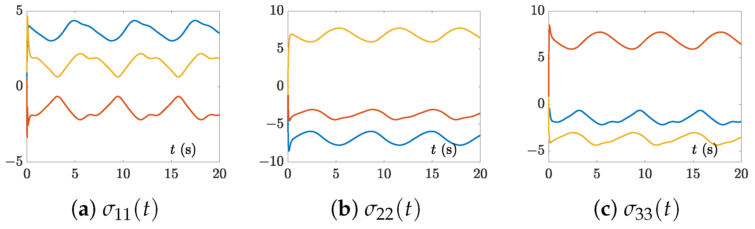
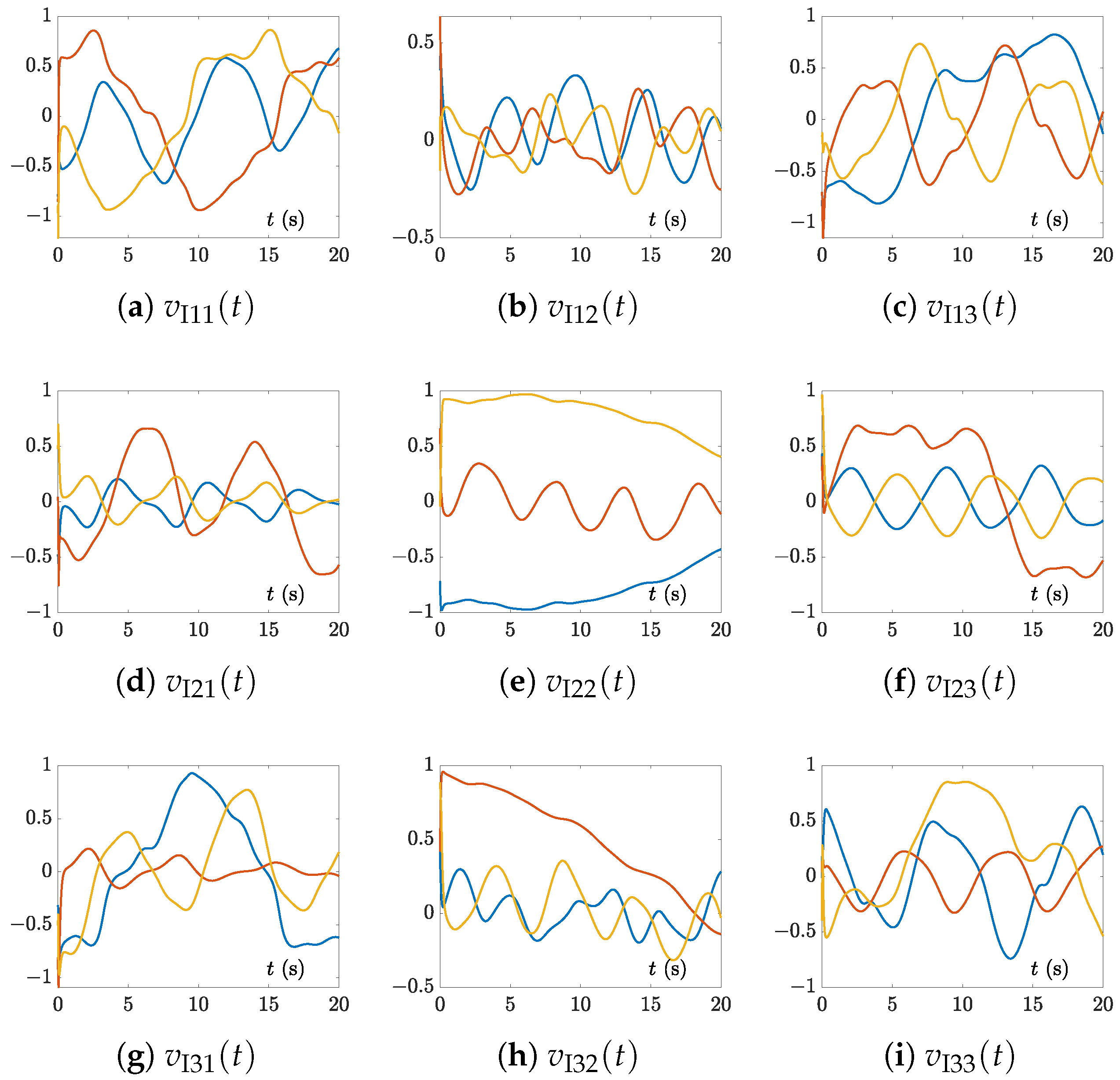
4.2. Experimental Results of the CTSVD Model

The ODE (ordinary differential equation) solver [31] in the MATLAB R2024a routine was first applied to execute the CTSVD model (7). Specifically, we used the ODE function “ode45” in this research, and the solving results are displayed in Figure 1, Figure 2, Figure 3, Figure 4, Figure 5, Figure 6, Figure 7, Figure 8 and Figure 9. Note that in Figure 1, Figure 2, Figure 3, Figure 4, Figure 5, Figure 6, Figure 7, Figure 8 and Figure 9, the solution trajectories and residual error trajectories corresponding to different initial values are represented in different colors.

Figure 1. Solution trajectories of $\Sigma \left(t\right)$ synthesized by the CTSVD model (7) with three random initial values and $\vartheta =10$ for Example 1.

Figure 2. Solution trajectories of $U_{\mathrm{R}}\left(t\right)$ synthesized by the CTSVD model (7) with three random initial values and $\vartheta =10$ for Example 1.

Figure 3. Solution trajectories of $U_{\mathrm{I}}\left(t\right)$ synthesized by the CTSVD model (7) with three random initial values and $\vartheta =10$ for Example 1.

Figure 4. Solution trajectories of $V_{\mathrm{R}}\left(t\right)$ synthesized by the CTSVD model (7) with three random initial values and $\vartheta =10$ for Example 1.

Figure 5. Solution trajectories of $V_{\mathrm{I}}\left(t\right)$ synthesized by the CTSVD model (7) with three random initial values and $\vartheta =10$ for Example 1.

Figure 6. Residual errors of the CTSVD model (7) with three random initial values and $\vartheta =10$ for Example 1.

Figure 7. Residual errors of the CTSVD model (7) with three random initial values and $\vartheta =10$ for Example 2.

Figure 8. Residual errors of the CTSVD model (7) with three random initial values and $\vartheta =10$ for Example 3.

Figure 9. Residual errors of the original problem (1), i.e., $\parallel C\left(t\right)-U\left(t\right)\Sigma \left(t\right)V^{*}{\left(t\right)\parallel }_{\mathrm{F}}$, corresponding to the CTSVD model (7) with three random initial values and $\vartheta =10$ for Examples 1–3.

The solution trajectories of $\Sigma \left(t\right)$ synthesized by the CTSVD model (7) with three random initial values and $\vartheta =10$ corresponding to Example 1 are shown in Figure 1. It is worth noting that $\Sigma \left(t\right)$ was a real-valued diagonal matrix, that is, its non-diagonal elements were zero, and the imaginary part of its diagonal elements were also zero. Therefore, in the three subgraphs (a), (b), and (c) of Figure 1, only the real part trajectories of the diagonal elements of $\Sigma \left(t\right)$, i.e., ${\sigma }_{11}\left(t\right)$, ${\sigma }_{22}\left(t\right)$, and ${\sigma }_{33}\left(t\right)$, are shown.

In addition, the solution trajectories of $U_{\mathrm{R}}\left(t\right)$, $U_{\mathrm{I}}\left(t\right)$, $V_{\mathrm{R}}\left(t\right)$, and $V_{\mathrm{I}}\left(t\right)$, synthesized by the CTSVD model (7) with three random initial values and $\vartheta =10$ corresponding to Example 1 are shown in Figure 2, Figure 3, Figure 4 and Figure 5. Evidently, from these figures, we can see that the real and imaginary values of all elements of matrices $U\left(t\right)$ and $V\left(t\right)$ changed over time, that is, they were temporally variant. Meanwhile, due to the page limitation and similarity, the solution trajectories synthesized by the CTSVD model (7) corresponding to Examples 2 and 3 are omitted.

From Figure 6, we see that the residual errors of the CTSVD model (7) corresponding to Example 1, with three random initial values and $\vartheta =10$, converged to near-zero within one second. Specifically, it can be seen from the subgraphs (a), (b), (c), (d), (e), and (f) in Figure 6 that the values of the residual errors of the CTSVD model (7), i.e., $\parallel W_1{\left(t\right)\parallel }_{\mathrm{F}}$, $\parallel W_2{\left(t\right)\parallel }_{\mathrm{F}}$, $\parallel W_3{\left(t\right)\parallel }_{\mathrm{F}}$, $\parallel W_4{\left(t\right)\parallel }_{\mathrm{F}}$, $\parallel W_5{\left(t\right)\parallel }_{\mathrm{F}}$, and $\parallel W_6{\left(t\right)\parallel }_{\mathrm{F}}$, converged rapidly to near-zero, which means that the values of the error functions, i.e., $W_1\left(t\right)$, $W_2\left(t\right)$, $W_3\left(t\right)$, $W_4\left(t\right)$, $W_5\left(t\right)$, and $W_6\left(t\right)$, quickly became near-zero. This indicates that the linear design formula successfully zeros out the error functions’ values, and this simultaneously verifies the correctness of the results of Theorem 1.

Similarly, as shown in Figure 7 and Figure 8, the residual errors of the CTSVD model (7) corresponding to Examples 2 and 3, with the same parameters as Example 1, also rapidly converged to near-zero. Moreover, as seen from Figure 9, the residual errors of original problem (1) for Examples 1–3 also converged to near-zero rapidly. Therefore, the results of Theorem 1 were confirmed to be correct again.

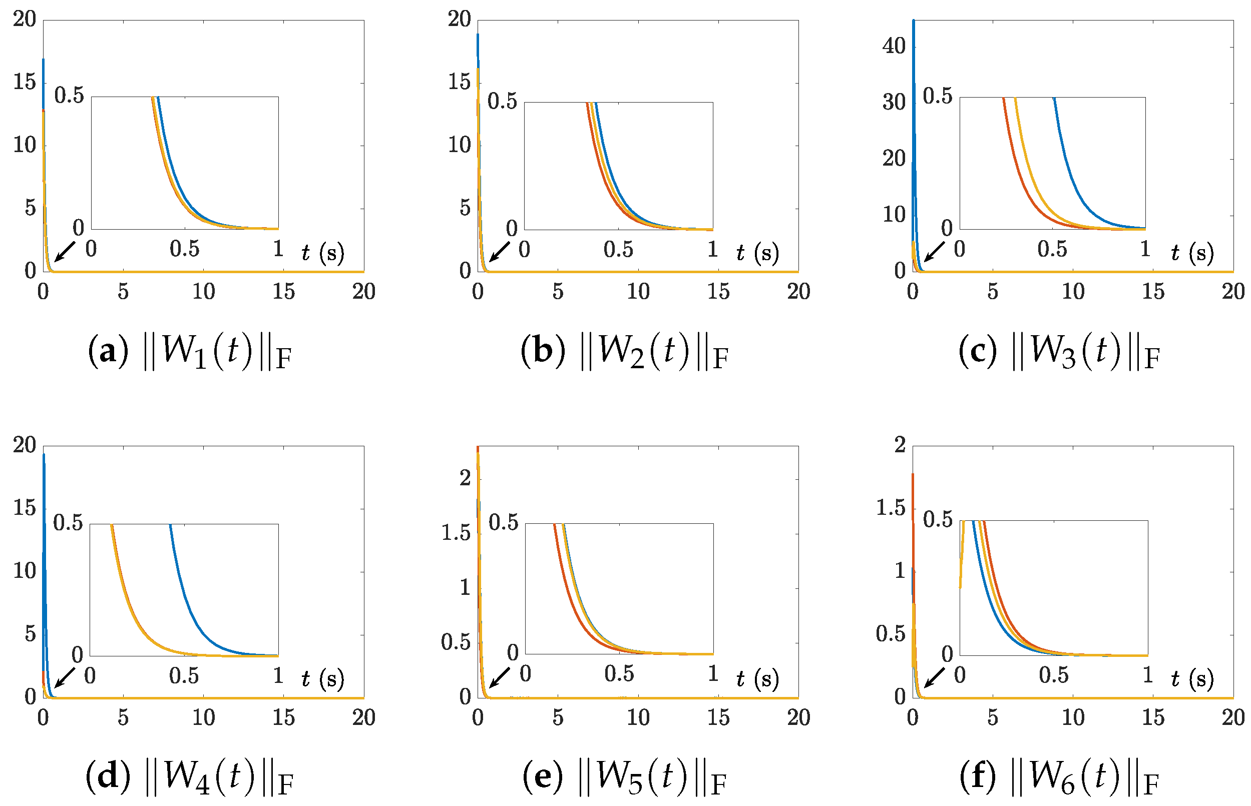
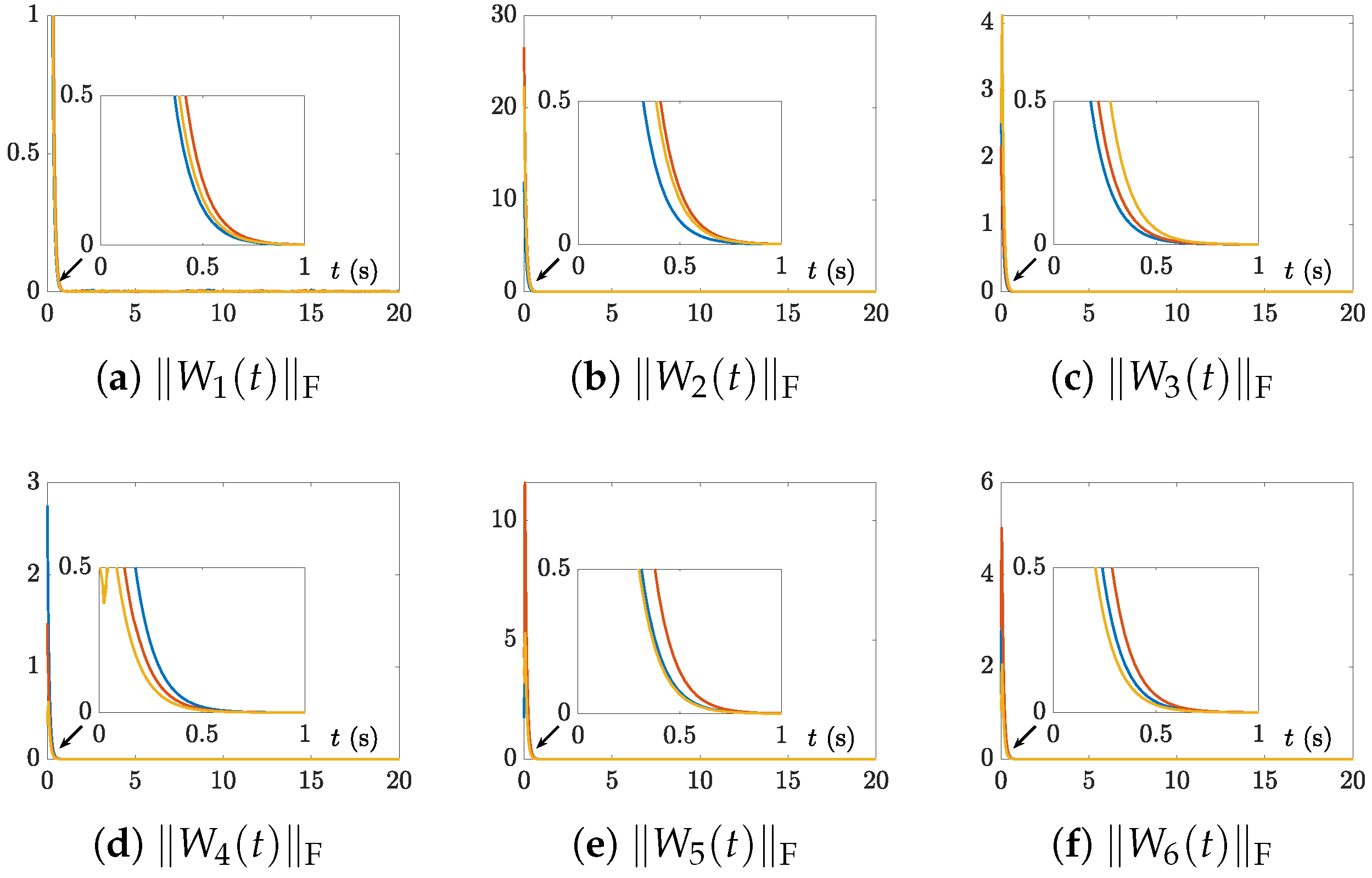
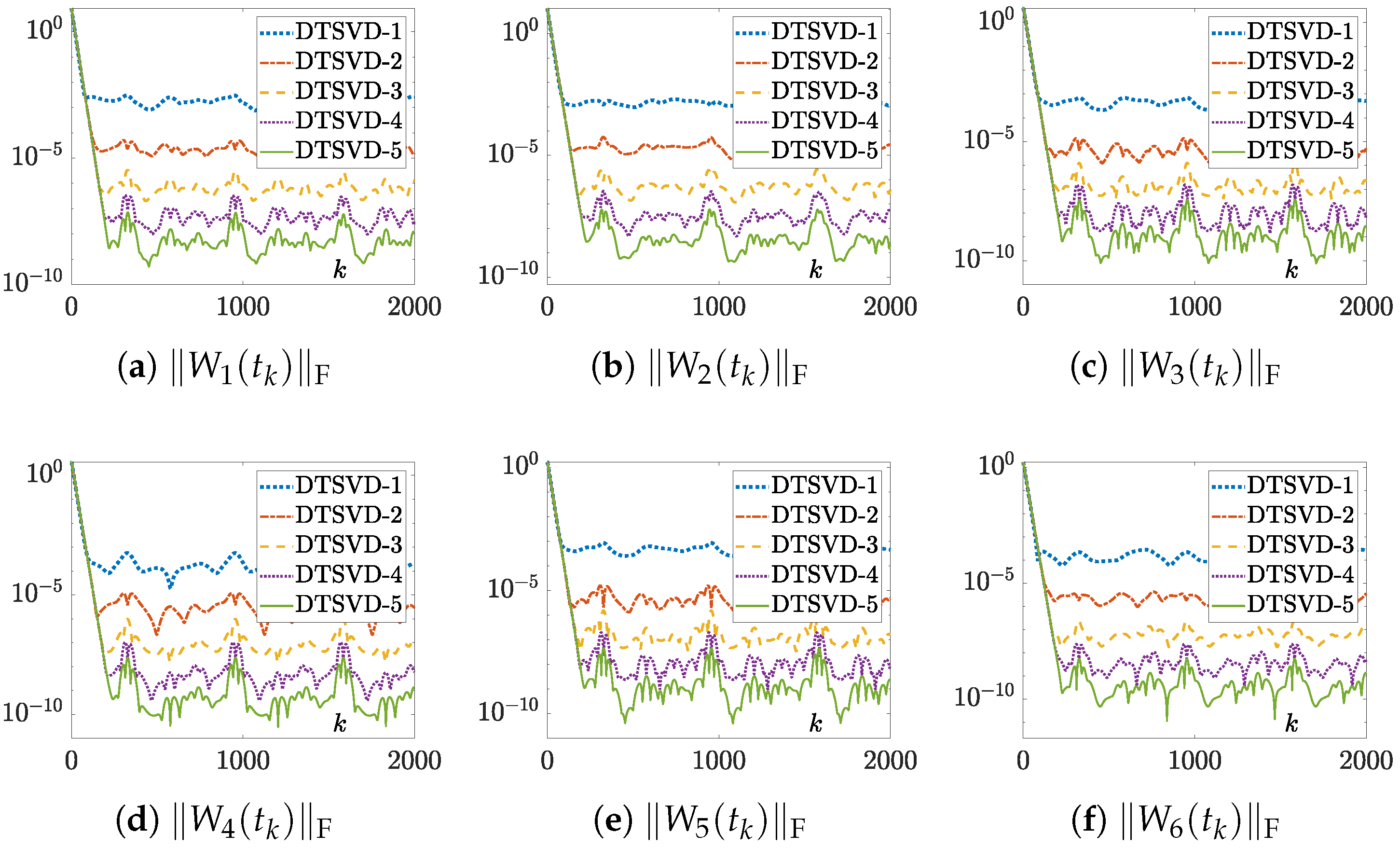
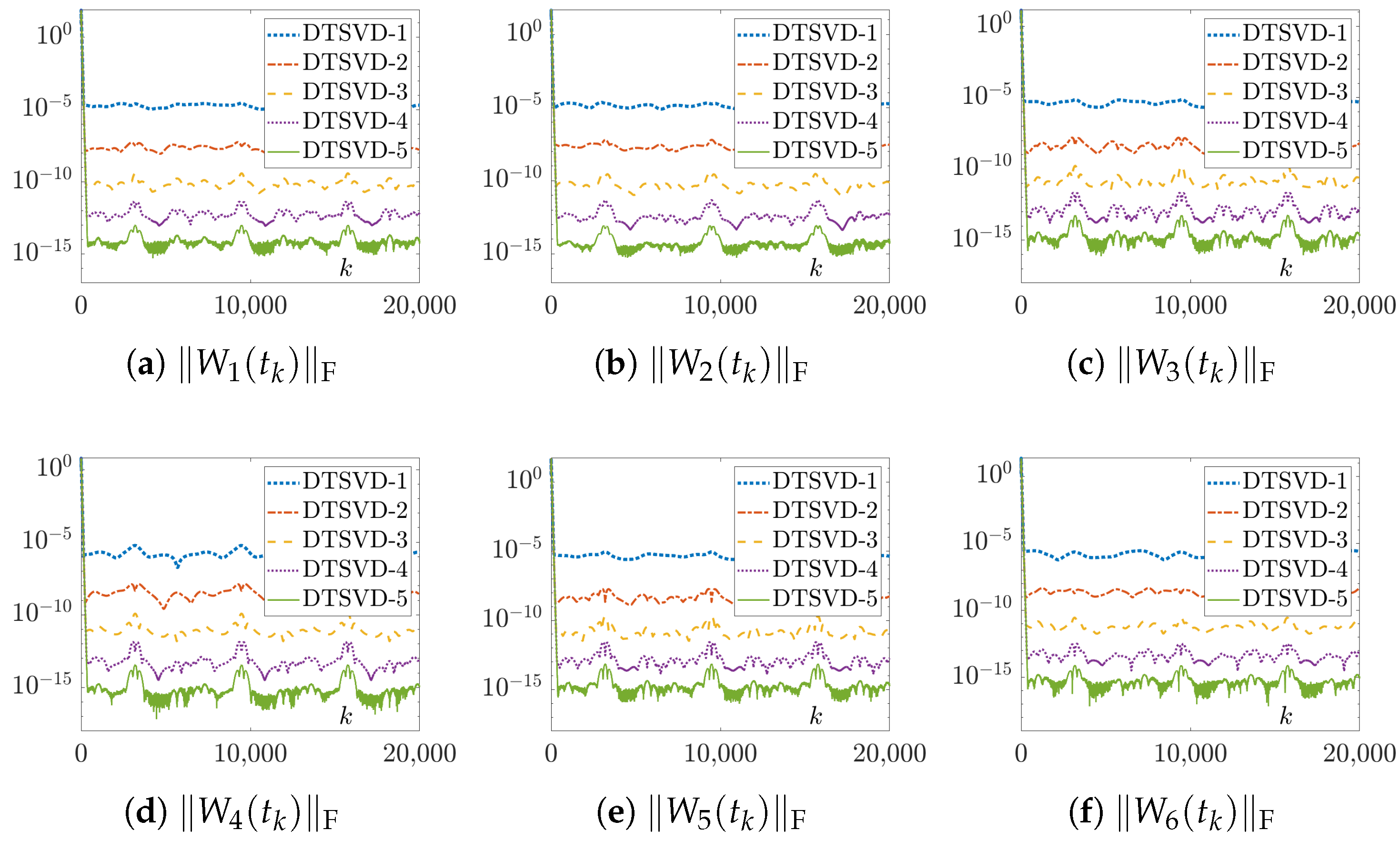
4.3. Experimental Results of DTSVD Algorithms

The results of the numerical experiments for the DTSVD-1 (24), -2 (25), -3 (26), -4 (27), and -5 (28) algorithms, with random initial values, $h=0.1$, and $\tau =0.001$ s or $0.0001$ s, are respectively displayed in Figure 10, Figure 11 and Figure 12, and the corresponding data are listed in Table 1, Table 2 and Table 3. Note that due to space limitations, the solution trajectory figures, as well as the residual error figures for Examples 2 and 3, synthesized by the DTSVD algorithms are not provided.

Figure 10. Residual errors of the DTSVD-1 (24), -2 (25), -3 (26), -4 (27), and -5 (28) algorithms with random initial values, $h=0.1$, and $\tau =0.01$ s for Example 1.

Figure 11. Residual errors of the DTSVD-1 (24), -2 (25), -3 (26), -4 (27), and -5 (28) algorithms with random initial values, $h=0.1$, and $\tau =0.001$ s for Example 1.

Figure 12. Residual errors of the original problem (1), i.e., $\parallel C\left(t_k\right)-U\left(t_k\right)\Sigma \left(t_k\right)V^{*}\left(t_k\right){\parallel }_{\mathrm{F}}$, corresponding to the DTSVD-1 (24), -2 (25), -3 (26), -4 (27), and -5 (28) algorithms with random initial values and $h=0.1$ for Examples 1–3. (a) Example 1 with $\tau =0.01$ s. (b) Example 2 with $\tau =0.01$ s. (c) Example 3 with $\tau =0.01$ s. (d) Example 1 with $\tau =0.001$ s. (e) Example 2 with $\tau =0.001$ s. (f) Example 3 with $\tau =0.001$ s.

Table 1. Residual errors of (24), (25), and (26), with $h=0.1$.

Algorithm		$\mathit{\tau }$ (s)	Example 1	Example 2	Example 3	Law
DTSVD-1 (24)	$\parallel W_1\left(t_k\right){\parallel }_{\mathrm{F}}$	$0.01$	$3.041\times$${10}^{-3}$	$3.183\times$${10}^{-3}$	$3.082\times$${10}^{-3}$	$O\left({\tau }^2\right)$
		$0.001$	$2.653\times$${10}^{-5}$	$3.405\times$${10}^{-5}$	$3.028\times$${10}^{-5}$
	$\parallel W_2\left(t_k\right){\parallel }_{\mathrm{F}}$	$0.01$	$1.791\times$${10}^{-3}$	$1.599\times$${10}^{-3}$	$1.888\times$${10}^{-3}$
		$0.001$	$2.252\times$${10}^{-5}$	$1.877\times$${10}^{-5}$	$1.915\times$${10}^{-5}$
	$\parallel W_3\left(t_k\right){\parallel }_{\mathrm{F}}$	$0.01$	$7.008\times$${10}^{-4}$	$1.145\times$${10}^{-3}$	$6.417\times$${10}^{-4}$
		$0.001$	$7.271\times$${10}^{-6}$	$1.158\times$${10}^{-5}$	$6.512\times$${10}^{-6}$
	$\parallel W_4\left(t_k\right){\parallel }_{\mathrm{F}}$	$0.01$	$5.660\times$${10}^{-4}$	$3.952\times$${10}^{-4}$	$3.291\times$${10}^{-4}$
		$0.001$	$5.911\times$${10}^{-6}$	$4.119\times$${10}^{-6}$	$3.357\times$${10}^{-6}$
	$\parallel W_5\left(t_k\right){\parallel }_{\mathrm{F}}$	$0.01$	$8.677\times$${10}^{-4}$	$6.405\times$${10}^{-4}$	$1.146\times$${10}^{-3}$
		$0.001$	$9.024\times$${10}^{-6}$	$6.546\times$${10}^{-6}$	$1.159\times$${10}^{-5}$
	$\parallel W_6\left(t_k\right){\parallel }_{\mathrm{F}}$	$0.01$	$2.216\times$${10}^{-4}$	$3.295\times$${10}^{-4}$	$3.936\times$${10}^{-4}$
		$0.001$	$2.250\times$${10}^{-6}$	$3.357\times$${10}^{-6}$	$4.120\times$${10}^{-6}$
DTSVD-2 (25)	$\parallel W_1\left(t_k\right){\parallel }_{\mathrm{F}}$	$0.01$	$5.127\times$${10}^{-5}$	$4.322\times$${10}^{-5}$	$4.300\times$${10}^{-5}$	$O\left({\tau }^3\right)$
		$0.001$	$5.306\times$${10}^{-8}$	$4.813\times$${10}^{-8}$	$4.556\times$${10}^{-8}$
	$\parallel W_2\left(t_k\right){\parallel }_{\mathrm{F}}$	$0.01$	$5.620\times$${10}^{-5}$	$3.735\times$${10}^{-5}$	$4.215\times$${10}^{-5}$
		$0.001$	$6.168\times$${10}^{-8}$	$4.071\times$${10}^{-8}$	$3.931\times$${10}^{-8}$
	$\parallel W_3\left(t_k\right){\parallel }_{\mathrm{F}}$	$0.01$	$1.360\times$${10}^{-5}$	$1.333\times$${10}^{-5}$	$7.166\times$${10}^{-6}$
		$0.001$	$1.564\times$${10}^{-8}$	$1.493\times$${10}^{-8}$	$9.021\times$${10}^{-9}$
	$\parallel W_4\left(t_k\right){\parallel }_{\mathrm{F}}$	$0.01$	$1.156\times$${10}^{-5}$	$1.044\times$${10}^{-5}$	$5.195\times$${10}^{-6}$
		$0.001$	$1.308\times$${10}^{-8}$	$1.152\times$${10}^{-8}$	$5.605\times$${10}^{-9}$
	$\parallel W_5\left(t_k\right){\parallel }_{\mathrm{F}}$	$0.01$	$1.582\times$${10}^{-5}$	$8.336\times$${10}^{-6}$	$1.329\times$${10}^{-5}$
		$0.001$	$1.823\times$${10}^{-8}$	$9.041\times$${10}^{-9}$	$1.506\times$${10}^{-8}$
	$|\parallel W_6\left(t_k\right){\parallel }_{\mathrm{F}}$	$0.01$	$3.671\times$${10}^{-6}$	$5.195\times$${10}^{-6}$	$1.044\times$${10}^{-5}$
		$0.001$	$3.420\times$${10}^{-9}$	$5.598\times$${10}^{-9}$	$1.153\times$${10}^{-8}$
DTSVD-3 (26)	$\parallel W_1\left(t_k\right){\parallel }_{\mathrm{F}}$	$0.01$	$3.360\times$${10}^{-6}$	$1.837\times$${10}^{-6}$	$1.827\times$${10}^{-6}$	$O\left({\tau }^4\right)$
		$0.001$	$3.782\times$${10}^{-10}$	$2.063\times$${10}^{-10}$	$1.983\times$${10}^{-10}$
	$\parallel W_2\left(t_k\right){\parallel }_{\mathrm{F}}$	$0.01$	$2.348\times$${10}^{-6}$	$1.284\times$${10}^{-6}$	$1.414\times$${10}^{-6}$
		$0.001$	$3.015\times$${10}^{-10}$	$1.526\times$${10}^{-10}$	$1.410\times$${10}^{-10}$
	$\parallel W_3\left(t_k\right){\parallel }_{\mathrm{F}}$	$0.01$	$1.257\times$${10}^{-6}$	$8.094\times$${10}^{-7}$	$4.141\times$${10}^{-7}$
		$0.001$	$1.643\times$${10}^{-10}$	$9.092\times$${10}^{-11}$	$4.606\times$${10}^{-11}$
	$\parallel W_4\left(t_k\right){\parallel }_{\mathrm{F}}$	$0.01$	$9.666\times$${10}^{-7}$	$4.619\times$${10}^{-7}$	$2.576\times$${10}^{-7}$
		$0.001$	$1.205\times$${10}^{-10}$	$5.549\times$${10}^{-11}$	$2.868\times$${10}^{-11}$
	$\parallel W_5\left(t_k\right){\parallel }_{\mathrm{F}}$	$0.01$	$1.532\times$${10}^{-6}$	$4.105\times$${10}^{-7}$	$8.087\times$${10}^{-7}$
		$0.001$	$2.014\times$${10}^{-10}$	$4.623\times$${10}^{-11}$	$9.104\times$${10}^{-11}$
	$\parallel W_6\left(t_k\right){\parallel }_{\mathrm{F}}$	$0.01$	$2.350\times$${10}^{-7}$	$2.576\times$${10}^{-7}$	$4.613\times$${10}^{-7}$
		$0.001$	$2.862\times$${10}^{-11}$	$2.854\times$${10}^{-11}$	$5.540\times$${10}^{-11}$

Table 2. Residual errors of (27) and (28), with $h=0.1$, in addition to Table 1.

Algorithm		$\mathit{\tau }$ (s)	Example 1	Example 2	Example 3	Law
DTSVD-4 (27)	$\parallel W_1\left(t_k\right){\parallel }_{\mathrm{F}}$	$0.01$	$3.404\times$${10}^{-7}$	$1.308\times$${10}^{-7}$	$1.295\times$${10}^{-7}$	$O\left({\tau }^5\right)$
		$0.001$	$4.090\times$${10}^{-12}$	$1.485\times$${10}^{-12}$	$1.461\times$${10}^{-12}$
	$\parallel W_2\left(t_k\right){\parallel }_{\mathrm{F}}$	$0.01$	$3.403\times$${10}^{-7}$	$1.033\times$${10}^{-7}$	$1.496\times$${10}^{-7}$
		$0.001$	$4.637\times$${10}^{-12}$	$1.349\times$${10}^{-12}$	$1.397\times$${10}^{-12}$
	$\parallel W_3\left(t_k\right){\parallel }_{\mathrm{F}}$	$0.01$	$1.541\times$${10}^{-7}$	$7.472\times$${10}^{-8}$	$2.744\times$${10}^{-8}$
		$0.001$	$2.076\times$${10}^{-12}$	$9.294\times$${10}^{-13}$	$3.490\times$${10}^{-13}$
	$\parallel W_4\left(t_k\right){\parallel }_{\mathrm{F}}$	$0.01$	$1.044\times$${10}^{-7}$	$5.119\times$${10}^{-8}$	$1.687\times$${10}^{-8}$
		$0.001$	$1.346\times$${10}^{-12}$	$6.408\times$${10}^{-13}$	$2.067\times$${10}^{-13}$
	$\parallel W_5\left(t_k\right){\parallel }_{\mathrm{F}}$	$0.01$	$1.987\times$${10}^{-7}$	$3.024\times$${10}^{-8}$	$7.492\times$${10}^{-8}$
		$0.001$	$2.449\times$${10}^{-12}$	$3.502\times$${10}^{-13}$	$9.293\times$${10}^{-13}$
	$\parallel W_6\left(t_k\right){\parallel }_{\mathrm{F}}$	$0.01$	$2.333\times$${10}^{-8}$	$1.763\times$${10}^{-8}$	$5.120\times$${10}^{-8}$
		$0.001$	$3.246\times$${10}^{-13}$	$2.120\times$${10}^{-13}$	$6.395\times$${10}^{-13}$
DTSVD-5 (28)	$\parallel W_1\left(t_k\right){\parallel }_{\mathrm{F}}$	$0.01$	$7.144\times$${10}^{-8}$	$1.858\times$${10}^{-8}$	$1.839\times$${10}^{-8}$	$O\left({\tau }^6\right)$
		$0.001$	$1.005\times$${10}^{-13}$	$2.576\times$${10}^{-14}$	$2.796\times$${10}^{-14}$
	$\parallel W_2\left(t_k\right){\parallel }_{\mathrm{F}}$	$0.01$	$5.873\times$${10}^{-8}$	$1.417\times$${10}^{-8}$	$1.859\times$${10}^{-8}$
		$0.001$	$8.367\times$${10}^{-14}$	$2.046\times$${10}^{-14}$	$1.882\times$${10}^{-14}$
	$\parallel W_3\left(t_k\right){\parallel }_{\mathrm{F}}$	$0.01$	$3.591\times$${10}^{-8}$	$9.548\times$${10}^{-9}$	$4.505\times$${10}^{-9}$
		$0.001$	$5.795\times$${10}^{-14}$	$1.235\times$${10}^{-14}$	$4.841\times$${10}^{-15}$
	$\parallel W_4\left(t_k\right){\parallel }_{\mathrm{F}}$	$0.01$	$2.356\times$${10}^{-8}$	$6.529\times$${10}^{-9}$	$2.694\times$${10}^{-9}$
		$0.001$	$3.619\times$${10}^{-14}$	$9.160\times$${10}^{-15}$	$3.370\times$${10}^{-15}$
	$\parallel W_5\left(t_k\right){\parallel }_{\mathrm{F}}$	$0.01$	$4.502\times$${10}^{-8}$	$4.568\times$${10}^{-9}$	$9.545\times$${10}^{-9}$
		$0.001$	$7.083\times$${10}^{-14}$	$5.772\times$${10}^{-15}$	$1.223\times$${10}^{-14}$
	$\parallel W_6\left(t_k\right){\parallel }_{\mathrm{F}}$	$0.01$	$5.364\times$${10}^{-9}$	$2.694\times$${10}^{-9}$	$6.528\times$${10}^{-9}$
		$0.001$	$7.938\times$${10}^{-15}$	$3.953\times$${10}^{-15}$	$8.195\times$${10}^{-15}$

Table 3. Residual errors of the original problem (1), i.e., $\parallel C\left(t_k\right)-U\left(t_k\right)\Sigma \left(t_k\right)V^{*}\left(t_k\right){\parallel }_{\mathrm{F}}$, for (24), (25), (26), (27), and (28), with $h=0.1$.

Algorithm	$\mathit{\tau }$ (s)	Example 1	Example 2	Example 3	Law
DTSVD-1 (24)	$0.01$	$2.369\times$${10}^{-3}$	$2.473\times$${10}^{-3}$	$2.473\times$${10}^{-3}$	$O\left({\tau }^2\right)$
	$0.001$	$2.401\times$${10}^{-5}$	$2.587\times$${10}^{-5}$	$2.588\times$${10}^{-5}$
DTSVD-2 (25)	$0.01$	$5.134\times$${10}^{-5}$	$3.024\times$${10}^{-5}$	$3.024\times$${10}^{-5}$	$O\left({\tau }^3\right)$
	$0.001$	$5.903\times$${10}^{-8}$	$3.253\times$${10}^{-8}$	$3.253\times$${10}^{-8}$
DTSVD-3 (26)	$0.01$	$2.111\times$${10}^{-6}$	$1.302\times$${10}^{-6}$	$1.302\times$${10}^{-6}$	$O\left({\tau }^4\right)$
	$0.001$	$2.557\times$${10}^{-10}$	$1.520\times$${10}^{-10}$	$1.521\times$${10}^{-10}$
DTSVD-4 (27)	$0.01$	$3.044\times$${10}^{-7}$	$1.086\times$${10}^{-7}$	$1.082\times$${10}^{-7}$	$O\left({\tau }^5\right)$
	$0.001$	$4.347\times$${10}^{-12}$	$1.287\times$${10}^{-12}$	$1.290\times$${10}^{-12}$
DTSVD-5 (28)	$0.01$	$5.075\times$${10}^{-8}$	$1.506\times$${10}^{-8}$	$1.506\times$${10}^{-8}$	$O\left({\tau }^6\right)$
	$0.001$	$7.519\times$${10}^{-14}$	$2.203\times$${10}^{-14}$	$2.225\times$${10}^{-14}$

By comparing Figure 10 and Figure 11, we can observe that the residual error trajectories synthesized by the DTSVD-1 (24), -2 (25), -3 (26), -4 (27), and -5 (28) algorithms for Example 1 changed regularly, which was consistent with the results of Theorem 3. From the subgraphs (a), (b), (c), (d), (e), and (f) in Figure 10 as well as Figure 11, we can observe that the values of the residual errors, i.e., $\parallel W_1\left(t_k\right){\parallel }_{\mathrm{F}}$, $\parallel W_2\left(t_k\right){\parallel }_{\mathrm{F}}$, $\parallel W_3\left(t_k\right){\parallel }_{\mathrm{F}}$, $\parallel W_4\left(t_k\right){\parallel }_{\mathrm{F}}$, $\parallel W_5\left(t_k\right){\parallel }_{\mathrm{F}}$, and $\parallel W_6\left(t_k\right){\parallel }_{\mathrm{F}}$, for the five DTSVD algorithms all converged rapidly to near-zero. Among these algorithms, the DTSVD-5 (28) algorithm had the fastest convergence speed and highest computational precision. In addition, as illustrated in Figure 10 and Figure 11, the values of the error functions, i.e., $W_1\left(t_k\right)$, $W_2\left(t_k\right)$, $W_3\left(t_k\right)$, $W_4\left(t_k\right)$, $W_5\left(t_k\right)$, and $W_6\left(t_k\right)$, rapidly approached zero, indicating the effectiveness of the proposed DTSVD algorithms.

Furthermore, according to the data in Table 1 and Table 2, we know that the residual errors of DTSVD-1 (24), -2 (25), -3 (26), -4 (27), and -5 (28) algorithms changed in the manner of $O\left({\tau }^2\right)$, $O\left({\tau }^3\right)$, $O\left({\tau }^4\right)$, $O\left({\tau }^5\right)$, and $O\left({\tau }^6\right)$, respectively, which verifies the results of Theorem 3. Meanwhile, as shown in Figure 12 and Table 3, the residual errors of the original problem (1) corresponding to the DTSVD-1 (24), -2 (25), -3 (26), -4 (27), and -5 (28) algorithms were also proportional to $O\left({\tau }^2\right)$, $O\left({\tau }^3\right)$, $O\left({\tau }^4\right)$, $O\left({\tau }^5\right)$, and $O\left({\tau }^6\right)$, respectively. Thus, Theorem 3’s results were reconfirmed.

5. Conclusions

In this research, the problem of complex, temporally variant SVD was formulated and investigated. To solve this difficult problem, an equation system was provided first. The dynamical model, i.e., the CTSVD model, was derived and proposed by applying the real ZN method, matrix vectorization, Kronecker product, vectorized transpose matrix, and dimensionality reduction technique. Meanwhile, a new 11-point ZeaD formula was proposed and studied. Furthermore, five DTSVD algorithms were obtained, with the use of the 11-point and other ZeaD formulas. It is worth mentioning that the proposed DTSVD-5 algorithm had the highest computational accuracy among the five DTSVD algorithms, i.e., $O\left({\tau }^6\right)$ precision. Finally, theoretical analyses and numerical experimental results verified the feasibility and effectiveness of the proposed dynamical model and algorithms. Our future research aims to apply the proposed SVD model and algorithms to real-world applications, such as signal processing, communications, and machine learning. Additionally, we will consider non-ideal conditions, including the existence of matrix singularities or noise interference.

References

- Ye, C.; Tan, S.; Wang, J.; Shi, L.; Zuo, Q.; Xiong, B. Double security level protection based on chaotic maps and SVD for medical images. Mathematics 2025, 13, 182. [Google Scholar] [CrossRef]
- Saifudin, I.; Widiyaningtyas, T.; Zaeni, I.; Aminuddin, A. SVD-GoRank: Recommender system algorithm using SVD and Gower’s ranking. IEEE Access 2025, 13, 19796–19827. [Google Scholar] [CrossRef]
- Tsyganov, A.; Tsyganova, Y. SVD-based parameter identification of discrete-time stochastic systems with unknown exogenous inputs. Mathematics 2024, 12, 1006. [Google Scholar] [CrossRef]
- Xie, Z.; Sun, J.; Tang, Y.; Tang, X.; Simpson, O.; Sun, Y. A k-SVD based compressive sensing method for visual chaotic image encryption. Mathematics 2023, 11, 1658. [Google Scholar] [CrossRef]
- Xue, Y.; Mu, K.; Wang, Y.; Chen, Y.; Zhong, P.; Wen, J. Robust speech steganography using differential SVD. IEEE Access 2019, 7, 153724–153733. [Google Scholar] [CrossRef]
- Wang, B.; Ding, C. An adaptive signal denoising method based on reweighted SVD for the fault diagnosis of rolling bearings. Sensors 2025, 25, 2470. [Google Scholar] [CrossRef]
- Baumann, M.; Helmke, U. Singular value decomposition of time-varying matrices. Future Gen. Comput. Syst. 2003, 19, 353–361. [Google Scholar] [CrossRef]
- Chen, J.; Zhang, Y. Online singular value decomposition of time-varying matrix via zeroing neural dynamics. Neurocomputing 2020, 383, 314–323. [Google Scholar] [CrossRef]
- Huang, M.; Zhang, Y. Zhang neuro-PID control for generalized bi-variable function projective synchronization of nonautonomous nonlinear systems with various perturbations. Mathematics 2024, 12, 2715. [Google Scholar] [CrossRef]
- Uhlig, F. Zhang neural networks: An introduction to predictive computations for discretized time-varying matrix problems. Numer. Math. 2024, 156, 691–739. [Google Scholar] [CrossRef]
- Guo, P.; Zhang, Y.; Li, S. Reciprocal-kind Zhang neurodynamics method for temporal-dependent Sylvester equation and robot manipulator motion planning. IEEE Trans. Neural Netw. Learn. Syst. 2025, 1–15. [Google Scholar] [CrossRef] [PubMed]
- Jerbi, H.; Alshammari, O.; Ben, A.; Kchaou, M.; Simos, T.; Mourtas, S.; Katsikis, V. Hermitian solutions of the quaternion algebraic Riccati equations through zeroing neural networks with application to quadrotor control. Mathematics 2024, 12, 15. [Google Scholar] [CrossRef]
- Jin, L.; Zhang, G.; Wang, Y.; Li, S. RNN-based quadratic programming scheme for tennis-training robots with flexible capabilities. IEEE Trans. Syst. Man Cybern. 2023, 53, 838–847. [Google Scholar] [CrossRef]
- Yang, Y.; Li, X.; Wang, X.; Liu, M.; Yin, J.; Li, W.; Voyles, R.; Ma, X. A strictly predefined-time convergent and anti-noise fractional-order zeroing neural network for solving time-variant quadratic programming in kinematic robot control. Neural Netw. 2025, 186, 107279. [Google Scholar] [CrossRef]
- Hua, C.; Cao, X.; Liao, B. Real-time solutions for dynamic complex matrix inversion and chaotic control using ODE-based neural computing methods. Comput. Intell. 2025, 41, e70042. [Google Scholar] [CrossRef]
- Zhang, B.; Zheng, Y.; Li, S.; Chen, X.; Mao, Y.; Pham, D. Inverse-free hybrid spatial-temporal derivative neural network for time-varying matrix Moore-Penrose inverse and its circuit schematic. IEEE Trans. Circuits-II 2025, 72, 499–503. [Google Scholar] [CrossRef]
- Yan, D.; Li, C.; Wu, J.; Deng, J.; Zhang, Z.; Yu, J.; Liu, P. A novel error-based adaptive feedback zeroing neural network for solving time-varying quadratic programming problems. Mathematics 2024, 12, 2090. [Google Scholar] [CrossRef]
- Peng, Z.; Huang, Y.; Xu, H. A novel high-efficiency variable parameter double integration ZNN model for time-varying Sylvester equations. Mathematics 2025, 13, 706. [Google Scholar] [CrossRef]
- Uhlig, F. Adapted AZNN methods for time-varying and static matrix problems. Electron. J. Linear Algebra 2023, 39, 164–180. [Google Scholar] [CrossRef]
- Guo, D.; Lin, X. Li-function activated Zhang neural network for online solution of time-varying linear matrix inequality. Neural Process. Lett. 2020, 52, 713–726. [Google Scholar] [CrossRef]
- Katsikis, V.N.; Mourtas, S.D.; Stanimirovic, P.S.; Zhang, Y. Solving complex-valued time-varying linear matrix equations via QR decomposition with applications to robotic motion tracking and on angle-of-arrival localization. IEEE Trans. Neural Netw. Learn. Syst. 2022, 33, 3415–3424. [Google Scholar] [CrossRef] [PubMed]
- Chen, J.; Kang, X.; Zhang, Y. Continuous and discrete ZND models with aid of eleven instants for complex QR decomposition of time-varying matrices. Mathematics 2023, 11, 3354. [Google Scholar] [CrossRef]
- Hu, C.; Kang, X.; Zhang, Y. Three-step general discrete-time Zhang neural network design and application to time-variant matrix inversion. Neurocomputing 2018, 306, 108–118. [Google Scholar] [CrossRef]
- Liu, K.; Liu, Y.; Zhang, Y.; Wei, L.; Sun, Z.; Jin, L. Five-step discrete-time noise-tolerant zeroing neural network model for time-varying matrix inversion with application to manipulator motion generation. Eng. Appl. Artif. Intel. 2021, 103, 104306. [Google Scholar] [CrossRef]
- Sun, M.; Wang, Y. General five-step discrete-time Zhang neural network for time-varying nonlinear optimization. Bull. Malays. Math. Sci. Soc. 2020, 43, 1741–1760. [Google Scholar] [CrossRef]
- Chen, J.; Zhang, Y. Discrete-time ZND models solving ALRMPC via eight-instant general and other formulas of ZeaD. IEEE Access 2019, 7, 125909–125918. [Google Scholar] [CrossRef]
- Brookes, M. The Matrix Reference Manual; Imperial College London Staff Page. 2020. Available online: http://www.ee.imperial.ac.uk/hp/staff/dmb/matrix/intro.html (accessed on 31 March 2025).
- Horn, R.A.; Johnson, C.R. Topics in Matrix Analysis; Cambridge University Press: New York, NY, USA, 1991. [Google Scholar]
- Zhang, Y.; Yang, R.; Li, S. Reciprocal Zhang dynamics (RZD) handling TVUDLMVE (time-varying under-determined linear matrix-vector equation). In Proceedings of the 37th Chinese Control and Decision Conference (CCDC), Xiamen, China, 16–19 May 2025; pp. 5794–5800. [Google Scholar]
- Griffiths, D.F.; Higham, D.J. Numerical Methods for Ordinary Differential Equations: Initial Value Problems; Springer: London, UK, 2010. [Google Scholar]
- Mathews, J.H.; Fink, K.D. Numerical Methods Using MATLAB; Prentice-Hall: Englewood Cliffs, NJ, USA, 2004. [Google Scholar]
- Suli, E.; Mayers, D.F. An Introduction to Numerical Analysis; Cambridge University Press: Oxford, UK, 2003. [Google Scholar]
Disclaimer/Publisher’s Note: The statements, opinions and data contained in all publications are solely those of the individual author(s) and contributor(s) and not of MDPI and/or the editor(s). MDPI and/or the editor(s) disclaim responsibility for any injury to people or property resulting from any ideas, methods, instructions or products referred to in the content. |
© 2025 by the authors. Licensee MDPI, Basel, Switzerland. This article is an open access article distributed under the terms and conditions of the Creative Commons Attribution (CC BY) license (https://creativecommons.org/licenses/by/4.0/).