Efficient 5-Point Block Method for Oscillatory ODEs with Phase Lag and Amplification Error Control

Abstract

This research presents innovative modified explicit block methods with fifth-order algebraic accuracy to address initial value problems (IVPs). The derivation of the methods employs fitting coefficients that eliminate phase lag and amplification error, as well as their derivatives. A thorough stability analysis of the new approach is conducted. Comparative assessments with existing methods highlight the superior effectiveness of the proposed algorithms. Numerical tests verify that this technique significantly surpasses conventional methods for solving IVPs, particularly those exhibiting oscillatory solutions.

1. Introduction

Differential equations with oscillatory solutions model systems exhibiting periodic or cyclic behavior, such as mechanical vibrations, electrical circuits, and biological rhythms. These equations often involve sinusoidal or other periodic functions, and accurately capturing their oscillations is crucial for understanding natural phenomena. Due to their repetitive nature, solving such equations typically requires specialized numerical methods, making this an important area of research [1]. Runge–Kutta and linear multi-step methods are well-known classes of methods that are widely used in approximating the solution of the initial value problems (IVPs). Other classes of methods for integrating IVP include hybrid methods, adapted Falkner-type methods, exponentially fitted methods, and trigonometrically fitted methods [2,3,4,5,6,7,8,9,10,11,12], etc. For a detailed survey of different classes of methods, one can consult the books by Butcher [13] and Hairer et al. [14] (and also references therein). These methods evaluate the numerical solution sequentially, at one point at a time. However, more efficient computational schemes can be devised by enabling the simultaneous calculation of solutions at multiple points. This approach is referred to as the block method. Block methods for the numerical solution of first-order ordinary differential equations (ODEs) have been developed by several researchers. Notable contributions include those by Birta et al. [15], Chu and Hamilton [16], Shampine and Watt [17], and Tam et al. [18]. From the literature, the following key observations motivate our work:

• Hybrid multi-step methods were implemented by Gragg and Stetter [19] to address stiff systems, while the block methods introduced by Milne [20], provide computational efficiency through parallel computing.
• To further address stiffness, hybrid block methods were developed, followed by optimized hybrid block methods [21] that combine the advantages of stability and block structuring. However, these methods primarily focus on reducing local truncation error and are not well-suited for handling highly oscillatory solutions.
• In problems involving high-frequency oscillations, recovering detailed information such as amplitude, energy, envelope, and especially phase becomes crucial. However, achieving this over long time intervals is challenging. Efficiency often requires a trade-off, accepting phase and amplification errors to allow for larger step sizes, as seen in real-time simulations.
• Many existing numerical methods assume a nearly linear problem structure, limiting their applicability. In contrast, block methods can effectively handle non-linear problems, making them suitable for a wide range of real-world applications.

Despite the extensive research in this field, there has been a notable gap in the development of block methods with minimal phase lag or amplification/phase-fitted block methods specifically designed for first-order IVPs. This work aims to introduce a numerical integrator designed to solve initial value problems of the form

$${\displaystyle \frac{dy}{dx}}=f(x,y),y\left(x_0\right)=y_0,$$

(1)

where $x\in [x_0,x_N]$, $y^{\prime }\left(x\right)$ represents the rate of change in the system, $f(x,y)$ is a function describing the system’s dynamics, and $y\left(x_0\right)=y_0$ provides the initial condition. We develop a zero-stable explicit block method and apply the theory for calculating phase lag and amplification error (or amplification factor) [9]. We also present methodologies for constructing amplification-fitted and phase-fitted block methods.

The paper is structured as follows: in Section 2, we derive explicit zero-stable five-points block method of order 5 and use the theory from [9] for calculating the phase lag and amplification error (or amplification factor) associated with block methods for solving first-order initial value problems (IVPs). Section 3 is dedicated to the development of methodologies aimed at optimizing the phase lag, amplification factor, and achieving phase-fitted and amplification-fitted block methods. Specifically, we present strategies for minimizing the phase lag, methods for obtaining amplification-fitted block techniques, and a comprehensive approach for deriving both phase-fitted and amplification-fitted block methods. Additionally, we eliminate the first-order derivatives of the amplification factor and phase lag. In Section 4, we conduct a thorough stability analysis of the family of newly proposed methods, assessing their performance under various conditions. Finally, in Section 5, we provide detailed numerical results to demonstrate the effectiveness and accuracy of the proposed approaches.

2. Explicit Five-Point Block Method

According to Fatunla [22], the s-point m-step block method for (1) is given by the matrix finite difference equation:

$$Y_n=\sum _{i=1}^m{A}_i{Y}_{n-i}+h\sum _{i=0}^m{B}_i{F}_{n-i},$$

(2)

where

$$Y_n=\left[\begin{array}{c}{y}_{ns}\\ y_{ns+1}\\ \dots \\ y_{ns+s-1}\end{array}\right]\mathrm{and}{F}_n=\left[\begin{array}{c}{f}_{ns}\\ f_{ns+1}\\ \dots \\ f_{ns+s-1}\end{array}\right],$$

where $n=0,1,2,\dots ,$ and $f_{ns}=f(x_0+h\left(ns\right),y_{ns}).$

The block scheme is explicit if the coefficient matrix $B_0$ is a null matrix. According to [23,24], supposing function $y\left(x\right)$ to be smooth enough, linear difference operator $L(y\left(x_{i+1}\right):k)$ corresponding to the multi-step method is

$$L(y\left(x_{i+1}\right):h)=y(x_i+h)-\sum _{j=1}^k{\alpha }_j{y}_{i+1-j}-\sum _{j=0}^k{\beta }_j{f}_{i+1-j},$$

Expanding Taylor’s series expansion about $x_i$ yields $L(y\left(x_{i+1}\right):h)=c_{0}y\left(x_i\right)+c_{1}h{y}^{\prime }\left(x_i\right)+c_2{h}^2{y}^2\left(x_i\right)+\dots +c_p{h}^p{y}^p\left(x_i\right)+c_{p+1}{h}^{(p+1)}{y}^{(p+1)}\left(x_i\right)+\dots$ The order of a linear multi-step method is p if $c_0=c_1=c_2=\dots =c_p=0$ and $c_{p+1}\ne 0$. Chollom et al. [25] extended this approach for the entire block, and this technique will be used to define the order of the block method of the type (2). The local truncation error for the block method (2) in matrix form after Taylor’s expansion:

$$L[y\left(x\right);h]=h^{0}y\left(x\right)C_0+h^1{y}^{\prime }\left(x\right)C_1+h^2{y}^{\prime \prime }\left(x\right)C_2+\dots +h^p{y}^{\left(p\right)}\left(x\right)C_p+\dots .$$

If $C_0=C_1=C_2=\dots =C_p=0$ and $C_{p+1}\ne 0$, then the order of the block method is p and $C_{p+1}$ is error constant.

For the explicit five-point block method ($s=5$), we have the matrix finite difference equation:

$$Y_{n+1}=A{Y}_n+hB{F}_n,$$

(3)

with the coefficient matrices specified as

$$A=\left[\begin{array}{ccccc}{a}_{11}& a_{12}& a_{13}& a_{14}& a_{15}\\ a_{21}& a_{22}& a_{23}& a_{24}& a_{25}\\ a_{31}& a_{32}& a_{33}& a_{34}& a_{35}\\ a_{41}& a_{42}& a_{43}& a_{44}& a_{45}\\ a_{51}& a_{52}& a_{53}& a_{54}& a_{55}\end{array}\right],B=\left[\begin{array}{ccccc}{b}_{11}& b_{12}& b_{13}& b_{14}& b_{15}\\ b_{21}& b_{22}& b_{23}& b_{24}& b_{25}\\ b_{31}& b_{32}& b_{33}& b_{34}& b_{35}\\ b_{41}& b_{42}& b_{43}& b_{44}& b_{45}\\ b_{51}& b_{52}& b_{53}& b_{54}& b_{55}\end{array}\right].$$

Zero-stability ensures that the numerical method does not cause errors to increase as the computation advances. Therefore, for a zero-stable one-step explicit block method $Y_{n+1}=A{Y}_n+hB{F}_n$ of (5th order), we require the following:

1.

Local truncation error of $O\left(h^6\right)$.

2.

All eigenvalues of A must have magnitudes less than or equal to 1, and eigenvalues with a magnitude of 1 must have multiplicity 1.

There are numerous cases where we can find A with the above condition, and one of them is

$$A=\left[\begin{array}{ccccc}\frac{1}{15}& \frac{2}{15}& \frac{1}{5}& \frac{4}{15}& \frac{1}{3}\\ \\ \frac{1}{15}& \frac{2}{15}& \frac{1}{5}& \frac{4}{15}& \frac{1}{3}\\ \\ \frac{1}{15}& \frac{2}{15}& \frac{1}{5}& \frac{4}{15}& \frac{1}{3}\\ \\ \frac{1}{15}& \frac{2}{15}& \frac{1}{5}& \frac{4}{15}& \frac{1}{3}\\ \\ \frac{1}{15}& \frac{2}{15}& \frac{1}{5}& \frac{4}{15}& \frac{1}{3}\\ \end{array}\right].$$

(4)

Now, by expanding $Y_{n+1}-A{Y}_n-hB{F}_n$, using the Taylor series, we equate the co-efficient of $y^{\prime }\left(x\right),y^{\prime \prime }\left(x\right),\dots ,y^v\left(x\right)$ equal to zero in each row of the matrix. This gives 25 equations with 25 unknowns, and solving it using MATHEMATICA, which gives the following matrix

$$B_1=\left[\begin{array}{ccccc}\frac{767}{2160}& -\frac{1681}{1080}& \frac{337}{90}& -\frac{3319}{1080}& \frac{1237}{432}\\ \\ \frac{647}{216}& -\frac{7781}{540}& \frac{1277}{45}& -\frac{2791}{108}& \frac{13189}{1080}\\ \\ \frac{26663}{2160}& -\frac{63193}{1080}& \frac{9811}{90}& -\frac{102271}{1080}& \frac{78161}{2160}\\ \\ \frac{39223}{1080}& -\frac{91277}{540}& \frac{13709}{45}& -\frac{137051}{540}& \frac{94177}{1080}\\ \\ \frac{188639}{2160}& -\frac{86429}{216}& \frac{12677}{18}& -\frac{613783}{1080}& \frac{395657}{2160}\\ \end{array}\right].$$

The block method

$$Y_{n+1}=A{Y}_n+h{B}_1{F}_n,$$

(5)

has local truncation error:

$$LTE=\left[\begin{array}{c}\frac{461y^{\left(6\right)}\left(x\right)h^6}{1440}+O\left(h^7\right)\\ \frac{2369y^{\left(6\right)}\left(x\right)h^6}{720}+O\left(h^7\right)\\ \frac{22477y^{\left(6\right)}\left(x\right)h^6}{1440}+O\left(h^7\right)\\ \frac{37369y^{\left(6\right)}\left(x\right)h^6}{720}+O\left(h^7\right)\\ \frac{200461y^{\left(6\right)}\left(x\right)h^6}{1440}+O\left(h^7\right)\end{array}\right].$$

Considering the following scalar test equation:

$$y^{\prime }\left(x\right)=i\omega y\left(x\right),$$

(6)

with the exact solution given as:

$$y\left(x\right)=\exp \left(i\omega x\right),$$

(7)

we extend the approach used to evaluate the amplification factor for a multi-step method at a single step in the theory presented in [9] to evaluate it for the explicit block method (3). After employing block method (3) on IVP (6), one obtains

$$\left[\begin{array}{c}{y}_{n+5}\\ y_{n+6}\\ y_{n+7}\\ y_{n+8}\\ y_{n+9}\end{array}\right]=A\left[\begin{array}{c}{y}_n\\ y_{n+1}\\ y_{n+2}\\ y_{n+3}\\ y_{n+4}\end{array}\right]+h\left(i\omega \right)B\left[\begin{array}{c}{y}_n\\ y_{n+1}\\ y_{n+2}\\ y_{n+3}\\ y_{n+4}\end{array}\right].$$

(8)

Now, considering the substitution $v=\omega h$, the characteristic equation for the system of difference Equations (8) is as follows:

$$\left[\begin{array}{c}{\lambda }^5\\ {\lambda }^6\\ {\lambda }^7\\ {\lambda }^8\\ {\lambda }^9\end{array}\right]-A\left[\begin{array}{c}1\\ {\lambda }^1\\ {\lambda }^2\\ {\lambda }^3\\ {\lambda }^4\end{array}\right]=ivB\left[\begin{array}{c}1\\ {\lambda }^1\\ {\lambda }^2\\ {\lambda }^3\\ {\lambda }^4\end{array}\right].$$

(9)

Taking ${\lambda }^n={\exp }^{ni\theta \left(v\right)}=cos\left(n\theta \left(v\right)\right)+isin\left(n\theta \left(v\right)\right),n=1,2,\dots$, one obtains

$$\left[\begin{array}{c}cos\left(5\theta \right(v\left)\right)+isin\left(5\theta \right(v\left)\right)\\ cos\left(6\theta \right(v\left)\right)+isin\left(6\theta \right(v\left)\right)\\ cos\left(7\theta \right(v\left)\right)+isin\left(7\theta \right(v\left)\right)\\ cos\left(8\theta \right(v\left)\right)+isin\left(8\theta \right(v\left)\right)\\ cos\left(9\theta \right(v\left)\right)+isin\left(9\theta \right(v\left)\right)\end{array}\right]=(A+ivB)\left[\begin{array}{c}1\\ cos\left(\theta \right(v\left)\right)+isin\left(\theta \right(v\left)\right)\\ cos\left(2\theta \right(v\left)\right)+isin\left(2\theta \right(v\left)\right)\\ cos\left(3\theta \right(v\left)\right)+isin\left(3\theta \right(v\left)\right)\\ cos\left(4\theta \right(v\left)\right)+isin\left(4\theta \right(v\left)\right)\end{array}\right].$$

(10)

Definition 1

(Order of phase lag). Given that the theoretical solution of the scalar test Equation (6) at $x=h$ is equal to $\exp \left(i\omega h\right)$, or equivalently, $\exp \left(iv\right)$, and the numerical solution of the scalar test Equation (6) for $x=h$ is equal to $\exp \left(i\theta \right(v\left)\right)$, the phase lag is defined as:

$$\mathsf{\Phi }=vs.-\theta \left(v\right).$$

(11)

If the quantity $\mathsf{\Phi }=\mathcal{O}\left(v^{q+1}\right)$ as $v\to 0$, then it is said that the order of the phase lag is q.

Lemma 1.

The following relations are valid:

$$\begin{array}{cc}\hfill cos\left(j\theta \right(v\left)\right)& =cos\left(jv\right)+c{j}^2{v}^{q+2}+\mathcal{O}\left(v^{q+4}\right),\hfill \\ \hfill sin\left(j\theta \right(v\left)\right)& =sin\left(jv\right)-cj{v}^{q+1}+\mathcal{O}\left(v^{q+3}\right).\hfill \end{array}$$

(12)

For the proof, see [9].

Theorem 1

(Direct Formula for the Amplification Factor of a Block Method). For a five-point explicit block method (3), the amplification factor $AF$ is given by

$$AF=-v^{q+1}C=F^{-1}.\left(\left(\begin{array}{c}sin\left(5v\right)\\ sin\left(6v\right)\\ sin\left(7v\right)\\ sin\left(8v\right)\\ sin\left(9v\right)\end{array}\right)-A.\left(\begin{array}{c}0\\ sin\left(v\right)\\ sin\left(2v\right)\\ sin\left(3v\right)\\ sin\left(4v\right)\end{array}\right)-vB.\left(\begin{array}{c}1\\ cos\left(v\right)\\ cos\left(2v\right)\\ cos\left(3v\right)\\ cos\left(4v\right)\end{array}\right)\right),$$

(13)

where $F=-\left[\begin{array}{ccccc}5& 0& 0& 0& 0\\ 0& 6& 0& 0& 0\\ 0& 0& 7& 0& 0\\ 0& 0& 0& 8& 0\\ 0& 0& 0& 0& 9\end{array}\right]+A\left[\begin{array}{ccccc}0& 0& 0& 0& 0\\ 0& 1& 0& 0& 0\\ 0& 0& 2& 0& 0\\ 0& 0& 0& 3& 0\\ 0& 0& 0& 0& 4\end{array}\right]-v^{2}B\left[\begin{array}{ccccc}0& 0& 0& 0& 0\\ 0& 1^2& 0& 0& 0\\ 0& 0& 2^2& 0& 0\\ 0& 0& 0& 3^2& 0\\ 0& 0& 0& 0& 4^2\end{array}\right]$ and $v=\omega h$

Proof. 

From the established Lemma 1, we substitute the obtained relation (12) directly into the characteristic Equation (10), and one obtains

$$\begin{array}{c}\hfill \left[\begin{array}{c}cos\left(5v\right)+c_1{\left(5\right)}^2{v}^{q+2}+i(sin\left(5v\right)-c_1\left(5\right)v^{q+1})\\ cos\left(6v\right)+c_2{\left(6\right)}^2{v}^{q+2}+i(sin\left(6v\right)-c_2\left(6\right)v^{q+1})\\ cos\left(7v\right)+c_3{\left(7\right)}^2{v}^{q+2}+i(sin\left(7v\right)-c_3\left(7\right)v^{q+1})\\ cos\left(8v\right)+c_4{\left(8\right)}^2{v}^{q+2}+i(sin\left(8v\right)-c_4\left(8\right)v^{q+1})\\ cos\left(9v\right)+c_5{\left(9\right)}^2{v}^{q+2}+i(sin\left(9v\right)-c_5\left(9\right)v^{q+1})\end{array}\right]\\ \hfill =(A+ivB)\left[\begin{array}{c}1\\ cos\left(v\right)+c_2{\left(1\right)}^2{v}^{q+2}+i(sin\left(v\right)-c_2\left(1\right)v^{q+1})\\ cos\left(2v\right)+c_3{\left(2\right)}^2{v}^{q+2}+i(sin\left(2v\right)-c_3\left(2\right)v^{q+1})\\ cos\left(3v\right)+c_4{\left(3\right)}^2{v}^{q+2}+i(sin\left(3v\right)-c_4\left(3\right)v^{q+1})\\ cos\left(4v\right)+c_5{\left(4\right)}^2{v}^{q+2}+i(sin\left(4v\right)-c_5\left(4\right)v^{q+1})\end{array}\right],\end{array}$$

$$\begin{array}{cc}\hfill & \left[\begin{array}{c}cos\left(5v\right)+c_1{\left(5\right)}^2{v}^{q+2}\\ cos\left(6v\right)+c_2{\left(6\right)}^2{v}^{q+2}\\ cos\left(7v\right)+c_3{\left(7\right)}^2{v}^{q+2}\\ cos\left(8v\right)+c_4{\left(8\right)}^2{v}^{q+2}\\ cos\left(9v\right)+c_5{\left(9\right)}^2{v}^{q+2}\end{array}\right]+i\left[\begin{array}{c}sin\left(5v\right)-c_1\left(5\right)v^{q+1}\\ sin\left(6v\right)-c_2\left(6\right)v^{q+1}\\ sin\left(7v\right)-c_3\left(7\right)v^{q+1}\\ sin\left(8v\right)-c_4\left(8\right)v^{q+1}\\ sin\left(9v\right)-c_5\left(9\right)v^{q+1}\end{array}\right]\hfill \\ \hfill & =\left(A\left[\begin{array}{c}1\\ cos\left(v\right)+c_2{\left(1\right)}^2{v}^{q+2}\\ cos\left(2v\right)+c_3{\left(2\right)}^2{v}^{q+2}\\ cos\left(3v\right)+c_4{\left(3\right)}^2{v}^{q+2}\\ cos\left(4v\right)+c_5{\left(4\right)}^2{v}^{q+2}\end{array}\right]-vB\left[\begin{array}{c}0\\ sin\left(v\right)-c_2\left(1\right)v^{q+1}\\ sin\left(2v\right)-c_3\left(2\right)v^{q+1}\\ sin\left(3v\right)-c_4\left(3\right)v^{q+1}\\ sin\left(4v\right)-c_5\left(4\right)v^{q+1}\end{array}\right]\right)\hfill \\ \hfill & +i\left(A\left[\begin{array}{c}0\\ sin\left(v\right)-c_2\left(1\right)v^{q+1}\\ sin\left(2v\right)-c_3\left(2\right)v^{q+1}\\ sin\left(3v\right)-c_4\left(3\right)v^{q+1}\\ sin\left(4v\right)-c_5\left(4\right)v^{q+1}\end{array}\right]+vB\left[\begin{array}{c}1\\ cos\left(v\right)+c_2{\left(1\right)}^2{v}^{q+2}\\ cos\left(2v\right)+c_3{\left(2\right)}^2{v}^{q+2}\\ cos\left(3v\right)+c_4{\left(3\right)}^2{v}^{q+2}\\ cos\left(4v\right)+c_5{\left(4\right)}^2{v}^{q+2}\end{array}\right]\right).\hfill \end{array}$$

(14)

Now, the imaginary part of the above system is as follows

$$\begin{array}{c}\hfill \left[\begin{array}{c}sin\left(5v\right)-c_1\left(5\right)v^{q+1}\\ sin\left(6v\right)-c_2\left(6\right)v^{q+1}\\ sin\left(7v\right)-c_3\left(7\right)v^{q+1}\\ sin\left(8v\right)-c_4\left(8\right)v^{q+1}\\ sin\left(9v\right)-c_5\left(9\right)v^{q+1}\end{array}\right]=A\left[\begin{array}{c}0\\ sin\left(v\right)-c_2\left(1\right)v^{q+1}\\ sin\left(2v\right)-c_3\left(2\right)v^{q+1}\\ sin\left(3v\right)-c_4\left(3\right)v^{q+1}\\ sin\left(4v\right)-c_5\left(4\right)v^{q+1}\end{array}\right]+vB\left[\begin{array}{c}1\\ cos\left(v\right)+c_2{\left(1\right)}^2{v}^{q+2}\\ cos\left(2v\right)+c_3{\left(2\right)}^2{v}^{q+2}\\ cos\left(3v\right)+c_4{\left(3\right)}^2{v}^{q+2}\\ cos\left(4v\right)+c_5{\left(4\right)}^2{v}^{q+2}\end{array}\right],\end{array}$$

(15)

and further simplifying,

$$\begin{array}{cc}\hfill & -v^{q+1}\left(\left[\begin{array}{ccccc}5& 0& 0& 0& 0\\ 0& 6& 0& 0& 0\\ 0& 0& 7& 0& 0\\ 0& 0& 0& 8& 0\\ 0& 0& 0& 0& 9\end{array}\right]-A\left[\begin{array}{ccccc}0& 0& 0& 0& 0\\ 0& 1& 0& 0& 0\\ 0& 0& 2& 0& 0\\ 0& 0& 0& 3& 0\\ 0& 0& 0& 0& 4\end{array}\right]+v^{2}B\left[\begin{array}{ccccc}0& 0& 0& 0& 0\\ 0& 1^2& 0& 0& 0\\ 0& 0& 2^2& 0& 0\\ 0& 0& 0& 3^2& 0\\ 0& 0& 0& 0& 4^2\end{array}\right]\right)C\hfill \\ \hfill & =-\left[\begin{array}{c}sin\left(5v\right)\\ sin\left(6v\right)\\ sin\left(7v\right)\\ sin\left(8v\right)\\ sin\left(9v\right)\end{array}\right]+A\left[\begin{array}{c}0\\ sin\left(v\right)\\ sin\left(2v\right)\\ sin\left(3v\right)\\ sin\left(4v\right)\end{array}\right]+vB\left[\begin{array}{c}1\\ cos\left(v\right)\\ cos\left(2v\right)\\ cos\left(3v\right)\\ cos\left(4v\right)\end{array}\right],\hfill \end{array}$$

(16)

where $C={[c_1,c_2,c_3,c_4,c_5]}^T$. The direct formula for the computation of the amplification factor ($AF$) of the block method (3) is

$$-v^{q+1}C=F^{-1}.\left(\left(\begin{array}{c}sin\left(5v\right)\\ sin\left(6v\right)\\ sin\left(7v\right)\\ sin\left(8v\right)\\ sin\left(9v\right)\end{array}\right)-A.\left(\begin{array}{c}0\\ sin\left(v\right)\\ sin\left(2v\right)\\ sin\left(3v\right)\\ sin\left(4v\right)\end{array}\right)-vB.\left(\begin{array}{c}1\\ cos\left(v\right)\\ cos\left(2v\right)\\ cos\left(3v\right)\\ cos\left(4v\right)\end{array}\right)\right),$$

(17)

where $F=\left(-\left[\begin{array}{ccccc}5& 0& 0& 0& 0\\ 0& 6& 0& 0& 0\\ 0& 0& 7& 0& 0\\ 0& 0& 0& 8& 0\\ 0& 0& 0& 0& 9\end{array}\right]+A\left[\begin{array}{ccccc}0& 0& 0& 0& 0\\ 0& 1& 0& 0& 0\\ 0& 0& 2& 0& 0\\ 0& 0& 0& 3& 0\\ 0& 0& 0& 0& 4\end{array}\right]-v^{2}B\left[\begin{array}{ccccc}0& 0& 0& 0& 0\\ 0& 1^2& 0& 0& 0\\ 0& 0& 2^2& 0& 0\\ 0& 0& 0& 3^2& 0\\ 0& 0& 0& 0& 4^2\end{array}\right]\right)$.

□

Theorem 2

(Direct Formula for the Phase Lag of a Block Method). For a five-point block method, the phase lag $PhEr$ is expressed as

$$PhEr=-v^{q+2}C=E^{-1}.\left(\left(\begin{array}{c}cos\left(5v\right)\\ cos\left(6v\right)\\ cos\left(7v\right)\\ cos\left(8v\right)\\ cos\left(9v\right)\end{array}\right)-A.\left(\begin{array}{c}1\\ cos\left(v\right)\\ cos\left(2v\right)\\ cos\left(3v\right)\\ cos\left(4v\right)\end{array}\right)+vB.\left(\begin{array}{c}0\\ sin\left(v\right)\\ sin\left(2v\right)\\ sin\left(3v\right)\\ sin\left(4v\right)\end{array}\right)\right),$$

(18)

where $E=\left(\left[\begin{array}{ccccc}{5}^2& 0& 0& 0& 0\\ 0& 6^2& 0& 0& 0\\ 0& 0& 7^2& 0& 0\\ 0& 0& 0& 8^2& 0\\ 0& 0& 0& 0& 9^2\end{array}\right]-A\left[\begin{array}{ccccc}0& 0& 0& 0& 0\\ 0& 1^2& 0& 0& 0\\ 0& 0& 2^2& 0& 0\\ 0& 0& 0& 3^2& 0\\ 0& 0& 0& 0& 4^2\end{array}\right]-B\left[\begin{array}{ccccc}0& 0& 0& 0& 0\\ 0& 1& 0& 0& 0\\ 0& 0& 2& 0& 0\\ 0& 0& 0& 3& 0\\ 0& 0& 0& 0& 4\end{array}\right]\right)$ and $v=\omega h$.

Proof. 

Similar to the proof of Theorem 1, by applying the established Lemma 1, substitute the derived relation (12) into the characteristic Equation (9), leading to (15). Likewise, by comparing the real part of (15), one obtains

$$\begin{array}{c}\hfill \left[\begin{array}{c}cos\left(5v\right)+c_1{\left(5\right)}^2{v}^{q+2}\\ cos\left(6v\right)+c_2{\left(6\right)}^2{v}^{q+2}\\ cos\left(7v\right)+c_3{\left(7\right)}^2{v}^{q+2}\\ cos\left(8v\right)+c_4{\left(8\right)}^2{v}^{q+2}\\ cos\left(9v\right)+c_5{\left(9\right)}^2{v}^{q+2}\end{array}\right]=\left(A\left[\begin{array}{c}1\\ cos\left(v\right)+c_2{\left(1\right)}^2{v}^{q+2}\\ cos\left(2v\right)+c_3{\left(2\right)}^2{v}^{q+2}\\ cos\left(3v\right)+c_4{\left(3\right)}^2{v}^{q+2}\\ cos\left(4v\right)+c_5{\left(4\right)}^2{v}^{q+2}\end{array}\right]-vB\left[\begin{array}{c}0\\ sin\left(v\right)-c_2\left(1\right)v^{q+1}\\ sin\left(2v\right)-c_3\left(2\right)v^{q+1}\\ sin\left(3v\right)-c_4\left(3\right)v^{q+1}\\ sin\left(4v\right)-c_5\left(4\right)v^{q+1}\end{array}\right]\right).\end{array}$$

(19)

$$\begin{array}{cc}\hfill & -v^{q+2}\left(\left[\begin{array}{ccccc}{5}^2& 0& 0& 0& 0\\ 0& 6^2& 0& 0& 0\\ 0& 0& 7^2& 0& 0\\ 0& 0& 0& 8^2& 0\\ 0& 0& 0& 0& 9^2\end{array}\right]-A\left[\begin{array}{ccccc}0& 0& 0& 0& 0\\ 0& 1^2& 0& 0& 0\\ 0& 0& 2^2& 0& 0\\ 0& 0& 0& 3^2& 0\\ 0& 0& 0& 0& 4^2\end{array}\right]-B\left[\begin{array}{ccccc}0& 0& 0& 0& 0\\ 0& 1& 0& 0& 0\\ 0& 0& 2& 0& 0\\ 0& 0& 0& 3& 0\\ 0& 0& 0& 0& 4\end{array}\right]\right)C\hfill \\ \hfill & =\left[\begin{array}{c}cos\left(5v\right)\\ cos\left(6v\right)\\ cos\left(7v\right)\\ cos\left(8v\right)\\ cos\left(9v\right)\end{array}\right]-A\left[\begin{array}{c}1\\ cos\left(v\right)\\ cos\left(2v\right)\\ cos\left(3v\right)\\ cos\left(4v\right)\end{array}\right]+vB\left[\begin{array}{c}0\\ sin\left(v\right)\\ sin\left(2v\right)\\ sin\left(3v\right)\\ sin\left(4v\right)\end{array}\right],\hfill \end{array}$$

(20)

$$\begin{array}{cc}\hfill & -v^{q+2}C=E^{-1}\left(\left[\begin{array}{c}cos\left(5v\right)\\ cos\left(6v\right)\\ cos\left(7v\right)\\ cos\left(8v\right)\\ cos\left(9v\right)\end{array}\right]-A\left[\begin{array}{c}1\\ cos\left(v\right)\\ cos\left(2v\right)\\ cos\left(3v\right)\\ cos\left(4v\right)\end{array}\right]+vB\left[\begin{array}{c}0\\ sin\left(v\right)\\ sin\left(2v\right)\\ sin\left(3v\right)\\ sin\left(4v\right)\end{array}\right]\right),\hfill \\ \hfill \end{array}$$

(21)

where $E=\left[\begin{array}{ccccc}{5}^2& 0& 0& 0& 0\\ 0& 6^2& 0& 0& 0\\ 0& 0& 7^2& 0& 0\\ 0& 0& 0& 8^2& 0\\ 0& 0& 0& 0& 9^2\end{array}\right]-A\left[\begin{array}{ccccc}0& 0& 0& 0& 0\\ 0& 1^2& 0& 0& 0\\ 0& 0& 2^2& 0& 0\\ 0& 0& 0& 3^2& 0\\ 0& 0& 0& 0& 4^2\end{array}\right]-B\left[\begin{array}{ccccc}0& 0& 0& 0& 0\\ 0& 1& 0& 0& 0\\ 0& 0& 2& 0& 0\\ 0& 0& 0& 3& 0\\ 0& 0& 0& 0& 4\end{array}\right]$.

By expanding the formula (13) from Theorem 1 for method (5) with $B=B_1$, and using Taylor’s series expansion,

$$AF=\left[\begin{array}{c}\frac{25523v^7}{75600}-\frac{2507699v^9}{504000}+O\left(v^{10}\right)\\ \frac{967153v^7}{378000}-\frac{91852907v^9}{1800000}+O\left(v^{10}\right)\\ \frac{9664241v^7}{982800}-\frac{21462883901v^9}{85176000}+O\left(v^{10}\right)\\ \frac{16890553v^7}{604800}-\frac{7184693431v^9}{8064000}+O\left(v^{10}\right)\\ \frac{95054741v^7}{1436400}-\frac{467424875311v^9}{181944000}+O\left(v^{10}\right)\end{array}\right].$$

Thus, $q=6$ and the block method (5) is of the sixth-order amplification factor. Similarly, the phase error for (5) using Taylor’s expansion on direct formula (18) from Theorem 2 for (5) with $B=B_1$ is

$$PhEr=\left[\begin{array}{c}-\frac{461v^6}{11760}+\frac{5459v^8}{43200}+O\left(v^{10}\right)\\ -\frac{2369v^6}{9840}+\frac{10766521v^8}{12398400}+O\left(v^{10}\right)\\ -\frac{22477v^6}{29040}+\frac{114473717v^8}{36590400}+O\left(v^{10}\right)\\ -\frac{37369v^6}{19920}+\frac{212710921v^8}{25099200}+O\left(v^{10}\right)\\ -\frac{200461v^6}{52080}+\frac{181538531v^8}{9374400}+O\left(v^{10}\right)\end{array}\right].$$

Thus, $q=4$ and the block method (5) referred as $M1$ is of the fourth-order phase lag. □

2.1. Method 2: Amplification Fitted Block Method with Minimal Phase Lag

Using matrix A from (4) and the direct formula in (13), the following algorithm derives the amplification-fitted block method with minimal phase lag. Algorithm:

1.

Eliminate the amplification factor.

2.

Calculate the phase lag using the coefficient obtained in the previous step.

3.

Perform a Taylor series expansion on the computed phase lag.

4.

Solve the system of equations required to minimize the phase lag.

5.

Determine the remaining unknown coefficients by minimizing the local truncation error using the updated coefficients.

In accordance with the algorithm, elimination of amplification factor $AF$ of block method (3), where A is considered as (4) leads to following set of equations

$$\begin{array}{cc}\hfill b_5& =-b_{1}sec\left(4v\right)-b_{2}cos\left(v\right)sec\left(4v\right)-b_{3}cos\left(2v\right)sec\left(4v\right)-b_{4}cos\left(3v\right)sec\left(4v\right)\hfill \\ \hfill & -{\displaystyle \frac{(2sin(v)+3sin(2v)+4sin(3v)+5sin(4v)-15sin(5v\left)\right)sec\left(4v\right)}{15v}},\hfill \\ \hfill b_{10}& =-b_{6}sec\left(4v\right)-b_{7}cos\left(v\right)sec\left(4v\right)-b_{8}cos\left(2v\right)sec\left(4v\right)-b_{9}cos\left(3v\right)sec\left(4v\right)\hfill \\ \hfill & -{\displaystyle \frac{(2sin(v)+3sin(2v)+4sin(3v)+5sin(4v)-15sin(6v\left)\right)sec\left(4v\right)}{15v}},\hfill \\ \\ \hfill b_{15}& =-b_{11}sec\left(4v\right)-b_{12}cos\left(v\right)sec\left(4v\right)-b_{13}cos\left(2v\right)sec\left(4v\right)-b_{14}cos\left(3v\right)sec\left(4v\right)\hfill \\ \hfill & -{\displaystyle \frac{(2sin(v)+3sin(2v)+4sin(3v)+5sin(4v)-15sin(7v\left)\right)sec\left(4v\right)}{15v}},\hfill \\ \hfill b_{20}& =-b_{16}sec\left(4v\right)-b_{17}cos\left(v\right)sec\left(4v\right)-b_{18}cos\left(2v\right)sec\left(4v\right)-b_{19}cos\left(3v\right)sec\left(4v\right)\hfill \\ \hfill & -{\displaystyle \frac{(2sin(v)+3sin(2v)+4sin(3v)+5sin(4v)-15sin(8v\left)\right)sec\left(4v\right)}{15v}},\hfill \\ \\ \hfill b_{25}& =-b_{21}sec\left(4v\right)-b_{22}cos\left(v\right)sec\left(4v\right)-b_{23}cos\left(2v\right)sec\left(4v\right)-b_{24}cos\left(3v\right)sec\left(4v\right)\hfill \\ \hfill & -{\displaystyle \frac{(2sin(v)+3sin(2v)+4sin(3v)+5sin(4v)-15sin(9v\left)\right)sec\left(4v\right)}{15v}}.\hfill \end{array}$$

(22)

Further, the phase lag is evaluated by utilizing the above coefficient values, and then minimized by vanishing the coefficients of $v^2$, $v^4$, and $v^6$, which gives the following

$$b_4=-4b_1-3b_2-2b_3+{\displaystyle \frac{7}{6}},b_9=-4b_6-3b_7-2b_8-{\displaystyle \frac{1}{3}},b_{14}=-4b_{11}-3b_{12}-2b_{13}-{\displaystyle \frac{17}{6}},$$

$$b_{19}=-4b_{16}-3b_{17}-2b_{18}-{\displaystyle \frac{19}{3}},b_{24}=-4b_{21}-3b_{22}-2b_{23}-{\displaystyle \frac{65}{6}},b_3=-10b_1-4b_2+{\displaystyle \frac{77}{72}},$$

$$b_8=-10b_6-4b_7+{\displaystyle \frac{25}{36}},b_{13}=-10b_{11}-4b_{12}-{\displaystyle \frac{115}{72}},b_{18}=-10b_{16}-4b_{17}-{\displaystyle \frac{299}{36}},$$

$$b_{23}=-10b_{21}-4b_{22}-{\displaystyle \frac{1651}{72}},b_2={\displaystyle \frac{1097}{4320}}-6b_1,b_7={\displaystyle \frac{589}{2160}}-6b_6,$$

$$b_{12}=-6b_{11}-{\displaystyle \frac{247}{4320}},b_{17}=-6b_{16}-{\displaystyle \frac{6539}{2160}},b_{22}=-6b_{21}-{\displaystyle \frac{13259}{864}}.$$

The above set of equations produces the following local truncation error:

$LTE=\left[\begin{array}{c}\left(-2b_1{y}^{\prime }\left(x\right)w^2+\frac{337}{864}{y}^{\prime }\left(x\right)w^2-2b_1{y}^{\left(3\right)}\left(x\right)+\frac{337}{864}{y}^{\left(3\right)}\left(x\right)\right)h^3+O\left(h^5\right)\\ \\ \left(-2b_6{y}^{\prime }\left(x\right)w^2+\frac{5833}{2160}{y}^{\prime }\left(x\right)w^2-2b_6{y}^{\left(3\right)}\left(x\right)+\frac{5833}{2160}{y}^{\left(3\right)}\left(x\right)\right)h^3+O\left(h^5\right)\\ \\ \left(-2b_{11}{y}^{\prime }\left(x\right)w^2+\frac{39221}{4320}{y}^{\prime }\left(x\right)w^2-2b_{11}{y}^{\left(3\right)}\left(x\right)+\frac{39221}{4320}{y}^{\left(3\right)}\left(x\right)\right)h^3+O\left(h^5\right)\\ \\ \left(-2b_{16}{y}^{\prime }\left(x\right)w^2+\frac{8957}{432}{y}^{\prime }\left(x\right)w^2-2b_{16}{y}^{\left(3\right)}\left(x\right)+\frac{8957}{432}{y}^{\left(3\right)}\left(x\right)\right)h^3+O\left(h^5\right)\\ \\ \left(-2b_{21}{y}^{\prime }\left(x\right)w^2+\frac{153173}{4320}{y}^{\prime }\left(x\right)w^2-2b_{21}{y}^{\left(3\right)}\left(x\right)+\frac{153173}{4320}{y}^{\left(3\right)}\left(x\right)\right)h^3+O\left(h^5\right)\\ \end{array}\right].$ The remaining elements are found by optimizing the local truncation error:

$$b_1={\displaystyle \frac{337}{1728}},b_6={\displaystyle \frac{5833}{4320}},$$

$$b_{11}={\displaystyle \frac{39221}{8640}},b_{16}={\displaystyle \frac{8957}{864}},$$

$$b_{21}={\displaystyle \frac{153173}{8640}}.$$

Thus, the resultant method with coefficient matrix $B_2$ is named as Method 2 ($M2$) and has following properties

$$B_2=\left[\begin{array}{ccccc}\frac{337}{1728}& -\frac{1979}{2160}& \frac{4009}{1440}& -\frac{1051}{432}& b_5\\ \\ \frac{5833}{4320}& -\frac{1691}{216}& \frac{2665}{144}& -\frac{20803}{1080}& b_{10}\\ \\ \frac{39221}{8640}& -\frac{11791}{432}& \frac{17909}{288}& -\frac{137111}{2160}& b_{15}\\ \\ \frac{8957}{864}& -\frac{70447}{1080}& \frac{107237}{720}& -\frac{32399}{216}& b_{20}\\ \\ \frac{153173}{8640}& -\frac{262907}{2160}& \frac{412777}{1440}& -\frac{626183}{2160}& b_{25}\end{array}\right],$$

(23)

$$\begin{array}{cc}\hfill b_5=& {\displaystyle \frac{1979cos\left(v\right)sec\left(4v\right)}{2160}}+{\displaystyle \frac{1051}{432}}cos\left(3v\right)sec\left(4v\right)\hfill \\ \hfill & -{\displaystyle \frac{4009cos\left(2v\right)sec\left(4v\right)}{1440}}-{\displaystyle \frac{337sec\left(4v\right)}{1728}}\hfill \\ \hfill & -{\displaystyle \frac{(2sin(v)+3sin(2v)+4sin(3v)+5sin(4v)-15sin(5v\left)\right)sec\left(4v\right)}{15v}},\hfill \end{array}$$

(24)

$$\begin{array}{cc}\hfill b_{10}=& {\displaystyle \frac{1691}{216}}cos\left(v\right)sec\left(4v\right)-{\displaystyle \frac{2665}{144}}cos\left(2v\right)sec\left(4v\right)\hfill \\ \hfill & +{\displaystyle \frac{20803cos\left(3v\right)sec\left(4v\right)}{1080}}-{\displaystyle \frac{5833sec\left(4v\right)}{4320}}\hfill \\ \hfill & -{\displaystyle \frac{(2sin(v)+3sin(2v)+4sin(3v)+5sin(4v)-15sin(6v\left)\right)sec\left(4v\right)}{15v}},\hfill \end{array}$$

(25)

$$\begin{array}{cc}\hfill b_{15}=& {\displaystyle \frac{11791}{432}}cos\left(v\right)sec\left(4v\right)-{\displaystyle \frac{17909}{288}}cos\left(2v\right)sec\left(4v\right)\hfill \\ \hfill & +{\displaystyle \frac{137111cos\left(3v\right)sec\left(4v\right)}{2160}}-{\displaystyle \frac{39221sec\left(4v\right)}{8640}}\hfill \\ \hfill & -{\displaystyle \frac{(2sin(v)+3sin(2v)+4sin(3v)+5sin(4v)-15sin(7v\left)\right)sec\left(4v\right)}{15v}},\hfill \end{array}$$

(26)

$$\begin{array}{cc}\hfill b_{20}=& {\displaystyle \frac{1}{864}}(-8957)sec\left(4v\right)+{\displaystyle \frac{70447cos\left(v\right)sec\left(4v\right)}{1080}}\hfill \\ \hfill & -{\displaystyle \frac{107237}{720}}cos\left(2v\right)sec\left(4v\right)+{\displaystyle \frac{32399}{216}}cos\left(3v\right)sec\left(4v\right)\hfill \\ \hfill & -{\displaystyle \frac{(2sin(v)+3sin(2v)+4sin(3v)+5sin(4v)-15sin(8v\left)\right)sec\left(4v\right)}{15v}},\hfill \end{array}$$

(27)

$$\begin{array}{cc}\hfill b_{25}=& {\displaystyle \frac{262907cos\left(v\right)sec\left(4v\right)}{2160}}+{\displaystyle \frac{626183cos\left(3v\right)sec\left(4v\right)}{2160}}\hfill \\ \hfill & -{\displaystyle \frac{412777cos\left(2v\right)sec\left(4v\right)}{1440}}-{\displaystyle \frac{153173sec\left(4v\right)}{8640}}\hfill \\ \hfill & -{\displaystyle \frac{(2sin(v)+3sin(2v)+4sin(3v)+5sin(4v)-15sin(9v\left)\right)sec\left(4v\right)}{15v}}.\hfill \end{array}$$

(28)

The local truncation error (LTE)

$$LTE=\left[\begin{array}{c}-\frac{461\left(w^4{y}^{\prime }\left(x\right)-y^{\left(5\right)}\left(x\right)\right)h^5}{2880}+O\left(h^7\right)\\ -\frac{2369\left(w^4{y}^{\prime }\left(x\right)-y^{\left(5\right)}\left(x\right)\right)h^5}{1440}+O\left(h^7\right)\\ -\frac{22477\left(w^4{y}^{\prime }\left(x\right)-y^{\left(5\right)}\left(x\right)\right)h^5}{2880}+O\left(h^7\right)\\ -\frac{37369\left(w^4{y}^{\prime }\left(x\right)-y^{\left(5\right)}\left(x\right)\right)h^5}{1440}+O\left(h^7\right)\\ -\frac{200461\left(w^4{y}^{\prime }\left(x\right)-y^{\left(5\right)}\left(x\right)\right)h^5}{2880}+O\left(h^7\right)\end{array}\right],$$

$$PhEr=\left[\begin{array}{c}\frac{9089v^8}{423360}+O\left(v^9\right)\\ \frac{241939v^8}{2479680}+O\left(v^9\right)\\ \frac{1637063v^8}{7318080}+O\left(v^9\right)\\ \frac{1931059v^8}{5019840}+O\left(v^9\right)\\ \frac{7836167v^8}{13124160}+O\left(v^9\right)\end{array}\right].$$

2.2. Method 3: Amplification-Fitted and Phase Fitted Block Method

The derivation of the method proceeds with the following steps:

1.

Eradicate $AF$ and $PhEr$.

2.

Evaluate local truncation error.

3.

Extract remaining 15 unknown coefficients by improving the precision of the local truncation error.

The development process of this algorithm is outlined in Appendix A. The coefficient matrix B in (3) for this method is $B_3$ given as follows

$$B_3=\left[\begin{array}{ccccc}\frac{767}{2160}& -\frac{1681}{1080}& \frac{337}{90}& B_3\left[14\right]& B_3\left[15\right]\\ B_3\left[21\right]& -\frac{7781}{540}& \frac{1277}{45}& -\frac{2791}{108}& B_3\left[25\right]\\ B_3\left[31\right]& -\frac{63193}{1080}& \frac{9811}{90}& -\frac{102271}{1080}& B_3\left[35\right]\\ B_3\left[41\right]& -\frac{91277}{540}& \frac{13709}{45}& -\frac{137051}{540}& B_3\left[45\right]\\ B_3\left[51\right]& -\frac{86429}{216}& \frac{12677}{18}& -\frac{613783}{1080}& B_3\left[55\right]\end{array}\right]$$

The remaining elements of matrix $B_3$ are given in Appendix A. The method is referred as $M3$ and the local truncation error of the block method $M3$ is

$$LTE=\left[\begin{array}{c}-\frac{461\left(w^4{y}^{\prime \prime }\left(x\right)-y^{\left(6\right)}\left(x\right)\right)h^6}{1440}+O\left(h^7\right)\\ -\frac{2369\left(w^4{y}^{\prime \prime }\left(x\right)-y^{\left(6\right)}\left(x\right)\right)h^6}{720}+O\left(h^7\right)\\ -\frac{22477\left(w^4{y}^{\prime \prime }\left(x\right)-y^{\left(6\right)}\left(x\right)\right)h^6}{1440}+O\left(h^7\right)\\ -\frac{37369\left(w^4{y}^{\prime \prime }\left(x\right)-y^{\left(6\right)}\left(x\right)\right)h^6}{720}+O\left(h^7\right)\\ -\frac{200461\left(w^4{y}^{\prime \prime }\left(x\right)-y^{\left(6\right)}\left(x\right)\right)h^6}{1440}+O\left(h^7\right)\end{array}\right].$$

Therefore, Method $M3$ is of fifth order with $AF=0$ and $PhEr=0$.

2.3. Method 4: Amplification-Fitted and Phase Fitted Block Method with Vanished First Derivative of Phase-Error

The process is carried out in the following steps:

1.

First, the amplification factor (AF) and phase error (PhEr) are evaluated.

2.

Next, the first derivative of the phase error is calculated.

3.

Finally, similar steps are repeated to derive the block method, ensuring that the amplification factor, phase error and its derivative vanish.

4.

Other 10 undetermined coefficients are evaluated by optimizing LTE.

The algorithm leads to the coefficient matrix $B_4$ is as follows:

$$B_4=\left[\begin{array}{ccccc}\frac{767}{2160}& -\frac{1681}{1080}& B_4\left[13\right]& B_4\left[14\right]& B_4\left[15\right]\\ B_4\left[21\right]& -\frac{7781}{540}& \frac{1277}{45}& B_4\left[24\right]& B_4\left[25\right]\\ B_4\left[31\right]& -\frac{63193}{1080}& \frac{9811}{90}& B_4\left[34\right]& B_4\left[35\right]\\ B_4\left[41\right]& -\frac{91277}{540}& \frac{13709}{45}& B_4\left[44\right]& B_4\left[45\right]\\ B_4\left[51\right]& -\frac{86429}{216}& \frac{12677}{18}& B_4\left[54\right]& B_4\left[55\right]\end{array}\right],$$

and the values of the elements are given in Appendix A.

Local Truncation error of the method $M4$ is

$$LTE=\left[\begin{array}{c}\frac{461\left(y^{\prime }\left(x\right)w^4+y^{\left(3\right)}\left(x\right)w^2\right)h^5}{2160}+O\left(h^6\right)\\ \frac{2369\left(y^{\prime }\left(x\right)w^4+y^{\left(3\right)}\left(x\right)w^2\right)h^5}{840}+O\left(h^6\right)\\ \frac{3211\left(y^{\prime }\left(x\right)w^4+y^{\left(3\right)}\left(x\right)w^2\right)h^5}{240}+O\left(h^6\right)\\ \frac{37369\left(y^{\prime }\left(x\right)w^4+y^{\left(3\right)}\left(x\right)w^2\right)h^5}{840}+O\left(h^6\right)\\ \frac{200461\left(y^{\prime }\left(x\right)w^4+y^{\left(3\right)}\left(x\right)w^2\right)h^5}{1680}+O\left(h^6\right)\end{array}\right],$$

$$AF=0,$$

$$PhEr=0.$$

2.4. Method 5: Amplification-Fitted and Phase Fitted Block Method with Vanished First Derivative of Amplification-Factor

The process is executed in the following steps:

1.

Initially, the amplification factor (AF) and phase error (PhEr) are determined.

2.

The first derivative of the amplification factor is then computed.

3.

Subsequently, analogous steps are reiterated to derive the block method, ensuring the elimination of the phase error, amplification factor, and its first order derivative.

4.

The remaining 10 undetermined coefficients are evaluated by optimizing LTE.

The above algorithm leads to the coefficient matrix $B_5$ for method $M5$, and is given as follows:

$$B_5=\left[\begin{array}{ccccc}\frac{767}{2160}& -\frac{1681}{1080}& B_5\left[13\right]& B_5\left[14\right]& B_5\left[15\right]\\ B_5\left[21\right]& -\frac{7781}{540}& \frac{1277}{45}& B_5\left[24\right]& B_5\left[25\right]\\ B_5\left[31\right]& -\frac{63193}{1080}& \frac{9811}{90}& B_5\left[34\right]& B_5\left[35\right]\\ B_5\left[41\right]& -\frac{91277}{540}& \frac{13709}{45}& B_5\left[44\right]& B_5\left[45\right]\\ B_5\left[51\right]& -\frac{86429}{216}& \frac{12677}{18}& B_5\left[54\right]& B_5\left[55\right]\end{array}\right].$$

The rest of the elements of matrix $B5$ are provided in Appendix A.

Local Truncation error of the method $M5$ is

$$LTE=\left[\begin{array}{c}-\frac{461\left(w^4{y}^{\prime \prime }\left(x\right)-y^{\left(6\right)}\left(x\right)\right)h^6}{1440}+O\left(h^7\right)\\ -\frac{2369}{720}\left(w^4{y}^{\prime \prime }\left(x\right)-y^{\left(6\right)}\left(x\right)\right)h^6+O\left(h^7\right)\\ -\frac{22477\left(w^4{y}^{\prime \prime }\left(x\right)-y^{\left(6\right)}\left(x\right)\right)h^6}{1440}+O\left(h^7\right)\\ -\frac{37369}{720}\left(w^4{y}^{\prime \prime }\left(x\right)-y^{\left(6\right)}\left(x\right)\right)h^6+O\left(h^7\right)\\ -\frac{200461\left(w^4{y}^{\prime \prime }\left(x\right)-y^{\left(6\right)}\left(x\right)\right)h^6}{1440}+O\left(h^7\right)\end{array}\right],$$

$$AF=0,$$

$$PhEr=0.$$

2.5. Method 6: Amplification-Fitted and Phase Fitted Block Method with Vanished First Derivative of Amplification-Factor and Phase Error

The process is executed in the following steps:

1.

The amplification factor (AF) and phase error (PhEr) are calculated.

2.

The first derivatives of both the amplification factor and phase error are then computed.

3.

Next, similar steps are repeated to derive the block method, ensuring the elimination of the phase error, its first derivative, the amplification factor, and its first derivative.

4.

Finally, the remaining 5 undetermined coefficients are determined by optimizing LTE.

This algorithm results in the coefficient matrix $B_6$:

$$B_6=\left[\begin{array}{ccccc}\frac{767}{2160}& B_6\left[12\right]& B_6\left[13\right]& B_6\left[14\right]& B_6\left[15\right]\\ B_6\left[21\right]& -\frac{7781}{540}& B_6\left[23\right]& B_6\left[24\right]& B_6\left[25\right]\\ B_6\left[31\right]& B_6\left[32\right]& \frac{9811}{90}& B_6\left[34\right]& B_6\left[35\right]\\ B_6\left[41\right]& -\frac{91277}{540}& B_6\left[43\right]& B_6\left[44\right]& B_6\left[45\right]\\ B_{[}51]& -\frac{86429}{216}& B_6\left[53\right]& B_6\left[54\right]& B_6\left[55\right]\end{array}\right],$$

and the rest of the elements are given in Appendix A.

Local Truncation error of the method $M6$ is

$$LTE=\left[\begin{array}{c}\frac{461\left(y^{\prime \prime }\left(x\right)w^4+2y^4\left(x\right)w^2+y^6\left(x\right)\right)h^6}{1440}+O\left(h^7\right)\\ \frac{2369\left(y^{\prime \prime }\left(x\right)w^4+2y^4\left(x\right)w^2+y^6\left(x\right)\right)h^6}{720}+O\left(h^7\right)\\ \frac{22477\left(y^{\prime \prime }\left(x\right)w^4+2y^4\left(x\right)w^2+y^6\left(x\right)\right)h^6}{1440}+O\left(h^7\right)\\ \frac{37369\left(y^{\prime \prime }\left(x\right)w^4+2y^4\left(x\right)w^2+y^6\left(x\right)\right)h^6}{720}+O\left(h^7\right)\\ \frac{200461\left(y^{\prime \prime }\left(x\right)w^4+2y^4\left(x\right)w^2+y^6\left(x\right)\right)h^6}{1440}+O\left(h^7\right)\end{array}\right],$$

$$AF=0,$$

$$PhEr=0.$$

3. Stability

For the explicit block method, we consider a general form that incorporates coefficients A and B multiplied by function evaluations at different time steps as follows:

$$Y_{n+1}=A{Y}_n+hB{F}_n,$$

(29)

when applied to the scalar test Equation $y^{\prime }=\lambda y,\lambda \in \mathbb{C}$, this method yields a difference equation

$$Y_{n+1}=(A+\widehat{h}B)Y_n,\mathrm{where}\widehat{h}=\lambda h.$$

(30)

The characteristic polynomial of the method is

$$k^5+C_1(\widehat{h})k^4+C_2(\widehat{h})k^3+C_3(\widehat{h})k^2+C_4(\widehat{h})k+C_5=0.$$

By solving the stability polynomial for $\widehat{h}$, with the condition $\left|k\right|\le 1$, using MATHEMATICA, we can visualize the stability regions of the method in the complex plane as shown in Figure 1, Figure 2, Figure 3, Figure 4, Figure 5, Figure 6, Figure 7, Figure 8, Figure 9, Figure 10, Figure 11, Figure 12, Figure 13, Figure 14, Figure 15, Figure 16 and Figure 17. These regions provide valuable insights into the method’s behavior for different step sizes. The stability analysis reveals how the method performs for various parameter values, including different values of v in Methods 2–6, allowing for a comprehensive understanding of the method’s stability properties across different scenarios.

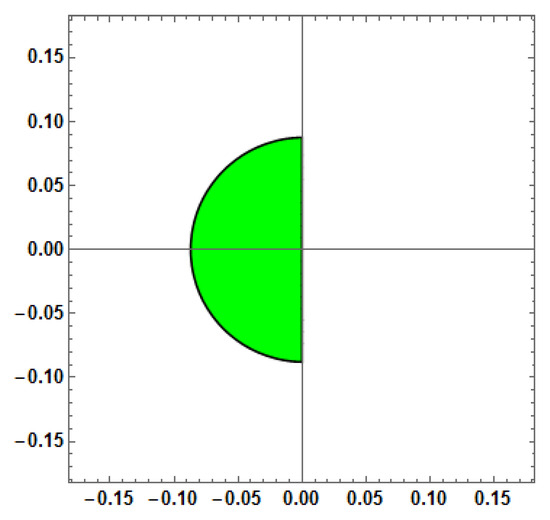
Figure 1. Stability region for Method-1 (Explicit method).

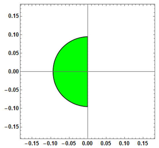
Figure 2. Stability Region for Method-2 (AF = 0) with vs. = h (or w = 1).

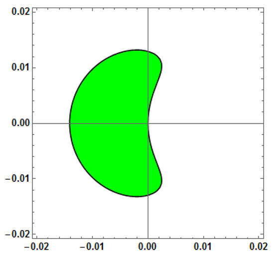
Figure 3. Stability region for Method 2 (AF = 0) with vs. = 1.

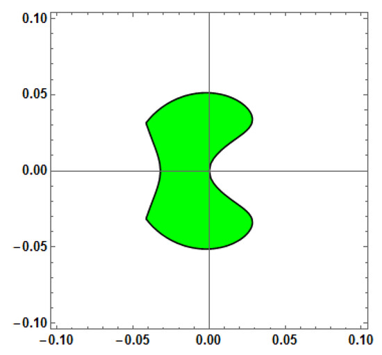
Figure 4. Stability region for Method 2 (AF = 0) with vs. = 100.

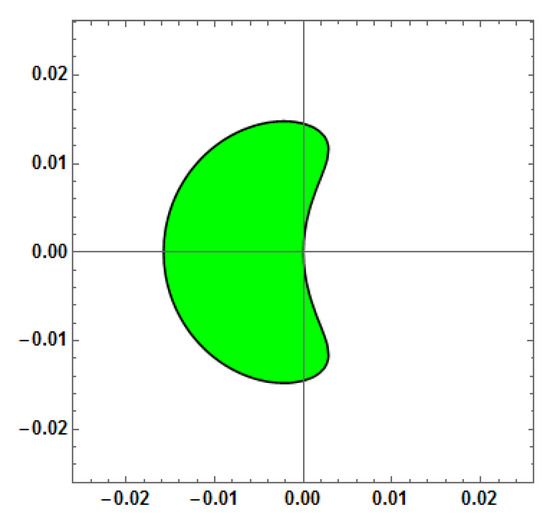
Figure 5. Stability region for Method 2 (AF = 0) with vs. = 1000.

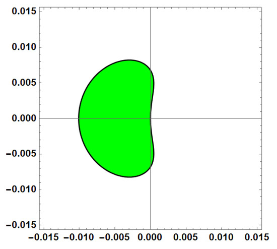
Figure 6. Stability region for Method 3 (AF = 0, PE = 0) with vs. = 1.

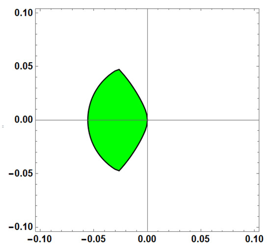
Figure 7. Stability region for Method 3 (AF = 0, PE = 0) with vs. = 100.

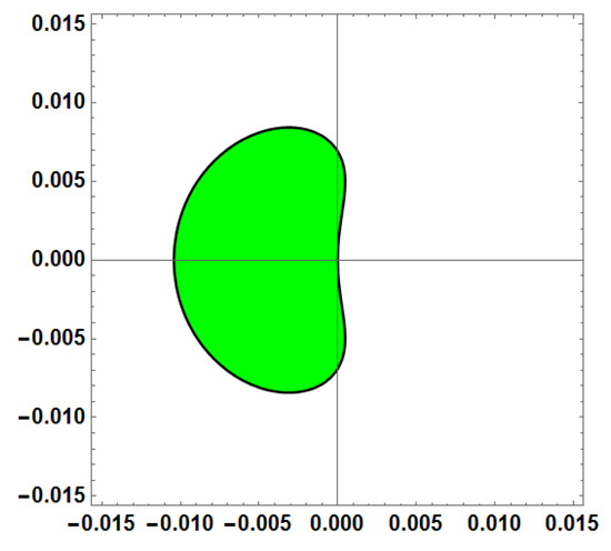
Figure 8. Stability region for Method 3 (AF = 0, PE = 0) with vs. = 1000.

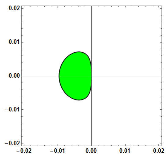
Figure 9. Stability region for Method 4 (AF = 0, PE = 0, D[PE] = 0) with vs. = 1.

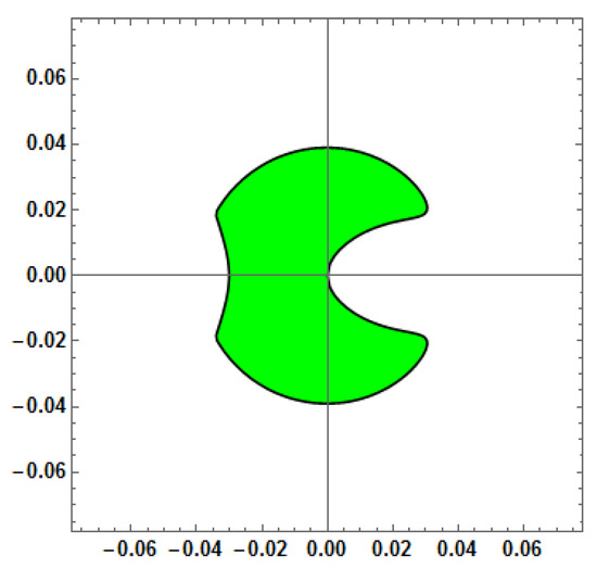
Figure 10. Stability region for Method 4 (AF = 0, PE = 0, D[PE] = 0) with vs. = 100.

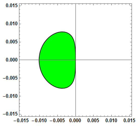
Figure 11. Stability region for Method 4 (AF = 0, PE = 0, D[PE] = 0) with vs. = 1000.

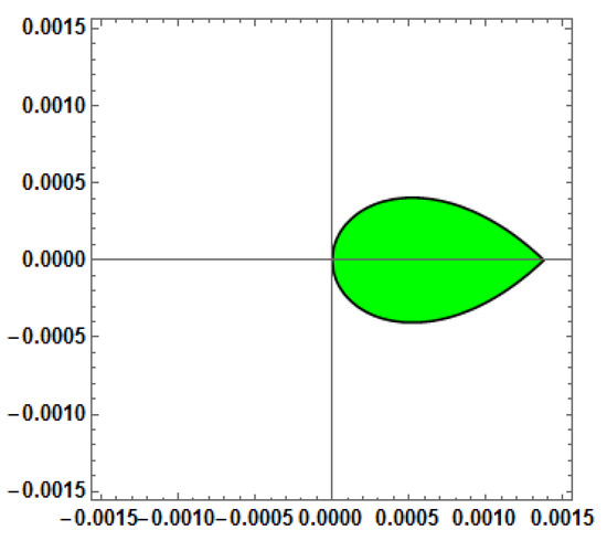
Figure 12. Stability region for Method 5 (AF = 0, PE = 0, D[AF] = 0) with vs. = 1.

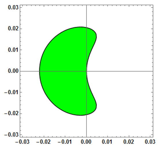
Figure 13. Stability region for Method 5 (AF = 0, PE = 0, D[AF]=0) with vs. = 100.

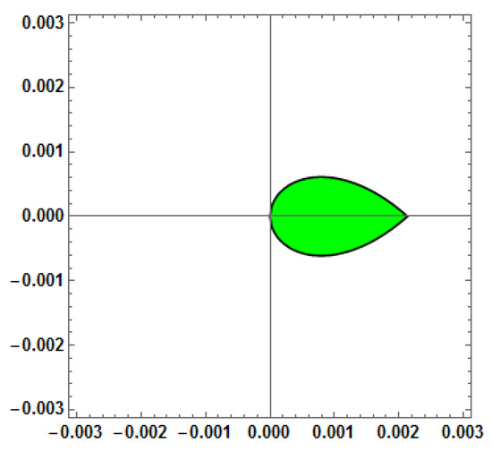
Figure 14. Stability region for Method 5 (AF = 0, PE = 0, D[AF] = 0) with vs. = 1000.

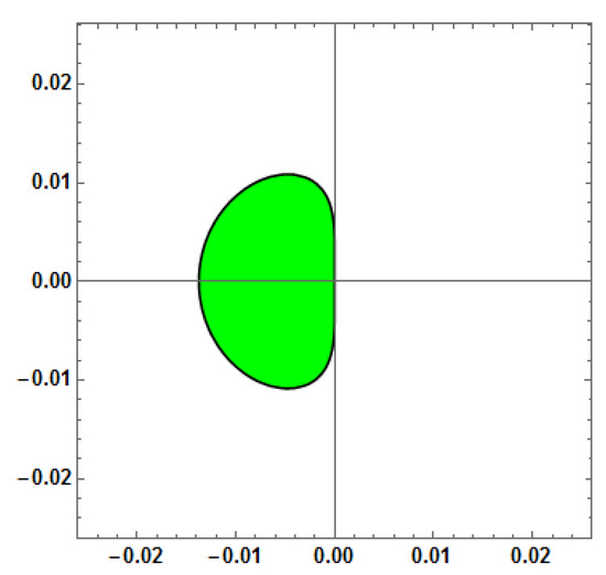
Figure 15. Stability region for Method 6 (AF = 0, PE = 0, D[PE] = 0, D[AF] = 0) with vs. = 1.

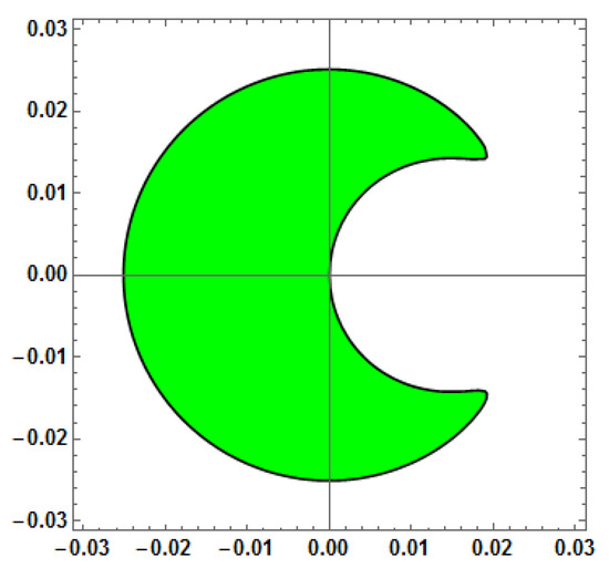
Figure 16. Stability region for Method 6 (AF = 0, PE = 0, D[PE] = 0, D[AF] = 0) with vs. = 100.

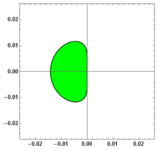
Figure 17. Stability region for Method 6 (AF = 0, PE = 0, D[PE] = 0, D[AF] = 0) with vs. = 1000.

4. Numerical Results

In this section, we solve seven ODE problems with oscillatory solutions and one PDE problem, the Telegraph equation. The error is evaluated using the following formula:

$$\mathrm{Errham}=-{\displaystyle \frac{ln\left(\right|y\left(x_i\right)-y_i\left|\right)}{ln\left(10\right)}}.$$

The ODEs are solved using MATHEMATICA, while the PDE is solved using MATLAB R2017a. For comparison, we have considered three ODE solvers from the Runge–Kutta family [26,27]: the fifth-order Cash–Karp method (RKCash), the fifth-order Fehlberg method (RKFehl), and the fourth-order classical Runge–Kutta method (RK4). To ensure a fair and consistent comparison, all methods-including the developed ones and the benchmark solvers-were implemented in the same software environment, MATHEMATICA (Version number: 11.0.1.0). A uniform step size approach was used across all methods to allow direct and consistent evaluation of error norms and computational performance.

To compute the initial four steps for each problem, Matlab in-built function ode45 is used. The flowchart for the implementation of the derived method is given in Figure 18.

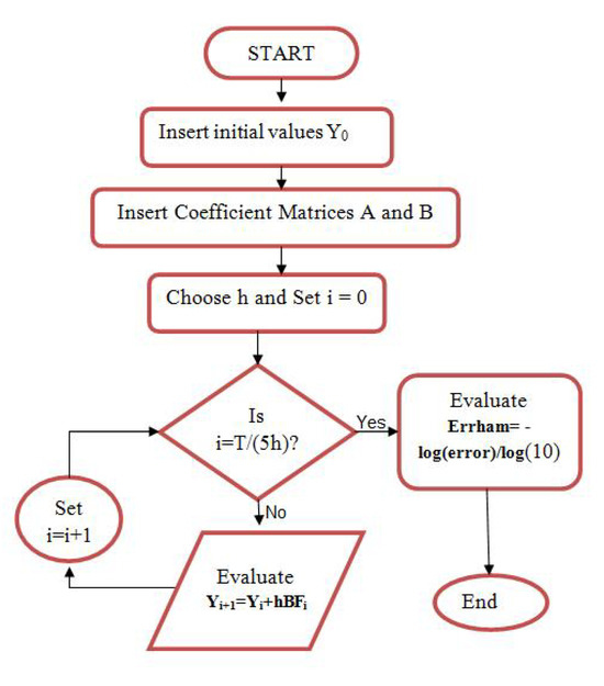
Figure 18. Flowchart for the implementation of block methods.

Example 1.

Stiefel and Bettis [28] studied the almost periodic orbit problem, and it is as follows:

$$\begin{array}{cc}\hfill y_1^{\prime \prime }\left(x\right)& =-y_1\left(x\right)+0.001cos\left(x\right),y_1\left(0\right)=1,y_1^{\prime }\left(0\right)=0,\hfill \\ \hfill y_2^{\prime \prime }\left(x\right)& =-y_2\left(x\right)+0.001sin\left(x\right),y_2\left(0\right)=0,y_2^{\prime }\left(0\right)=0.9995.\hfill \end{array}$$

(31)

The exact solution is

$$\begin{array}{cc}\hfill y_1\left(x\right)& =cos\left(x\right)+0.0005xsin\left(x\right),\hfill \\ \hfill y_2\left(x\right)& =sin\left(x\right)-0.0005xcos\left(x\right).\hfill \end{array}$$

(32)

Using the derived methods $M1-M6$ with $\omega =1$, numerical results have been computed and visualized through Figure 19. The key observations regarding their respective behaviors are outlined below:

• Block methods ($M1,M2,M3,M4,M5,M6$) provide more accurate results compared to the traditional Runge–Kutta methods: Runge–Kutta Fehlberg fifth-order method (RKFehl), Runge–Kutta Cash and Karp fifth-order method (RKCash), and classical fourth-order Runge–Kutta method (RK4).
• Methods $M2$ and $M4$ exhibit the same accuracy, both of which outperform $M1$.
• The results of $M6$ are superior to those of $M2$ and $M4$.
• $M6$ delivers the highest accuracy with a larger step size, achieving this in less CPU time, but it falls behind $M5$ and $M3$ when smaller step sizes are considered.
• $M3$ demonstrates better performance than $M5$.
• Overall, $M3$ achieves the highest accuracy among all the methods.

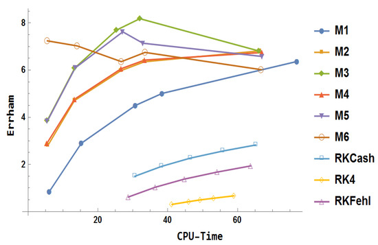
Figure 19. Numerical results for example 1.

Example 2.

The following inhomogeneous linear problem, analyzed by Franco et al. [29], is considered:

$$\begin{array}{cc}\hfill y_1^{\prime \prime }\left(x\right)& =-{\displaystyle \frac{1}{2}}\left({\mu }^2+1\right)y_1\left(x\right)-{\displaystyle \frac{1}{2}}\left({\mu }^2-1\right)y_2\left(x\right),y_1\left(0\right)=1,y_1^{\prime }\left(0\right)=1,\hfill \\ \hfill y_2^{\prime \prime }\left(x\right)& =-{\displaystyle \frac{1}{2}}\left({\mu }^2-1\right)y_1\left(x\right)-{\displaystyle \frac{1}{2}}\left({\mu }^2+1\right)y_2\left(x\right),y_2\left(0\right)=-1,y_2^{\prime }\left(0\right)=-1,\hfill \end{array}$$

(33)

for which the exact solution is given as follows:

$$\begin{array}{cc}\hfill y_1\left(x\right)& =cos\left(x\right)+sin\left(x\right),\hfill \\ \hfill y_2\left(x\right)& =-cos\left(x\right)-sin\left(x\right).\hfill \end{array}$$

(34)

In this case, $\mu ={10}^4$, the investigation interval is $[0,10,000]$, and the numerical solution is computed with $\omega =1$.

The observations on computational outcomes plotted in Figure 20 are as follows:

• Among the Runge–Kutta methods considered, RK4 is the least accurate, while the explicit block method $M1$ provides more accurate results.
• RKCash outperforms RKFehl, but M1 surpasses both methods by a significant margin.
• M2 shows higher accuracy than M1.
• Methods M5 and M4 initially exhibit the same accuracy, but M4 slightly outperforms M5 when the step size is reduced.
• M3 performs better than both M5 and M1.
• The results of M6 are marginally better than those of M5.
• On average, M3 achieves the highest accuracy among all the methods.

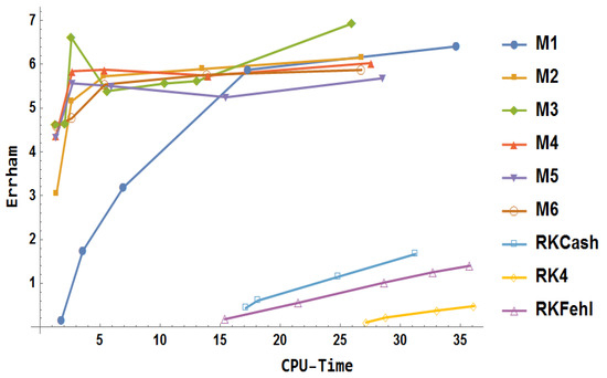
Figure 20. Numerical results for example 2.

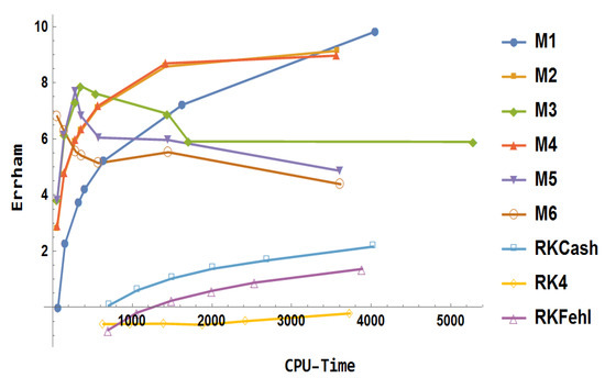
Example 3.

Considering the Franco and Palacios problem [30]:

$$\begin{array}{cc}\hfill y_1^{\prime \prime }\left(x\right)& =-y_1\left(x\right)+ϵcos\left(\vartheta x\right),y_1\left(0\right)=1,y_1^{\prime }\left(0\right)=0,\hfill \\ \hfill y_2^{\prime \prime }\left(x\right)& =-y_2\left(x\right)+ϵsin\left(\vartheta x\right),y_2\left(0\right)=0,y_2^{\prime }\left(0\right)=1.\hfill \end{array}$$

(35)

The exact solution is

$$\begin{array}{cc}\hfill y_1\left(x\right)& ={\displaystyle \frac{1-ϵ-{\vartheta }^2}{1-{\vartheta }^2}}cos\left(x\right)+{\displaystyle \frac{ϵ}{1-{\vartheta }^2}}cos\left(\vartheta x\right),\hfill \\ \hfill y_2\left(x\right)& ={\displaystyle \frac{1-ϵ\vartheta -{\vartheta }^2}{1-{\vartheta }^2}}sin\left(x\right)+{\displaystyle \frac{ϵ}{1-{\vartheta }^2}}sin\left(\vartheta x\right),\hfill \end{array}$$

(36)

where $ϵ=0.001$ and $\vartheta =0.01$. This problem is solved numerically using $\omega =max(1,|\vartheta \left|\right)$ for $0\le x\le 10,000$.

The key observations from Figure 21 are outlined below:

• RKCash yields better performance than both RKFehl and RK4.
• The block method $M1$ produces more precise results than the traditional Runge–Kutta methods.
• Method $M6$ surpasses $M1$ in terms of performance.
• $M5$ provides greater accuracy compared to both $M1$ and $M6$.
• $M3$ achieves the highest accuracy when a large step-size is used, but its accuracy remains unchanged regardless of the step-size.
• $M2$ demonstrates a steady improvement in accuracy as the step-size decreases.
• Among all methods, $M4$ is the most accurate.

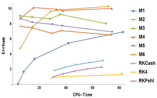
Figure 21. Numerical results for example 3.

Example 4.

The nonlinear orbital problem studied by Simos in [31] is as follows:

$$\begin{array}{cc}\hfill y_1^{\prime \prime }\left(x\right)& =-{\phi }^2{y}_1\left(x\right)+{\displaystyle \frac{2y_1\left(x\right)y_2\left(x\right)-sin\left(2\phi x\right)}{{\left(y_1{\left(x\right)}^2+y_2{\left(x\right)}^2\right)}^{\frac{3}{2}}}},y_1\left(0\right)=1,y_1^{\prime }\left(0\right)=0,\hfill \\ \hfill y_2^{\prime \prime }\left(x\right)& =-{\phi }^2{y}_2\left(x\right)+{\displaystyle \frac{\left(y_1{\left(x\right)}^2-y_2{\left(x\right)}^2\right)-cos\left(2\phi x\right)}{{\left(y_1{\left(x\right)}^2+y_2{\left(x\right)}^2\right)}^{\frac{3}{2}}}},y_2\left(0\right)=0,y_2^{\prime }\left(0\right)=\phi ,\hfill \end{array}$$

(37)

where $\phi =10$. The exact solution is

$$\begin{array}{cc}\hfill y_1\left(x\right)& =cos\left(\phi x\right),\hfill \\ \hfill y_2\left(x\right)& =sin\left(\phi x\right).\hfill \end{array}$$

(38)

The numerical findings for $0\le x\le 10,000$ obtained using $\omega =10$ are shown in Figure 22 and following points summarize the observations:

• RK4 demonstrated no significant improvement despite an increase in CPU time.
• RKCash outperforms both RKFehl and RK4 in terms of overall performance.
• The block method $M1$ delivers more accurate results than the conventional Runge–Kutta methods.
• Method $M2$ exceeds the performance of $M1$ in terms of computational efficiency and accuracy.
• Methods $M3$, $M4$, $M5$, and $M6$ exhibit identical levels of accuracy.
• Methods $M3$, $M4$, $M5$, and $M6$ provide superior accuracy compared to both $M1$ and $M2$.

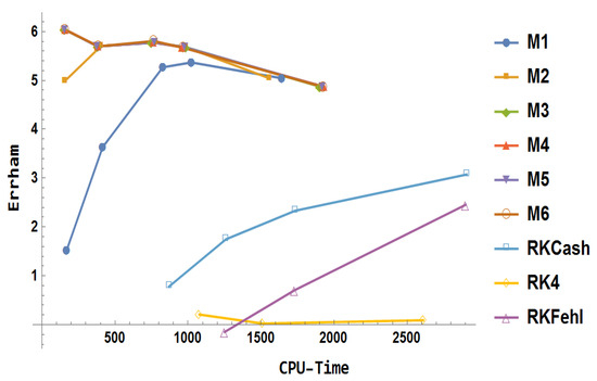
Figure 22. Numerical results for example 4.

Example 5.

Addressing the nonlinear first-order differential problem studied by Petzold [32] as follows:

$$\begin{array}{cc}\hfill y_1^{\prime }\left(x\right)& =\lambda y_2\left(x\right),y_1\left(0\right)=1,\hfill \\ \hfill y_2^{\prime }\left(x\right)& =-\lambda y_1\left(x\right)+{\displaystyle \frac{\alpha }{\lambda }}sin\left(\lambda x\right),y_2\left(0\right)=-{\displaystyle \frac{\alpha }{2{\lambda }^2}},\hfill \end{array}$$

(39)

with the analytical solution

$$\begin{array}{cc}\hfill y_1\left(x\right)& =\left(1-{\displaystyle \frac{\alpha }{2\lambda }}x\right)cos\left(\lambda x\right),\hfill \\ \hfill y_2\left(x\right)& =-\left(1-{\displaystyle \frac{\alpha }{2\lambda }}x\right)sin\left(\lambda x\right)-{\displaystyle \frac{\alpha }{2{\lambda }^2}}cos\left(\lambda x\right),\hfill \end{array}$$

(40)

where $\alpha =100,\lambda =1000$, and the domain of the problem is [0,100]. For this problem, using $\omega =1000$ and plotting results in Figure 23, the following observations are outlined.

Figure 23. Numerical results for example 5.

• RK4 was unable to achieve an acceptable level of accuracy within the given CPU time range.
• RKCash outperforms RKFehl in terms of overall performance.
• The block method $M1$ provides more accurate results than RKCash, with accuracy gradually improving as CPU time increases.
• For very large step-sizes, among the block methods, $M1$ is the least accurate, while $M6$ provides the highest accuracy.
• Methods $M2$ and $M4$ surpass $M1$ in both computational efficiency and accuracy.
• Methods $M2$ and $M4$ demonstrate equivalent performance in terms of accuracy and efficiency.
• Methods $M3$ and $M5$ show similar accuracy initially, but $M3$ exhibits a slight improvement over time.
• Method $M6$ performs better than the others at the beginning but loses its advantage as the process progresses.

Example 6.

Considering the two-body gravitational problem:

$$\begin{array}{cc}\hfill y_1^{\prime \prime }\left(x\right)& =-{\displaystyle \frac{y_1\left(x\right)}{{\left(y_1{\left(x\right)}^2+y_2{\left(x\right)}^2\right)}^{\frac{3}{2}}}},y_1\left(0\right)=1,y_1^{\prime }\left(0\right)=0,\hfill \\ \hfill y_2^{\prime \prime }\left(x\right)& =-{\displaystyle \frac{y_2\left(x\right)}{{\left(y_1{\left(x\right)}^2+y_2{\left(x\right)}^2\right)}^{\frac{3}{2}}}},y_2\left(0\right)=0,y_2^{\prime }\left(0\right)=1.\hfill \end{array}$$

(41)

The true solution is

$$\begin{array}{cc}\hfill y_1\left(x\right)& =cos\left(x\right),\hfill \\ \hfill y_2\left(x\right)& =sin\left(x\right).\hfill \end{array}$$

(42)

Using $\omega =1$, Figure 24 shows numerical results for $0\le x\le 10,000$. The comparison is summarized in the following points.

• The Runge–Kutta methods (RK4, RKCash, and RKFehl) exhibit minimal improvement, maintaining a constant level of performance without significant advancement.
• The block method $M1$ demonstrates superior accuracy when compared to the conventional Runge–Kutta methods.
• Initially, $M6$ outperforms $M1$, but as the step-size is reduced, $M6$ reaches a saturation point, while $M1$ continues to show improvement with smaller step-sizes.
• The block method $M5$ delivers more precise results than $M6$, showing a clear advantage in accuracy.
• Method $M3$ surpasses $M5$ in terms of both accuracy and computational efficiency.
• Method $M2$ outperforms $M3$ in terms of overall accuracy and efficiency.
• In comparison to other methods, $M4$ provides the highest accuracy when a very large step size is employed.

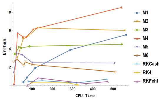
Figure 24. Numerical results for example 6.

Example 7.

We consider the perturbed two-body Kepler’s problem:

$$y_1^{\prime \prime }\left(x\right)=-{\displaystyle \frac{y_1\left(x\right)}{{\left(y_1{\left(x\right)}^2+y_2{\left(x\right)}^2\right)}^{3/2}}}-\mu \left(\mu +2\right){\displaystyle \frac{y_1\left(x\right)}{{\left(y_1{\left(x\right)}^2+y_2{\left(x\right)}^2\right)}^{5/2}}},$$

$$y_1\left(0\right)=1,y_1^{\prime }\left(0\right)=0,$$

$$y_2^{\prime \prime }\left(x\right)=-{\displaystyle \frac{y_2\left(x\right)}{{\left(y_1{\left(x\right)}^2+y_2{\left(x\right)}^2\right)}^{3/2}}}-\mu \left(\mu +2\right){\displaystyle \frac{y_2\left(x\right)}{{\left(y_1{\left(x\right)}^2+y_2{\left(x\right)}^2\right)}^{5/2}}},$$

$$y_2\left(0\right)=0,y_2^{\prime }\left(0\right)=1+\mu$$

The exact solution is:

$$y_1\left(x\right)=cos(x+\mu x),y_2\left(x\right)=sin(x+\mu x).$$

For this problem, we use:

$$\omega =\sqrt{1+\mu \left(\mu +2\right)}.$$

The domain of the system of differential equation is $0\le x\le 10,000$ with $\mu =0.1$.

From Figure 25, it is observed that:

• The Runge–Kutta methods (RK4, RKFehl, and RKCash) show limited improvement in both accuracy and efficiency, with RK4 performing the worst.
• The block method $M1$ outperforms all Runge–Kutta methods in terms of accuracy.
• $M6$ delivers superior performance compared to $M1$, especially with larger step-sizes, achieving higher accuracy initially, but its advantage diminishes as the process progresses.
• $M5$ achieves more accurate results than $M6$ and maintains superior performance in terms of both precision and computational efficiency.
• $M3$ surpasses $M5$ with improved results, especially leveling up the accuracy.
• $M2$ outperforms $M3$ in both accuracy and efficiency, providing the best overall performance across different step sizes.
• $M2$ and $M4$ deliver equivalent performance, both excelling in accuracy and efficiency, making either method an optimal choice for high-precision applications.

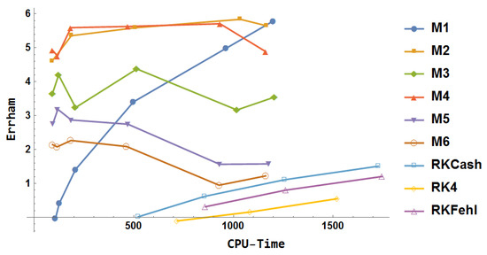
Figure 25. Numerical results for example 7.

Example 8.

Consider the hyperbolic telegraph equation

$$u_{tt}(z,t)+2a{u}_t(z,t)+b^{2}u(z,t)=u_{zz}(z,t)+f(z,t),0\le z\le 1,t\ge 0.$$

The initial and boundary conditions are given by:

$$u(z,0)=sin\left(z\right),u_t(z,0)=0,0\le z\le 1;$$

$$u(0,t)=0,u(1,t)=cos\left(t\right)sin\left(1\right),t\ge 0.$$

The parameters are chosen as $a=6$, $b=2$, and

$$f(z,t)=-2asin\left(t\right)sin\left(z\right)+b^{2}cos\left(t\right)sin\left(z\right).$$

The analytic solution is

$$u(z,t)=cos\left(t\right)sin\left(z\right).$$

For block methods, the parameter $w=1$ is chosen. The following observations can be made:

• The results in Table 1 demonstrate that the block method, implemented using the algorithm presented in [33], significantly outperforms the results reported in [34], which considered SSP-RK54.
  Table 1. Comparison of $L_{\infty }$ error.

  t	[34]	M1	M2	M3	M4	M5	M6
  0.2	$5.2412\times {10}^{-6}$	$1.0977\times {10}^{-9}$	$9.7877\times {10}^{-13}$	$1.1102\times {10}^{-16}$	$1.1102\times {10}^{-16}$	$1.1102\times {10}^{-15}$	$1.1102\times {10}^{-15}$
  0.4	$8.6095\times {10}^{-6}$	$6.9168\times {10}^{-8}$	$2.6006\times {10}^{-10}$	$1.1102\times {10}^{-16}$	$2.2204\times {10}^{-16}$	$8.8818\times {10}^{-16}$	$8.8818\times {10}^{-16}$
  0.6	$1.2529\times {10}^{-5}$	$7.6740\times {10}^{-7}$	$7.1087\times {10}^{-9}$	$1.1102\times {10}^{-16}$	$2.2204\times {10}^{-16}$	$2.4425\times {10}^{-15}$	$2.4425\times {10}^{-15}$
  0.8	$2.0274\times {10}^{-5}$	$4.1529\times {10}^{-6}$	$7.8154\times {10}^{-8}$	$1.1102\times {10}^{-16}$	$1.1102\times {10}^{-16}$	$1.1102\times {10}^{-15}$	$1.1102\times {10}^{-15}$
  1.0	$2.7555\times {10}^{-5}$	$1.5076\times {10}^{-5}$	$5.3307\times {10}^{-7}$	$1.6653\times {10}^{-16}$	$2.2204\times {10}^{-16}$	$1.3878\times {10}^{-15}$	$1.3878\times {10}^{-15}$

• The error analysis Figure 26 for $t=1$ indicates that $M2$ achieves better accuracy compared to $M1$.
  

  Figure 26. Numerical results for example 8.
• Method $M5$ exhibits a significantly higher accuracy than $M2$, with a considerable margin of improvement.
• Methods $M5$ and $M6$ display equivalent accuracy over the spatial grid.
• Method $M4$ surpasses $M5$ in performance across all considered time values.
• Methods $M3$ and $M4$ demonstrate almost comparable accuracy, with a slight advantage observed for $M3$.
• The CPU time required for $t=1$ varies among the methods: $M1$ completes in 0.003172 s, $M2$ in 0.010569 s, $M3$ in 0.010235 s, $M4$ in 0.011391 s, $M5$ in 0.015868 s, and $M6$ in 0.013777 s.
• Overall, $M3$ demonstrated the best performance among the other methods.

Based on the numerical problems considered in the study, the overall performance and interpretation are summarized in the following Table 2.

Table 2. Performance Summary of Numerical Methods.

Method	Order	AF	PhEr	First Order Derivative of AF	First Order Derivative of PhEr	Rank Based (on Performance)
$M1$	5	6	4	×	×	5
$M2$	4	0	6	×	×	2
$M3$	5	0	0	×	×	2
$M4$	4	0	0	×	✓	1
$M5$	5	0	0	✓	×	3
$M6$	5	0	0	✓	✓	4

5. Conclusions

Overall, the block methods significantly outperform traditional Runge–Kutta methods, with $M1$ showing notable improvement over RK4, RKFehl, and RKCash. As we move to more advanced block methods, such as $M2$, $M3$, $M4$, $M5$, and $M6$, there is a consistent increase in both accuracy and computational efficiency. There was a close competition among $M2$, $M3$, and $M4$, while $M5$ and $M6$ performed better than $M1$ but fell short compared to the other methods. No single method emerged as the definitive winner, as the performance of numerical methods depends heavily on the type of problem being addressed. For partial differential equations (PDEs), $M3$ and $M4$ delivered the best results. Among these, $M4$ consistently demonstrated its effectiveness and superiority in most cases. This study not only evaluates the performance of the methods but also broadens the scope of applications for modified explicit block methods.

Appendix A.1. Amplification-Fitted and Phase Fitted Block Method: Method 3

For Method $M3$, the elimination of $AF$ will lead to (22) and equating $PhEr$ to zero results in following equations:

$$\begin{array}{cc}\hfill b_4& =-{\displaystyle \frac{b_{1}tan\left(4v\right)}{cos\left(3v\right)tan\left(4v\right)-sin\left(3v\right)}}\hfill \\ \hfill & -{\displaystyle \frac{b_2(cos\left(v\right)tan\left(4v\right)-sin\left(v\right))}{cos\left(3v\right)tan\left(4v\right)-sin\left(3v\right)}}-{\displaystyle \frac{b_3(cos\left(2v\right)tan\left(4v\right)-sin\left(2v\right))}{cos\left(3v\right)tan\left(4v\right)-sin\left(3v\right)}}\hfill \\ \hfill & -{\displaystyle \frac{-2cos\left(v\right)-3cos\left(2v\right)-4cos\left(3v\right)-5cos\left(4v\right)+15cos\left(5v\right)}{15vs.(sin(3v)-cos(3v)tan(4v\left)\right)}}\hfill \\ \hfill & -{\displaystyle \frac{-2sin\left(v\right)tan\left(4v\right)-3sin\left(2v\right)tan\left(4v\right)}{15vs.(sin(3v)-cos(3v)tan(4v\left)\right)}}\hfill \\ \hfill & +{\displaystyle \frac{-4sin\left(3v\right)tan\left(4v\right)-5sin\left(4v\right)tan\left(4v\right)+15sin\left(5v\right)tan\left(4v\right)-1}{15vs.(sin(3v)-cos(3v)tan(4v\left)\right)}},\hfill \\ \hfill \\ \hfill b_6& =-b_{7}cot\left(4v\right)(cos\left(v\right)tan\left(4v\right)-sin\left(v\right))-b_{8}cot\left(4v\right)(cos\left(2v\right)tan\left(4v\right)-sin\left(2v\right))\hfill \\ \hfill & -b_{9}cot\left(4v\right)(cos\left(3v\right)tan\left(4v\right)-sin\left(3v\right))\hfill \\ \hfill & -{\displaystyle \frac{1}{15v}}(cot\left(4v\right)(2cos\left(v\right)+3cos\left(2v\right)+4cos\left(3v\right)+5cos\left(4v\right)-15cos\left(6v\right)+2sin\left(v\right)tan\left(4v\right)\hfill \\ \hfill & +3sin\left(2v\right)tan\left(4v\right)+4sin\left(3v\right)tan\left(4v\right)+5sin\left(4v\right)tan\left(4v\right)-15sin\left(6v\right)tan\left(4v\right)+1\left)\right),\hfill \\ \hfill \\ \hfill b_{11}& =-b_{12}cot\left(4v\right)(cos\left(v\right)tan\left(4v\right)-sin\left(v\right))-b_{13}cot\left(4v\right)(cos\left(2v\right)tan\left(4v\right)-sin\left(2v\right))\hfill \\ \hfill & -b_{14}cot\left(4v\right)(cos\left(3v\right)tan\left(4v\right)-sin\left(3v\right))\hfill \\ \hfill & -{\displaystyle \frac{1}{15v}}(cot\left(4v\right)(2cos\left(v\right)+3cos\left(2v\right)+4cos\left(3v\right)+5cos\left(4v\right)-15cos\left(7v\right)+2sin\left(v\right)tan\left(4v\right)\hfill \\ \hfill & +3sin\left(2v\right)tan\left(4v\right)+4sin\left(3v\right)tan\left(4v\right)+5sin\left(4v\right)tan\left(4v\right)-15sin\left(7v\right)tan\left(4v\right)+1\left)\right),\hfill \\ \hfill b_{16}& =-b_{17}cot\left(4v\right)(cos\left(v\right)tan\left(4v\right)-sin\left(v\right))-b_{18}cot\left(4v\right)(cos\left(2v\right)tan\left(4v\right)-sin\left(2v\right))\hfill \\ \hfill & -b_{19}cot\left(4v\right)(cos\left(3v\right)tan\left(4v\right)-sin\left(3v\right))\hfill \\ \hfill & -{\displaystyle \frac{1}{15v}}(cot\left(4v\right)(2cos\left(v\right)+3cos\left(2v\right)+4cos\left(3v\right)+5cos\left(4v\right)-15cos\left(8v\right)+2sin\left(v\right)tan\left(4v\right)\hfill \\ \hfill & +3sin\left(2v\right)tan\left(4v\right)+4sin\left(3v\right)tan\left(4v\right)+5sin\left(4v\right)tan\left(4v\right)-15sin\left(8v\right)tan\left(4v\right)+1\left)\right),\hfill \\ \hfill \\ \hfill b_{21}& =-b_{22}cot\left(4v\right)(cos\left(v\right)tan\left(4v\right)-sin\left(v\right))-b_{23}cot\left(4v\right)(cos\left(2v\right)tan\left(4v\right)-sin\left(2v\right))\hfill \\ \hfill & -b_{24}cot\left(4v\right)(cos\left(3v\right)tan\left(4v\right)-sin\left(3v\right))\hfill \\ \hfill & -{\displaystyle \frac{1}{15v}}(cot\left(4v\right)(2cos\left(v\right)+3cos\left(2v\right)+4cos\left(3v\right)+5cos\left(4v\right)-15cos\left(9v\right)+2sin\left(v\right)tan\left(4v\right)\hfill \\ \hfill & +3sin\left(2v\right)tan\left(4v\right)+4sin\left(3v\right)tan\left(4v\right)+5sin\left(4v\right)tan\left(4v\right)-15sin\left(9v\right)tan\left(4v\right)+1\left)\right).\hfill \end{array}$$

(A1)

To continue the evaluation of the remaining unknown components of the matrix, the local truncation error is minimized by setting the first three leading coefficients in the series expansion equal to zero.

$$b_2=-{\displaystyle \frac{1681}{1080}},b_3={\displaystyle \frac{337}{90}},b_8={\displaystyle \frac{1277}{45}},$$

$$b_9=-{\displaystyle \frac{2791}{108}},b_{13}={\displaystyle \frac{9811}{90}},b_{18}={\displaystyle \frac{13709}{45}},$$

$$b_{23}={\displaystyle \frac{12677}{18}},b_{14}=-{\displaystyle \frac{102271}{1080}},b_{19}=-{\displaystyle \frac{137051}{540}},$$

$$b_{24}=-{\displaystyle \frac{613783}{1080}},b_1={\displaystyle \frac{767}{2160}},b_7=-{\displaystyle \frac{7781}{540}},$$

$$b_{12}=-{\displaystyle \frac{63193}{1080}},b_{17}=-{\displaystyle \frac{91277}{540}},b_{22}=-{\displaystyle \frac{86429}{216}}.$$

By using these values, the coefficient matrix obtained after calculation is $B_3$.

$$\begin{array}{cc}\hfill B_3\left[14\right]=& -{\displaystyle \frac{sec\left(\frac{v}{2}\right)}{2160v}}(5493vs.cos\left({\displaystyle \frac{v}{2}}\right)\hfill \\ \hfill & +5493vs.cos\left({\displaystyle \frac{3v}{2}}\right)-2595vs.cos\left({\displaystyle \frac{5v}{2}}\right)\hfill \\ \hfill & +767vs.cos\left({\displaystyle \frac{7v}{2}}\right)+720sin\left({\displaystyle \frac{v}{2}}\right)\hfill \\ \hfill & -864sin\left({\displaystyle \frac{3v}{2}}\right)-432sin\left({\displaystyle \frac{5v}{2}}\right)\hfill \\ \hfill & -144sin\left({\displaystyle \frac{7v}{2}}\right)),\hfill \end{array}$$

$$\begin{array}{cc}\hfill B_3\left[15\right]=& {\displaystyle \frac{sec\left(\frac{v}{2}\right)}{2160v}}(576sin\left({\displaystyle \frac{v}{2}}\right)\hfill \\ \hfill & +1728sin\left({\displaystyle \frac{3v}{2}}\right)-144sin\left({\displaystyle \frac{5v}{2}}\right)\hfill \\ \hfill & +5493vs.cos\left({\displaystyle \frac{v}{2}}\right)-2595vs.cos\left({\displaystyle \frac{3v}{2}}\right)\hfill \\ \hfill & +767vs.cos\left({\displaystyle \frac{5v}{2}}\right)),\hfill \end{array}$$

$$\begin{array}{cc}\hfill B_3\left[21\right]=& {\displaystyle \frac{1}{540vs.\left(cos\left(\frac{v}{2}\right)+cos\left(\frac{3v}{2}\right)+cos\left(\frac{5v}{2}\right)+cos\left(\frac{7v}{2}\right)\right)}}(\hfill \\ \hfill & 6412vs.cos\left({\displaystyle \frac{v}{2}}\right)-7543vs.cos\left({\displaystyle \frac{3v}{2}}\right)\hfill \\ \hfill & +7781vs.cos\left({\displaystyle \frac{5v}{2}}\right)-180sin\left({\displaystyle \frac{v}{2}}\right)\hfill \\ \hfill & -324sin\left({\displaystyle \frac{3v}{2}}\right)+108sin\left({\displaystyle \frac{5v}{2}}\right)\hfill \\ \hfill & +36sin\left({\displaystyle \frac{7v}{2}}\right)),\hfill \end{array}$$

$$\begin{array}{cc}\hfill B_3\left[25\right]=& {\displaystyle \frac{180cot\left(4v\right)}{540v}}-{\displaystyle \frac{\frac{1}{4}csc\left(v\right)sec\left(v\right)sec\left(2v\right)}{540v}}(-7781vs.sin\left(v\right)\hfill \\ \hfill & +15324vs.sin\left(2v\right)-13955vs.sin\left(3v\right)-72cos\left(v\right)\hfill \\ \hfill & -108cos\left(2v\right)-144cos\left(3v\right)+540cos\left(6v\right)-36),\hfill \end{array}$$

$$\begin{array}{cc}\hfill B_3\left[31\right]=& {\displaystyle \frac{1}{1080vs.\left(cos\left(\frac{v}{2}\right)+cos\left(\frac{3v}{2}\right)+cos\left(\frac{5v}{2}\right)+cos\left(\frac{7v}{2}\right)\right)}}(47732vs.cos\left({\displaystyle \frac{v}{2}}\right)\hfill \\ \hfill & -54539vs.cos\left({\displaystyle \frac{3v}{2}}\right)+63193vs.cos\left({\displaystyle \frac{5v}{2}}\right)\hfill \\ \hfill & -360sin\left({\displaystyle \frac{v}{2}}\right)-648sin\left({\displaystyle \frac{3v}{2}}\right)\hfill \\ \hfill & -864sin\left({\displaystyle \frac{5v}{2}}\right)+72sin\left({\displaystyle \frac{7v}{2}}\right)),\hfill \end{array}$$

$$\begin{array}{cc}\hfill B_3\left[35\right]=& {\displaystyle \frac{1440cot\left(4v\right)}{4320v}}-{\displaystyle \frac{csc\left(v\right)sec\left(v\right)sec\left(2v\right)}{4320v}}(-63193vs.sin\left(v\right)\hfill \\ \hfill & +117732vs.sin\left(2v\right)-102271vs.sin\left(3v\right)-144cos\left(v\right)-216cos\left(2v\right)\hfill \\ \hfill & -288cos\left(3v\right)+1080cos\left(7v\right)-72),\hfill \end{array}$$

$$\begin{array}{cc}\hfill B_3\left[41\right]=& -{\displaystyle \frac{1}{540vs.\left(cos\left(\frac{v}{2}\right)+cos\left(\frac{3v}{2}\right)+cos\left(\frac{5v}{2}\right)+cos\left(\frac{7v}{2}\right)\right)}}(-63820vs.cos\left({\displaystyle \frac{v}{2}}\right)\hfill \\ \hfill & +73231vs.cos\left({\displaystyle \frac{3v}{2}}\right)-91277vs.cos\left({\displaystyle \frac{5v}{2}}\right)\hfill \\ \hfill & +180sin\left({\displaystyle \frac{v}{2}}\right)+324sin\left({\displaystyle \frac{3v}{2}}\right)\hfill \\ \hfill & +432sin\left({\displaystyle \frac{5v}{2}}\right)+504sin\left({\displaystyle \frac{7v}{2}}\right)),\hfill \end{array}$$

$$\begin{array}{cc}\hfill B_3\left[45\right]=& {\displaystyle \frac{720cot\left(4v\right)}{2160v}}{\displaystyle \frac{csc\left(v\right)sec\left(v\right)sec\left(2v\right)}{2160v}}(-91277vs.sin\left(v\right)\hfill \\ \hfill & +164508vs.sin\left(2v\right)-137051vs.sin\left(3v\right)-72cos\left(v\right)-108cos\left(2v\right)\hfill \\ \hfill & -144cos\left(3v\right)+540cos\left(8v\right)-36),\hfill \end{array}$$

$$\begin{array}{cc}\hfill B_3\left[51\right]=& -{\displaystyle \frac{1}{1080vs.\left(cos\left(\frac{v}{2}\right)+cos\left(\frac{3v}{2}\right)+cos\left(\frac{5v}{2}\right)+cos\left(\frac{7v}{2}\right)\right)}}(-285308vs.cos\left({\displaystyle \frac{v}{2}}\right)\hfill \\ \hfill & +328475vs.cos\left({\displaystyle \frac{3v}{2}}\right)-432145vs.cos\left({\displaystyle \frac{5v}{2}}\right)\hfill \\ \hfill & +360sin\left({\displaystyle \frac{v}{2}}\right)+648sin\left({\displaystyle \frac{3v}{2}}\right)\hfill \\ \hfill & +864sin\left({\displaystyle \frac{5v}{2}}\right)+1008sin\left({\displaystyle \frac{7v}{2}}\right)\hfill \\ \hfill & +1080sin\left({\displaystyle \frac{9v}{2}}\right)),\hfill \end{array}$$

$$\begin{array}{cc}\hfill B_3\left[55\right]=& {\displaystyle \frac{1440cot\left(4v\right)}{4320v}}-{\displaystyle \frac{csc\left(v\right)sec\left(v\right)sec\left(2v\right)}{4320v}}(-432145vs.sin\left(v\right)\hfill \\ \hfill & +760620vs.sin\left(2v\right)-613783vs.sin\left(3v\right)-144cos\left(v\right)-216cos\left(2v\right)\hfill \\ \hfill & -288cos\left(3v\right)+1080cos\left(9v\right)-72).\hfill \end{array}$$

The remaining elements of matrix $B_3$ are as follows:

$$\begin{array}{cc}\hfill B_3\left[15\right]=b_5=& {\displaystyle \frac{sec\left(\frac{v}{2}\right)}{2160v}}(576sin\left({\displaystyle \frac{v}{2}}\right)\hfill \\ \hfill & +1728sin\left({\displaystyle \frac{3v}{2}}\right)-144sin\left({\displaystyle \frac{5v}{2}}\right)\hfill \\ \hfill & +5493vs.cos\left({\displaystyle \frac{v}{2}}\right)-2595vs.cos\left({\displaystyle \frac{3v}{2}}\right)\hfill \\ \hfill & +767vs.cos\left({\displaystyle \frac{5v}{2}}\right)),\hfill \end{array}$$

$$\begin{array}{cc}\hfill B_3\left[25\right]=b_{10}=& {\displaystyle \frac{180cot\left(4v\right)}{540v}}-{\displaystyle \frac{\frac{1}{4}csc\left(v\right)sec\left(v\right)sec\left(2v\right)}{540v}}(-7781vs.sin\left(v\right)\hfill \\ \hfill & +15324vs.sin\left(2v\right)-13955vs.sin\left(3v\right)-72cos\left(v\right)\hfill \\ \hfill & -108cos\left(2v\right)-144cos\left(3v\right)+540cos\left(6v\right)-36),\hfill \end{array}$$

$$\begin{array}{cc}\hfill B_3\left[35\right]=b_{15}=& {\displaystyle \frac{1440cot\left(4v\right)}{4320v}}-{\displaystyle \frac{csc\left(v\right)sec\left(v\right)sec\left(2v\right)}{4320v}}(-63193vs.sin\left(v\right)\hfill \\ \hfill & +117732vs.sin\left(2v\right)-102271vs.sin\left(3v\right)-144cos\left(v\right)-216cos\left(2v\right)\hfill \\ \hfill & -288cos\left(3v\right)+1080cos\left(7v\right)-72),\hfill \end{array}$$

$$\begin{array}{cc}\hfill B_3\left[45\right]=b_{20}=& {\displaystyle \frac{720cot\left(4v\right)}{2160v}}{\displaystyle \frac{csc\left(v\right)sec\left(v\right)sec\left(2v\right)}{2160v}}(-91277vs.sin\left(v\right)\hfill \\ \hfill & +164508vs.sin\left(2v\right)-137051vs.sin\left(3v\right)-72cos\left(v\right)-108cos\left(2v\right)\hfill \\ \hfill & -144cos\left(3v\right)+540cos\left(8v\right)-36),\hfill \end{array}$$

$$\begin{array}{cc}\hfill B_3\left[55\right]=b_{25}=& {\displaystyle \frac{1440cot\left(4v\right)}{4320v}}-{\displaystyle \frac{csc\left(v\right)sec\left(v\right)sec\left(2v\right)}{4320v}}(-432145vs.sin\left(v\right)\hfill \\ \hfill & +760620vs.sin\left(2v\right)-613783vs.sin\left(3v\right)-144cos\left(v\right)-216cos\left(2v\right)\hfill \\ \hfill & -288cos\left(3v\right)+1080cos\left(9v\right)-72).\hfill \end{array}$$

Appendix A.2. Amplification-Fitted and Phase Fitted Block Method with Vanished First Derivative of Phase-Error: Method 4

The elements of matrix $B3$ are as follows:

$$\begin{array}{cc}\hfill B_4\left[13\right]=& -{\displaystyle \frac{{sin}^2\left(\frac{v}{2}\right){csc}^3\left(v\right)}{2160v^2(2cos\left(2v\right)+1)}}[-2122v^{2}sin\left(v\right)\hfill \\ \hfill & -9613v^{2}sin\left(2v\right)-7018v^{2}sin\left(3v\right)-4423v^{2}sin\left(4v\right)-1828v^{2}sin\left(5v\right)\hfill \\ \hfill & +767v^{2}sin\left(6v\right)+4608vs.-576sin\left(v\right)-1296sin\left(2v\right)-2304sin\left(3v\right)\hfill \\ \hfill & -3600sin\left(4v\right)-2160sin\left(5v\right)+8640vs.cos\left(v\right)+7776vs.cos\left(2v\right)\hfill \\ \hfill & +5616vs.cos\left(3v\right)+5760vs.cos\left(4v\right)+2736vs.cos\left(5v\right)+144vs.cos\left(6v\right)],\hfill \end{array}$$

$$\begin{array}{cc}\hfill B_4\left[14\right]=& {\displaystyle \frac{{sin}^2\left(\frac{v}{2}\right){csc}^3\left(v\right)}{1080v^2(2cos\left(2v\right)+1)}}[-1828v^{2}sin\left(v\right)\hfill \\ \hfill & -1975v^{2}sin\left(2v\right)-4423v^{2}sin\left(3v\right)-1828v^{2}sin\left(4v\right)\hfill \\ \hfill & +767v^{2}sin\left(5v\right)+4608vs.-648sin\left(v\right)-1440sin\left(2v\right)-2448sin\left(3v\right)\hfill \\ \hfill & -2232sin\left(4v\right)-1800sin\left(5v\right)-1080sin\left(6v\right)+9216vs.cos\left(v\right)+7200vs.cos\left(2v\right)\hfill \\ \hfill & +6768vs.cos\left(3v\right)+4104vs.cos\left(4v\right)+2304vs.cos\left(5v\right)+1080vs.cos\left(6v\right)],\hfill \end{array}$$

$$\begin{array}{cc}\hfill B_4\left[15\right]=& -{\displaystyle \frac{{sin}^2\left(\frac{v}{2}\right){csc}^3\left(v\right)}{2160v^2(2cos\left(2v\right)+1)}}[-294v^{2}sin\left(v\right)\hfill \\ \hfill & -4423v^{2}sin\left(2v\right)-1828v^{2}sin\left(3v\right)+767v^{2}sin\left(4v\right)\hfill \\ \hfill & +4752vs.-576sin\left(v\right)-1296sin\left(2v\right)-2304sin\left(3v\right)-3600sin\left(4v\right)\hfill \\ \hfill & -2160sin\left(5v\right)+7056vs.cos\left(v\right)+5472vs.cos\left(2v\right)+5616vs.cos\left(3v\right)\hfill \\ \hfill & +8064vs.cos\left(4v\right)+4320vs.cos\left(5v\right)],\hfill \end{array}$$

$$\begin{array}{cc}\hfill B_4\left[21\right]=& {\displaystyle \frac{csc\left(\frac{v}{2}\right){sec}^3\left(\frac{v}{2}\right)}{8640v^2(3cos\left(2v\right)+cos\left(4v\right)+3)}}[15562v^{2}sin\left(v\right)\hfill \\ \hfill & +15800v^{2}sin\left(2v\right)-7305v^{2}sin\left(3v\right)+238v^{2}sin\left(4v\right)\hfill \\ \hfill & +7781v^{2}sin\left(5v\right)-1692vs.+144sin\left(v\right)+324sin\left(2v\right)+576sin\left(3v\right)\hfill \\ \hfill & +900sin\left(4v\right)+1080sin\left(5v\right)+540sin\left(6v\right)-3240vs.cos\left(v\right)-2484vs.cos\left(2v\right)\hfill \\ \hfill & -1944vs.cos\left(3v\right)-1980vs.cos\left(4v\right)-2304vs.cos\left(5v\right)-1116vs.cos\left(6v\right)],\hfill \end{array}$$

$$\begin{array}{cc}\hfill B_4\left[24\right]=& {\displaystyle \frac{1}{135v^2(7sin\left(v\right)-sin\left(7v\right))}}[2vs.(v{sin}^3\left(v\right)(-91944cos\left(v\right)\hfill \\ \hfill & +7781(3cos(2v)+2)-30648cos\left(3v\right))-9(14cos\left(v\right)-66cos\left(2v\right)\hfill \\ \hfill & +5cos\left(3v\right)+4cos\left(4v\right)+3cos\left(5v\right)+3cos\left(6v\right)+2cos\left(7v\right)+15cos\left(10v\right)\left)\right)\hfill \\ \hfill & -9(4sin(v)+18sin(2v)+2sin(3v)+2sin(4v)+2sin(5v)+3sin(6v)\hfill \\ \hfill & +4sin\left(7v\right)+5(8v+sin(8v)-3sin(10v\left)\right)\left)\right],\hfill \end{array}$$

$$\begin{array}{cc}\hfill B_4\left[25\right]=& {\displaystyle \frac{1}{4320v^2(3cos\left(2v\right)+cos\left(4v\right)+3)}}[csc\left({\displaystyle \frac{v}{2}}\right){sec}^3\left({\displaystyle \frac{v}{2}}\right)(22867v^{2}sin\left(v\right)\hfill \\ \hfill & +7424v^{2}sin\left(2v\right)+7543v^{2}sin\left(3v\right)+7662v^{2}sin\left(4v\right)-720v+288sin\left(v\right)\hfill \\ \hfill & +612sin\left(2v\right)+900sin\left(3v\right)+882sin\left(4v\right)+828sin\left(5v\right)+720sin\left(6v\right)\hfill \\ \hfill & +540sin\left(7v\right)+270sin\left(8v\right)-1872vs.cos\left(v\right)-3204vs.cos\left(2v\right)-4680vs.cos\left(3v\right)\hfill \\ \hfill & -3834vs.cos\left(4v\right)-3060vs.cos\left(5v\right)-2340vs.cos\left(6v\right)-1620vs.cos\left(7v\right)-810vs.cos\left(8v\right)\left)\right],\hfill \end{array}$$

$$\begin{array}{cc}\hfill B_4\left[31\right]=& {\displaystyle \frac{csc\left(\frac{v}{2}\right){sec}^3\left(\frac{v}{2}\right)}{17280v^2(3cos\left(2v\right)+cos\left(4v\right)+3)}}[126386v^{2}sin\left(v\right)\hfill \\ \hfill & +135040v^{2}sin\left(2v\right)-45885v^{2}sin\left(3v\right)+8654v^{2}sin\left(4v\right)+63193v^{2}sin\left(5v\right)\hfill \\ \hfill & -4464v+288sin\left(v\right)+648sin\left(2v\right)+1152sin\left(3v\right)+1800sin\left(4v\right)+2160sin\left(5v\right)\hfill \\ \hfill & +2160sin\left(6v\right)+1080sin\left(7v\right)-7560vs.cos\left(v\right)-6048vs.cos\left(2v\right)-4968vs.cos\left(3v\right)\hfill \\ \hfill & -5040vs.cos\left(4v\right)-5688vs.cos\left(5v\right)-6552vs.cos\left(6v\right)-3240vs.cos\left(7v\right)],\hfill \end{array}$$

$$\begin{array}{cc}\hfill B_4\left[34\right]=& {\displaystyle \frac{cos\left(v\right)\left(\left(144-63193v^2\right)tan\left(4v\right)+576v\right)}{1080v^2(4sin\left(3v\right)-3cos\left(3v\right)tan\left(4v\right))}}\hfill \\ \hfill & +{\displaystyle \frac{2sec\left(4v\right)}{1080v^2(4sin\left(3v\right)-3cos\left(3v\right)tan\left(4v\right))}}[176598v^{2}sin\left(2v\right)\hfill \\ \hfill & -63193v^{2}sin\left(3v\right)+63193v^{2}sin\left(5v\right)-58866v^{2}sin\left(6v\right)+720v+72sin\left(v\right)\hfill \\ \hfill & +54sin\left(2v\right)+270sin\left(3v\right)+36sin\left(4v\right)+54sin\left(6v\right)+72sin\left(7v\right)+90sin\left(8v\right)\hfill \\ \hfill & -270sin\left(11v\right)+504vs.cos\left(v\right)+324vs.cos\left(2v\right)-2934vs.cos\left(3v\right)+144vs.cos\left(4v\right)\hfill \\ \hfill & -36vs.cos\left(5v\right)+108vs.cos\left(6v\right)+72vs.cos\left(7v\right)+810vs.cos\left(11v\right)],\hfill \end{array}$$

$$\begin{array}{cc}\hfill B_4\left[35\right]=& {\displaystyle \frac{csc\left(\frac{v}{2}\right){sec}^3\left(\frac{v}{2}\right)}{8640v^2(3cos\left(2v\right)+cos\left(4v\right)+3)}}[172271v^{2}sin\left(v\right)\hfill \\ \hfill & +50212v^{2}sin\left(2v\right)+54539v^{2}sin\left(3v\right)+58866v^{2}sin\left(4v\right)-1440v\hfill \\ \hfill & +576sin\left(v\right)+1224sin\left(2v\right)+1800sin\left(3v\right)+2304sin\left(4v\right)+2196sin\left(5v\right)\hfill \\ \hfill & +1980sin\left(6v\right)+1620sin\left(7v\right)+1080sin\left(8v\right)+540sin\left(9v\right)-3744vs.cos\left(v\right)\hfill \\ \hfill & -6408vs.cos\left(2v\right)-9360vs.cos\left(3v\right)-12528vs.cos\left(4v\right)-10440vs.cos\left(5v\right)\hfill \\ \hfill & -8460vs.cos\left(6v\right)-6480vs.cos\left(7v\right)-4320vs.cos\left(8v\right)-2160vs.cos\left(9v\right)],\hfill \end{array}$$

$$\begin{array}{cc}\hfill B_4\left[41\right]=& {\displaystyle \frac{csc\left(\frac{v}{2}\right){sec}^3\left(\frac{v}{2}\right)}{8640v^2(3cos\left(2v\right)+cos\left(4v\right)+3)}}[182554v^{2}sin\left(v\right)\hfill \\ \hfill & +200600v^{2}sin\left(2v\right)-55185v^{2}sin\left(3v\right)+18046v^{2}sin\left(4v\right)+91277v^{2}sin\left(5v\right)\hfill \\ \hfill & -2232v+144sin\left(v\right)+324sin\left(2v\right)+576sin\left(3v\right)+900sin\left(4v\right)+1080sin\left(5v\right)\hfill \\ \hfill & +1080sin\left(6v\right)+1080sin\left(7v\right)+540sin\left(8v\right)-4320vs.cos\left(v\right)-3564vs.cos\left(2v\right)\hfill \\ \hfill & -3024vs.cos\left(3v\right)-3060vs.cos\left(4v\right)-3384vs.cos\left(5v\right)-3816vs.cos\left(6v\right)\hfill \\ \hfill & -4320vs.cos\left(7v\right)-2160vs.cos\left(8v\right)],\hfill \end{array}$$

$$\begin{array}{cc}\hfill B_4\left[44\right]=& {\displaystyle \frac{cos\left(v\right)\left(\left(72-91277v^2\right)tan\left(4v\right)+288v\right)}{540v^2(4sin\left(3v\right)-3cos\left(3v\right)tan\left(4v\right))}}\hfill \\ \hfill & +{\displaystyle \frac{2sec\left(4v\right)}{540v^2(4sin\left(3v\right)-3cos\left(3v\right)tan\left(4v\right))}}[246762v^{2}sin\left(2v\right)\hfill \\ \hfill & -91277v^{2}sin\left(3v\right)+91277v^{2}sin\left(5v\right)-82254v^{2}sin\left(6v\right)+360v+36sin\left(v\right)\hfill \\ \hfill & +27sin\left(2v\right)+153sin\left(4v\right)+27sin\left(6v\right)+36sin\left(7v\right)+45sin\left(8v\right)-135sin\left(12v\right)\hfill \\ \hfill & +252vs.cos\left(v\right)+162vs.cos\left(2v\right)+18vs.cos\left(3v\right)-1548vs.cos\left(4v\right)-18vs.cos\left(5v\right)\hfill \\ \hfill & +54vs.cos\left(6v\right)+36vs.cos\left(7v\right)+540vs.cos\left(12v\right)],\hfill \end{array}$$

$$\begin{array}{cc}\hfill B_4\left[45\right]=& {\displaystyle \frac{csc\left(\frac{v}{2}\right){sec}^3\left(\frac{v}{2}\right)}{4320v^2(3cos\left(2v\right)+cos\left(4v\right)+3)}}[237739v^{2}sin\left(v\right)\hfill \\ \hfill & +64208v^{2}sin\left(2v\right)+73231v^{2}sin\left(3v\right)+82254v^{2}sin\left(4v\right)-720v+288sin\left(v\right)\hfill \\ \hfill & +612sin\left(2v\right)+900sin\left(3v\right)+1152sin\left(4v\right)+1368sin\left(5v\right)+1260sin\left(6v\right)\hfill \\ \hfill & +1080sin\left(7v\right)+810sin\left(8v\right)+540sin\left(9v\right)+270sin\left(10v\right)-1872vs.cos\left(v\right)\hfill \\ \hfill & -3204vs.cos\left(2v\right)-4680vs.cos\left(3v\right)-6264vs.cos\left(4v\right)-7920vs.cos\left(5v\right)-6660vs.cos\left(6v\right)\hfill \\ \hfill & -5400vs.cos\left(7v\right)-4050vs.cos\left(8v\right)-2700vs.cos\left(9v\right)-1350vs.cos\left(10v\right)],\hfill \end{array}$$

$$\begin{array}{cc}\hfill B_4\left[51\right]=& {\displaystyle \frac{csc\left(\frac{v}{2}\right){sec}^3\left(\frac{v}{2}\right)}{17280v^2(3cos\left(2v\right)+cos\left(4v\right)+3)}}[864290v^{2}sin\left(v\right)\hfill \\ \hfill & +967960v^{2}sin\left(2v\right)-224805v^{2}sin\left(3v\right)+103670v^{2}sin\left(4v\right)+432145v^{2}sin\left(5v\right)\hfill \\ \hfill & -4464v+288sin\left(v\right)+648sin\left(2v\right)+1152sin\left(3v\right)+1800sin\left(4v\right)+2160sin\left(5v\right)\hfill \\ \hfill & +2160sin\left(6v\right)+2160sin\left(7v\right)+2160sin\left(8v\right)+1080sin\left(9v\right)-8640vs.cos\left(v\right)\hfill \\ \hfill & -8208vs.cos\left(2v\right)-7128vs.cos\left(3v\right)-7200vs.cos\left(4v\right)-7848vs.cos\left(5v\right)-8712vs.cos\left(6v\right)\hfill \\ \hfill & -9720vs.cos\left(7v\right)-10800vs.cos\left(8v\right)-5400vs.cos\left(9v\right)],\hfill \end{array}$$

$$\begin{array}{cc}\hfill B_4\left[54\right]=& {\displaystyle \frac{cos\left(v\right)\left(\left(144-432145v^2\right)tan\left(4v\right)+576v\right)}{1080v^2(4sin\left(3v\right)-3cos\left(3v\right)tan\left(4v\right))}}\hfill \\ \hfill & +{\displaystyle \frac{2sec\left(4v\right)}{1080v^2(4sin\left(3v\right)-3cos\left(3v\right)tan\left(4v\right))}}[1140930v^{2}sin\left(2v\right)\hfill \\ \hfill & -432145v^{2}sin\left(3v\right)+432145v^{2}sin\left(5v\right)-380310v^{2}sin\left(6v\right)+720v+72sin\left(v\right)\hfill \\ \hfill & +54sin\left(2v\right)+36sin\left(4v\right)+270sin\left(5v\right)+54sin\left(6v\right)+72sin\left(7v\right)+90sin\left(8v\right)\hfill \\ \hfill & -270sin\left(13v\right)+504vs.cos\left(v\right)+324vs.cos\left(2v\right)+36vs.cos\left(3v\right)+144vs.cos\left(4v\right)\hfill \\ \hfill & -3546vs.cos\left(5v\right)+108vs.cos\left(6v\right)+72vs.cos\left(7v\right)+1350vs.cos\left(13v\right)],\hfill \end{array}$$

$$\begin{array}{cc}\hfill B_4\left[55\right]=& {\displaystyle \frac{csc\left(\frac{v}{2}\right){sec}^3\left(\frac{v}{2}\right)}{8640v^2(3cos\left(2v\right)+cos\left(4v\right)+3)}}[1089095v^{2}sin\left(v\right)\hfill \\ \hfill & +276640v^{2}sin\left(2v\right)+328475v^{2}sin\left(3v\right)+380310v^{2}sin\left(4v\right)-1440v+576sin\left(v\right)\hfill \\ \hfill & +1224sin\left(2v\right)+1800sin\left(3v\right)+2304sin\left(4v\right)+2736sin\left(5v\right)+3060sin\left(6v\right)\hfill \\ \hfill & +2700sin\left(7v\right)+2160sin\left(8v\right)+1620sin\left(9v\right)+1080sin\left(10v\right)+540sin\left(11v\right)\hfill \\ \hfill & -3744vs.cos\left(v\right)-6408vs.cos\left(2v\right)-9360vs.cos\left(3v\right)-12528vs.cos\left(4v\right)\hfill \\ \hfill & -15840vs.cos\left(5v\right)-19260vs.cos\left(6v\right)-16200vs.cos\left(7v\right)-12960vs.cos\left(8v\right)\hfill \\ \hfill & -9720vs.cos\left(9v\right)-6480vs.cos\left(10v\right)-3240vs.cos\left(11v\right)].\hfill \end{array}$$

Appendix A.3. Amplification-Fitted and Phase Fitted Block Method with Vanished First Derivative of Amplification-Factor: Method 5

The matrix for the method $M5$ involves the following:

$$\begin{array}{cc}\hfill B_5\left[13\right]=& {\displaystyle \frac{1}{2160v^2(sin\left(2v\right)-sin\left(4v\right))}}[6724v^{2}sin\left(v\right)\hfill \\ \hfill & +767v^{2}sin\left(2v\right)-3362v^{2}sin\left(3v\right)+767v^{2}sin\left(4v\right)-3362v^{2}sin\left(5v\right)\hfill \\ \hfill & +767v^{2}sin\left(6v\right)+1728v+288sin\left(v\right)+432sin\left(2v\right)+576sin\left(3v\right)\hfill \\ \hfill & +720sin\left(4v\right)-2160sin\left(5v\right)-2016vs.cos\left(v\right)+2880vs.cos\left(2v\right)-720vs.cos\left(3v\right)\hfill \\ \hfill & +576vs.cos\left(4v\right)+2448vs.cos\left(5v\right)+144vs.cos\left(6v\right)],\hfill \end{array}$$

$$\begin{array}{cc}\hfill B_5\left[14\right]=& {\displaystyle \frac{csc\left(\frac{v}{2}\right)sec\left(\frac{v}{2}\right)}{2160v^2(2cos\left(2v\right)-1)}}[5043v^{2}sin\left(v\right)\hfill \\ \hfill & -3362v^{2}sin\left(3v\right)+767v^{2}sin\left(4v\right)+1008v+144sin\left(v\right)+216sin\left(2v\right)\hfill \\ \hfill & +288sin\left(3v\right)+360sin\left(4v\right)-1080sin\left(5v\right)-1152vs.cos\left(v\right)+864vs.cos\left(2v\right)\hfill \\ \hfill & +576vs.cos\left(3v\right)+144vs.cos\left(4v\right)+1080vs.cos\left(5v\right)],\hfill \end{array}$$

$$\begin{array}{cc}\hfill B_5\left[15\right]=& -{\displaystyle \frac{csc\left(v\right)sec\left(3v\right)}{4320v^2}}[3362v^{2}sin\left(v\right)\hfill \\ \hfill & +767v^{2}sin\left(2v\right)-3362v^{2}sin\left(3v\right)+767v^{2}sin\left(4v\right)+1584v\hfill \\ \hfill & +288sin\left(v\right)+432sin\left(2v\right)+576sin\left(3v\right)+720sin\left(4v\right)-2160sin\left(5v\right)\hfill \\ \hfill & -144vs.cos\left(v\right)+1728vs.cos\left(2v\right)-1872vs.cos\left(3v\right)-576vs.cos\left(4v\right)+4320vs.cos\left(5v\right)],\hfill \end{array}$$

$$\begin{array}{cc}\hfill B_5\left[21\right]=& -{\displaystyle \frac{csc\left(v\right)}{1080v^2(2cos\left(2v\right)+1)(cos\left(v\right)+cos\left(3v\right))}}[15562v^{2}sin\left(v\right)\hfill \\ \hfill & -15324v^{2}sin\left(2v\right)-7781v^{2}sin\left(3v\right)+15324v^{2}sin\left(4v\right)-7781v^{2}sin\left(5v\right)\hfill \\ \hfill & -108v+72sin\left(v\right)+108sin\left(2v\right)+144sin\left(3v\right)+180sin\left(4v\right)-540sin\left(6v\right)\hfill \\ \hfill & +576vs.cos\left(v\right)+180vs.cos\left(2v\right)+360vs.cos\left(3v\right)-396vs.cos\left(4v\right)\hfill \\ \hfill & +72vs.cos\left(5v\right)+1116vs.cos\left(6v\right)],\hfill \end{array}$$

$$\begin{array}{cc}\hfill B_5\left[24\right]=& {\displaystyle \frac{csc\left(3v\right)}{180v^2}}[7781v^{2}sin\left(v\right)-10216v^{2}sin\left(2v\right)\hfill \\ \hfill & +48v+24sin\left(v\right)+36sin\left(2v\right)+48sin\left(3v\right)+60sin\left(4v\right)-180sin\left(6v\right)\hfill \\ \hfill & +72vs.cos\left(v\right)+72vs.cos\left(2v\right)+48vs.cos\left(3v\right)+360vs.cos\left(6v\right)],\hfill \end{array}$$

$$\begin{array}{cc}\hfill B_5\left[25\right]=& -{\displaystyle \frac{csc\left(4v\right)}{270v^2}}[7781v^{2}sin\left(v\right)-7662v^{2}sin\left(2v\right)\hfill \\ \hfill & +54v+36sin\left(v\right)+54sin\left(2v\right)+72sin\left(3v\right)+90sin\left(4v\right)-270sin\left(6v\right)\hfill \\ \hfill & +72vs.cos\left(v\right)+54vs.cos\left(2v\right)-90vs.cos\left(4v\right)+810vs.cos\left(6v\right)],\hfill \end{array}$$

$$\begin{array}{cc}\hfill B_5\left[31\right]=& -{\displaystyle \frac{csc\left(v\right)}{2160v^2(2cos\left(2v\right)+1)(cos\left(v\right)+cos\left(3v\right))}}[126386v^{2}sin\left(v\right)\hfill \\ \hfill & -117732v^{2}sin\left(2v\right)-63193v^{2}sin\left(3v\right)+117732v^{2}sin\left(4v\right)-63193v^{2}sin\left(5v\right)\hfill \\ \hfill & +864v+144sin\left(v\right)+216sin\left(2v\right)+288sin\left(3v\right)+360sin\left(4v\right)-1080sin\left(7v\right)\hfill \\ \hfill & +72vs.cos\left(v\right)+1440vs.cos\left(2v\right)-360vs.cos\left(3v\right)+288vs.cos\left(4v\right)\hfill \\ \hfill & -936vs.cos\left(5v\right)+72vs.cos\left(6v\right)+3240vs.cos\left(7v\right)],\hfill \end{array}$$

$$\begin{array}{cc}\hfill B_5\left[34\right]=& {\displaystyle \frac{csc\left(3v\right)}{360v^2}}[63193v^{2}sin\left(v\right)-78488v^{2}sin\left(2v\right)\hfill \\ \hfill & +96v+48sin\left(v\right)+72sin\left(2v\right)+96sin\left(3v\right)+120sin\left(4v\right)-360sin\left(7v\right)\hfill \\ \hfill & +144vs.cos\left(v\right)+144vs.cos\left(2v\right)+96vs.cos\left(3v\right)+1080vs.cos\left(7v\right)],\hfill \end{array}$$

$$\begin{array}{cc}\hfill B_5\left[35\right]=& -{\displaystyle \frac{csc\left(4v\right)}{540v^2}}[63193v^{2}sin\left(v\right)-58866v^{2}sin\left(2v\right)+108v\hfill \\ \hfill & +72sin\left(v\right)+108sin\left(2v\right)+144sin\left(3v\right)+180sin\left(4v\right)-540sin\left(7v\right)\hfill \\ \hfill & +144vs.cos\left(v\right)+108vs.cos\left(2v\right)-180vs.cos\left(4v\right)+2160vs.cos\left(7v\right)],\hfill \end{array}$$

$$\begin{array}{cc}\hfill B_5\left[41\right]=& -{\displaystyle \frac{csc\left(v\right)}{1080v^2(2cos\left(2v\right)+1)(cos\left(v\right)+cos\left(3v\right))}}[182554v^{2}sin\left(v\right)\hfill \\ \hfill & -164508v^{2}sin\left(2v\right)-91277v^{2}sin\left(3v\right)+164508v^{2}sin\left(4v\right)\hfill \\ \hfill & -91277v^{2}sin\left(5v\right)+432v+72sin\left(v\right)+108sin\left(2v\right)+144sin\left(3v\right)\hfill \\ \hfill & +180sin\left(4v\right)-540sin\left(8v\right)+576vs.cos\left(v\right)+180vs.cos\left(2v\right)+360vs.cos\left(3v\right)\hfill \\ \hfill & -396vs.cos\left(4v\right)+72vs.cos\left(5v\right)-504vs.cos\left(6v\right)+2160vs.cos\left(8v\right)],\hfill \end{array}$$

$$\begin{array}{cc}\hfill B_5\left[44\right]=& {\displaystyle \frac{csc\left(3v\right)}{180v^2}}[91277v^{2}sin\left(v\right)-109672v^{2}sin\left(2v\right)\hfill \\ \hfill & +48v+24sin\left(v\right)+36sin\left(2v\right)+48sin\left(3v\right)+60sin\left(4v\right)-180sin\left(8v\right)\hfill \\ \hfill & +72vs.cos\left(v\right)+72vs.cos\left(2v\right)+48vs.cos\left(3v\right)+720vs.cos\left(8v\right)],\hfill \end{array}$$

$$\begin{array}{cc}\hfill B_5\left[45\right]=& -{\displaystyle \frac{csc\left(4v\right)}{270v^2}}[91277v^{2}sin\left(v\right)-82254v^{2}sin\left(2v\right)\hfill \\ \hfill & +54v+36sin\left(v\right)+54sin\left(2v\right)+72sin\left(3v\right)+90sin\left(4v\right)-270sin\left(8v\right)\hfill \\ \hfill & +72vs.cos\left(v\right)+54vs.cos\left(2v\right)-90vs.cos\left(4v\right)+1350vs.cos\left(8v\right)],\hfill \end{array}$$

$$\begin{array}{cc}\hfill B_5\left[51\right]=& -{\displaystyle \frac{csc\left(v\right)}{2160v^2(2cos\left(2v\right)+1)(cos\left(v\right)+cos\left(3v\right))}}[864290v^{2}sin\left(v\right)\hfill \\ \hfill & -760620v^{2}sin\left(2v\right)-432145v^{2}sin\left(3v\right)+760620v^{2}sin\left(4v\right)\hfill \\ \hfill & -432145v^{2}sin\left(5v\right)+864v+144sin\left(v\right)+216sin\left(2v\right)+288sin\left(3v\right)\hfill \\ \hfill & +360sin\left(4v\right)-1080sin\left(9v\right)+1152vs.cos\left(v\right)+1440vs.cos\left(2v\right)\hfill \\ \hfill & -360vs.cos\left(3v\right)+288vs.cos\left(4v\right)-936vs.cos\left(5v\right)+72vs.cos\left(6v\right)\hfill \\ \hfill & -1080vs.cos\left(7v\right)+5400vs.cos\left(9v\right)],\hfill \end{array}$$

$$\begin{array}{cc}\hfill B_5\left[54\right]=& {\displaystyle \frac{csc\left(3v\right)}{360v^2}}[432145v^{2}sin\left(v\right)-507080v^{2}sin\left(2v\right)\hfill \\ \hfill & +24(4v+2sin(v)+3sin(2v)+4sin(3v)+5sin(4v)-15sin(9v)\hfill \\ \hfill & +6vs.cos\left(v\right)+6vs.cos\left(2v\right)+4vs.cos\left(3v\right)+75vs.cos\left(9v\right)\left)\right],\hfill \end{array}$$

$$\begin{array}{cc}\hfill B_5\left[55\right]=& -{\displaystyle \frac{csc\left(4v\right)}{540v^2}}[432145v^{2}sin\left(v\right)-380310v^{2}sin\left(2v\right)\hfill \\ \hfill & +108v+72sin\left(v\right)+108sin\left(2v\right)+144sin\left(3v\right)+180sin\left(4v\right)-540sin\left(9v\right)\hfill \\ \hfill & +144vs.cos\left(v\right)+108vs.cos\left(2v\right)-180vs.cos\left(4v\right)+3240vs.cos\left(9v\right)].\hfill \end{array}$$

Appendix A.4. Amplification-Fitted and Phase Fitted Block Method with Vanished First Derivative of Amplification-Factor and Phase Error: Method 6

The method 6 has following set of elements: where

$$\begin{array}{cc}\hfill B_6\left[12\right]=& {\displaystyle \frac{csc\left(v\right)}{2160(cos(v)+1)}}\left[{\displaystyle \frac{72}{v^2}}\right(4v-16sin\left(v\right)\hfill \\ \hfill & -11sin\left(2v\right)+sin\left(3v\right)+24vs.cos\left(v\right)+9vs.cos\left(2v\right)-2vs.cos\left(3v\right))\hfill \\ \hfill & -767(sin(v)+2sin(2v)+sin(3v\left)\right)],\hfill \end{array}$$

$$\begin{array}{cc}\hfill B_6\left[13\right]=& {\displaystyle \frac{csc\left(\frac{v}{2}\right){sec}^3\left(\frac{v}{2}\right)}{17280v^2}}[4602v^{2}sin\left(v\right)\hfill \\ \hfill & +3068v^{2}sin\left(2v\right)+1534v^{2}sin\left(3v\right)+767v^{2}sin\left(4v\right)-6192v\hfill \\ \hfill & +3312sin\left(v\right)+5616sin\left(2v\right)+3744sin\left(3v\right)-144sin\left(4v\right)\hfill \\ \hfill & -6624vs.cos\left(v\right)-8496vs.cos\left(2v\right)-4032vs.cos\left(3v\right)+144vs.cos\left(4v\right)],\hfill \end{array}$$

$$\begin{array}{cc}\hfill B_6\left[14\right]=& -{\displaystyle \frac{csc\left(\frac{v}{2}\right){sec}^3\left(\frac{v}{2}\right)}{8640v^2}}[767v^{2}sin\left(v\right)\hfill \\ \hfill & +1534v^{2}sin\left(2v\right)+767v^{2}sin\left(3v\right)-2448v+2880sin\left(v\right)+2736sin\left(2v\right)\hfill \\ \hfill & +1656sin\left(3v\right)+1080sin\left(4v\right)-7776vs.cos\left(v\right)-4320vs.cos\left(2v\right)-2016vs.cos\left(3v\right)\hfill \\ \hfill & -1080vs.cos\left(4v\right)],\hfill \end{array}$$

$$\begin{array}{cc}\hfill B_6\left[15\right]=& {\displaystyle \frac{csc\left(\frac{v}{2}\right){sec}^3\left(\frac{v}{2}\right)}{17280v^2}}[1534v^{2}sin\left(v\right)\hfill \\ \hfill & +767v^{2}sin\left(2v\right)-432v+1728sin\left(v\right)+3456sin\left(2v\right)+2160sin\left(3v\right)-2592vs.cos\left(v\right)\hfill \\ \hfill & -7776vs.cos\left(2v\right)-4320vs.cos\left(3v\right)],\hfill \end{array}$$

$$\begin{array}{cc}\hfill B_6\left[21\right]=& {\displaystyle \frac{{sec}^3\left(\frac{v}{2}\right)}{8640v^2\left(sin\left(\frac{3v}{2}\right)-sin\left(\frac{v}{2}\right)\right)}}[15562v^{2}sin\left(v\right)\hfill \\ \hfill & +7781v^{2}sin\left(2v\right)+144v-576sin\left(v\right)-936sin\left(2v\right)-504sin\left(3v\right)\hfill \\ \hfill & +864vs.cos\left(v\right)+1944vs.cos\left(2v\right)+1008vs.cos\left(3v\right)],\hfill \end{array}$$

$$\begin{array}{cc}\hfill B_6\left[23\right]=& {\displaystyle \frac{1}{1080v^2(sin\left(v\right)+2sin\left(2v\right)+sin\left(3v\right))}}(7781v^2(6sin\left(v\right)\hfill \\ \hfill & +4sin\left(2v\right)+2sin\left(3v\right)+sin\left(4v\right))-(72(71v-23sin(v)-42sin(2v)\hfill \\ \hfill & -47sin\left(3v\right)-43sin\left(4v\right)-22sin\left(5v\right)+116vs.cos\left(v\right)+112vs.cos\left(2v\right)\hfill \\ \hfill & +95vs.cos\left(3v\right)+91vs.cos\left(4v\right)+45vs.cos\left(5v\right)\left)\right)),\hfill \end{array}$$

$$\begin{array}{cc}\hfill B_6\left[24\right]=& {\displaystyle \frac{csc\left(\frac{v}{2}\right){sec}^3\left(\frac{v}{2}\right)}{4320v^2}}[-15562v^{2}sin\left(v\right)\hfill \\ \hfill & -7781v^{2}sin\left(2v\right)+1080v-864sin\left(v\right)-1512sin\left(2v\right)-1404sin\left(3v\right)\hfill \\ \hfill & -1080sin\left(4v\right)-540sin\left(5v\right)+3024vs.cos\left(v\right)+4536vs.cos\left(2v\right)+3240vs.cos\left(3v\right)\hfill \\ \hfill & +2160vs.cos\left(4v\right)+1080vs.cos\left(5v\right)],\hfill \end{array}$$

$$\begin{array}{cc}\hfill B_6\left[25\right]=& {\displaystyle \frac{1}{1080v^2(sin\left(v\right)+2sin\left(2v\right)+sin\left(3v\right))}}[15562v^{2}sin\left(v\right)\hfill \\ \hfill & +7781v^{2}sin\left(2v\right)-1152v+1152sin\left(v\right)+2088sin\left(2v\right)+2304sin\left(3v\right)\hfill \\ \hfill & +2160sin\left(4v\right)+1080sin\left(5v\right)-3456vs.cos\left(v\right)-5832vs.cos\left(2v\right)\hfill \\ \hfill & -6120vs.cos\left(3v\right)-6480vs.cos\left(4v\right)-3240vs.cos\left(5v\right)],\hfill \end{array}$$

$$\begin{array}{cc}\hfill B_6\left[31\right]=& {\displaystyle \frac{csc\left(\frac{v}{2}\right){sec}^3\left(\frac{v}{2}\right)}{1440v^2(cos\left(2v\right)+2)}}(19622v^{2}sin\left(v\right)\hfill \\ \hfill & +9811v^{2}sin\left(2v\right)+258v-228sin\left(v\right)-414sin\left(2v\right)-426sin\left(3v\right)-354sin\left(4v\right)\hfill \\ \hfill & -180sin\left(5v\right)+636vs.cos\left(v\right)+1074vs.cos\left(2v\right)+1068vs.cos\left(3v\right)+1074vs.cos\left(4v\right)+540vs.cos\left(5v\right)),\hfill \end{array}$$

$$\begin{array}{cc}\hfill B_6\left[32\right]=& -{\displaystyle \frac{1}{45v^2(6sin\left(v\right)+4sin\left(2v\right)+2sin\left(3v\right)+sin\left(4v\right))}}[9811v^{2}sin\left(v\right)\hfill \\ \hfill & +19622v^{2}sin\left(2v\right)+9811v^{2}sin\left(3v\right)+426v-183sin\left(v\right)-297sin\left(2v\right)\hfill \\ \hfill & -372sin\left(3v\right)-348sin\left(4v\right)-267sin\left(5v\right)-135sin\left(6v\right)+966vs.cos\left(v\right)\hfill \\ \hfill & +897vs.cos\left(2v\right)+1020vs.cos\left(3v\right)+906vs.cos\left(4v\right)+810vs.cos\left(5v\right)+405vs.cos\left(6v\right)],\hfill \end{array}$$

$$\begin{array}{cc}\hfill B_6\left[34\right]=& -{\displaystyle \frac{csc\left(\frac{v}{2}\right){sec}^3\left(\frac{v}{2}\right)}{720v^2(cos\left(2v\right)+2)}}[9811v^{2}sin\left(v\right)\hfill \\ \hfill & +19622v^{2}sin\left(2v\right)+9811v^{2}sin\left(3v\right)-312v+195sin\left(v\right)+342sin\left(2v\right)\hfill \\ \hfill & +438sin\left(3v\right)+363sin\left(4v\right)+255sin\left(5v\right)+180sin\left(6v\right)+90sin\left(7v\right)\hfill \\ \hfill & +45sin\left(8v\right)-834vs.cos\left(v\right)-1200vs.cos\left(2v\right)-1662vs.cos\left(3v\right)-1227vs.cos\left(4v\right)\hfill \\ \hfill & -810vs.cos\left(5v\right)-540vs.cos\left(6v\right)-270vs.cos\left(7v\right)-135vs.cos\left(8v\right)],\hfill \end{array}$$

$$\begin{array}{cc}\hfill B_6\left[35\right]=& {\displaystyle \frac{csc\left(\frac{v}{2}\right){sec}^3\left(\frac{v}{2}\right)}{1440v^2(cos\left(2v\right)+2)}}(19622v^{2}sin\left(v\right)\hfill \\ \hfill & +9811v^{2}sin\left(2v\right)-138v+168sin\left(v\right)+342sin\left(2v\right)+456sin\left(3v\right)+510sin\left(4v\right)\hfill \\ \hfill & +360sin\left(5v\right)+180sin\left(6v\right)+90sin\left(7v\right)-444vs.cos\left(v\right)-978vs.cos\left(2v\right)\hfill \\ \hfill & -1560vs.cos\left(3v\right)-2130vs.cos\left(4v\right)-1440vs.cos\left(5v\right)-720vs.cos\left(6v\right)-360vs.cos\left(7v\right)),\hfill \end{array}$$

$$\begin{array}{cc}\hfill B_6\left[41\right]=& {\displaystyle \frac{{sec}^3\left(\frac{v}{2}\right)}{8640v^2\left(sin\left(\frac{3v}{2}\right)-sin\left(\frac{v}{2}\right)\right)}}(182554v^{2}sin\left(v\right)\hfill \\ \hfill & +91277v^{2}sin\left(2v\right)+144v-576sin\left(v\right)-936sin\left(2v\right)-1044sin\left(3v\right)\hfill \\ \hfill & -1080sin\left(4v\right)-540sin\left(5v\right)+864vs.cos\left(v\right)+1944vs.cos\left(2v\right)+3168vs.cos\left(3v\right)\hfill \\ \hfill & +4320vs.cos\left(4v\right)+2160vs.cos\left(5v\right)),\hfill \end{array}$$

$$\begin{array}{cc}\hfill B_6\left[43\right]=& {\displaystyle \frac{1}{1080v^2(sin\left(v\right)+2sin\left(2v\right)+sin\left(3v\right))}}[91277v^2(6sin\left(v\right)\hfill \\ \hfill & +4sin\left(2v\right)+2sin\left(3v\right)+sin\left(4v\right))-(36(142v-61sin(v)-114sin(2v)\hfill \\ \hfill & -139sin\left(3v\right)-146sin\left(4v\right)-119sin\left(5v\right)-90sin\left(6v\right)-45sin\left(7v\right)+322vs.cos\left(v\right)\hfill \\ \hfill & +404vs.cos\left(2v\right)+430vs.cos\left(3v\right)+482vs.cos\left(4v\right)+420vs.cos\left(5v\right)\hfill \\ \hfill & +360vs.cos\left(6v\right)+180vs.cos\left(7v\right)\left)\right)],\hfill \end{array}$$

$$\begin{array}{cc}\hfill B_6\left[44\right]=& {\displaystyle \frac{csc\left(\frac{v}{2}\right){sec}^3\left(\frac{v}{2}\right)}{4320v^2}}(-182554v^{2}sin\left(v\right)\hfill \\ \hfill & -91277v^{2}sin\left(2v\right)+1080v-864sin\left(v\right)-1512sin\left(2v\right)-1944sin\left(3v\right)-2160sin\left(4v\right)\hfill \\ \hfill & -1620sin\left(5v\right)-1080sin\left(6v\right)-540sin\left(7v\right)+3024vs.cos\left(v\right)+4536vs.cos\left(2v\right)\hfill \\ \hfill & +6480vs.cos\left(3v\right)+8640vs.cos\left(4v\right)+6480vs.cos\left(5v\right)+4320vs.cos\left(6v\right)+2160vs.cos\left(7v\right)),\hfill \end{array}$$

$$\begin{array}{cc}\hfill B_6\left[45\right]=& {\displaystyle \frac{1}{1080v^2(sin\left(v\right)+2sin\left(2v\right)+sin\left(3v\right))}}(182554v^{2}sin\left(v\right)\hfill \\ \hfill & +91277v^{2}sin\left(2v\right)-1152v+1152sin\left(v\right)+2088sin\left(2v\right)+2844sin\left(3v\right)\hfill \\ \hfill & +3240sin\left(4v\right)+2700sin\left(5v\right)+2160sin\left(6v\right)+1080sin\left(7v\right)-3456vs.cos\left(v\right)\hfill \\ \hfill & -5832vs.cos\left(2v\right)-9360vs.cos\left(3v\right)-12960vs.cos\left(4v\right)-11880vs.cos\left(5v\right)\hfill \\ \hfill & -10800vs.cos\left(6v\right)-5400vs.cos\left(7v\right)),\hfill \end{array}$$

$$\begin{array}{cc}\hfill B_6\left[51\right]=& {\displaystyle \frac{{sec}^3\left(\frac{v}{2}\right)}{17280v^2\left(sin\left(\frac{3v}{2}\right)-sin\left(\frac{v}{2}\right)\right)}}(864290v^{2}sin\left(v\right)\hfill \\ \hfill & +432145v^{2}sin\left(2v\right)+288v-1152sin\left(v\right)-1872sin\left(2v\right)-2088sin\left(3v\right)\hfill \\ \hfill & -2160sin\left(4v\right)-2160sin\left(5v\right)-1080sin\left(6v\right)+1728vs.cos\left(v\right)+3888vs.cos\left(2v\right)\hfill \\ \hfill & +6336vs.cos\left(3v\right)+8640vs.cos\left(4v\right)+10800vs.cos\left(5v\right)+5400vs.cos\left(6v\right)),\hfill \end{array}$$

$$\begin{array}{cc}\hfill B_6\left[53\right]=& {\displaystyle \frac{1}{2160(sin(v)+2sin(2v)+sin(3v\left)\right)}}\left[432145\right(6sin\left(v\right)\hfill \\ \hfill & +4sin\left(2v\right)+2sin\left(3v\right)+sin\left(4v\right))-{\displaystyle \frac{1}{v^2}}\left(72\right(142v\hfill \\ \hfill & -61sin\left(v\right)-114sin\left(2v\right)-154sin\left(3v\right)-161sin\left(4v\right)-149sin\left(5v\right)-120sin\left(6v\right)\hfill \\ \hfill & -90sin\left(7v\right)-45sin\left(8v\right)+322vs.cos\left(v\right)+404vs.cos\left(2v\right)+550vs.cos\left(3v\right)\hfill \\ \hfill & +587vs.cos\left(4v\right)+630vs.cos\left(5v\right)+540vs.cos\left(6v\right)+450vs.cos\left(7v\right)+225vs.cos\left(8v\right)\left)\right)],\hfill \end{array}$$

$$\begin{array}{cc}\hfill B_6\left[54\right]=& {\displaystyle \frac{csc\left(\frac{v}{2}\right){sec}^3\left(\frac{v}{2}\right)}{8640v^2}}(-864290v^{2}sin\left(v\right)\hfill \\ \hfill & -432145v^{2}sin\left(2v\right)+2160v-1728sin\left(v\right)-3024sin\left(2v\right)-3888sin\left(3v\right)\hfill \\ \hfill & -4320sin\left(4v\right)-4320sin\left(5v\right)-3240sin\left(6v\right)-2160sin\left(7v\right)-1080sin\left(8v\right)\hfill \\ \hfill & +6048vs.cos\left(v\right)+9072vs.cos\left(2v\right)+12960vs.cos\left(3v\right)+17280vs.cos\left(4v\right)+21600vs.cos\left(5v\right)\hfill \\ \hfill & +16200vs.cos\left(6v\right)+10800vs.cos\left(7v\right)+5400vs.cos\left(8v\right)),\hfill \end{array}$$

$$\begin{array}{cc}\hfill B_6\left[55\right]=& {\displaystyle \frac{1}{2160v^2(sin\left(v\right)+2sin\left(2v\right)+sin\left(3v\right))}}(864290v^{2}sin\left(v\right)\hfill \\ \hfill & +432145v^{2}sin\left(2v\right)-2304v+2304sin\left(v\right)+4176sin\left(2v\right)+5688sin\left(3v\right)\hfill \\ \hfill & +6480sin\left(4v\right)+6480sin\left(5v\right)+5400sin\left(6v\right)+4320sin\left(7v\right)+2160sin\left(8v\right)\hfill \\ \hfill & -6912vs.cos\left(v\right)-11664vs.cos\left(2v\right)-18720vs.cos\left(3v\right)-25920vs.cos\left(4v\right)\hfill \\ \hfill & -32400vs.cos\left(5v\right)-29160vs.cos\left(6v\right)-25920vs.cos\left(7v\right)-12960vs.cos\left(8v\right)).\hfill \end{array}$$

References

- Mikhaĭlovich, L.; Landau, L.D. Quantum Mechanics: Non-Relativistic Theory; Pergamon Press: Oxford, UK, 1965. [Google Scholar]
- Ixaru, L.G.; Berghe, G.V.; De Meyer, H. Frequency evaluation in exponential fitting multistep algorithms for ODEs. J. Comput. Appl. Math. 2002, 140, 423–434. [Google Scholar] [CrossRef]
- Li, J.; Wu, X. Adapted Falkner-type methods solving oscillatory second-order differential equations. Numer. Algorithms 2013, 62, 355–381. [Google Scholar] [CrossRef]
- Li, J. Trigonometrically fitted multi-step Runge–Kutta methods for solving oscillatory initial value problems. Numer. Algorithms 2017, 76, 237–258. [Google Scholar] [CrossRef]
- Lee, K.C.; Senu, N.; Ahmadian, A.; Ibrahim, S.N.I. High-order exponentially fitted and trigonometrically fitted explicit two-derivative Runge–Kutta-type methods for solving third-order oscillatory problems. Math. Sci. 2022, 16, 281–297. [Google Scholar] [CrossRef]
- Ramos, H.; Vigo-Aguiar, J. On the frequency choice in trigonometrically fitted methods. Appl. Math. Lett. 2010, 23, 1378–1381. [Google Scholar] [CrossRef]
- Raptis, A.; Allison, A. Exponential-fitting methods for the numerical solution of the schrodinger equation. Comput. Phys. Commun. 1978, 14, 1–5. [Google Scholar] [CrossRef]
- Senu, N.; Lee, K.; Wan Ismail, W.; Ahmadian, A.; Ibrahim, S.; Laham, M. Improved Runge–Kutta method with trigonometrically fitting technique for solving oscillatory problem. Malays. J. Math. Sci. 2021, 15, 253–266. [Google Scholar]
- Simos, T.E. A new methodology for the development of efficient multistep methods for first-order IVPs with oscillating solutions. Mathematics 2024, 12, 504. [Google Scholar] [CrossRef]
- Thomas, R.; Simos, T. A family of hybrid exponentially fitted predictor-corrector methods for the numerical integration of the radial Schrödinger equation. J. Comput. Appl. Math. 1997, 87, 215–226. [Google Scholar] [CrossRef]
- Van de Vyver, H. A symplectic exponentially fitted modified Runge–Kutta–Nyström method for the numerical integration of orbital problems. New Astron. 2005, 10, 261–269. [Google Scholar] [CrossRef]
- Zhai, W.; Fu, S.; Zhou, T.; Xiu, C. Exponentially fitted and trigonometrically fitted implicit RKN methods for solving y”= f (t, y). J. Appl. Math. Comput. 2022, 68, 1449–1466. [Google Scholar] [CrossRef]
- Butcher, J.C. The Numerical Analysis of Ordinary Differential Equations: Runge–Kutta and General Linear Methods; Wiley-Interscience: Hoboken, NJ, USA, 1987. [Google Scholar]
- Hairer, E.; Wanner, G. Convergence for nonlinear problems. In Solving Ordinary Differential Equations II: Stiff and Differential-Algebraic Problems; Springer: Berlin/Heidelberg, Germany, 1996; pp. 339–355. [Google Scholar]
- Birta, A.-R. Parallel block predictor-corrector methods for ODE’s. IEEE Trans. Comput. 1987, C-36, 299–311. [Google Scholar] [CrossRef]
- Chu, M.T.; Hamilton, H. Parallel solution of ODE’s by multiblock methods. SIAM J. Sci. Stat. Comput. 1987, 8, 342–353. [Google Scholar] [CrossRef]
- Shampine, L.F.; Watts, H. Block implicit one-step methods. Math. Comput. 1969, 23, 731–740. [Google Scholar] [CrossRef]
- Tam, H.W. Parallel Methods for the Numerical Solution of Ordinary Differential Equations; University of Illinois at Urbana-Champaign: Champaign, IL, USA, 1989. [Google Scholar]
- Gragg, W.B.; Stetter, H.J. Generalized multistep Predictor-Corrector methods. J. ACM 1964, 11, 188–209. [Google Scholar] [CrossRef]
- Milne, W.E. Numerical Solution of Differential Equations; John Wiley & Sons: New York, NY, USA, 1953. [Google Scholar]
- Kaur, A.; Kanwar, V. Numerical solution of generalized Kuramoto-Sivashinsky equation using cubic trigonometric B-spline based differential quadrature method and one-step optimized hybrid block method. Int. J. Appl. Comput. Math. 2022, 8, 1–19. [Google Scholar] [CrossRef]
- Fatunla, S.O. Numerical Methods for Initial Value Problems in Ordinary Differential Equations; Academic Press: Cambridge, MA, USA, 1988. [Google Scholar]
- Fatunla, S.O. Block methods for second order ODEs. Int. J. Comput. Math. 1991, 41, 55–63. [Google Scholar] [CrossRef]
- Lambert, J.D. Computational Methods in Ordinary Differential Equations; John Wiley & Sons: Hoboken, NJ, USA, 1973. [Google Scholar]
- Chollom, J.; Ndam, J.; Kumleng, G. On some properties of the block linear multi-step methods. Sci. World J. 2007, 2, 51747. [Google Scholar] [CrossRef]
- Cash, J.R.; Karp, A.H. A variable order Runge–Kutta method for initial value problems with rapidly varying right-hand sides. ACM Trans. Math. Softw. 1990, 16, 201–222. [Google Scholar] [CrossRef]
- Fehlberg, E. Classical Fifth-, Sixth-, Seventh-, and Eighth-Order Runge–Kutta Formulas with Stepsize Control; ASA Technical Report No. R-287; National Aeronautics and Space Administration: Washington, DC, USA, 1968. [Google Scholar]
- Stiefel, E.; Bettis, D. Stabilization of Cowell’s method. Numer. Math. 1969, 13, 154–175. [Google Scholar] [CrossRef]
- Franco, J.; Gómez, I.; Rández, L. Four-stage symplectic and P-stable SDIRKN methods with dispersion of high order. Numer. Algorithms 2001, 26, 347–363. [Google Scholar] [CrossRef]
- Franco, J.; Palacios, M. High-order P-stable multistep methods. J. Comput. Appl. Math. 1990, 30, 1–10. [Google Scholar] [CrossRef]
- Simos, T. New open modified Newton Cotes type formulae as multilayer symplectic integrators. Appl. Math. Model. 2013, 37, 1983–1991. [Google Scholar] [CrossRef]
- Petzold, L.R. An efficient numerical method for highly oscillatory ordinary differential equations. Siam J. Numer. Anal. 1981, 18, 455–479. [Google Scholar] [CrossRef]
- Kaur, A.; Kanwar, V.; Ramos, H. A coupled scheme based on uniform algebraic trigonometric tension B-spline and a hybrid block method for Camassa-Holm and Degasperis-Procesi equations. Comput. Appl. Math. 2024, 43, 16. [Google Scholar] [CrossRef]
- Mittal, R.; Bhatia, R. Numerical solution of second order one dimensional hyperbolic telegraph equation by cubic B-spline collocation method. Appl. Math. Comput. 2013, 220, 496–506. [Google Scholar] [CrossRef]
Disclaimer/Publisher’s Note: The statements, opinions and data contained in all publications are solely those of the individual author(s) and contributor(s) and not of MDPI and/or the editor(s). MDPI and/or the editor(s) disclaim responsibility for any injury to people or property resulting from any ideas, methods, instructions or products referred to in the content. |
© 2025 by the authors. Licensee MDPI, Basel, Switzerland. This article is an open access article distributed under the terms and conditions of the Creative Commons Attribution (CC BY) license (https://creativecommons.org/licenses/by/4.0/).