


Overcoming Stagnation in Metaheuristic Algorithms with MsMA’s Adaptive Meta-Level Partitioning


Abstract
1. Introduction
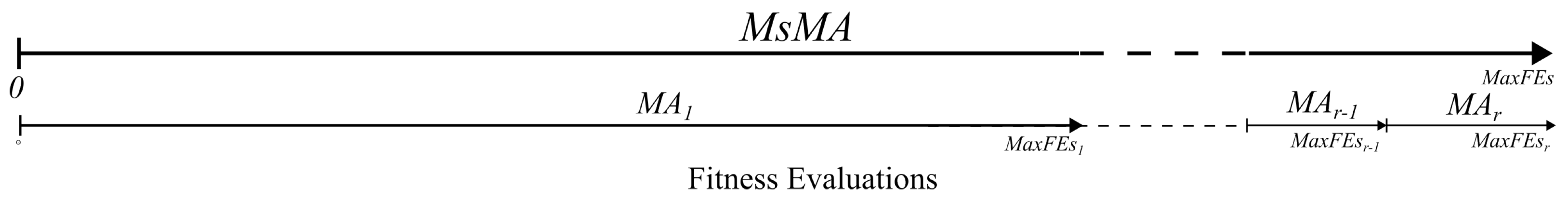
- A novel meta-approach, , for self-adaptive search partitioning based on stagnation detection. It wraps any MA, handling stagnation at the meta-level to enhance efficiency. activates only when stagnation is detected, otherwise allowing the MA to operate unchanged, ensuring broad applicability.
- Demonstration of meta-approach effectiveness by synergizing with . This strategy enhances exploration and exploitation across MAs without modifying their core mechanisms. Applying to showcases improved performance and supports versatile meta-strategy integration.
- Robust evaluation of the proposed approach using the CEC’24 benchmark and the LFA problem. Results show consistent performance improvements over baseline MAs, with novel insights into ABC and CRO behaviors.
2. Related Work
Stagnation
3. Meta-Level Approach to Stagnation
3.1. Leveraging Stagnation for Self-Adapting Search Partitioning
- denotes the expectation (average performance) over multiple optimization runs due to the stochastic nature of the algorithm.
- is a problem-dependent comparison operator, defined as:
MsMA Strategy: Implementation Details
| Algorithm 1. MsMA: A Meta-Level Strategy for Overcoming Stagnation |
|
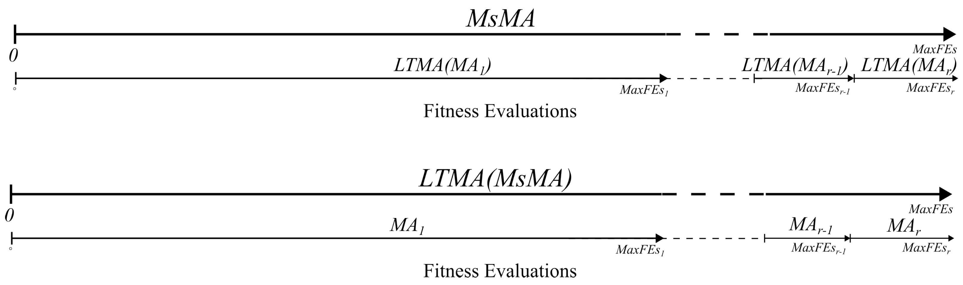
3.2. Synergizing MsMA and LTMA for Improved Performance
| Algorithm 2. LTMA(MsMA): Implementation Variant of MsMA Using LTMA |
|
3.3. Time Complexity Analysis
4. Experiments
4.1. Statistical Analysis
4.2. Benchmark Problems
4.3. MsMA: Meta-Level Strategy Experiment
4.4. LTMA(MsMA): Performance Experiment
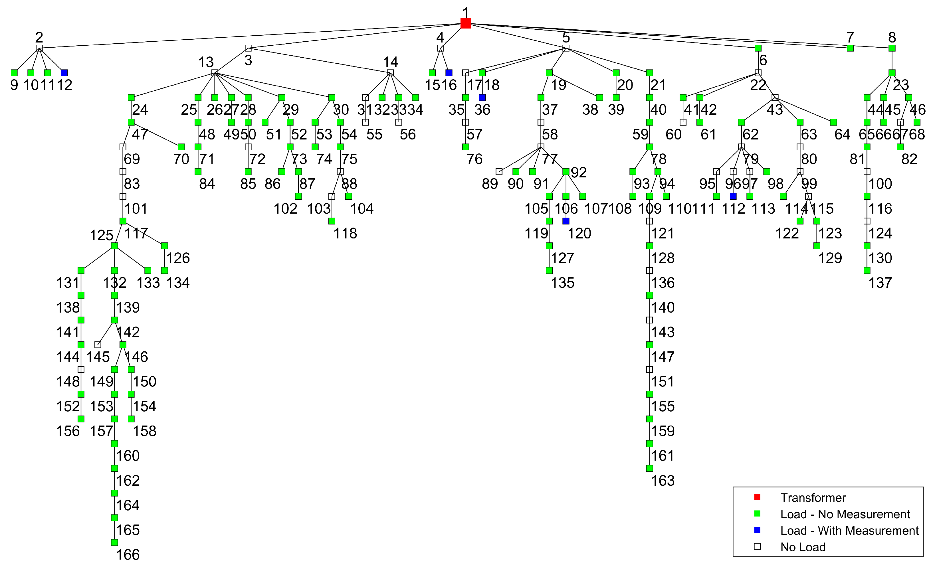
4.5. Experiment: Real-World Optimization Problem
- 1.
- Maximum three-phase active power consumption per consumer (), reflecting realistic load limits (Equation (11)).
- 2.
- Maximum per-phase current, constrained by fuse () ratings to ensure safe operation (Equation (12)).
- 3.
- 4.
- Inductive-only reactive power consumption, preventing unintended reactive power exchange between consumers.
5. Discussion
6. Conclusions
Author Contributions
Funding
Data Availability Statement
Acknowledgments
Conflicts of Interest
Appendix A. Experiment Results
Appendix A.1. Selected CEC’24 Benchmark Problems
Appendix A.2. The MsMA Experiment

| jDE_30 | jDE_6 | jDE_12 | jDE | PSO_30 | PSO_6 | PSO_12 | PSO | MRFO_6 | MRFO_12 | ABC_30 | ABC_12 | ABC_6 | ABC | MRFO_30 | CRO_6 | CRO_12 | MRFO | CRO_30 | CRO | RS | |
|---|---|---|---|---|---|---|---|---|---|---|---|---|---|---|---|---|---|---|---|---|---|
| jDE_30 | 0 | 698 | 188 | 81 | 0 | 1 | 0 | 0 | 3 | 2 | 29 | 29 | 29 | 29 | 2 | 0 | 0 | 1 | 0 | 0 | 0 |
| jDE_6 | 698 | 0 | 192 | 83 | 0 | 1 | 0 | 0 | 2 | 2 | 30 | 30 | 30 | 30 | 3 | 0 | 0 | 1 | 0 | 0 | 0 |
| jDE_12 | 188 | 192 | 0 | 106 | 0 | 0 | 0 | 0 | 2 | 2 | 29 | 29 | 29 | 29 | 3 | 0 | 0 | 2 | 0 | 0 | 0 |
| jDE | 81 | 83 | 106 | 0 | 0 | 0 | 0 | 0 | 0 | 4 | 15 | 15 | 15 | 15 | 2 | 0 | 0 | 2 | 0 | 0 | 0 |
| PSO_30 | 0 | 0 | 0 | 0 | 0 | 29 | 29 | 29 | 24 | 20 | 0 | 0 | 0 | 0 | 19 | 0 | 0 | 11 | 0 | 0 | 0 |
| PSO_6 | 1 | 1 | 0 | 0 | 29 | 0 | 30 | 32 | 26 | 20 | 0 | 0 | 0 | 0 | 20 | 0 | 0 | 11 | 0 | 0 | 0 |
| PSO_12 | 0 | 0 | 0 | 0 | 29 | 30 | 0 | 30 | 25 | 21 | 0 | 0 | 0 | 0 | 18 | 0 | 0 | 11 | 0 | 0 | 0 |
| PSO | 0 | 0 | 0 | 0 | 29 | 32 | 30 | 0 | 24 | 20 | 0 | 0 | 0 | 0 | 18 | 0 | 0 | 11 | 0 | 0 | 0 |
| MRFO_6 | 3 | 2 | 2 | 0 | 24 | 26 | 25 | 24 | 0 | 24 | 0 | 0 | 0 | 0 | 21 | 0 | 0 | 16 | 0 | 0 | 0 |
| MRFO_12 | 2 | 2 | 2 | 4 | 20 | 20 | 21 | 20 | 24 | 0 | 0 | 0 | 0 | 0 | 17 | 0 | 0 | 10 | 0 | 0 | 0 |
| ABC_30 | 29 | 30 | 29 | 15 | 0 | 0 | 0 | 0 | 0 | 0 | 0 | 30 | 30 | 30 | 0 | 0 | 0 | 0 | 0 | 0 | 0 |
| ABC_12 | 29 | 30 | 29 | 15 | 0 | 0 | 0 | 0 | 0 | 0 | 30 | 0 | 30 | 30 | 0 | 0 | 0 | 0 | 0 | 0 | 0 |
| ABC_6 | 29 | 30 | 29 | 15 | 0 | 0 | 0 | 0 | 0 | 0 | 30 | 30 | 0 | 30 | 0 | 0 | 0 | 0 | 0 | 0 | 0 |
| ABC | 29 | 30 | 29 | 15 | 0 | 0 | 0 | 0 | 0 | 0 | 30 | 30 | 30 | 0 | 0 | 0 | 0 | 0 | 0 | 0 | 0 |
| MRFO_30 | 2 | 3 | 3 | 2 | 19 | 20 | 18 | 18 | 21 | 17 | 0 | 0 | 0 | 0 | 0 | 0 | 0 | 7 | 0 | 0 | 0 |
| CRO_6 | 0 | 0 | 0 | 0 | 0 | 0 | 0 | 0 | 0 | 0 | 0 | 0 | 0 | 0 | 0 | 0 | 0 | 0 | 0 | 0 | 0 |
| CRO_12 | 0 | 0 | 0 | 0 | 0 | 0 | 0 | 0 | 0 | 0 | 0 | 0 | 0 | 0 | 0 | 0 | 0 | 0 | 0 | 0 | 0 |
| MRFO | 1 | 1 | 2 | 2 | 11 | 11 | 11 | 11 | 16 | 10 | 0 | 0 | 0 | 0 | 7 | 0 | 0 | 0 | 0 | 0 | 0 |
| CRO_30 | 0 | 0 | 0 | 0 | 0 | 0 | 0 | 0 | 0 | 0 | 0 | 0 | 0 | 0 | 0 | 0 | 0 | 0 | 0 | 0 | 0 |
| CRO | 0 | 0 | 0 | 0 | 0 | 0 | 0 | 0 | 0 | 0 | 0 | 0 | 0 | 0 | 0 | 0 | 0 | 0 | 0 | 0 | 0 |
| RS | 0 | 0 | 0 | 0 | 0 | 0 | 0 | 0 | 0 | 0 | 0 | 0 | 0 | 0 | 0 | 0 | 0 | 0 | 0 | 0 | 0 |
| jDE_30 | jDE_6 | jDE_12 | jDE | PSO_30 | PSO_6 | PSO_12 | PSO | MRFO_6 | MRFO_12 | ABC_30 | ABC_12 | ABC_6 | ABC | MRFO_30 | CRO_6 | CRO_12 | MRFO | CRO_30 | CRO | RS | |
|---|---|---|---|---|---|---|---|---|---|---|---|---|---|---|---|---|---|---|---|---|---|
| jDE_30 | 0 | 138 | 639 | 760 | 867 | 866 | 867 | 867 | 863 | 866 | 825 | 828 | 825 | 827 | 863 | 867 | 868 | 865 | 868 | 869 | 870 |
| jDE_6 | 34 | 0 | 613 | 747 | 847 | 848 | 846 | 848 | 857 | 856 | 823 | 823 | 821 | 824 | 859 | 853 | 858 | 855 | 860 | 858 | 870 |
| jDE_12 | 43 | 65 | 0 | 729 | 861 | 862 | 865 | 867 | 859 | 864 | 823 | 824 | 822 | 826 | 860 | 864 | 868 | 859 | 866 | 868 | 870 |
| jDE | 29 | 40 | 35 | 0 | 863 | 864 | 865 | 864 | 864 | 865 | 824 | 825 | 824 | 825 | 862 | 869 | 868 | 865 | 869 | 869 | 870 |
| PSO_30 | 3 | 23 | 9 | 7 | 0 | 426 | 421 | 420 | 550 | 569 | 533 | 532 | 533 | 532 | 583 | 611 | 633 | 642 | 668 | 672 | 870 |
| PSO_6 | 3 | 21 | 8 | 6 | 415 | 0 | 403 | 419 | 554 | 563 | 525 | 511 | 527 | 534 | 602 | 596 | 626 | 635 | 670 | 694 | 868 |
| PSO_12 | 3 | 24 | 5 | 5 | 420 | 437 | 0 | 443 | 549 | 561 | 524 | 514 | 513 | 533 | 597 | 583 | 618 | 629 | 677 | 674 | 870 |
| PSO | 3 | 22 | 3 | 6 | 421 | 419 | 397 | 0 | 559 | 553 | 522 | 517 | 513 | 524 | 581 | 601 | 616 | 622 | 655 | 674 | 870 |
| MRFO_6 | 4 | 11 | 9 | 6 | 296 | 290 | 296 | 287 | 0 | 436 | 481 | 477 | 486 | 494 | 477 | 477 | 502 | 540 | 544 | 589 | 869 |
| MRFO_12 | 2 | 12 | 4 | 1 | 281 | 287 | 288 | 297 | 410 | 0 | 477 | 466 | 464 | 471 | 454 | 452 | 481 | 513 | 545 | 550 | 868 |
| ABC_30 | 16 | 17 | 18 | 31 | 337 | 345 | 346 | 348 | 389 | 393 | 0 | 446 | 437 | 426 | 438 | 434 | 480 | 484 | 517 | 533 | 855 |
| ABC_12 | 13 | 17 | 17 | 30 | 338 | 359 | 356 | 353 | 393 | 404 | 394 | 0 | 423 | 400 | 434 | 436 | 476 | 493 | 526 | 550 | 857 |
| ABC_6 | 16 | 19 | 19 | 31 | 337 | 343 | 357 | 357 | 384 | 406 | 403 | 417 | 0 | 412 | 434 | 456 | 471 | 476 | 513 | 545 | 856 |
| ABC | 14 | 16 | 15 | 30 | 338 | 336 | 337 | 346 | 376 | 399 | 414 | 440 | 428 | 0 | 440 | 437 | 468 | 490 | 511 | 549 | 848 |
| MRFO_30 | 5 | 8 | 7 | 6 | 268 | 248 | 255 | 271 | 372 | 399 | 432 | 436 | 436 | 430 | 0 | 440 | 460 | 506 | 528 | 549 | 869 |
| CRO_6 | 3 | 17 | 6 | 1 | 259 | 274 | 287 | 269 | 393 | 418 | 436 | 434 | 414 | 433 | 430 | 0 | 457 | 512 | 522 | 511 | 868 |
| CRO_12 | 2 | 12 | 2 | 2 | 237 | 244 | 252 | 254 | 368 | 389 | 390 | 394 | 399 | 402 | 410 | 413 | 0 | 475 | 478 | 516 | 863 |
| MRFO | 4 | 14 | 9 | 3 | 217 | 224 | 230 | 237 | 314 | 347 | 386 | 377 | 394 | 380 | 357 | 358 | 395 | 0 | 454 | 463 | 869 |
| CRO_30 | 2 | 10 | 4 | 1 | 202 | 200 | 193 | 215 | 326 | 325 | 353 | 344 | 357 | 359 | 342 | 348 | 392 | 416 | 0 | 451 | 862 |
| CRO | 1 | 12 | 2 | 1 | 198 | 176 | 196 | 196 | 281 | 320 | 337 | 320 | 325 | 321 | 321 | 359 | 354 | 407 | 419 | 0 | 856 |
| RS | 0 | 0 | 0 | 0 | 0 | 2 | 0 | 0 | 1 | 2 | 15 | 13 | 14 | 22 | 1 | 2 | 7 | 1 | 8 | 14 | 0 |
| F01 | F02 | F03 | F04 | F05 | F06 | F07 | F08 | F09 | F10 | F11 | F12 | F13 | F14 | F15 | |
|---|---|---|---|---|---|---|---|---|---|---|---|---|---|---|---|
| jDE_30 | 510 | 510 | 460 | 567 | 405 | 569 | 569 | 569 | 569 | 569 | 569 | 569 | 569 | 569 | 569 |
| jDE_6 | 510 | 510 | 437 | 352 | 407 | 566 | 566 | 566 | 566 | 566 | 566 | 566 | 566 | 566 | 566 |
| jDE_12 | 510 | 510 | 424 | 531 | 406 | 541 | 541 | 541 | 541 | 541 | 541 | 541 | 541 | 541 | 541 |
| jDE | 510 | 510 | 448 | 561 | 390 | 510 | 510 | 510 | 510 | 510 | 510 | 510 | 510 | 510 | 510 |
| PSO_30 | 294 | 267 | 256 | 406 | 237 | 295 | 378 | 404 | 248 | 408 | 372 | 359 | 370 | 388 | 318 |
| PSO_6 | 276 | 146 | 228 | 373 | 165 | 247 | 363 | 404 | 263 | 412 | 374 | 391 | 396 | 426 | 356 |
| PSO_12 | 273 | 179 | 228 | 410 | 207 | 253 | 397 | 428 | 272 | 406 | 358 | 392 | 387 | 362 | 291 |
| PSO | 284 | 325 | 211 | 385 | 207 | 274 | 361 | 403 | 260 | 408 | 358 | 381 | 384 | 386 | 298 |
| MRFO_6 | 330 | 224 | 290 | 236 | 83 | 211 | 289 | 262 | 119 | 311 | 362 | 275 | 355 | 266 | 261 |
| MRFO_12 | 304 | 311 | 254 | 268 | 80 | 197 | 295 | 220 | 135 | 292 | 388 | 277 | 349 | 274 | 275 |
| ABC_30 | 366 | 75 | 464 | 132 | 407 | 295 | 119 | 82 | 377 | 80 | 157 | 136 | 146 | 165 | 287 |
| ABC_12 | 363 | 65 | 439 | 182 | 407 | 293 | 109 | 67 | 369 | 88 | 136 | 102 | 151 | 136 | 302 |
| ABC_6 | 359 | 77 | 468 | 137 | 407 | 287 | 115 | 96 | 374 | 91 | 162 | 78 | 160 | 104 | 332 |
| ABC | 381 | 39 | 433 | 125 | 407 | 300 | 133 | 103 | 363 | 60 | 165 | 167 | 130 | 172 | 313 |
| MRFO_30 | 220 | 462 | 335 | 196 | 72 | 241 | 267 | 266 | 69 | 261 | 398 | 169 | 356 | 188 | 226 |
| CRO_6 | 112 | 267 | 181 | 366 | 263 | 323 | 304 | 315 | 345 | 245 | 117 | 325 | 141 | 323 | 202 |
| CRO_12 | 112 | 346 | 150 | 294 | 298 | 308 | 261 | 288 | 254 | 247 | 131 | 316 | 131 | 299 | 179 |
| MRFO | 141 | 464 | 308 | 200 | 68 | 153 | 230 | 233 | 125 | 270 | 387 | 165 | 379 | 160 | 168 |
| CRO_30 | 124 | 384 | 112 | 293 | 332 | 206 | 244 | 269 | 261 | 258 | 106 | 296 | 116 | 243 | 129 |
| CRO | 141 | 391 | 91 | 286 | 328 | 197 | 215 | 240 | 246 | 243 | 109 | 251 | 98 | 188 | 143 |
| RS | 0 | 58 | 0 | 0 | 0 | 0 | 0 | 0 | 0 | 0 | 0 | 0 | 31 | 0 | 0 |
| F16 | F17 | F18 | F19 | F20 | F21 | F22 | F23 | F24 | F25 | F26 | F27 | F28 | F29 | |
|---|---|---|---|---|---|---|---|---|---|---|---|---|---|---|
| jDE_30 | 569 | 569 | 569 | 569 | 569 | 569 | 569 | 569 | 569 | 569 | 569 | 569 | 569 | 569 |
| jDE_6 | 566 | 566 | 566 | 566 | 566 | 566 | 566 | 566 | 566 | 566 | 566 | 566 | 566 | 566 |
| jDE_12 | 541 | 541 | 541 | 541 | 541 | 541 | 541 | 541 | 541 | 541 | 541 | 541 | 541 | 541 |
| jDE | 510 | 510 | 510 | 510 | 510 | 510 | 510 | 510 | 510 | 510 | 510 | 510 | 510 | 510 |
| PSO_30 | 321 | 398 | 331 | 231 | 269 | 315 | 300 | 300 | 287 | 308 | 271 | 240 | 276 | 390 |
| PSO_6 | 308 | 390 | 406 | 258 | 297 | 318 | 314 | 299 | 272 | 282 | 312 | 222 | 303 | 379 |
| PSO_12 | 331 | 377 | 374 | 276 | 301 | 318 | 291 | 289 | 272 | 307 | 292 | 270 | 257 | 381 |
| PSO | 290 | 396 | 362 | 245 | 275 | 318 | 327 | 280 | 260 | 284 | 236 | 247 | 264 | 369 |
| MRFO_6 | 210 | 244 | 329 | 289 | 273 | 264 | 215 | 229 | 331 | 224 | 230 | 343 | 163 | 353 |
| MRFO_12 | 217 | 226 | 304 | 286 | 206 | 230 | 165 | 259 | 370 | 215 | 175 | 284 | 184 | 283 |
| ABC_30 | 322 | 220 | 100 | 313 | 339 | 132 | 358 | 260 | 347 | 389 | 390 | 338 | 375 | 119 |
| ABC_12 | 330 | 186 | 120 | 314 | 363 | 137 | 384 | 339 | 332 | 393 | 389 | 340 | 355 | 78 |
| ABC_6 | 317 | 212 | 71 | 337 | 322 | 147 | 317 | 404 | 329 | 405 | 401 | 321 | 361 | 61 |
| ABC | 311 | 201 | 119 | 329 | 322 | 138 | 298 | 275 | 358 | 370 | 410 | 366 | 359 | 85 |
| MRFO_30 | 187 | 271 | 322 | 217 | 220 | 223 | 152 | 197 | 292 | 231 | 156 | 270 | 173 | 288 |
| CRO_6 | 237 | 197 | 298 | 284 | 216 | 232 | 237 | 248 | 128 | 178 | 195 | 108 | 286 | 271 |
| CRO_12 | 254 | 190 | 304 | 222 | 172 | 201 | 205 | 233 | 150 | 164 | 176 | 133 | 203 | 281 |
| MRFO | 171 | 276 | 206 | 238 | 180 | 193 | 106 | 137 | 157 | 100 | 104 | 285 | 157 | 271 |
| CRO_30 | 140 | 134 | 199 | 138 | 174 | 198 | 213 | 177 | 85 | 103 | 187 | 167 | 202 | 212 |
| CRO | 134 | 160 | 235 | 96 | 151 | 181 | 198 | 154 | 110 | 119 | 156 | 120 | 162 | 259 |
| RS | 0 | 2 | 0 | 7 | 0 | 4 | 0 | 0 | 0 | 0 | 0 | 0 | 0 | 0 |
| F01 | F02 | F03 | F04 | F05 | F06 | F07 | F08 | F09 | F10 | F11 | F12 | F13 | F14 | F15 | |
|---|---|---|---|---|---|---|---|---|---|---|---|---|---|---|---|
| jDE_30 | 90 | 90 | 27 | 0 | 189 | 29 | 29 | 29 | 29 | 29 | 29 | 29 | 29 | 29 | 29 |
| jDE_6 | 90 | 90 | 33 | 0 | 193 | 29 | 29 | 29 | 29 | 29 | 29 | 29 | 29 | 29 | 29 |
| jDE_12 | 90 | 90 | 27 | 0 | 188 | 9 | 9 | 9 | 9 | 9 | 9 | 9 | 9 | 9 | 9 |
| jDE | 90 | 90 | 28 | 0 | 106 | 1 | 1 | 1 | 1 | 1 | 1 | 1 | 1 | 1 | 1 |
| PSO_30 | 0 | 0 | 0 | 0 | 0 | 0 | 0 | 0 | 0 | 0 | 0 | 0 | 0 | 0 | 0 |
| PSO_6 | 0 | 0 | 3 | 0 | 0 | 0 | 0 | 0 | 0 | 0 | 0 | 0 | 0 | 0 | 0 |
| PSO_12 | 0 | 0 | 2 | 0 | 0 | 0 | 0 | 0 | 0 | 0 | 0 | 0 | 0 | 0 | 0 |
| PSO | 0 | 0 | 0 | 0 | 0 | 0 | 0 | 0 | 0 | 0 | 0 | 0 | 0 | 0 | 0 |
| MRFO_6 | 0 | 0 | 12 | 0 | 0 | 0 | 0 | 0 | 0 | 0 | 0 | 0 | 0 | 0 | 0 |
| MRFO_12 | 0 | 0 | 15 | 0 | 0 | 0 | 0 | 0 | 0 | 0 | 0 | 0 | 0 | 0 | 0 |
| ABC_30 | 0 | 0 | 0 | 0 | 193 | 0 | 0 | 0 | 0 | 0 | 0 | 0 | 0 | 0 | 0 |
| ABC_12 | 0 | 0 | 0 | 0 | 193 | 0 | 0 | 0 | 0 | 0 | 0 | 0 | 0 | 0 | 0 |
| ABC_6 | 0 | 0 | 0 | 0 | 193 | 0 | 0 | 0 | 0 | 0 | 0 | 0 | 0 | 0 | 0 |
| ABC | 0 | 0 | 0 | 0 | 193 | 0 | 0 | 0 | 0 | 0 | 0 | 0 | 0 | 0 | 0 |
| MRFO_30 | 0 | 0 | 11 | 0 | 0 | 0 | 0 | 0 | 0 | 0 | 0 | 0 | 0 | 0 | 0 |
| CRO_6 | 0 | 0 | 0 | 0 | 0 | 0 | 0 | 0 | 0 | 0 | 0 | 0 | 0 | 0 | 0 |
| CRO_12 | 0 | 0 | 0 | 0 | 0 | 0 | 0 | 0 | 0 | 0 | 0 | 0 | 0 | 0 | 0 |
| MRFO | 0 | 0 | 8 | 0 | 0 | 0 | 0 | 0 | 0 | 0 | 0 | 0 | 0 | 0 | 0 |
| CRO_30 | 0 | 0 | 0 | 0 | 0 | 0 | 0 | 0 | 0 | 0 | 0 | 0 | 0 | 0 | 0 |
| CRO | 0 | 0 | 0 | 0 | 0 | 0 | 0 | 0 | 0 | 0 | 0 | 0 | 0 | 0 | 0 |
| RS | 0 | 0 | 0 | 0 | 0 | 0 | 0 | 0 | 0 | 0 | 0 | 0 | 0 | 0 | 0 |
| F16 | F17 | F18 | F19 | F20 | F21 | F22 | F23 | F24 | F25 | F26 | F27 | F28 | F29 | |
|---|---|---|---|---|---|---|---|---|---|---|---|---|---|---|
| jDE_30 | 29 | 29 | 29 | 29 | 29 | 29 | 29 | 29 | 29 | 29 | 29 | 29 | 29 | 29 |
| jDE_6 | 29 | 29 | 29 | 29 | 29 | 29 | 29 | 29 | 29 | 29 | 29 | 29 | 29 | 29 |
| jDE_12 | 9 | 9 | 9 | 9 | 9 | 9 | 9 | 9 | 9 | 9 | 9 | 9 | 9 | 9 |
| jDE | 1 | 1 | 1 | 1 | 1 | 1 | 1 | 1 | 1 | 1 | 1 | 1 | 1 | 1 |
| PSO_30 | 0 | 0 | 0 | 0 | 0 | 159 | 0 | 0 | 0 | 2 | 0 | 0 | 0 | 0 |
| PSO_6 | 0 | 0 | 0 | 0 | 0 | 162 | 0 | 0 | 0 | 5 | 0 | 0 | 0 | 0 |
| PSO_12 | 0 | 0 | 0 | 0 | 0 | 162 | 0 | 0 | 0 | 0 | 0 | 0 | 0 | 0 |
| PSO | 0 | 0 | 0 | 0 | 0 | 162 | 0 | 0 | 0 | 2 | 0 | 0 | 0 | 0 |
| MRFO_6 | 0 | 0 | 0 | 0 | 0 | 136 | 0 | 0 | 0 | 2 | 0 | 17 | 0 | 0 |
| MRFO_12 | 0 | 0 | 0 | 0 | 0 | 114 | 0 | 0 | 0 | 0 | 0 | 13 | 0 | 0 |
| ABC_30 | 0 | 0 | 0 | 0 | 0 | 0 | 0 | 0 | 0 | 0 | 0 | 0 | 0 | 0 |
| ABC_12 | 0 | 0 | 0 | 0 | 0 | 0 | 0 | 0 | 0 | 0 | 0 | 0 | 0 | 0 |
| ABC_6 | 0 | 0 | 0 | 0 | 0 | 0 | 0 | 0 | 0 | 0 | 0 | 0 | 0 | 0 |
| ABC | 0 | 0 | 0 | 0 | 0 | 0 | 0 | 0 | 0 | 0 | 0 | 0 | 0 | 0 |
| MRFO_30 | 0 | 0 | 0 | 0 | 0 | 105 | 0 | 0 | 0 | 5 | 0 | 9 | 0 | 0 |
| CRO_6 | 0 | 0 | 0 | 0 | 0 | 0 | 0 | 0 | 0 | 0 | 0 | 0 | 0 | 0 |
| CRO_12 | 0 | 0 | 0 | 0 | 0 | 0 | 0 | 0 | 0 | 0 | 0 | 0 | 0 | 0 |
| MRFO | 0 | 0 | 0 | 0 | 0 | 62 | 0 | 0 | 0 | 0 | 0 | 13 | 0 | 0 |
| CRO_30 | 0 | 0 | 0 | 0 | 0 | 0 | 0 | 0 | 0 | 0 | 0 | 0 | 0 | 0 |
| CRO | 0 | 0 | 0 | 0 | 0 | 0 | 0 | 0 | 0 | 0 | 0 | 0 | 0 | 0 |
| RS | 0 | 0 | 0 | 0 | 0 | 0 | 0 | 0 | 0 | 0 | 0 | 0 | 0 | 0 |
Appendix A.3. The LTMA(MsMA) Experiment
| jDE_30 | jDE_LTMA_30 | jDE_LTMA_6 | jDE_LTMA_12 | jDE | PSO_LTMA_6 | PSO_LTMA_12 | PSO_LTMA_30 | PSO_30 | PSO | CRO_LTMA_12 | MRFO_LTMA_6 | CRO_LTMA_6 | MRFO_6 | ABC_LTMA_12 | ABC_LTMA_30 | MRFO_LTMA_30 | ABC_30 | ABC | MRFO_LTMA_12 | ABC_LTMA_6 | CRO_LTMA_30 | CRO_6 | MRFO | CRO | RS | |
|---|---|---|---|---|---|---|---|---|---|---|---|---|---|---|---|---|---|---|---|---|---|---|---|---|---|---|
| jDE_30 | 0 | 349 | 55 | 402 | 760 | 867 | 867 | 865 | 867 | 867 | 866 | 864 | 867 | 863 | 825 | 828 | 863 | 825 | 827 | 861 | 827 | 868 | 867 | 865 | 869 | 870 |
| jDE_LTMA_30 | 404 | 0 | 434 | 422 | 750 | 863 | 866 | 860 | 863 | 863 | 863 | 862 | 862 | 863 | 822 | 825 | 863 | 822 | 823 | 860 | 825 | 865 | 864 | 861 | 867 | 870 |
| jDE_LTMA_6 | 36 | 348 | 0 | 372 | 746 | 838 | 840 | 841 | 841 | 842 | 840 | 841 | 840 | 846 | 816 | 818 | 846 | 814 | 823 | 844 | 815 | 841 | 841 | 850 | 849 | 870 |
| jDE_LTMA_12 | 39 | 354 | 74 | 0 | 747 | 851 | 853 | 853 | 851 | 854 | 851 | 855 | 850 | 858 | 822 | 825 | 859 | 822 | 823 | 859 | 823 | 858 | 857 | 859 | 860 | 870 |
| jDE | 29 | 36 | 51 | 39 | 0 | 865 | 868 | 864 | 863 | 864 | 866 | 864 | 867 | 864 | 825 | 825 | 862 | 824 | 825 | 862 | 825 | 869 | 869 | 865 | 869 | 870 |
| PSO_LTMA_6 | 3 | 7 | 32 | 19 | 5 | 0 | 442 | 462 | 455 | 485 | 600 | 598 | 607 | 598 | 583 | 576 | 624 | 575 | 574 | 603 | 581 | 635 | 650 | 653 | 721 | 869 |
| PSO_LTMA_12 | 3 | 4 | 30 | 17 | 1 | 397 | 0 | 437 | 447 | 472 | 575 | 563 | 605 | 585 | 550 | 562 | 592 | 559 | 555 | 597 | 565 | 620 | 636 | 653 | 710 | 869 |
| PSO_LTMA_30 | 5 | 9 | 29 | 17 | 6 | 378 | 403 | 0 | 410 | 420 | 574 | 558 | 578 | 554 | 529 | 528 | 560 | 539 | 538 | 574 | 544 | 595 | 611 | 630 | 679 | 870 |
| PSO_30 | 3 | 7 | 29 | 19 | 7 | 386 | 394 | 430 | 0 | 420 | 567 | 551 | 574 | 550 | 518 | 540 | 563 | 533 | 532 | 556 | 545 | 590 | 611 | 642 | 672 | 870 |
| PSO | 3 | 7 | 28 | 16 | 6 | 355 | 368 | 418 | 421 | 0 | 572 | 560 | 551 | 559 | 519 | 520 | 557 | 522 | 524 | 578 | 540 | 590 | 601 | 622 | 674 | 870 |
| CRO_LTMA_12 | 4 | 7 | 30 | 19 | 4 | 270 | 295 | 296 | 303 | 298 | 0 | 423 | 501 | 460 | 468 | 484 | 488 | 491 | 488 | 466 | 476 | 473 | 481 | 538 | 584 | 870 |
| MRFO_LTMA_6 | 5 | 7 | 27 | 13 | 5 | 246 | 280 | 286 | 293 | 283 | 447 | 0 | 438 | 422 | 506 | 501 | 447 | 489 | 514 | 433 | 503 | 471 | 493 | 536 | 570 | 870 |
| CRO_LTMA_6 | 3 | 8 | 30 | 20 | 3 | 263 | 265 | 292 | 296 | 319 | 369 | 432 | 0 | 445 | 496 | 502 | 479 | 509 | 505 | 465 | 500 | 454 | 463 | 534 | 580 | 868 |
| MRFO_6 | 4 | 5 | 22 | 9 | 6 | 248 | 260 | 291 | 296 | 287 | 410 | 415 | 425 | 0 | 477 | 486 | 452 | 481 | 494 | 436 | 480 | 471 | 477 | 540 | 589 | 869 |
| ABC_LTMA_12 | 16 | 19 | 24 | 18 | 30 | 287 | 320 | 341 | 352 | 351 | 402 | 364 | 374 | 393 | 0 | 408 | 394 | 418 | 399 | 414 | 454 | 461 | 454 | 478 | 560 | 853 |
| ABC_LTMA_30 | 13 | 16 | 22 | 15 | 30 | 294 | 308 | 342 | 330 | 350 | 386 | 369 | 368 | 384 | 432 | 0 | 407 | 430 | 427 | 412 | 467 | 457 | 435 | 487 | 544 | 853 |
| MRFO_LTMA_30 | 4 | 5 | 22 | 8 | 3 | 227 | 259 | 290 | 288 | 294 | 382 | 397 | 391 | 393 | 476 | 463 | 0 | 476 | 469 | 419 | 482 | 448 | 456 | 504 | 550 | 868 |
| ABC_30 | 16 | 19 | 26 | 18 | 31 | 295 | 311 | 331 | 337 | 348 | 379 | 381 | 361 | 389 | 422 | 410 | 394 | 0 | 426 | 413 | 460 | 457 | 434 | 484 | 533 | 855 |
| ABC | 14 | 18 | 17 | 17 | 30 | 296 | 315 | 332 | 338 | 346 | 382 | 356 | 365 | 376 | 441 | 413 | 401 | 414 | 0 | 413 | 465 | 452 | 437 | 490 | 549 | 848 |
| MRFO_LTMA_12 | 5 | 5 | 22 | 8 | 5 | 243 | 249 | 273 | 292 | 269 | 404 | 411 | 405 | 407 | 456 | 458 | 434 | 457 | 457 | 0 | 460 | 440 | 454 | 505 | 545 | 870 |
| ABC_LTMA_6 | 14 | 16 | 25 | 17 | 30 | 289 | 305 | 326 | 325 | 330 | 394 | 367 | 370 | 390 | 386 | 373 | 388 | 380 | 375 | 410 | 0 | 449 | 434 | 468 | 528 | 859 |
| CRO_LTMA_30 | 2 | 5 | 29 | 12 | 1 | 235 | 250 | 275 | 280 | 280 | 397 | 399 | 416 | 399 | 409 | 413 | 422 | 413 | 418 | 430 | 421 | 0 | 452 | 501 | 547 | 863 |
| CRO_6 | 3 | 6 | 29 | 13 | 1 | 220 | 234 | 259 | 259 | 269 | 389 | 377 | 407 | 393 | 416 | 435 | 414 | 436 | 433 | 416 | 436 | 418 | 0 | 512 | 511 | 868 |
| MRFO | 4 | 5 | 19 | 10 | 3 | 206 | 206 | 228 | 217 | 237 | 332 | 317 | 336 | 314 | 392 | 383 | 355 | 386 | 380 | 353 | 402 | 369 | 358 | 0 | 463 | 869 |
| CRO | 1 | 3 | 21 | 10 | 1 | 149 | 160 | 191 | 198 | 196 | 286 | 300 | 290 | 281 | 310 | 326 | 320 | 337 | 321 | 325 | 342 | 323 | 359 | 407 | 0 | 856 |
| RS | 0 | 0 | 0 | 0 | 0 | 1 | 1 | 0 | 0 | 0 | 0 | 0 | 2 | 1 | 17 | 17 | 2 | 15 | 22 | 0 | 11 | 7 | 2 | 1 | 14 | 0 |
| jDE_30 | jDE_LTMA_30 | jDE_LTMA_6 | jDE_LTMA_12 | jDE | PSO_LTMA_6 | PSO_LTMA_12 | PSO_LTMA_30 | PSO_30 | PSO | CRO_LTMA_12 | MRFO_LTMA_6 | CRO_LTMA_6 | MRFO_6 | ABC_LTMA_12 | ABC_LTMA_30 | MRFO_LTMA_30 | ABC_30 | ABC | MRFO_LTMA_12 | ABC_LTMA_6 | CRO_LTMA_30 | CRO_6 | MRFO | CRO | RS | |
|---|---|---|---|---|---|---|---|---|---|---|---|---|---|---|---|---|---|---|---|---|---|---|---|---|---|---|
| jDE_30 | 0 | 117 | 779 | 429 | 81 | 0 | 0 | 0 | 0 | 0 | 0 | 1 | 0 | 3 | 29 | 29 | 3 | 29 | 29 | 4 | 29 | 0 | 0 | 1 | 0 | 0 |
| jDE_LTMA_30 | 117 | 0 | 88 | 94 | 84 | 0 | 0 | 1 | 0 | 0 | 0 | 1 | 0 | 2 | 29 | 29 | 2 | 29 | 29 | 5 | 29 | 0 | 0 | 4 | 0 | 0 |
| jDE_LTMA_6 | 779 | 88 | 0 | 424 | 73 | 0 | 0 | 0 | 0 | 0 | 0 | 2 | 0 | 2 | 30 | 30 | 2 | 30 | 30 | 4 | 30 | 0 | 0 | 1 | 0 | 0 |
| jDE_LTMA_12 | 429 | 94 | 424 | 0 | 84 | 0 | 0 | 0 | 0 | 0 | 0 | 2 | 0 | 3 | 30 | 30 | 3 | 30 | 30 | 3 | 30 | 0 | 0 | 1 | 0 | 0 |
| jDE | 81 | 84 | 73 | 84 | 0 | 0 | 1 | 0 | 0 | 0 | 0 | 1 | 0 | 0 | 15 | 15 | 5 | 15 | 15 | 3 | 15 | 0 | 0 | 2 | 0 | 0 |
| PSO_LTMA_6 | 0 | 0 | 0 | 0 | 0 | 0 | 31 | 30 | 29 | 30 | 0 | 26 | 0 | 24 | 0 | 0 | 19 | 0 | 0 | 24 | 0 | 0 | 0 | 11 | 0 | 0 |
| PSO_LTMA_12 | 0 | 0 | 0 | 0 | 1 | 31 | 0 | 30 | 29 | 30 | 0 | 27 | 0 | 25 | 0 | 0 | 19 | 0 | 0 | 24 | 0 | 0 | 0 | 11 | 0 | 0 |
| PSO_LTMA_30 | 0 | 1 | 0 | 0 | 0 | 30 | 30 | 0 | 30 | 32 | 0 | 26 | 0 | 25 | 0 | 0 | 20 | 0 | 0 | 23 | 0 | 0 | 0 | 12 | 0 | 0 |
| PSO_30 | 0 | 0 | 0 | 0 | 0 | 29 | 29 | 30 | 0 | 29 | 0 | 26 | 0 | 24 | 0 | 0 | 19 | 0 | 0 | 22 | 0 | 0 | 0 | 11 | 0 | 0 |
| PSO | 0 | 0 | 0 | 0 | 0 | 30 | 30 | 32 | 29 | 0 | 0 | 27 | 0 | 24 | 0 | 0 | 19 | 0 | 0 | 23 | 0 | 0 | 0 | 11 | 0 | 0 |
| CRO_LTMA_12 | 0 | 0 | 0 | 0 | 0 | 0 | 0 | 0 | 0 | 0 | 0 | 0 | 0 | 0 | 0 | 0 | 0 | 0 | 0 | 0 | 0 | 0 | 0 | 0 | 0 | 0 |
| MRFO_LTMA_6 | 1 | 1 | 2 | 2 | 1 | 26 | 27 | 26 | 26 | 27 | 0 | 0 | 0 | 33 | 0 | 0 | 26 | 0 | 0 | 26 | 0 | 0 | 0 | 17 | 0 | 0 |
| CRO_LTMA_6 | 0 | 0 | 0 | 0 | 0 | 0 | 0 | 0 | 0 | 0 | 0 | 0 | 0 | 0 | 0 | 0 | 0 | 0 | 0 | 0 | 0 | 0 | 0 | 0 | 0 | 0 |
| MRFO_6 | 3 | 2 | 2 | 3 | 0 | 24 | 25 | 25 | 24 | 24 | 0 | 33 | 0 | 0 | 0 | 0 | 25 | 0 | 0 | 27 | 0 | 0 | 0 | 16 | 0 | 0 |
| ABC_LTMA_12 | 29 | 29 | 30 | 30 | 15 | 0 | 0 | 0 | 0 | 0 | 0 | 0 | 0 | 0 | 0 | 30 | 0 | 30 | 30 | 0 | 30 | 0 | 0 | 0 | 0 | 0 |
| ABC_LTMA_30 | 29 | 29 | 30 | 30 | 15 | 0 | 0 | 0 | 0 | 0 | 0 | 0 | 0 | 0 | 30 | 0 | 0 | 30 | 30 | 0 | 30 | 0 | 0 | 0 | 0 | 0 |
| MRFO_LTMA_30 | 3 | 2 | 2 | 3 | 5 | 19 | 19 | 20 | 19 | 19 | 0 | 26 | 0 | 25 | 0 | 0 | 0 | 0 | 0 | 17 | 0 | 0 | 0 | 11 | 0 | 0 |
| ABC_30 | 29 | 29 | 30 | 30 | 15 | 0 | 0 | 0 | 0 | 0 | 0 | 0 | 0 | 0 | 30 | 30 | 0 | 0 | 30 | 0 | 30 | 0 | 0 | 0 | 0 | 0 |
| ABC | 29 | 29 | 30 | 30 | 15 | 0 | 0 | 0 | 0 | 0 | 0 | 0 | 0 | 0 | 30 | 30 | 0 | 30 | 0 | 0 | 30 | 0 | 0 | 0 | 0 | 0 |
| MRFO_LTMA_12 | 4 | 5 | 4 | 3 | 3 | 24 | 24 | 23 | 22 | 23 | 0 | 26 | 0 | 27 | 0 | 0 | 17 | 0 | 0 | 0 | 0 | 0 | 0 | 12 | 0 | 0 |
| ABC_LTMA_6 | 29 | 29 | 30 | 30 | 15 | 0 | 0 | 0 | 0 | 0 | 0 | 0 | 0 | 0 | 30 | 30 | 0 | 30 | 30 | 0 | 0 | 0 | 0 | 0 | 0 | 0 |
| CRO_LTMA_30 | 0 | 0 | 0 | 0 | 0 | 0 | 0 | 0 | 0 | 0 | 0 | 0 | 0 | 0 | 0 | 0 | 0 | 0 | 0 | 0 | 0 | 0 | 0 | 0 | 0 | 0 |
| CRO_6 | 0 | 0 | 0 | 0 | 0 | 0 | 0 | 0 | 0 | 0 | 0 | 0 | 0 | 0 | 0 | 0 | 0 | 0 | 0 | 0 | 0 | 0 | 0 | 0 | 0 | 0 |
| MRFO | 1 | 4 | 1 | 1 | 2 | 11 | 11 | 12 | 11 | 11 | 0 | 17 | 0 | 16 | 0 | 0 | 11 | 0 | 0 | 12 | 0 | 0 | 0 | 0 | 0 | 0 |
| CRO | 0 | 0 | 0 | 0 | 0 | 0 | 0 | 0 | 0 | 0 | 0 | 0 | 0 | 0 | 0 | 0 | 0 | 0 | 0 | 0 | 0 | 0 | 0 | 0 | 0 | 0 |
| RS | 0 | 0 | 0 | 0 | 0 | 0 | 0 | 0 | 0 | 0 | 0 | 0 | 0 | 0 | 0 | 0 | 0 | 0 | 0 | 0 | 0 | 0 | 0 | 0 | 0 | 0 |
| F01 | F02 | F03 | F04 | F05 | F06 | F07 | F08 | F09 | F10 | F11 | F12 | F13 | F14 | F15 | |
|---|---|---|---|---|---|---|---|---|---|---|---|---|---|---|---|
| jDE_30 | 630 | 639 | 574 | 704 | 495 | 688 | 688 | 688 | 688 | 688 | 688 | 688 | 688 | 688 | 688 |
| jDE_LTMA_30 | 630 | 639 | 537 | 648 | 496 | 708 | 708 | 708 | 708 | 708 | 708 | 708 | 708 | 708 | 708 |
| jDE_LTMA_6 | 630 | 630 | 555 | 226 | 497 | 690 | 690 | 690 | 690 | 690 | 690 | 690 | 690 | 690 | 690 |
| jDE_LTMA_12 | 630 | 639 | 535 | 502 | 497 | 676 | 676 | 676 | 676 | 676 | 676 | 676 | 676 | 676 | 676 |
| jDE | 630 | 639 | 553 | 707 | 481 | 630 | 630 | 630 | 630 | 630 | 630 | 630 | 630 | 630 | 630 |
| PSO_LTMA_6 | 377 | 194 | 278 | 534 | 216 | 292 | 473 | 476 | 309 | 509 | 408 | 529 | 479 | 526 | 485 |
| PSO_LTMA_12 | 381 | 225 | 300 | 474 | 278 | 312 | 433 | 527 | 303 | 514 | 433 | 474 | 466 | 508 | 442 |
| PSO_LTMA_30 | 337 | 342 | 313 | 492 | 301 | 298 | 404 | 509 | 314 | 504 | 474 | 458 | 476 | 466 | 386 |
| PSO_30 | 367 | 403 | 306 | 483 | 328 | 330 | 433 | 501 | 282 | 517 | 469 | 440 | 450 | 475 | 339 |
| PSO | 355 | 485 | 273 | 461 | 293 | 301 | 432 | 504 | 298 | 517 | 451 | 452 | 472 | 464 | 328 |
| CRO_LTMA_12 | 60 | 290 | 185 | 538 | 300 | 477 | 432 | 383 | 442 | 311 | 189 | 446 | 237 | 387 | 348 |
| MRFO_LTMA_6 | 358 | 340 | 367 | 340 | 80 | 313 | 311 | 284 | 114 | 374 | 466 | 299 | 434 | 350 | 353 |
| CRO_LTMA_6 | 30 | 200 | 126 | 559 | 228 | 415 | 494 | 411 | 512 | 264 | 203 | 342 | 292 | 346 | 431 |
| MRFO_6 | 399 | 339 | 355 | 272 | 98 | 236 | 345 | 303 | 137 | 390 | 456 | 308 | 427 | 310 | 295 |
| ABC_LTMA_12 | 423 | 87 | 561 | 175 | 497 | 334 | 117 | 79 | 417 | 117 | 191 | 103 | 195 | 158 | 324 |
| ABC_LTMA_30 | 464 | 64 | 527 | 182 | 497 | 332 | 144 | 106 | 461 | 111 | 172 | 151 | 144 | 189 | 349 |
| MRFO_LTMA_30 | 343 | 582 | 339 | 260 | 109 | 254 | 320 | 231 | 97 | 298 | 489 | 315 | 446 | 224 | 224 |
| ABC_30 | 443 | 98 | 591 | 153 | 497 | 327 | 120 | 104 | 429 | 93 | 167 | 145 | 164 | 172 | 313 |
| ABC | 453 | 57 | 559 | 135 | 497 | 345 | 139 | 128 | 432 | 78 | 183 | 184 | 149 | 184 | 346 |
| MRFO_LTMA_12 | 323 | 455 | 381 | 280 | 93 | 274 | 316 | 295 | 148 | 337 | 503 | 297 | 441 | 317 | 305 |
| ABC_LTMA_6 | 434 | 98 | 565 | 167 | 497 | 321 | 136 | 93 | 419 | 111 | 157 | 99 | 172 | 110 | 298 |
| CRO_LTMA_30 | 184 | 438 | 146 | 444 | 390 | 391 | 400 | 430 | 381 | 312 | 139 | 393 | 109 | 346 | 193 |
| CRO_6 | 158 | 407 | 206 | 438 | 363 | 377 | 342 | 377 | 401 | 312 | 139 | 378 | 152 | 374 | 200 |
| MRFO | 205 | 587 | 381 | 241 | 85 | 159 | 265 | 270 | 131 | 329 | 484 | 187 | 471 | 186 | 185 |
| CRO | 206 | 534 | 100 | 334 | 438 | 212 | 243 | 289 | 273 | 302 | 127 | 300 | 95 | 208 | 156 |
| RS | 0 | 75 | 0 | 0 | 0 | 0 | 0 | 0 | 0 | 0 | 0 | 0 | 29 | 0 | 0 |
| F16 | F17 | F18 | F19 | F20 | F21 | F22 | F23 | F24 | F25 | F26 | F27 | F28 | F29 | |
|---|---|---|---|---|---|---|---|---|---|---|---|---|---|---|
| jDE_30 | 688 | 688 | 688 | 688 | 688 | 688 | 688 | 688 | 688 | 688 | 688 | 688 | 688 | 688 |
| jDE_LTMA_30 | 708 | 708 | 708 | 708 | 708 | 708 | 708 | 708 | 708 | 708 | 708 | 708 | 708 | 708 |
| jDE_LTMA_6 | 690 | 690 | 690 | 690 | 690 | 690 | 690 | 690 | 690 | 690 | 690 | 690 | 690 | 690 |
| jDE_LTMA_12 | 676 | 676 | 676 | 676 | 676 | 676 | 676 | 676 | 676 | 676 | 676 | 676 | 676 | 676 |
| jDE | 630 | 630 | 630 | 630 | 630 | 630 | 630 | 630 | 630 | 630 | 630 | 630 | 630 | 630 |
| PSO_LTMA_6 | 465 | 470 | 555 | 418 | 365 | 378 | 368 | 376 | 430 | 445 | 429 | 322 | 352 | 499 |
| PSO_LTMA_12 | 411 | 458 | 499 | 387 | 364 | 378 | 363 | 352 | 319 | 403 | 390 | 350 | 341 | 519 |
| PSO_LTMA_30 | 319 | 489 | 484 | 323 | 351 | 378 | 296 | 330 | 339 | 324 | 349 | 293 | 337 | 452 |
| PSO_30 | 389 | 492 | 395 | 252 | 306 | 374 | 335 | 330 | 354 | 342 | 312 | 315 | 313 | 477 |
| PSO | 333 | 483 | 447 | 259 | 319 | 378 | 375 | 303 | 322 | 318 | 270 | 321 | 304 | 463 |
| CRO_LTMA_12 | 368 | 299 | 367 | 328 | 320 | 253 | 371 | 356 | 163 | 239 | 267 | 137 | 361 | 363 |
| MRFO_LTMA_6 | 294 | 336 | 326 | 330 | 279 | 346 | 251 | 281 | 368 | 302 | 251 | 362 | 215 | 361 |
| CRO_LTMA_6 | 405 | 307 | 370 | 427 | 362 | 172 | 425 | 375 | 77 | 259 | 358 | 82 | 376 | 252 |
| MRFO_6 | 233 | 282 | 390 | 319 | 309 | 312 | 224 | 234 | 416 | 257 | 260 | 423 | 182 | 419 |
| ABC_LTMA_12 | 378 | 237 | 96 | 342 | 396 | 155 | 453 | 472 | 389 | 475 | 446 | 460 | 421 | 86 |
| ABC_LTMA_30 | 361 | 213 | 149 | 372 | 285 | 134 | 365 | 417 | 421 | 494 | 492 | 437 | 446 | 99 |
| MRFO_LTMA_30 | 216 | 343 | 350 | 316 | 269 | 276 | 218 | 229 | 461 | 273 | 190 | 382 | 188 | 332 |
| ABC_30 | 365 | 251 | 111 | 348 | 419 | 140 | 406 | 322 | 425 | 463 | 462 | 435 | 428 | 139 |
| ABC | 351 | 209 | 137 | 366 | 397 | 149 | 338 | 334 | 445 | 430 | 514 | 461 | 422 | 103 |
| MRFO_LTMA_12 | 179 | 305 | 330 | 243 | 278 | 314 | 188 | 221 | 353 | 227 | 173 | 353 | 238 | 367 |
| ABC_LTMA_6 | 385 | 229 | 76 | 365 | 433 | 168 | 440 | 515 | 355 | 457 | 400 | 241 | 431 | 76 |
| CRO_LTMA_30 | 263 | 166 | 375 | 213 | 252 | 299 | 309 | 279 | 171 | 182 | 252 | 201 | 286 | 325 |
| CRO_6 | 260 | 227 | 338 | 324 | 239 | 305 | 243 | 262 | 152 | 184 | 213 | 138 | 318 | 327 |
| MRFO | 189 | 328 | 237 | 271 | 207 | 222 | 114 | 148 | 196 | 97 | 104 | 369 | 166 | 330 |
| CRO | 136 | 175 | 268 | 93 | 150 | 222 | 218 | 164 | 144 | 112 | 168 | 160 | 175 | 311 |
| RS | 0 | 1 | 0 | 4 | 0 | 4 | 0 | 0 | 0 | 0 | 0 | 0 | 0 | 0 |
| F01 | F02 | F03 | F04 | F05 | F06 | F07 | F08 | F09 | F10 | F11 | F12 | F13 | F14 | F15 | |
|---|---|---|---|---|---|---|---|---|---|---|---|---|---|---|---|
| jDE_30 | 120 | 111 | 29 | 0 | 247 | 44 | 44 | 44 | 44 | 44 | 44 | 44 | 44 | 44 | 44 |
| jDE_LTMA_30 | 120 | 111 | 43 | 0 | 245 | 1 | 1 | 1 | 1 | 1 | 1 | 1 | 1 | 1 | 1 |
| jDE_LTMA_6 | 120 | 84 | 36 | 0 | 253 | 43 | 43 | 43 | 43 | 43 | 43 | 43 | 43 | 43 | 43 |
| jDE_LTMA_12 | 120 | 111 | 37 | 0 | 253 | 28 | 28 | 28 | 28 | 28 | 28 | 28 | 28 | 28 | 28 |
| jDE | 120 | 111 | 43 | 0 | 135 | 0 | 0 | 0 | 0 | 0 | 0 | 0 | 0 | 0 | 0 |
| PSO_LTMA_6 | 0 | 0 | 0 | 0 | 0 | 0 | 0 | 0 | 0 | 0 | 0 | 0 | 0 | 0 | 0 |
| PSO_LTMA_12 | 0 | 0 | 2 | 0 | 0 | 0 | 0 | 0 | 0 | 0 | 0 | 0 | 0 | 0 | 0 |
| PSO_LTMA_30 | 0 | 0 | 2 | 0 | 0 | 0 | 0 | 0 | 0 | 0 | 0 | 0 | 0 | 0 | 0 |
| PSO_30 | 0 | 0 | 0 | 0 | 0 | 0 | 0 | 0 | 0 | 0 | 0 | 0 | 0 | 0 | 0 |
| PSO | 0 | 0 | 0 | 1 | 0 | 0 | 0 | 0 | 0 | 0 | 0 | 0 | 0 | 0 | 0 |
| CRO_LTMA_12 | 0 | 0 | 0 | 0 | 0 | 0 | 0 | 0 | 0 | 0 | 0 | 0 | 0 | 0 | 0 |
| MRFO_LTMA_6 | 0 | 0 | 12 | 1 | 0 | 0 | 1 | 0 | 0 | 0 | 0 | 0 | 0 | 0 | 0 |
| CRO_LTMA_6 | 0 | 0 | 0 | 0 | 0 | 0 | 0 | 0 | 0 | 0 | 0 | 0 | 0 | 0 | 0 |
| MRFO_6 | 0 | 0 | 15 | 0 | 0 | 0 | 0 | 0 | 0 | 0 | 0 | 0 | 0 | 0 | 0 |
| ABC_LTMA_12 | 0 | 0 | 0 | 0 | 253 | 0 | 0 | 0 | 0 | 0 | 0 | 0 | 0 | 0 | 0 |
| ABC_LTMA_30 | 0 | 0 | 0 | 0 | 253 | 0 | 0 | 0 | 0 | 0 | 0 | 0 | 0 | 0 | 0 |
| MRFO_LTMA_30 | 0 | 0 | 19 | 0 | 0 | 0 | 0 | 0 | 0 | 0 | 0 | 0 | 0 | 0 | 0 |
| ABC_30 | 0 | 0 | 0 | 0 | 253 | 0 | 0 | 0 | 0 | 0 | 0 | 0 | 0 | 0 | 0 |
| ABC | 0 | 0 | 0 | 0 | 253 | 0 | 0 | 0 | 0 | 0 | 0 | 0 | 0 | 0 | 0 |
| MRFO_LTMA_12 | 0 | 0 | 23 | 0 | 0 | 0 | 1 | 0 | 0 | 0 | 0 | 0 | 0 | 0 | 0 |
| ABC_LTMA_6 | 0 | 0 | 0 | 0 | 253 | 0 | 0 | 0 | 0 | 0 | 0 | 0 | 0 | 0 | 0 |
| CRO_LTMA_30 | 0 | 0 | 0 | 0 | 0 | 0 | 0 | 0 | 0 | 0 | 0 | 0 | 0 | 0 | 0 |
| CRO_6 | 0 | 0 | 0 | 0 | 0 | 0 | 0 | 0 | 0 | 0 | 0 | 0 | 0 | 0 | 0 |
| MRFO | 0 | 0 | 13 | 0 | 0 | 0 | 0 | 0 | 0 | 0 | 0 | 0 | 0 | 0 | 0 |
| CRO | 0 | 0 | 0 | 0 | 0 | 0 | 0 | 0 | 0 | 0 | 0 | 0 | 0 | 0 | 0 |
| RS | 0 | 0 | 0 | 0 | 0 | 0 | 0 | 0 | 0 | 0 | 0 | 0 | 0 | 0 | 0 |
| F16 | F17 | F18 | F19 | F20 | F21 | F22 | F23 | F24 | F25 | F26 | F27 | F28 | F29 | |
|---|---|---|---|---|---|---|---|---|---|---|---|---|---|---|
| jDE_30 | 44 | 44 | 44 | 44 | 44 | 44 | 44 | 44 | 44 | 44 | 44 | 44 | 44 | 44 |
| jDE_LTMA_30 | 1 | 1 | 1 | 1 | 1 | 1 | 1 | 1 | 1 | 1 | 1 | 1 | 1 | 1 |
| jDE_LTMA_6 | 43 | 43 | 43 | 43 | 43 | 43 | 43 | 43 | 43 | 43 | 43 | 43 | 43 | 43 |
| jDE_LTMA_12 | 28 | 28 | 28 | 28 | 28 | 28 | 28 | 28 | 28 | 28 | 28 | 28 | 28 | 28 |
| jDE | 0 | 0 | 0 | 0 | 0 | 0 | 0 | 0 | 0 | 0 | 0 | 0 | 0 | 0 |
| PSO_LTMA_6 | 0 | 0 | 0 | 0 | 0 | 222 | 0 | 0 | 0 | 2 | 0 | 0 | 0 | 0 |
| PSO_LTMA_12 | 0 | 0 | 0 | 0 | 0 | 222 | 0 | 0 | 0 | 3 | 0 | 0 | 0 | 0 |
| PSO_LTMA_30 | 0 | 0 | 0 | 0 | 0 | 222 | 0 | 0 | 0 | 5 | 0 | 0 | 0 | 0 |
| PSO_30 | 0 | 0 | 0 | 0 | 0 | 216 | 0 | 0 | 0 | 3 | 0 | 0 | 0 | 0 |
| PSO | 0 | 0 | 0 | 0 | 0 | 222 | 0 | 0 | 0 | 2 | 0 | 0 | 0 | 0 |
| CRO_LTMA_12 | 0 | 0 | 0 | 0 | 0 | 0 | 0 | 0 | 0 | 0 | 0 | 0 | 0 | 0 |
| MRFO_LTMA_6 | 0 | 0 | 0 | 0 | 0 | 196 | 0 | 0 | 0 | 5 | 0 | 26 | 0 | 0 |
| CRO_LTMA_6 | 0 | 0 | 0 | 0 | 0 | 0 | 0 | 0 | 0 | 0 | 0 | 0 | 0 | 0 |
| MRFO_6 | 0 | 0 | 0 | 0 | 0 | 184 | 0 | 0 | 0 | 4 | 0 | 30 | 0 | 0 |
| ABC_LTMA_12 | 0 | 0 | 0 | 0 | 0 | 0 | 0 | 0 | 0 | 0 | 0 | 0 | 0 | 0 |
| ABC_LTMA_30 | 0 | 0 | 0 | 0 | 0 | 0 | 0 | 0 | 0 | 0 | 0 | 0 | 0 | 0 |
| MRFO_LTMA_30 | 0 | 0 | 0 | 0 | 0 | 143 | 0 | 0 | 0 | 6 | 0 | 22 | 0 | 0 |
| ABC_30 | 0 | 0 | 0 | 0 | 0 | 0 | 0 | 0 | 0 | 0 | 0 | 0 | 0 | 0 |
| ABC | 0 | 0 | 0 | 0 | 0 | 0 | 0 | 0 | 0 | 0 | 0 | 0 | 0 | 0 |
| MRFO_LTMA_12 | 0 | 0 | 0 | 0 | 0 | 174 | 0 | 0 | 0 | 2 | 0 | 17 | 0 | 0 |
| ABC_LTMA_6 | 0 | 0 | 0 | 0 | 0 | 0 | 0 | 0 | 0 | 0 | 0 | 0 | 0 | 0 |
| CRO_LTMA_30 | 0 | 0 | 0 | 0 | 0 | 0 | 0 | 0 | 0 | 0 | 0 | 0 | 0 | 0 |
| CRO_6 | 0 | 0 | 0 | 0 | 0 | 0 | 0 | 0 | 0 | 0 | 0 | 0 | 0 | 0 |
| MRFO | 0 | 0 | 0 | 0 | 0 | 85 | 0 | 0 | 0 | 2 | 0 | 21 | 0 | 0 |
| CRO | 0 | 0 | 0 | 0 | 0 | 0 | 0 | 0 | 0 | 0 | 0 | 0 | 0 | 0 |
| RS | 0 | 0 | 0 | 0 | 0 | 0 | 0 | 0 | 0 | 0 | 0 | 0 | 0 | 0 |
Appendix A.4. Evaluation of Recent MAs
| Rank | MA | Rating | −2RD | +2RD | S+ (95% CI) | S− (95% CI) |
|---|---|---|---|---|---|---|
| 1. | LSHADE_LTMA_12 | 1811.66 | 1771.66 | 1851.66 | +21 | |
| 2. | LSHADE_12 | 1807.21 | 1767.21 | 1847.21 | +21 | |
| 3. | LSHADE_30 | 1800.10 | 1760.10 | 1840.10 | +20 | |
| 4. | LSHADE_LTMA_30 | 1797.73 | 1757.73 | 1837.73 | +20 | |
| 5. | LSHADE | 1771.68 | 1731.68 | 1811.68 | +20 | |
| 6. | BTLBO_12 | 1757.11 | 1717.11 | 1797.11 | +20 | |
| 7. | BTLBO_30 | 1756.24 | 1716.24 | 1796.24 | +20 | |
| 8. | BTLBO_LTMA_30 | 1748.19 | 1708.19 | 1788.19 | +20 | |
| 9. | BTLBO_LTMA_12 | 1732.21 | 1692.21 | 1772.21 | +20 | |
| 10. | BTLBO | 1721.50 | 1681.50 | 1761.50 | +20 | −2 |
| 11. | GAOA_LTMA_30 | 1604.09 | 1564.09 | 1644.09 | +15 | −10 |
| 12. | GAOA_12 | 1602.66 | 1562.66 | 1642.66 | +15 | −10 |
| 13. | GAOA_30 | 1598.46 | 1558.46 | 1638.46 | +15 | −10 |
| 14. | GAOA_LTMA_12 | 1566.90 | 1526.90 | 1606.90 | +14 | −10 |
| 15. | GAOA | 1563.20 | 1523.20 | 1603.20 | +13 | −10 |
| 16. | AHA_LTMA_12 | 1491.68 | 1451.68 | 1531.68 | +10 | −13 |
| 17. | AHA_LTMA_30 | 1485.55 | 1445.55 | 1525.55 | +10 | −14 |
| 18. | AHA_12 | 1477.35 | 1437.35 | 1517.35 | +10 | −15 |
| 19. | AHA_30 | 1468.12 | 1428.12 | 1508.12 | +10 | −15 |
| 20. | AHA | 1456.86 | 1416.86 | 1496.86 | +10 | −15 |
| 21. | ERSA_30 | 1305.92 | 1265.92 | 1345.92 | +8 | −20 |
| 22. | ERSA_12 | 1287.30 | 1247.30 | 1327.30 | +8 | −20 |
| 23. | ERSA_LTMA_30 | 1186.04 | 1146.04 | 1226.04 | −22 | |
| 24. | ERSA_LTMA_12 | 1186.04 | 1146.04 | 1226.04 | −22 | |
| 25. | ERSA | 1184.91 | 1144.91 | 1224.91 | −22 | |
| 26. | SCSO_LTMA_12 | 1171.82 | 1131.82 | 1211.82 | −22 | |
| 27. | SCSO_30 | 1169.79 | 1129.79 | 1209.79 | −22 | |
| 28. | SCSO_12 | 1169.50 | 1129.50 | 1209.50 | −22 | |
| 29. | SCSO_LTMA_30 | 1161.55 | 1121.55 | 1201.55 | −22 | |
| 30. | SCSO | 1158.63 | 1118.63 | 1198.63 | −22 |
| Rank | MA | Rating | −2RD | +2RD | S+ (95% CI) | S− (95% CI) |
|---|---|---|---|---|---|---|
| 1. | LSHADE_LTMA_12 | 1883.42 | 1843.42 | 1923.42 | +22 | |
| 2. | LSHADE_LTMA_30 | 1860.79 | 1820.79 | 1900.79 | +22 | |
| 3. | GAOA_LTMA_12 | 1859.60 | 1819.60 | 1899.60 | +22 | |
| 4. | GAOA_LTMA_30 | 1850.08 | 1810.08 | 1890.08 | +22 | |
| 5. | GAOA_12 | 1841.74 | 1801.74 | 1881.74 | +21 | |
| 6. | LSHADE_12 | 1826.26 | 1786.26 | 1866.26 | +20 | |
| 7. | GAOA_30 | 1813.16 | 1773.16 | 1853.16 | +20 | |
| 8. | GAOA | 1808.40 | 1768.40 | 1848.40 | +20 | |
| 9. | LSHADE_30 | 1766.73 | 1726.73 | 1806.73 | +20 | −4 |
| 10. | LSHADE | 1759.58 | 1719.58 | 1799.58 | +20 | −5 |
| 11. | BTLBO_12 | 1598.83 | 1558.83 | 1638.83 | +14 | −10 |
| 12. | BTLBO_LTMA_12 | 1591.69 | 1551.69 | 1631.69 | +12 | −10 |
| 13. | BTLBO_30 | 1576.21 | 1536.21 | 1616.21 | +12 | −10 |
| 14. | AHA_LTMA_12 | 1552.39 | 1512.39 | 1592.39 | +11 | −10 |
| 15. | BTLBO_LTMA_30 | 1525.01 | 1485.01 | 1565.01 | +11 | −10 |
| 16. | BTLBO | 1523.81 | 1483.81 | 1563.81 | +11 | −10 |
| 17. | AHA_LTMA_30 | 1517.86 | 1477.86 | 1557.86 | +11 | −11 |
| 18. | AHA_12 | 1514.29 | 1474.29 | 1554.29 | +11 | −11 |
| 19. | AHA_30 | 1483.33 | 1443.33 | 1523.33 | +10 | −13 |
| 20. | AHA | 1419.03 | 1379.03 | 1459.03 | +10 | −18 |
| 21. | SCSO_LTMA_12 | 1228.51 | 1188.51 | 1268.51 | +4 | −20 |
| 22. | SCSO_12 | 1222.56 | 1182.56 | 1262.56 | +4 | −20 |
| 23. | SCSO_30 | 1208.27 | 1168.27 | 1248.27 | +4 | −20 |
| 24. | SCSO | 1204.70 | 1164.70 | 1244.70 | +4 | −20 |
| 25. | SCSO_LTMA_30 | 1199.93 | 1159.93 | 1239.93 | +4 | −20 |
| 26. | ERSA_30 | 1177.31 | 1137.31 | 1217.31 | +3 | −20 |
| 27. | ERSA_12 | 1105.86 | 1065.86 | 1145.86 | +1 | −25 |
| 28. | ERSA_LTMA_12 | 1030.85 | 990.85 | 1070.85 | −26 | |
| 29. | ERSA_LTMA_30 | 1026.08 | 986.08 | 1066.08 | −26 | |
| 30. | ERSA | 1023.70 | 983.70 | 1063.70 | −27 |
References
- Darwin, C. On the Origin of Species by Means of Natural Selection, or the Preservation of Favoured Races in the Struggle for Life; John Murray: London, UK, 1859. [Google Scholar]
- Toth, N.; Schick, K. The Oldowan: Case Studies into the Earliest Stone Age; Interdisciplinary Contributions to Archaeology: New York, NY, USA, 2002. [Google Scholar]
- Boyd, S.; Vandenberghe, L. Convex Optimization; Cambridge University Press: Cambridge, UK, 2004; Volume 1, pp. 1–102. [Google Scholar] [CrossRef]
- Nocedal, J.; Wright, S.J. Numerical Optimization, 2nd ed.; Springer: New York, NY, USA, 2006. [Google Scholar] [CrossRef]
- Jensen, A.; Tavares, J.M.R.; Silva, A.R.S.; Bastos, F.B. Applications of Optimization in Engineering and Economics: A Survey. Comput. Oper. Res. 2007, 34, 3485–3497. [Google Scholar] [CrossRef]
- Dalibor, M.; Heithoff, M.; Michael, J.; Netz, L.; Pfeiffer, J.; Rumpe, B.; Varga, S.; Wortmann, A. Generating customized low-code development platforms for digital twins. J. Comput. Lang. 2022, 70, 101117. [Google Scholar] [CrossRef]
- Dokeroglu, T.; Sevinc, E.; Kucukyilmaz, T.; Cosar, A. A survey on new generation metaheuristic algorithms. Comput. Ind. Eng. 2019, 137, 106040. [Google Scholar] [CrossRef]
- Črepinšek, M.; Liu, S.H.; Mernik, M. Exploration and Exploitation in Evolutionary Algorithms: A Survey. ACM Comput. Surv. 2013, 45, 35:1–35:33. [Google Scholar] [CrossRef]
- Beyer, H.; Schwefel, H. Evolutionary Computation: A Review. Nat. Comput. 2001, 1, 3–52. [Google Scholar] [CrossRef]
- Honda, Y.; Ueno, K.; Yairi, T. A Survey on Hyperparameter Optimization for Evolutionary Algorithms. Artif. Intell. Rev. 2018, 49, 49–70. [Google Scholar]
- Črepinšek, M.; Liu, S.H.; Mernik, M.; Ravber, M. Long Term Memory Assistance for Evolutionary Algorithms. Mathematics 2019, 7, 1129. [Google Scholar] [CrossRef]
- Eiben, A.E.; Hinterding, R.; Michalewicz, Z. Parameter control in evolutionary algorithms. IEEE Trans. Evol. Comput. 1999, 3, 124–141. [Google Scholar] [CrossRef]
- Dantzig, G.B. Maximization of a Linear Function of Variables Subject to Linear Inequalities. Coop. Res. Proj. 1947, 1, 1–10. [Google Scholar]
- Hitchcock, F.L. The Distribution of a Product from Several Sources to Numerous Localities. J. Math. Phys. 1941, 20, 224–230. [Google Scholar] [CrossRef]
- Dantzig, G.B. Application of the Simplex Method to the Transportation Problem. IBM J. Res. Dev. 1951, 1, 26–31. [Google Scholar]
- Bellman, R. Dynamic Programming; Princeton University Press: Princeton, NJ, USA, 1957. [Google Scholar]
- Gomory, R.E. Outline of an algorithm for integer solutions to linear programs. Bull. Am. Math. Soc. 1958, 64, 107–112. [Google Scholar] [CrossRef]
- Holland, J.H. Adaptation in Natural and Artificial Systems; University of Michigan Press: Ann Arbor, MI, USA, 1975; Reprinted by MIT Press, 1992. [Google Scholar]
- Kirkpatrick, S.; Gelatt, C.D.; Vecchi, M.P. Optimization by Simulated Annealing. Science 1983, 220, 671–680. [Google Scholar] [CrossRef] [PubMed]
- Glover, F. Future paths for integer programming and links to artificial intelligence. Comput. Oper. Res. 1986, 13, 533–549. [Google Scholar] [CrossRef]
- Dorigo, M. Ant System: A Cooperative Approach to the Traveling Salesman Problem. In Proceedings of the European Conference on Artificial Life, France, Paris, 11–13 December 1991; MIT Press: Cambridge, MA, USA, 1991; pp. 134–142. [Google Scholar]
- Dorigo, M. Optimization, Learning and Natural Algorithms. Ph.D. Thesis, Politecnico di Milano, Milan, Italy, 1992. [Google Scholar]
- Kennedy, J.; Eberhart, R.C. Particle swarm optimization. In Proceedings of the IEEE International Conference on Neural Networks, Perth, WA, Australia, 27 November–1 December 1995; Volume 4, pp. 1942–1948. [Google Scholar] [CrossRef]
- Storn, R.; Price, K. Differential Evolution—A Simple and Efficient Heuristic for Global Optimization over Continuous Spaces. In Proceedings of the IEEE International Conference on Evolutionary Computation, Perth, WA, Australia, 29 November–1 December 1995; pp. 519–523. [Google Scholar]
- Talbi, E. Metaheuristics: From Design to Implementation; John Wiley & Sons: Hoboken, NJ, USA, 2009. [Google Scholar]
- Yu, X.; Gen, M. Introduction to Evolutionary Algorithms; Springer: Berlin/Heidelberg, Germany, 2010. [Google Scholar]
- Luke, S. Essentials of Metaheuristics, 2nd ed.; Lulu Press: Morrisville, NC, USA, 2013; Available online: https://cs.gmu.edu/~sean/book/metaheuristics/ (accessed on 22 April 2025).
- Gendreau, M.; Potvin, J. (Eds.) Handbook of Metaheuristics, 3rd ed.; International Series in Operations Research & Management Science; Springer: Berline/Heidelberg, Germany, 2019; Volume 272. [Google Scholar]
- Ravber, M.; Liu, S.h.; Mernik, M.; Črepinšek, M. Maximum number of generations as a stopping criterion considered harmful. Appl. Soft Comput. 2022, 128, 109478. [Google Scholar] [CrossRef]
- Veček, N.; Mernik, M.; Črepinšek, M. A chess rating system for evolutionary algorithms: A new method for the comparison and ranking of evolutionary algorithms. Inf. Sci. 2014, 277, 656–679. [Google Scholar] [CrossRef]
- Veček, N.; Mernik, M.; Filipič, B.; Črepinšek, M. Parameter tuning with Chess Rating System (CRS-Tuning) for meta-heuristic algorithms. Inf. Sci. 2016, 372, 446–469. [Google Scholar] [CrossRef]
- Matthysen, W.; Engelbrecht, A.; Malan, K. Analysis of stagnation behavior of vector evaluated particle swarm optimization. In Proceedings of the 2013 IEEE Symposium on Swarm Intelligence (SIS), Singapore, 16–19 April 2013; pp. 155–163. [Google Scholar] [CrossRef]
- Bonyadi, M.R.; Michalewicz, Z. Stability Analysis of the Particle Swarm Optimization Without Stagnation Assumption. IEEE Trans. Evol. Comput. 2016, 20, 814–819. [Google Scholar] [CrossRef]
- Chen, J.; Fan, X. Stagnation analysis of swarm intelligent algorithms. In Proceedings of the 2010 International Conference on Computer Application and System Modeling (ICCASM 2010), Taiyuan, China, 22–24 October 2010; Volume 12, pp. V12-24–V12-28. [Google Scholar] [CrossRef]
- Kazikova, A.; Pluhacek, M.; Senkerik, R. How Does the Number of Objective Function Evaluations Impact Our Understanding of Metaheuristics Behavior? IEEE Access 2021, 9, 44032–44048. [Google Scholar] [CrossRef]
- Lu, H.; Tseng, H. The Analyze of Stagnation Phenomenon and Its’ Root Causes in Particle Swarm Optimization. In Proceedings of the 2020 IEEE International Conference on Consumer Electronics—Taiwan (ICCE-Taiwan), Taoyuan, Taiwan, 28–30 September 2020; pp. 1–2. [Google Scholar] [CrossRef]
- Li, C.; Deng, L.; Qiao, L.; Zhang, L. An efficient differential evolution algorithm based on orthogonal learning and elites local search mechanisms for numerical optimization. Knowl.-Based Syst. 2022, 235, 107636. [Google Scholar] [CrossRef]
- Safi-Esfahani, F.; Mohammadhoseini, L.; Larian, H.; Mirjalili, S. LEVYEFO-WTMTOA: The hybrid of the multi-tracker optimization algorithm and the electromagnetic field optimization. J. Supercomput. 2025, 81, 432. [Google Scholar] [CrossRef]
- Doerr, B.; Rajabi, A. Stagnation Detection Meets Fast Mutation. In Evolutionary Computation in Combinatorial Optimization, EvoCOP 2022, Proceedings of the 22nd European Conference on Evolutionary Computation in Combinatorial Optimisation (EvoCOP) Held as Part of EvoStar Conference, Madrid, Spain, 20–22 April 2022.; Lecture Notes in Computer Science; Caceres, L., Verel, S., Eds.; Species; Springer: Cham, Switzerland, 2022; Volume 13222, pp. 191–207. [Google Scholar] [CrossRef]
- Shanhe, J.; Zhicheng, J. An improved HPSO-GSA with adaptive evolution stagnation cycle. In Proceedings of the 33rd Chinese Control Conference, Nanjing, China, 28–30 July 2014; pp. 8601–8606. [Google Scholar] [CrossRef]
- Piotrowski, A.P.; Napiorkowski, J.J.; Piotrowska, A.E. To what extent evolutionary algorithms can benefit from a longer search? Inf. Sci. 2024, 654, 119766. [Google Scholar] [CrossRef]
- Ursem, R.K. Diversity-guided evolutionary algorithms. In Proceedings of the Parallel Problem Solving from Nature—PPSN VII, Granada, Spain, 7–11 September 2002; Volume 2439, pp. 462–471. [Google Scholar] [CrossRef]
- Alam, M.S.; Islam, M.M.; Yao, X.; Murase, K. Diversity Guided Evolutionary Programming: A novel approach for continuous optimization. Appl. Soft Comput. 2012, 12, 1693–1707. [Google Scholar] [CrossRef]
- Chauhan, D.; Trivedi, A.; Shivani. A Multi-operator Ensemble LSHADE with Restart and Local Search Mechanisms for Single-objective Optimization. arXiv 2024, arXiv:2409.15994. [Google Scholar]
- Auger, A.; Hansen, N. A restart CMA evolution strategy with increasing population size. In Proceedings of the 2005 IEEE Congress on Evolutionary Computation, Edinburgh, UK, 2–5 September 2005; Volume 2, pp. 1769–1776. [Google Scholar] [CrossRef]
- Loshchilov, I.; Schoenauer, M.; Sebag, M. Black-box optimization benchmarking of IPOP-saACM-ES and BIPOP-saACM-ES on the BBOB-2012 noiseless testbed. In Proceedings of the Genetic and Evolutionary Computation Conference (GECCO Companion), Philadelphia, PA, USA, 7–11 July 2012; pp. 175–182. [Google Scholar] [CrossRef]
- Brest, J.; Greiner, S.; Bošković, B.; Mernik, M.; Žumer, V. Self-Adapting Control Parameters in Differential Evolution: A Comparative Study on Numerical Benchmark Problems. IEEE Trans. Evol. Comput. 2006, 10, 646–657. [Google Scholar] [CrossRef]
- Tanabe, R.; Fukunaga, A.S. Improving the search performance of SHADE using linear population size reduction. In Proceedings of the 2014 IEEE Congress on Evolutionary Computation (CEC), Beijing, China, 6–11 July 2014; pp. 1658–1665. [Google Scholar]
- Morales-Castaneda, B.; Maciel-Castillo, O.; Navarro, M.A.; Aranguren, I.; Valdivia, A.; Ramos-Michel, A.; Oliva, D.; Hinojosa, S. Handling stagnation through diversity analysis: A new set of operators for evolutionary algorithms. In Proceedings of the 2022 IEEE Congress on Evolutionary Computation (CEC), Padua, Italy, 18–23 July 2022; pp. 1–7. [Google Scholar] [CrossRef]
- Raß, A.; Schmitt, M.; Wanka, R. Explanation of Stagnation at Points that are not Local Optima in Particle Swarm Optimization by Potential Analysis. In Proceedings of the Companion Publication of the 2015 Annual Conference on Genetic and Evolutionary Computation, New York, NY, USA, 11 July 2015; GECCO Companion ’15; pp. 1463–1464. [Google Scholar] [CrossRef]
- Laalaoui, Y.; Drias, H.; Bouridah, A.; Ahmed, R. Ant colony system with stagnation avoidance for the scheduling of real-time tasks. In Proceedings of the 2009 IEEE Symposium on Computational Intelligence in Scheduling, Nashville, TN, USA, 30 March–2 April 2009; pp. 1–6. [Google Scholar] [CrossRef]
- Morales-Castañeda, B.; Oliva, D.; Navarro, M.A.; Ramos-Michel, A.; Valdivia, A.; Casas-Ordaz, A.; Rodríguez-Esparza, E.; Mousavirad, S.J. Improving the Convergence of the PSO Algorithm with a Stagnation Variable and Fuzzy Logic. In Proceedings of the 2023 IEEE Congress on Evolutionary Computation (CEC), Chicago, IL, USA, 1–5 July 2023; pp. 1–8. [Google Scholar] [CrossRef]
- Worasucheep, C. A Particle Swarm Optimization with diversity-guided convergence acceleration and stagnation avoidance. In Proceedings of the 2012 8th International Conference on Natural Computation, Chongqing, China, 29–31 May 2012; pp. 733–738. [Google Scholar] [CrossRef]
- Rajabi, A.; Witt, C. Stagnation Detection with Randomized Local Search. Evol. Comput. 2023, 31, 1–29. [Google Scholar] [CrossRef]
- Liu, Y.; Zheng, L.; Cai, B. Adaptive Differential Evolution with the Stagnation Termination Mechanism. Mathematics 2024, 12, 3168. [Google Scholar] [CrossRef]
- Nadimi-Shahraki, M.H.; Zamani, H.; Fatahi, A.; Mirjalili, S. MFO-SFR: An Enhanced Moth-Flame Optimization Algorithm Using an Effective Stagnation Finding and Replacing Strategy. Mathematics 2023, 11, 862. [Google Scholar] [CrossRef]
- Qin, Y.; Deng, L.; Li, C.; Zhang, L. CIR-DE: A chaotic individual regeneration mechanism for solving the stagnation problem in differential evolution. Swarm Evol. Comput. 2024, 91, 101718. [Google Scholar] [CrossRef]
- Rajabi, A.; Witt, C. Self-Adjusting Evolutionary Algorithms for Multimodal Optimization. Algorithmica 2022, 84, 1694–1723. [Google Scholar] [CrossRef]
- Karaboga, D.; Basturk, B. On the performance of artificial bee colony (ABC) algorithm. Appl. Soft Comput. 2008, 8, 687–697. [Google Scholar] [CrossRef]
- Zhao, W.; Zhang, Z.; Wang, L. Manta ray foraging optimization: An effective bio-inspired optimizer for engineering applications. Eng. Appl. Artif. Intell. 2020, 87, 103300. [Google Scholar] [CrossRef]
- Salcedo-Sanz, S.; Ser, J.D.; Landa-Torres, I.; Gil-López, S.; Portilla-Figueras, J.A. The Coral Reefs Optimization Algorithm: A Novel Metaheuristic for Efficiently Solving Optimization Problems. Sci. World J. 2014, 2014, 1–15. [Google Scholar] [CrossRef]
- EARS—Evolutionary Algorithms Rating System (Github). Available online: https://github.com/UM-LPM/EARS (accessed on 22 May 2025).
- Elo, A. The Rating of Chessplayers, Past and Present; Batsford: London, UK, 1978. [Google Scholar]
- Glickman, M.E. Parameter Estimation in Large Dynamic Paired Comparison Experiments. J. R. Stat. Soc. Ser. C (Appl. Stat.) 1999, 48, 377–394. [Google Scholar] [CrossRef]
- Herbrich, R.; Minka, T.; Graepel, T. TrueSkill™: A Bayesian Skill Rating System. In Advances in Neural Information Processing Systems 19 (NIPS 2006); MIT Press: Cambridge, MA, USA, 2007; pp. 569–576. [Google Scholar]
- Bober-Irizar, M.; Dua, N.; McGuinness, M. Skill Issues: An Analysis of CS:GO Skill Rating Systems. arXiv 2024, arXiv:2410.02831. [Google Scholar]
- Veček, N.; Črepinšek, M.; Mernik, M. On the influence of the number of algorithms, problems, and independent runs in the comparison of evolutionary algorithms. Appl. Soft Comput. 2017, 54, 23–45. [Google Scholar] [CrossRef]
- Eftimov, T.; Korošec, P. Identifying practical significance through statistical comparison of meta-heuristic stochastic optimization algorithms. Appl. Soft Comput. 2019, 85, 105862. [Google Scholar] [CrossRef]
- Glickman, M.E. The Glicko-2 Rating System. 2022. Available online: https://www.glicko.net/glicko/glicko2.pdf (accessed on 19 March 2025).
- Cardoso, L.F.F.; Santos, V.C.A.; Francês, R.S.K.; Prudêncio, R.B.C.; Alves, R.C.O. Data vs classifiers, who wins? arXiv 2021, arXiv:2107.07451. [Google Scholar]
- Awad, N.H.; Ali, M.Z.; Liang, J.J.; Qu, B.Y.; Suganthan, P.N. Problem Definitions and Evaluation Criteria for the CEC 2017 Special Session and Competition on Single Objective Bound Constrained Real-Parameter Numerical Optimization; Technical Report; Nanyang Technological University: Singapore, 2016. [Google Scholar]
- Price, K.V.; Kumar, A.; Suganthan, P.N. Trial-based dominance for comparing both the speed and accuracy of stochastic optimizers with standard non-parametric tests. Swarm Evol. Comput. 2023, 78, 101287. [Google Scholar] [CrossRef]
- Qiao, K.; Ban, X.; Chen, P.; Price, K.V.; Suganthan, P.N.; Wen, X.; Liang, J.; Wu, G.; Yue, C. Performance Comparison of CEC 2024 Competition Entries on Numerical Optimization Considering Accuracy and Speed; Technical Report; Zhengzhou University: Zhengzhou, China; Qatar University: Doha, Qatar, 2024. [Google Scholar]
- Huppertz, P.; Schallenburger, M.; Zeise, R.; Kizilcay, M. Nodal load approximation in sparsely measured 4-wire electrical low-voltage grids by stochastic optimization. In Proceedings of the 2015 IEEE Eindhoven PowerTech, Eindhoven, The Netherlands, 29 June–2 July 2015; pp. 1–6. [Google Scholar] [CrossRef]
- Chang, G.W.; Chu, S.Y.; Wang, H.L. An Improved Backward/Forward Sweep Load Flow Algorithm for Radial Distribution Systems. IEEE Trans. Power Syst. 2007, 22, 882–884. [Google Scholar] [CrossRef]
- Brest, J.; Maučec, M.S. Self-adaptive differential evolution algorithm using population size reduction and three strategies. Soft Comput. 2011, 15, 2157–2174. [Google Scholar] [CrossRef]
- Zhao, W.; Wang, L.; Mirjalili, S. Artificial hummingbird algorithm: A new bio-inspired optimizer with its engineering applications. Comput. Methods Appl. Mech. Eng. 2022, 388, 114194. [Google Scholar] [CrossRef]
- Taheri, A.; RahimiZadeh, K.; Rao, R.V. An efficient Balanced Teaching-Learning-Based optimization algorithm with Individual restarting strategy for solving global optimization problems. Inf. Sci. 2021, 576, 68–104. [Google Scholar] [CrossRef]
- Rahmanzadeh, S.; Pishvaee, M.S. Electron radar search algorithm: A novel developed meta-heuristic algorithm. Soft Comput. 2020, 24, 8443–8465. [Google Scholar] [CrossRef]
- Seyyedabbasi, A.; Kiani, F. Sand Cat swarm optimization: A nature-inspired algorithm to solve global optimization problems. Eng. Comput. 2023, 39, 2627–2651. [Google Scholar] [CrossRef]
- Agushaka, J.O.; Ezugwu, A.E.; Abualigah, L. Gazelle optimization algorithm: A novel nature-inspired metaheuristic optimizer. Neural Comput. Appl. 2023, 35, 4099–4131. [Google Scholar] [CrossRef]
- Hadi, A.A.; Mohamed, A.W.; Jambi, K.M. LSHADE with Semi-Parameter Adaptation Hybrid with CMA-ES for Solving CEC 2017 Benchmark Problems. In Proceedings of the 2017 IEEE Congress on Evolutionary Computation (CEC), Donostia, Spain, 5–8 June 2017; pp. 1318–1325. [Google Scholar] [CrossRef]
- Stanovov, V.; Akhmedova, S.; Semenkin, E. LSHADE Algorithm with Rank-Based Selective Pressure Strategy for Solving CEC 2017 Benchmark Problems. In Proceedings of the 2018 IEEE Congress on Evolutionary Computation (CEC), Rio de Janeiro, Brazil, 8–13 July 2018; pp. 1–8. [Google Scholar] [CrossRef]
- Bujok, P.; Michalak, K. Improving LSHADE by Means of a Pre-Screening Mechanism. In Proceedings of the Genetic and Evolutionary Computation Conference (GECCO), Boston, MA, USA, 9–13 July 2022; pp. 884–892. [Google Scholar] [CrossRef]
| Rank | MA | Rating | −2RD | +2RD | S+ (95% CI) | S− (95% CI) |
|---|---|---|---|---|---|---|
| 1. | jDE_30 | 1974.69 | 1934.69 | 2014.69 | +18 | |
| 2. | jDE_6 | 1956.61 | 1916.61 | 1996.61 | +18 | |
| 3. | jDE_12 | 1916.00 | 1876.00 | 1956.00 | +17 | |
| 4. | jDE | 1865.72 | 1825.72 | 1905.72 | +17 | −2 |
| 5. | PSO_30 | 1536.85 | 1496.85 | 1576.85 | +13 | −4 |
| 6. | PSO_6 | 1533.72 | 1493.72 | 1573.72 | +13 | −4 |
| 7. | PSO_12 | 1533.48 | 1493.48 | 1573.48 | +13 | −4 |
| 8. | PSO | 1527.45 | 1487.45 | 1567.45 | +13 | −4 |
| 9. | MRFO_6 | 1437.60 | 1397.60 | 1477.60 | +4 | −8 |
| 10. | MRFO_12 | 1422.06 | 1382.06 | 1462.06 | +3 | −8 |
| 11. | ABC_30 | 1421.61 | 1381.61 | 1461.61 | +3 | −8 |
| 12. | ABC_12 | 1420.36 | 1380.36 | 1460.36 | +3 | −8 |
| 13. | ABC_6 | 1419.34 | 1379.34 | 1459.34 | +3 | −8 |
| 14. | ABC | 1418.15 | 1378.15 | 1458.15 | +3 | −8 |
| 15. | MRFO_30 | 1397.95 | 1357.95 | 1437.95 | +2 | −8 |
| 16. | CRO_6 | 1395.20 | 1355.20 | 1435.20 | +2 | −8 |
| 17. | CRO_12 | 1368.82 | 1328.82 | 1408.82 | +1 | −8 |
| 18. | MRFO | 1343.25 | 1303.25 | 1383.25 | +1 | −9 |
| 19. | CRO_30 | 1321.08 | 1281.08 | 1361.08 | +1 | −14 |
| 20. | CRO | 1303.18 | 1263.18 | 1343.18 | +1 | −16 |
| 21. | RS | 986.87 | 946.87 | 1026.87 | −20 |
| jDE_30 | jDE_6 | jDE_12 | jDE | PSO_30 | PSO_6 | PSO_12 | PSO | MRFO_6 | MRFO_12 | ABC_30 | ABC_12 | ABC_6 | ABC | MRFO_30 | CRO_6 | CRO_12 | MRFO | CRO_30 | CRO | RS | |
|---|---|---|---|---|---|---|---|---|---|---|---|---|---|---|---|---|---|---|---|---|---|
| jDE_30 | 0 | 34 | 43 | 29 | 3 | 3 | 3 | 3 | 4 | 2 | 16 | 13 | 16 | 14 | 5 | 3 | 2 | 4 | 2 | 1 | 0 |
| jDE_6 | 138 | 0 | 65 | 40 | 23 | 21 | 24 | 22 | 11 | 12 | 17 | 17 | 19 | 16 | 8 | 17 | 12 | 14 | 10 | 12 | 0 |
| jDE_12 | 639 | 613 | 0 | 35 | 9 | 8 | 5 | 3 | 9 | 4 | 18 | 17 | 19 | 15 | 7 | 6 | 2 | 9 | 4 | 2 | 0 |
| jDE | 760 | 747 | 729 | 0 | 7 | 6 | 5 | 6 | 6 | 1 | 31 | 30 | 31 | 30 | 6 | 1 | 2 | 3 | 1 | 1 | 0 |
| PSO_30 | 867 | 847 | 861 | 863 | 0 | 415 | 420 | 421 | 296 | 281 | 337 | 338 | 337 | 338 | 268 | 259 | 237 | 217 | 202 | 198 | 0 |
| PSO_6 | 866 | 848 | 862 | 864 | 426 | 0 | 437 | 419 | 290 | 287 | 345 | 359 | 343 | 336 | 248 | 274 | 244 | 224 | 200 | 176 | 2 |
| PSO_12 | 867 | 846 | 865 | 865 | 421 | 403 | 0 | 397 | 296 | 288 | 346 | 356 | 357 | 337 | 255 | 287 | 252 | 230 | 193 | 196 | 0 |
| PSO | 867 | 848 | 867 | 864 | 420 | 419 | 443 | 0 | 287 | 297 | 348 | 353 | 357 | 346 | 271 | 269 | 254 | 237 | 215 | 196 | 0 |
| MRFO_6 | 863 | 857 | 859 | 864 | 550 | 554 | 549 | 559 | 0 | 410 | 389 | 393 | 384 | 376 | 372 | 393 | 368 | 314 | 326 | 281 | 1 |
| MRFO_12 | 866 | 856 | 864 | 865 | 569 | 563 | 561 | 553 | 436 | 0 | 393 | 404 | 406 | 399 | 399 | 418 | 389 | 347 | 325 | 320 | 2 |
| ABC_30 | 825 | 823 | 823 | 824 | 533 | 525 | 524 | 522 | 481 | 477 | 0 | 394 | 403 | 414 | 432 | 436 | 390 | 386 | 353 | 337 | 15 |
| ABC_12 | 828 | 823 | 824 | 825 | 532 | 511 | 514 | 517 | 477 | 466 | 446 | 0 | 417 | 440 | 436 | 434 | 394 | 377 | 344 | 320 | 13 |
| ABC_6 | 825 | 821 | 822 | 824 | 533 | 527 | 513 | 513 | 486 | 464 | 437 | 423 | 0 | 428 | 436 | 414 | 399 | 394 | 357 | 325 | 14 |
| ABC | 827 | 824 | 826 | 825 | 532 | 534 | 533 | 524 | 494 | 471 | 426 | 400 | 412 | 0 | 430 | 433 | 402 | 380 | 359 | 321 | 22 |
| MRFO_30 | 863 | 859 | 860 | 862 | 583 | 602 | 597 | 581 | 477 | 454 | 438 | 434 | 434 | 440 | 0 | 430 | 410 | 357 | 342 | 321 | 1 |
| CRO_6 | 867 | 853 | 864 | 869 | 611 | 596 | 583 | 601 | 477 | 452 | 434 | 436 | 456 | 437 | 440 | 0 | 413 | 358 | 348 | 359 | 2 |
| CRO_12 | 868 | 858 | 868 | 868 | 633 | 626 | 618 | 616 | 502 | 481 | 480 | 476 | 471 | 468 | 460 | 457 | 0 | 395 | 392 | 354 | 7 |
| MRFO | 865 | 855 | 859 | 865 | 642 | 635 | 629 | 622 | 540 | 513 | 484 | 493 | 476 | 490 | 506 | 512 | 475 | 0 | 416 | 407 | 1 |
| CRO_30 | 868 | 860 | 866 | 869 | 668 | 670 | 677 | 655 | 544 | 545 | 517 | 526 | 513 | 511 | 528 | 522 | 478 | 454 | 0 | 419 | 8 |
| CRO | 869 | 858 | 868 | 869 | 672 | 694 | 674 | 674 | 589 | 550 | 533 | 550 | 545 | 549 | 549 | 511 | 516 | 463 | 451 | 0 | 14 |
| RS | 870 | 870 | 870 | 870 | 870 | 868 | 870 | 870 | 869 | 868 | 855 | 857 | 856 | 848 | 869 | 868 | 863 | 869 | 862 | 856 | 0 |
| F01 | F02 | F03 | F04 | F05 | F06 | F07 | F08 | F09 | F10 | F11 | F12 | F13 | F14 | F15 | |
|---|---|---|---|---|---|---|---|---|---|---|---|---|---|---|---|
| jDE_30 | 0 | 0 | 113 | 33 | 6 | 2 | 2 | 2 | 2 | 2 | 2 | 2 | 2 | 2 | 2 |
| jDE_6 | 0 | 0 | 130 | 248 | 0 | 5 | 5 | 5 | 5 | 5 | 5 | 5 | 5 | 5 | 5 |
| jDE_12 | 0 | 0 | 149 | 69 | 6 | 50 | 50 | 50 | 50 | 50 | 50 | 50 | 50 | 50 | 50 |
| jDE | 0 | 0 | 124 | 39 | 104 | 89 | 89 | 89 | 89 | 89 | 89 | 89 | 89 | 89 | 89 |
| PSO_30 | 306 | 333 | 344 | 194 | 363 | 305 | 222 | 196 | 352 | 192 | 228 | 241 | 230 | 212 | 282 |
| PSO_6 | 324 | 454 | 369 | 227 | 435 | 353 | 237 | 196 | 337 | 188 | 226 | 209 | 204 | 174 | 244 |
| PSO_12 | 327 | 421 | 370 | 190 | 393 | 347 | 203 | 172 | 328 | 194 | 242 | 208 | 213 | 238 | 309 |
| PSO | 316 | 275 | 389 | 215 | 393 | 326 | 239 | 197 | 340 | 192 | 242 | 219 | 216 | 214 | 302 |
| MRFO_6 | 270 | 376 | 298 | 364 | 517 | 389 | 311 | 338 | 481 | 289 | 238 | 325 | 245 | 334 | 339 |
| MRFO_12 | 296 | 289 | 331 | 332 | 520 | 403 | 305 | 380 | 465 | 308 | 212 | 323 | 251 | 326 | 325 |
| ABC_30 | 234 | 525 | 136 | 468 | 0 | 305 | 481 | 518 | 223 | 520 | 443 | 464 | 454 | 435 | 313 |
| ABC_12 | 237 | 535 | 161 | 418 | 0 | 307 | 491 | 533 | 231 | 512 | 464 | 498 | 449 | 464 | 298 |
| ABC_6 | 241 | 523 | 132 | 463 | 0 | 313 | 485 | 504 | 226 | 509 | 438 | 522 | 440 | 496 | 268 |
| ABC | 219 | 561 | 167 | 475 | 0 | 300 | 467 | 497 | 237 | 540 | 435 | 433 | 470 | 428 | 287 |
| MRFO_30 | 380 | 138 | 254 | 404 | 528 | 359 | 333 | 334 | 531 | 339 | 202 | 431 | 244 | 412 | 374 |
| CRO_6 | 488 | 333 | 419 | 234 | 337 | 277 | 296 | 285 | 255 | 355 | 483 | 275 | 459 | 277 | 398 |
| CRO_12 | 488 | 254 | 450 | 306 | 302 | 292 | 339 | 312 | 346 | 353 | 469 | 284 | 469 | 301 | 421 |
| MRFO | 459 | 136 | 284 | 400 | 532 | 447 | 370 | 367 | 475 | 330 | 213 | 435 | 221 | 440 | 432 |
| CRO_30 | 476 | 216 | 488 | 307 | 268 | 394 | 356 | 331 | 339 | 342 | 494 | 304 | 484 | 357 | 471 |
| CRO | 459 | 209 | 509 | 314 | 272 | 403 | 385 | 360 | 354 | 357 | 491 | 349 | 502 | 412 | 457 |
| RS | 600 | 542 | 600 | 600 | 600 | 600 | 600 | 600 | 600 | 600 | 600 | 600 | 569 | 600 | 600 |
| F16 | F17 | F18 | F19 | F20 | F21 | F22 | F23 | F24 | F25 | F26 | F27 | F28 | F29 | |
|---|---|---|---|---|---|---|---|---|---|---|---|---|---|---|
| jDE_30 | 2 | 2 | 2 | 2 | 2 | 2 | 2 | 2 | 2 | 2 | 2 | 2 | 2 | 2 |
| jDE_6 | 5 | 5 | 5 | 5 | 5 | 5 | 5 | 5 | 5 | 5 | 5 | 5 | 5 | 5 |
| jDE_12 | 50 | 50 | 50 | 50 | 50 | 50 | 50 | 50 | 50 | 50 | 50 | 50 | 50 | 50 |
| jDE | 89 | 89 | 89 | 89 | 89 | 89 | 89 | 89 | 89 | 89 | 89 | 89 | 89 | 89 |
| PSO_30 | 279 | 202 | 269 | 369 | 331 | 126 | 300 | 300 | 313 | 290 | 329 | 360 | 324 | 210 |
| PSO_6 | 292 | 210 | 194 | 342 | 303 | 120 | 286 | 301 | 328 | 313 | 288 | 378 | 297 | 221 |
| PSO_12 | 269 | 223 | 226 | 324 | 299 | 120 | 309 | 311 | 328 | 293 | 308 | 330 | 343 | 219 |
| PSO | 310 | 204 | 238 | 355 | 325 | 120 | 273 | 320 | 340 | 314 | 364 | 353 | 336 | 231 |
| MRFO_6 | 390 | 356 | 271 | 311 | 327 | 200 | 385 | 371 | 269 | 374 | 370 | 240 | 437 | 247 |
| MRFO_12 | 383 | 374 | 296 | 314 | 394 | 256 | 435 | 341 | 230 | 385 | 425 | 303 | 416 | 317 |
| ABC_30 | 278 | 380 | 500 | 287 | 261 | 468 | 242 | 340 | 253 | 211 | 210 | 262 | 225 | 481 |
| ABC_12 | 270 | 414 | 480 | 286 | 237 | 463 | 216 | 261 | 268 | 207 | 211 | 260 | 245 | 522 |
| ABC_6 | 283 | 388 | 529 | 263 | 278 | 453 | 283 | 196 | 271 | 195 | 199 | 279 | 239 | 539 |
| ABC | 289 | 399 | 481 | 271 | 278 | 462 | 302 | 325 | 242 | 230 | 190 | 234 | 241 | 515 |
| MRFO_30 | 413 | 329 | 278 | 383 | 380 | 272 | 448 | 403 | 308 | 364 | 444 | 321 | 427 | 312 |
| CRO_6 | 363 | 403 | 302 | 316 | 384 | 368 | 363 | 352 | 472 | 422 | 405 | 492 | 314 | 329 |
| CRO_12 | 346 | 410 | 296 | 378 | 428 | 399 | 395 | 367 | 450 | 436 | 424 | 467 | 397 | 319 |
| MRFO | 429 | 324 | 394 | 362 | 420 | 345 | 494 | 463 | 443 | 500 | 496 | 302 | 443 | 329 |
| CRO_30 | 460 | 466 | 401 | 462 | 426 | 402 | 387 | 423 | 515 | 497 | 413 | 433 | 398 | 388 |
| CRO | 466 | 440 | 365 | 504 | 449 | 419 | 402 | 446 | 490 | 481 | 444 | 480 | 438 | 341 |
| RS | 600 | 598 | 600 | 593 | 600 | 596 | 600 | 600 | 600 | 600 | 600 | 600 | 600 | 600 |
| Rank | MA | Rating | −2RD | +2RD | S+ (95% CI) | S− (95% CI) |
|---|---|---|---|---|---|---|
| 1. | jDE_30 | 1951.69 | 1911.69 | 1991.69 | +22 | |
| 2. | jDE_LTMA_30 | 1945.87 | 1905.87 | 1985.87 | +22 | |
| 3. | jDE_LTMA_6 | 1929.01 | 1889.01 | 1969.01 | +21 | |
| 4. | jDE_LTMA_12 | 1917.70 | 1877.70 | 1957.70 | +21 | |
| 5. | jDE | 1856.16 | 1816.16 | 1896.16 | +21 | −2 |
| 6. | PSO_LTMA_6 | 1557.01 | 1517.01 | 1597.01 | +16 | −5 |
| 7. | PSO_LTMA_12 | 1540.23 | 1500.23 | 1580.23 | +16 | −5 |
| 8. | PSO_LTMA_30 | 1518.02 | 1478.02 | 1558.02 | +16 | −5 |
| 9. | PSO_30 | 1516.40 | 1476.40 | 1556.40 | +16 | −5 |
| 10. | PSO | 1510.43 | 1470.43 | 1550.43 | +16 | −5 |
| 11. | CRO_LTMA_12 | 1420.84 | 1380.84 | 1460.84 | +3 | −10 |
| 12. | MRFO_LTMA_6 | 1420.29 | 1380.29 | 1460.29 | +3 | −10 |
| 13. | CRO_LTMA_6 | 1415.25 | 1375.25 | 1455.25 | +3 | −10 |
| 14. | MRFO_6 | 1412.70 | 1372.70 | 1452.70 | +3 | 10 |
| 15. | ABC_LTMA_12 | 1396.66 | 1356.66 | 1436.66 | +2 | −10 |
| 16. | ABC_LTMA_30 | 1396.37 | 1356.37 | 1436.37 | +2 | −10 |
| 17. | MRFO_LTMA_30 | 1394.67 | 1354.67 | 1434.67 | +2 | −10 |
| 18. | ABC_30 | 1394.08 | 1354.08 | 1434.08 | +2 | −10 |
| 19. | ABC | 1393.84 | 1353.84 | 1433.84 | +2 | −10 |
| 20. | MRFO_LTMA_12 | 1393.41 | 1353.41 | 1433.41 | +2 | −10 |
| 21. | ABC_LTMA_6 | 1380.61 | 1340.61 | 1420.61 | +2 | −10 |
| 22. | CRO_LTMA_30 | 1375.58 | 1335.58 | 1415.58 | +2 | −10 |
| 23. | CRO_6 | 1370.09 | 1330.09 | 1410.09 | +2 | −10 |
| 24. | MRFO | 1324.75 | 1284.75 | 1364.75 | +1 | −14 |
| 25. | CRO | 1282.19 | 1242.19 | 1322.19 | +1 | −23 |
| 26. | RS | 986.17 | 946.17 | 1026.17 | −25 |
| jDE_30 | jDE_LTMA_30 | jDE_LTMA_6 | jDE_LTMA_12 | jDE | PSO_LTMA_6 | PSO_LTMA_12 | PSO_LTMA_30 | PSO_30 | PSO | CRO_LTMA_12 | MRFO_LTMA_6 | CRO_LTMA_6 | MRFO_6 | ABC_LTMA_12 | ABC_LTMA_30 | MRFO_LTMA_30 | ABC_30 | ABC | MRFO_LTMA_12 | ABC_LTMA_6 | CRO_LTMA_30 | CRO_6 | MRFO | CRO | RS | |
|---|---|---|---|---|---|---|---|---|---|---|---|---|---|---|---|---|---|---|---|---|---|---|---|---|---|---|
| jDE_30 | 0 | 404 | 36 | 39 | 29 | 3 | 3 | 5 | 3 | 3 | 4 | 5 | 3 | 4 | 16 | 13 | 4 | 16 | 14 | 5 | 14 | 2 | 3 | 4 | 1 | 0 |
| jDE_LTMA_30 | 349 | 0 | 348 | 354 | 36 | 7 | 4 | 9 | 7 | 7 | 7 | 7 | 8 | 5 | 19 | 16 | 5 | 19 | 18 | 5 | 16 | 5 | 6 | 5 | 3 | 0 |
| jDE_LTMA_6 | 55 | 434 | 0 | 74 | 51 | 32 | 30 | 29 | 29 | 28 | 30 | 27 | 30 | 22 | 24 | 22 | 22 | 26 | 17 | 22 | 25 | 29 | 29 | 19 | 21 | 0 |
| jDE_LTMA_12 | 402 | 422 | 372 | 0 | 39 | 19 | 17 | 17 | 19 | 16 | 19 | 13 | 20 | 9 | 18 | 15 | 8 | 18 | 17 | 8 | 17 | 12 | 13 | 10 | 10 | 0 |
| jDE | 760 | 750 | 746 | 747 | 0 | 5 | 1 | 6 | 7 | 6 | 4 | 5 | 3 | 6 | 30 | 30 | 3 | 31 | 30 | 5 | 30 | 1 | 1 | 3 | 1 | 0 |
| PSO_LTMA_6 | 867 | 863 | 838 | 851 | 865 | 0 | 397 | 378 | 386 | 355 | 270 | 246 | 263 | 248 | 287 | 294 | 227 | 295 | 296 | 243 | 289 | 235 | 220 | 206 | 149 | 1 |
| PSO_LTMA_12 | 867 | 866 | 840 | 853 | 868 | 442 | 0 | 403 | 394 | 368 | 295 | 280 | 265 | 260 | 320 | 308 | 259 | 311 | 315 | 249 | 305 | 250 | 234 | 206 | 160 | 1 |
| PSO_LTMA_30 | 865 | 860 | 841 | 853 | 864 | 462 | 437 | 0 | 430 | 418 | 296 | 286 | 292 | 291 | 341 | 342 | 290 | 331 | 332 | 273 | 326 | 275 | 259 | 228 | 191 | 0 |
| PSO_30 | 867 | 863 | 841 | 851 | 863 | 455 | 447 | 410 | 0 | 421 | 303 | 293 | 296 | 296 | 352 | 330 | 288 | 337 | 338 | 292 | 325 | 280 | 259 | 217 | 198 | 0 |
| PSO | 867 | 863 | 842 | 854 | 864 | 485 | 472 | 420 | 420 | 0 | 298 | 283 | 319 | 287 | 351 | 350 | 294 | 348 | 346 | 269 | 330 | 280 | 269 | 237 | 196 | 0 |
| CRO_LTMA_12 | 866 | 863 | 840 | 851 | 866 | 600 | 575 | 574 | 567 | 572 | 0 | 447 | 369 | 410 | 402 | 386 | 382 | 379 | 382 | 404 | 394 | 397 | 389 | 332 | 286 | 0 |
| MRFO_LTMA_6 | 864 | 862 | 841 | 855 | 864 | 598 | 563 | 558 | 551 | 560 | 423 | 0 | 432 | 415 | 364 | 369 | 397 | 381 | 356 | 411 | 367 | 399 | 377 | 317 | 300 | 0 |
| CRO_LTMA_6 | 867 | 862 | 840 | 850 | 867 | 607 | 605 | 578 | 574 | 551 | 501 | 438 | 0 | 425 | 374 | 368 | 391 | 361 | 365 | 405 | 370 | 416 | 407 | 336 | 290 | 2 |
| MRFO_6 | 863 | 863 | 846 | 858 | 864 | 598 | 585 | 554 | 550 | 559 | 460 | 422 | 445 | 0 | 393 | 384 | 393 | 389 | 376 | 407 | 390 | 399 | 393 | 314 | 281 | 1 |
| ABC_LTMA_12 | 825 | 822 | 816 | 822 | 825 | 583 | 550 | 529 | 518 | 519 | 468 | 506 | 496 | 477 | 0 | 432 | 476 | 422 | 441 | 456 | 386 | 409 | 416 | 392 | 310 | 17 |
| ABC_LTMA_30 | 828 | 825 | 818 | 825 | 825 | 576 | 562 | 528 | 540 | 520 | 484 | 501 | 502 | 486 | 408 | 0 | 463 | 410 | 413 | 458 | 373 | 413 | 435 | 383 | 326 | 17 |
| MRFO_LTMA_30 | 863 | 863 | 846 | 859 | 862 | 624 | 592 | 560 | 563 | 557 | 488 | 447 | 479 | 452 | 394 | 407 | 0 | 394 | 401 | 434 | 388 | 422 | 414 | 355 | 320 | 2 |
| ABC_30 | 825 | 822 | 814 | 822 | 824 | 575 | 559 | 539 | 533 | 522 | 491 | 489 | 509 | 481 | 418 | 430 | 476 | 0 | 414 | 457 | 380 | 413 | 436 | 386 | 337 | 15 |
| ABC | 827 | 823 | 823 | 823 | 825 | 574 | 555 | 538 | 532 | 524 | 488 | 514 | 505 | 494 | 399 | 427 | 469 | 426 | 0 | 457 | 375 | 418 | 433 | 380 | 321 | 22 |
| MRFO_LTMA_12 | 861 | 860 | 844 | 859 | 862 | 603 | 597 | 574 | 556 | 578 | 466 | 433 | 465 | 436 | 414 | 412 | 419 | 413 | 413 | 0 | 410 | 430 | 416 | 353 | 325 | 0 |
| ABC_LTMA_6 | 827 | 825 | 815 | 823 | 825 | 581 | 565 | 544 | 545 | 540 | 476 | 503 | 500 | 480 | 454 | 467 | 482 | 460 | 465 | 460 | 0 | 421 | 436 | 402 | 342 | 11 |
| CRO_LTMA_30 | 868 | 865 | 841 | 858 | 869 | 635 | 620 | 595 | 590 | 590 | 473 | 471 | 454 | 471 | 461 | 457 | 448 | 457 | 452 | 440 | 449 | 0 | 418 | 369 | 323 | 7 |
| CRO_6 | 867 | 864 | 841 | 857 | 869 | 650 | 636 | 611 | 611 | 601 | 481 | 493 | 463 | 477 | 454 | 435 | 456 | 434 | 437 | 454 | 434 | 452 | 0 | 358 | 359 | 2 |
| MRFO | 865 | 861 | 850 | 859 | 865 | 653 | 653 | 630 | 642 | 622 | 538 | 536 | 534 | 540 | 478 | 487 | 504 | 484 | 490 | 505 | 468 | 501 | 512 | 0 | 407 | 1 |
| CRO | 869 | 867 | 849 | 860 | 869 | 721 | 710 | 679 | 672 | 674 | 584 | 570 | 580 | 589 | 560 | 544 | 550 | 533 | 549 | 545 | 528 | 547 | 511 | 463 | 0 | 14 |
| RS | 870 | 870 | 870 | 870 | 870 | 869 | 869 | 870 | 870 | 870 | 870 | 870 | 868 | 869 | 853 | 853 | 868 | 855 | 848 | 870 | 859 | 863 | 868 | 869 | 856 | 0 |
| F01 | F02 | F03 | F04 | F05 | F06 | F07 | F08 | F09 | F10 | F11 | F12 | F13 | F14 | F15 | |
|---|---|---|---|---|---|---|---|---|---|---|---|---|---|---|---|
| jDE_30 | 0 | 0 | 147 | 46 | 8 | 18 | 18 | 18 | 18 | 18 | 18 | 18 | 18 | 18 | 18 |
| jDE_LTMA_30 | 0 | 0 | 170 | 102 | 9 | 41 | 41 | 41 | 41 | 41 | 41 | 41 | 41 | 41 | 41 |
| jDE_LTMA_6 | 0 | 36 | 159 | 524 | 0 | 17 | 17 | 17 | 17 | 17 | 17 | 17 | 17 | 17 | 17 |
| jDE_LTMA_12 | 0 | 0 | 178 | 248 | 0 | 46 | 46 | 46 | 46 | 46 | 46 | 46 | 46 | 46 | 46 |
| jDE | 0 | 0 | 154 | 43 | 134 | 120 | 120 | 120 | 120 | 120 | 120 | 120 | 120 | 120 | 120 |
| PSO_LTMA_6 | 373 | 556 | 472 | 216 | 534 | 458 | 277 | 274 | 441 | 241 | 342 | 221 | 271 | 224 | 265 |
| PSO_LTMA_12 | 369 | 525 | 448 | 276 | 472 | 438 | 317 | 223 | 447 | 236 | 317 | 276 | 284 | 242 | 308 |
| PSO_LTMA_30 | 413 | 408 | 435 | 258 | 449 | 452 | 346 | 241 | 436 | 246 | 276 | 292 | 274 | 284 | 364 |
| PSO_30 | 383 | 347 | 444 | 267 | 422 | 420 | 317 | 249 | 468 | 233 | 281 | 310 | 300 | 275 | 411 |
| PSO | 395 | 265 | 477 | 288 | 457 | 449 | 318 | 246 | 452 | 233 | 299 | 298 | 278 | 286 | 422 |
| CRO_LTMA_12 | 690 | 460 | 565 | 212 | 450 | 273 | 318 | 367 | 308 | 439 | 561 | 304 | 513 | 363 | 402 |
| MRFO_LTMA_6 | 392 | 410 | 371 | 409 | 670 | 437 | 438 | 466 | 636 | 376 | 284 | 451 | 316 | 400 | 397 |
| CRO_LTMA_6 | 720 | 550 | 624 | 191 | 522 | 335 | 256 | 339 | 238 | 486 | 547 | 408 | 458 | 404 | 319 |
| MRFO_6 | 351 | 411 | 380 | 478 | 652 | 514 | 405 | 447 | 613 | 360 | 294 | 442 | 323 | 440 | 455 |
| ABC_LTMA_12 | 327 | 663 | 189 | 575 | 0 | 416 | 633 | 671 | 333 | 633 | 559 | 647 | 555 | 592 | 426 |
| ABC_LTMA_30 | 286 | 686 | 223 | 568 | 0 | 418 | 606 | 644 | 289 | 639 | 578 | 599 | 606 | 561 | 401 |
| MRFO_LTMA_30 | 407 | 168 | 392 | 490 | 641 | 496 | 430 | 519 | 653 | 452 | 261 | 435 | 304 | 526 | 526 |
| ABC_30 | 307 | 652 | 159 | 597 | 0 | 423 | 630 | 646 | 321 | 657 | 583 | 605 | 586 | 578 | 437 |
| ABC | 297 | 693 | 191 | 615 | 0 | 405 | 611 | 622 | 318 | 672 | 567 | 566 | 601 | 566 | 404 |
| MRFO_LTMA_12 | 427 | 295 | 346 | 470 | 657 | 476 | 433 | 455 | 602 | 413 | 247 | 453 | 309 | 433 | 445 |
| ABC_LTMA_6 | 316 | 652 | 185 | 583 | 0 | 429 | 614 | 657 | 331 | 639 | 593 | 651 | 578 | 640 | 452 |
| CRO_LTMA_30 | 566 | 312 | 604 | 306 | 360 | 359 | 350 | 320 | 369 | 438 | 611 | 357 | 641 | 404 | 557 |
| CRO_6 | 592 | 343 | 544 | 312 | 387 | 373 | 408 | 373 | 349 | 438 | 611 | 372 | 598 | 376 | 550 |
| MRFO | 545 | 163 | 356 | 509 | 665 | 591 | 485 | 480 | 619 | 421 | 266 | 563 | 279 | 564 | 565 |
| CRO | 544 | 216 | 650 | 416 | 312 | 538 | 507 | 461 | 477 | 448 | 623 | 450 | 655 | 542 | 594 |
| RS | 750 | 675 | 750 | 750 | 750 | 750 | 750 | 750 | 750 | 750 | 750 | 750 | 721 | 750 | 750 |
| F16 | F17 | F18 | F19 | F20 | F21 | F22 | F23 | F24 | F25 | F26 | F27 | F28 | F29 | |
|---|---|---|---|---|---|---|---|---|---|---|---|---|---|---|
| jDE_30 | 18 | 18 | 18 | 18 | 18 | 18 | 18 | 18 | 18 | 18 | 18 | 18 | 18 | 18 |
| jDE_LTMA_30 | 41 | 41 | 41 | 41 | 41 | 41 | 41 | 41 | 41 | 41 | 41 | 41 | 41 | 41 |
| jDE_LTMA_6 | 17 | 17 | 17 | 17 | 17 | 17 | 17 | 17 | 17 | 17 | 17 | 17 | 17 | 17 |
| jDE_LTMA_12 | 46 | 46 | 46 | 46 | 46 | 46 | 46 | 46 | 46 | 46 | 46 | 46 | 46 | 46 |
| jDE | 120 | 120 | 120 | 120 | 120 | 120 | 120 | 120 | 120 | 120 | 120 | 120 | 120 | 120 |
| PSO_LTMA_6 | 285 | 280 | 195 | 332 | 385 | 150 | 382 | 374 | 320 | 303 | 321 | 428 | 398 | 251 |
| PSO_LTMA_12 | 339 | 292 | 251 | 363 | 386 | 150 | 387 | 398 | 431 | 344 | 360 | 400 | 409 | 231 |
| PSO_LTMA_30 | 431 | 261 | 266 | 427 | 399 | 150 | 454 | 420 | 411 | 421 | 401 | 457 | 413 | 298 |
| PSO_30 | 361 | 258 | 355 | 498 | 444 | 160 | 415 | 420 | 396 | 405 | 438 | 435 | 437 | 273 |
| PSO | 417 | 267 | 303 | 491 | 431 | 150 | 375 | 447 | 428 | 430 | 480 | 429 | 446 | 287 |
| CRO_LTMA_12 | 382 | 451 | 383 | 422 | 430 | 497 | 379 | 394 | 587 | 511 | 483 | 613 | 389 | 387 |
| MRFO_LTMA_6 | 456 | 414 | 424 | 420 | 471 | 208 | 499 | 469 | 382 | 443 | 499 | 362 | 535 | 389 |
| CRO_LTMA_6 | 345 | 443 | 380 | 323 | 388 | 578 | 325 | 375 | 673 | 491 | 392 | 668 | 374 | 498 |
| MRFO_6 | 517 | 468 | 360 | 431 | 441 | 254 | 526 | 516 | 334 | 489 | 490 | 297 | 568 | 331 |
| ABC_LTMA_12 | 372 | 513 | 654 | 408 | 354 | 595 | 297 | 278 | 361 | 275 | 304 | 290 | 329 | 664 |
| ABC_LTMA_30 | 389 | 537 | 601 | 378 | 465 | 616 | 385 | 333 | 329 | 256 | 258 | 313 | 304 | 651 |
| MRFO_LTMA_30 | 534 | 407 | 400 | 434 | 481 | 331 | 532 | 521 | 289 | 471 | 560 | 346 | 562 | 418 |
| ABC_30 | 385 | 499 | 639 | 402 | 331 | 610 | 344 | 428 | 325 | 287 | 288 | 315 | 322 | 611 |
| ABC | 399 | 541 | 613 | 384 | 353 | 601 | 412 | 416 | 305 | 320 | 236 | 289 | 328 | 647 |
| MRFO_LTMA_12 | 571 | 445 | 420 | 507 | 472 | 262 | 562 | 529 | 397 | 521 | 577 | 380 | 512 | 383 |
| ABC_LTMA_6 | 365 | 521 | 674 | 385 | 317 | 582 | 310 | 235 | 395 | 293 | 350 | 509 | 319 | 674 |
| CRO_LTMA_30 | 487 | 584 | 375 | 537 | 498 | 451 | 441 | 471 | 579 | 568 | 498 | 549 | 464 | 425 |
| CRO_6 | 490 | 523 | 412 | 426 | 511 | 445 | 507 | 488 | 598 | 566 | 537 | 612 | 432 | 423 |
| MRFO | 561 | 422 | 513 | 479 | 543 | 443 | 636 | 602 | 554 | 651 | 646 | 360 | 584 | 420 |
| CRO | 614 | 575 | 482 | 657 | 600 | 528 | 532 | 586 | 606 | 638 | 582 | 590 | 575 | 439 |
| RS | 750 | 749 | 750 | 746 | 750 | 746 | 750 | 750 | 750 | 750 | 750 | 750 | 750 | 750 |
| Rank | MA | Rating | −2RD | +2RD | S+ (95% CI) | S− (95% CI) |
|---|---|---|---|---|---|---|
| 1. | MRFO_LTMA_12 | 1843.00 | 1803.00 | 1883.00 | +32 | |
| 2. | jDE_LTMA_12 | 1770.45 | 1730.45 | 1810.45 | +23 | |
| 3. | MRFO_LTMA_30 | 1764.53 | 1724.53 | 1804.53 | +22 | |
| 4. | jDE_LTMA_30 | 1763.05 | 1723.05 | 1803.05 | +22 | |
| 5. | MRFO_6 | 1761.57 | 1721.57 | 1801.57 | +21 | −1 |
| 6. | jDE_LTMA_6 | 1756.14 | 1716.14 | 1796.14 | +21 | −1 |
| 7. | CRO_LTMA_30 | 1751.70 | 1711.70 | 1791.70 | +20 | −1 |
| 8. | jDE_12 | 1741.83 | 1701.83 | 1781.83 | +18 | −1 |
| 9. | jDE | 1735.41 | 1695.41 | 1775.41 | +17 | −1 |
| 10. | MRFO_LTMA_6 | 1725.54 | 1685.54 | 1765.54 | +16 | −1 |
| 11. | jDE_30 | 1717.64 | 1677.64 | 1757.64 | +16 | −1 |
| 12. | jDE_6 | 1709.25 | 1669.25 | 1749.25 | +16 | −1 |
| 13. | CRO_6 | 1698.40 | 1658.40 | 1738.40 | +15 | −1 |
| 14. | CRO_LTMA_12 | 1686.06 | 1646.06 | 1726.06 | +15 | −2 |
| 15. | MRFO_12 | 1682.60 | 1642.60 | 1722.60 | +15 | −4 |
| 16. | CRO_30 | 1672.73 | 1632.73 | 1712.73 | +15 | −6 |
| 17. | CRO_12 | 1666.81 | 1626.81 | 1706.81 | +15 | −7 |
| 18. | MRFO | 1662.37 | 1622.37 | 1702.37 | +15 | −7 |
| 19. | MRFO_30 | 1659.90 | 1619.90 | 1699.90 | +15 | −8 |
| 20. | CRO_LTMA_6 | 1652.99 | 1612.99 | 1692.99 | +15 | −9 |
| 21. | CRO | 1627.82 | 1587.82 | 1667.82 | +15 | −12 |
| 22. | ABC_LTMA_12 | 1320.36 | 1280.36 | 1360.36 | +8 | −21 |
| 23. | ABC_30 | 1308.51 | 1268.51 | 1348.51 | +8 | −21 |
| 24. | ABC | 1301.60 | 1261.60 | 1341.60 | +8 | −21 |
| 25. | ABC_LTMA_30 | 1292.72 | 1252.72 | 1332.72 | +8 | −21 |
| 26. | ABC_12 | 1290.75 | 1250.75 | 1330.75 | +8 | −21 |
| 27. | ABC_6 | 1273.97 | 1233.97 | 1313.97 | +8 | −21 |
| 28. | ABC_LTMA_6 | 1256.20 | 1216.20 | 1296.20 | +7 | −21 |
| 29. | PSO_LTMA_6 | 1187.11 | 1147.11 | 1227.11 | +3 | −27 |
| 30. | PSO_LTMA_12 | 1168.35 | 1128.35 | 1208.35 | +2 | −28 |
| 31. | PSO_6 | 1152.56 | 1112.56 | 1192.56 | +1 | −28 |
| 32. | PSO_LTMA_30 | 1128.87 | 1088.87 | 1168.87 | +1 | −28 |
| 33. | PSO_12 | 1119.99 | 1079.99 | 1159.99 | +1 | −28 |
| 34. | PSO_30 | 1092.85 | 1052.85 | 1132.85 | +1 | −29 |
| 35. | PSO | 1074.59 | 1034.59 | 1114.59 | +1 | −30 |
| 36. | RS | 981.80 | 941.80 | 1021.80 | −35 |
Disclaimer/Publisher’s Note: The statements, opinions and data contained in all publications are solely those of the individual author(s) and contributor(s) and not of MDPI and/or the editor(s). MDPI and/or the editor(s) disclaim responsibility for any injury to people or property resulting from any ideas, methods, instructions or products referred to in the content. |
© 2025 by the authors. Licensee MDPI, Basel, Switzerland. This article is an open access article distributed under the terms and conditions of the Creative Commons Attribution (CC BY) license (https://creativecommons.org/licenses/by/4.0/).
Share and Cite
Črepinšek, M.; Mernik, M.; Beković, M.; Pintarič, M.; Moravec, M.; Ravber, M. Overcoming Stagnation in Metaheuristic Algorithms with MsMA’s Adaptive Meta-Level Partitioning. Mathematics 2025, 13, 1803. https://doi.org/10.3390/math13111803
Črepinšek M, Mernik M, Beković M, Pintarič M, Moravec M, Ravber M. Overcoming Stagnation in Metaheuristic Algorithms with MsMA’s Adaptive Meta-Level Partitioning. Mathematics. 2025; 13(11):1803. https://doi.org/10.3390/math13111803
Chicago/Turabian StyleČrepinšek, Matej, Marjan Mernik, Miloš Beković, Matej Pintarič, Matej Moravec, and Miha Ravber. 2025. "Overcoming Stagnation in Metaheuristic Algorithms with MsMA’s Adaptive Meta-Level Partitioning" Mathematics 13, no. 11: 1803. https://doi.org/10.3390/math13111803
APA StyleČrepinšek, M., Mernik, M., Beković, M., Pintarič, M., Moravec, M., & Ravber, M. (2025). Overcoming Stagnation in Metaheuristic Algorithms with MsMA’s Adaptive Meta-Level Partitioning. Mathematics, 13(11), 1803. https://doi.org/10.3390/math13111803