Overcoming Stagnation in Metaheuristic Algorithms with MsMA’s Adaptive Meta-Level Partitioning

Abstract

Stagnation remains a persistent challenge in optimization with metaheuristic algorithms (MAs), often leading to premature convergence and inefficient use of the remaining evaluation budget. This study introduces $MsMA$, a novel meta-level strategy that externally monitors MAs to detect stagnation and adaptively partitions computational resources. When stagnation occurs, $MsMA$ divides the optimization run into partitions, restarting the MA for each partition with function evaluations guided by solution history, enhancing efficiency without modifying the MA’s internal logic, unlike algorithm-specific stagnation controls. The experimental results on the CEC’24 benchmark suite, which includes 29 diverse test functions, and on a real-world Load Flow Analysis (LFA) optimization problem demonstrate that MsMA consistently enhances the performance of all tested algorithms. In particular, Self-Adapting Differential Evolution (jDE), Manta Ray Foraging Optimization (MRFO), and the Coral Reefs Optimization Algorithm (CRO) showed significant improvements when paired with MsMA. Although MRFO originally performed poorly on the CEC’24 suite, it achieved the best performance on the LFA problem when used with MsMA. Additionally, the combination of MsMA with Long-Term Memory Assistance (LTMA), a lookup-based approach that eliminates redundant evaluations, resulted in further performance gains and highlighted the potential of layered meta-strategies. This meta-level strategy pairing provides a versatile foundation for the development of stagnation-aware optimization techniques.

1. Introduction

The ability to adapt to the environment is crucial for the survival and success of living beings [1]. Humans surpass other living creatures in many ways, one of which is their capacity to optimize and utilize various tools to achieve optimization goals. Finding and implementing optimal solutions is a key factor behind humanity’s rapid and successful development [2]. Numerous optimization processes occur today without our awareness, spanning fields such as communications (where radio towers and message exchanges are modeled adaptively), logistics (where routes for goods and people are optimized), planning, production, drug manufacturing, and more. In short, optimization permeates nearly every aspect of our lives [3,4,5].

The advent of computers has enabled new approaches to solving real-world optimization problems. The first step is to model the problem in a way that lets us simulate its behavior using its key parameters. This representation, often termed a digital twin [6], aims to provide an expected or simulated state of the problem, given specific input parameters. The quality of this simulated state can then be evaluated against defined criteria. In optimization with evolutionary algorithms, this quality assessment is referred to as fitness. When developing a problem model, it is critical to define the level of detail required for the simulation to ensure the results are useful to the user. Excessive precision often yields no additional benefits, while demanding significant computational power and leading to time-consuming, costly software development [5].

A successful digital representation enables effective leveraging of modern computers’ computational power. Optimization involves identifying the best configuration of input parameters for the problem. While testing parameters may randomly yield improvements, this inefficient approach does not guarantee a local optimal solution within a limited timeframe. Conversely, examining all possible parameter combinations systematically is impractical due to the vast number of possibilities. This is where optimization algorithms, including MAs, become essential [7]. The behavior of MAs is a well-researched area, encompassing topics such as the influence of control parameters, and the mechanisms of exploration and exploitation during the search in the solution space [8,9,10].

Many MAs suffer from stagnation, where they fail to improve solutions over extended periods, often indicating entrapment in a local optimum [11]. This leads to wasteful function evaluations as MAs repeatedly explore the same search space regions without progress. Previous stagnation control is typically algorithm-specific [12], lacking universal applicability across diverse MAs. These limitations highlight a research gap in flexible, meta-level stagnation management that can enhance computational efficiency for any MA.

To address these gaps, we propose $MsMA$, a meta-approach that wraps any MA to enable self-adaptive search partitioning based on stagnation detection. $MsMA$ activates at the meta-level only when stagnation occurs, reallocating resources to escape local optima efficiently, otherwise preserving the MA’s core behavior. Its universal applicability, synergy with $LTMA$, and evaluation on CEC’24 and LFA problems demonstrate its effectiveness.

The main contributions of this work are:

• A novel meta-approach, $MsMA$, for self-adaptive search partitioning based on stagnation detection. It wraps any MA, handling stagnation at the meta-level to enhance efficiency. $MsMA$ activates only when stagnation is detected, otherwise allowing the MA to operate unchanged, ensuring broad applicability.
• Demonstration of meta-approach effectiveness by synergizing $LTMA$ with $MsMA$. This strategy enhances exploration and exploitation across MAs without modifying their core mechanisms. Applying $LTMA$ to $MsMA$ showcases improved performance and supports versatile meta-strategy integration.
• Robust evaluation of the proposed approach using the CEC’24 benchmark and the LFA problem. Results show consistent performance improvements over baseline MAs, with novel insights into ABC and CRO behaviors.

This paper explores metaheuristic optimization systematically with a focus on mitigating stagnation in MAs. We begin by reviewing the background and related work on metaheuristic optimization and stagnation in Section 2, establishing the context for our contributions. Next, we present a novel meta-level strategy to address stagnation in Section 3, detailing its design and implementation. The proposed approach is evaluated empirically in Section 4, where its performance is assessed across diverse benchmark problems. We then analyze the findings and their implications in Section 5, providing a deeper understanding of the strategy’s impact. Finally, the paper concludes in Section 6, summarizing the key outcomes, and suggesting avenues for future research.

2. Related Work

Parallel to the development of computing, significant advancements have occurred in computational applications for solving various optimization problems. For instance, as early as 1947, George Dantzig implemented the Simplex Algorithm to address the Diet Problem [13]. By 1950, techniques like Linear Programming were being applied to optimize logistical challenges, such as the Transportation Problem [14,15]. These efforts were followed by the development of optimization techniques, including Dynamic Programming, Integer Programming, Genetic Algorithms, and Simulated Annealing, applied to a wide range of optimization problems [16,17,18,19]. The period between 1980 and 1990 marked the beginning of a flourishing era for various optimization heuristics and metaheuristics. Techniques such as Tabu Search, Ant Colony Optimization (ACO), Particle Swarm Optimization (PSO), and Differential Evolution (DE) emerged during this time [20,21,22,23,24].

Today, we are in an era characterized by an explosion of metaheuristic optimization algorithms and hybrid approaches [25,26,27,28]. Among the more popular approaches, metaheuristics can be categorized into evolutionary algorithms (EAs) and swarm intelligence (SI)-based methods. EAs include techniques such as Genetic Algorithms (GAs), Genetic Programming (GP), and DE. SI methods include techniques such as PSO, ACO, ABC, the Firefly Algorithm (FA), and Cuckoo Search (CS).

Optimization incurs a computational cost, which can be managed through stopping criteria [29]. Various approaches exist to define these criteria, including time limits, iteration counts, energy thresholds, function evaluation limits, and algorithm convergence. Among these, the most commonly used stopping criterion is the maximum number of function evaluations ($MaxFEs$) [30,31], as function evaluations often represent the most computationally expensive aspect of optimization in real-world applications. In our experiments, we adopted $MaxFEs$ as the stopping criterion. For this paper, the optimization process for a problem P is defined as the search for an optimal solution $x^{\ast }$ using an algorithm constrained by $MaxFEs$, as shown in Equation (1).

$$x^{\ast }=MA(P,MaxFEs)$$

(1)

Stagnation

Stagnation is a well-known phenomenon in optimization algorithms [32,33,34,35,36,37,38,39]. It occurs when an algorithm fails to improve the current best solution over an extended period of computation or time. Improvement can be quantified using the $\delta$-stagnation radius, where $\delta$ represents the minimum required improvement for a solution to be considered enhanced [40], and a period before entering stagnation is defined by the threshold $Mi{n}_s$. This period can be measured by the number of iterations without improvement, elapsed time, or the number of function evaluations.

Researchers have proposed various strategies to overcome stagnation, ranging from simple restart mechanisms to more sophisticated adaptive strategies. In simple restart mechanisms, stagnation serves as an optimization stopping criterion, either to conserve computational resources or to extend optimization as long as improvements occur, thus avoiding premature termination due to fixed iteration limits or function evaluation budgets [29,41]. Alternatively, stagnation can be used as an internal mechanism to balance exploration and exploitation. In this context, stagnation triggers adaptive strategies—such as increasing diversity [42,43,44], restarting parts of the population [45,46], or modifying parameters [12,47,48]—to help the algorithm escape the local optima and enhance global search capabilities. For example, in [40], the authors proposed a hybrid PSO algorithm with a self-adaptive strategy to mitigate stagnation by adjusting the inertia weight and learning factors based on the stagnation period. Similarly, adapting the population size based on stagnation parameters is suggested in [49,50]. In Ant Colony System optimization, the authors of ref. [51] introduce an additional parameter, the distance function, to address stagnation. For PSO algorithms, ref. [52] incorporated a stagnation coefficient and Fuzzy Logic, while [53] proposed a diversity-guided convergence acceleration and stagnation avoidance strategy. A self-adjusting algorithm with stagnation detection based on a randomized local search was presented in [54]. More recent work adapts Differential Evolution (DE) with an adaptation scheme based on the stagnation ratio, using it as an indicator to adjust control parameters throughout the optimization process [55]. The authors of the MFO–SFR algorithm introduced the Stagnation Finding and Replacing (SFR) strategy, which detects and addresses stagnation using a distance-based method to identify stagnant solutions [56]. The CIR-DE method tackles DE stagnation by classifying stagnated solutions into global and local groups, employing chaotic regeneration techniques to guide exploration away from these individuals [57]. Self-adjusting mechanisms, including stagnation detection and adaptation strategies for binary search spaces, have been explored in [54,58].

The reviewed MAs often rely on internal stagnation controls, limiting their flexibility and efficiency across diverse algorithms. To address this, we propose $MsMA$, a meta-level approach that wraps any MA, detecting stagnation and adaptively partitioning computational resources.

3. Meta-Level Approach to Stagnation

This section introduces a novel meta-level strategy designed to address the stagnation problem in MAs. By leveraging stagnation detection, we propose a self-adaptive search partitioning mechanism that enhances the efficiency of computational resource utilization. The approach builds on the concept of MAs and introduces two key components: the $MsMA$ strategy, which partitions the optimization process based on stagnation criteria, and its synergy with the $LTMA$ approach, which uses memory to avoid redundant evaluations. These methods aim to improve the performance of MAs by mitigating the effects of stagnation, particularly in complex optimization landscapes.

3.1. Leveraging Stagnation for Self-Adapting Search Partitioning

Since we use $MaxFEs$ as the stopping criterion, we define stagnation based on the number of function evaluations without improvement in the current best solution. This threshold, denoted $MinSFEs$, determines when the algorithm enters a stagnation cycle.

The simplest approach to handling stagnation is to execute the algorithm multiple times and select the best solution from each run using multi-start mechanisms. Due to the stochastic nature of these algorithms, multiple restarts in a single run enable the exploration of different regions of the search space. However, computational budgets impose constraints that dictate our stopping conditions. In this case, we adopted the established stopping criterion of $MaxFEs$. To apply multiple restarts while adhering to the overall stopping criterion $MaxFEs$, a basic run partitioning mechanism can be interpreted as distributing function evaluations across individual restarts. The simplest method is to allocate evaluations uniformly across restarts. For example, if we perform $r_{max}$ restarts, the stopping condition for each restart r is defined by Equation (2) (Figure 1).

$$MaxFE{s}_r={\displaystyle \frac{MaxFEs}{r_{max}}}$$

(2)

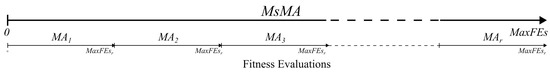
Figure 1. Uniform partitioning as defined by Equation (2).

This uniform distribution of computational resources raises the question of whether a single, longer run or multiple shorter runs is more effective. In most scenarios, the answer depends on stagnation. For instance, if stagnation occurs, it often makes sense to distribute computational resources across multiple restarts. However, a challenge arises in defining stagnation precisely—specifically, after how many evaluations ($MinSFEs$) can we consider stagnation to have occurred? Naturally, algorithms do not improve solutions with every evaluation, and the frequency of improvements typically decreases as the algorithm progresses. The optimal $MinSFEs$ value depends on the problem type and the exploration mechanisms of the MA.

In the proposed meta-optimization approach, which incorporates internal adaptive search partitioning based on a stagnation mechanism ($MsMA$), we maintain $MaxFEs$ as the primary stopping criterion, while $MinSFEs$ serves as an internal stopping/reset condition within the algorithm. The parameter $MinSFEs$ partitions each optimization run according to the algorithm’s stagnation criteria, where:

$$MaxFEs=\sum _{i=1}^{r}MaxFE{s}_i$$

(3)

Here, r represents the number of stagnation phases the algorithm has encountered excluding the current run. If the algorithm does not enter a stagnation phase, then $MaxFEs=MaxFE{s}_1$ with $r=1$.

In the worst-case scenario, such as when the first evaluation yields the best overall result, the maximum number of search partitions r is constrained by $MinSFEs$ and $MaxFEs$, as expressed in Equation (4):

$$r\le ⌈{\displaystyle \frac{MaxFEs}{MinSFEs}}⌉$$

(4)

The best solution found in each partition is stored, and the overall best solution $x_S^{\ast }$ is returned as the final result (Equation (5), Figure 2):

$$x_S^{\ast }=MsMA\left(M{A}_i(P,MinSFEs,MaxFE{s}_i)\right)|i=1,\dots ,r)$$

(5)

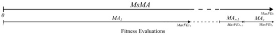
Figure 2. Partitioning based on stagnation as defined by Equation (5).

The key research question is whether this approach can enhance the performance of the selected MAs. In formal notation (Equations (6) and (7)), we aim to achieve:

$$\mathbb{E}\left[x_S^{\ast }\right]{\ge }_{\mathrm{opt}}\mathbb{E}\left[x^{\ast }\right]$$

(6)

where:

• $\mathbb{E}[·]$ denotes the expectation (average performance) over multiple optimization runs due to the stochastic nature of the algorithm.
• ${\ge }_{\mathrm{opt}}$ is a problem-dependent comparison operator, defined as:

  $$a{\ge }_{\mathrm{opt}}b=\left\{\begin{array}{cc}a\ge b,\hfill & \mathrm{if}\mathrm{the}\mathrm{objective}\mathrm{is}\mathrm{maximization},\hfill \\ a\le b,\hfill & \mathrm{if}\mathrm{the}\mathrm{objective}\mathrm{is}\mathrm{minimization}.\hfill \end{array}\right.$$

  (7)

MsMA Strategy: Implementation Details

To implement a meta-strategy for self-adaptive search partitioning at the meta-level, we propose using an algorithm wrapper that overrides execution. This strategy introduces an additional parameter, $MinSFEs$, used as an internal stopping criterion (Algorithm 1).

Algorithm 1. MsMA: A Meta-Level Strategy for Overcoming Stagnation

Require: A base metaheuristic $\mathtt{MA}$, $task$ with stopping criterion $MaxFEs$ and stagnation threshold $\mathtt{MinSFEs}$ Ensure: Best solution found   1: $\mathtt{bestSolution}\leftarrow \mathtt{null}$   2: $\mathtt{stagnationTask}\leftarrow \mathtt{newTaskStagnation}(\mathtt{task}.\mathtt{MaxFEs},\mathtt{task}.\mathtt{problem},\mathtt{MinSFEs})$   3: while $!\mathtt{stagnationTask}.\mathtt{isMaxFEsCriterionReached}\left(\right)$ do   4:     $\mathtt{tmp}\leftarrow \mathtt{MA}.\mathtt{execute}\left(\mathtt{stagnationTask}\right)$   5:     if $\mathtt{task}.\mathtt{problem}.\mathtt{isFirstBetter}(\mathtt{tmp},\mathtt{bestSolution})$ then   6:         $\mathtt{bestSolution}\leftarrow \mathtt{tmp}$   7:     end if   8:     $\mathtt{stagnationTask}.\mathtt{resetStagnationCounter}\left(\right)$   9:     $\mathtt{MA}.\mathtt{resetToDefaults}\left(\right)$ 10: end while 11: return $\mathtt{bestSolution}$

The idea behind this approach is that the algorithm consumes as many function evaluations as needed until stagnation is detected. Upon stagnation, a new search is initiated with a reduced evaluation budget. The number of evaluations already used is subtracted from $MaxFEs$, effectively decreasing the budget for subsequent runs. The optimization ceases once all evaluations are exhausted.

3.2. Synergizing MsMA and LTMA for Improved Performance

LTMA is a meta-level approach that enhances performance by leveraging memory to avoid re-evaluating previously generated solutions, commonly known as duplicates [11]. When an MA generates a new solution, it is stored in the memory. If the same solution is encountered again, the algorithm skips its evaluation and reuses the previously computed fitness value, leaving the fitness evaluation counter unchanged. Since memory lookup is significantly faster than fitness evaluation—especially in real-world optimization problems—this approach improves the computational performance substantially. LTMA is particularly beneficial when an algorithm repeatedly generates already-evaluated solutions, such as during stagnation phases, where duplicates are a common issue. Stagnation may not occur at a single point but can involve wandering within a region [36].

As a meta-level strategy, $MsMA$ can be combined with another meta-level approach, LTMA, to leverage synergistic effects. LTMA prevents redundant evaluations of previously encountered solutions, enhancing performance and accelerating convergence. The $LTMA$ approach can be applied in two ways: either to each MA partition run (Equation (8)) or to the entire $MsMA$ approach (Equation (9)).

$$\begin{array}{cc}\hfill resul{t}_s& =MsMA\left(LTMA\left(M{A}_i(P,MinSFEs,MaxFE{s}_i)\right)\right|i=1,\dots ,r\left)\right)\hfill \end{array}$$

(8)

$$\begin{array}{cc}\hfill resul{t}_s& =LTMA\left(MsMA\left(M{A}_i(P,MinSFEs,MaxFE{s}_i)\right)\right|i=1,\dots ,r\left)\right)\hfill \end{array}$$

(9)

Figure 3 illustrates the application of the LTMA strategy to MsMA, as detailed in Equations (8) and (9), showing MaxFEs partitioning for the top and bottom configurations.

Figure 3. Applying the LTMA strategy to MsMA, as defined by Equations (8) (top) and (9) (bottom).

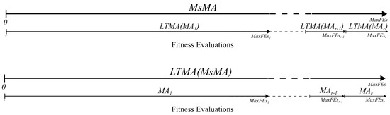
In the first approach (Equation (8)), LTMA is applied to each MA partition run, with a memory reset after each run, using the same or less memory compared to the second approach. In contrast, the second approach (Equation (9)) applies LTMA across all the partition runs $M{A}_i$, sharing information about previously explored areas between runs. This increases the likelihood of duplicate memory hits, as previously generated solutions remain in the LTMA memory.

The implementation of the $LTMA\left(MsMA\right)$ approach is presented in Algorithm 2. This algorithm resembles the $MsMA$ approach closely (Algorithm 1), with the addition of the $LTMA$ wrapper, which enhances performance by leveraging memory to avoid re-evaluating previously generated solutions.

Algorithm 2. LTMA(MsMA): Implementation Variant of MsMA Using LTMA

Require: A base metaheuristic $\mathtt{MA}$, $task$ with stopping criterion $MaxFEs$ and stagnation threshold $\mathtt{MinSFEs}$ Ensure: Best solution found   1: $\mathtt{bestSolution}\leftarrow \mathtt{null}$   2: $\mathtt{memStaTask}\leftarrow \mathbf{new}\mathbf{LTMA}\left(\mathbf{TaskStagnation}\right(\mathbf{task}.\mathbf{MaxFEs},\mathbf{task}.\mathbf{problem},\mathbf{MinSFEs}\left)\right)$   3: while $!\mathtt{memStaTask}.\mathtt{isMaxFEsCriterionReached}\left(\right)$ do   4:     $\mathtt{tmp}\leftarrow \mathtt{MA}.\mathtt{execute}\left(\mathtt{memStaTask}\right)$   5:     if $\mathtt{task}.\mathtt{problem}.\mathtt{isFirstBetter}(\mathtt{tmp},\mathtt{bestSolution})$ then   6:         $\mathtt{bestSolution}\leftarrow \mathtt{tmp}$   7:     end if   8:     $\mathtt{memStaTask}.\mathtt{resetStagnationCounter}\left(\right)$   9:     $\mathtt{MA}.\mathtt{resetToDefaults}\left(\right)$ 10: end while 11: return $\mathtt{bestSolution}$

As demonstrated in [11], modern computers have sufficient memory capacity for most optimization problems, storing only solutions and their fitness values. Therefore, we will evaluate the variant from Equation (9) in our experiments.

3.3. Time Complexity Analysis

Each meta-operator adds some overhead to the optimization process. The $MsMA$ strategy checks for stagnation and resets the algorithm’s internal state, which can be done in constant time. The time complexity of $MsMA$ is $O\left(1\right)$, as it performs only a few extra operations per function evaluation. Detecting stagnation adds minimal overhead, requiring a single if statement and a counter to check whether a new solution improves the current best.

The $LTMA$ strategy has a higher cost. Its time complexity is $O\left(n\right)$, where n is the number of function evaluations. Each evaluation involves checking for duplicates and updating memory, operations that take constant time on average. As shown in the original LTMA study [11], this overhead is small and generally negligible. There are edge cases, however. One occurs when algorithms, such as RS, rarely generate duplicate solutions. Another arises when fitness evaluations are extremely fast—comparable to a memory lookup in LTMA. In such cases, using LTMA can be slower than running the algorithm without it.

4. Experiments

The primary objective of this research is to promote meta-approaches by investigating the phenomenon of stagnation and exploring a meta-approach to overcome it. To achieve this, we selected several MAs for single-objective continuous optimization, specifically from evolutionary algorithms (EA) and swarm intelligence (SI). The parameters of the selected algorithms are kept at their default settings rather than being optimized. It is crucial to emphasize that the focus of this research is not to identify the best-performing MA but to analyze the effects of stagnation and evaluate the proposed method, which does not modify the core functioning of the optimization algorithm directly.

The selected SI algorithms are: Artificial Bee Colony (ABC) [59] with $limit={\displaystyle \frac{pop\_size·n}{2}}$ (where n denotes the problem dimensionality) and Particle Swarm Optimization (PSO) [23]. For EA, we selected: Self-Adapting Differential Evolution (jDE) [47], the less-known Manta Ray Foraging Optimization (MRFO) [60], and the Coral Reefs Optimization Algorithm (CRO) [61]. The source codes of all the algorithms used are included in the open-source EARS framework [62], specifically in the $algorithms.so$ package. We also included a simple random search (RS) as a baseline algorithm in all the experiments (Equation (10)).

$$MAs\in \{ABC,PSO,jDE,MRFO,CRO,RS\}$$

(10)

4.1. Statistical Analysis

Comparing stochastic algorithms requires complex statistical analysis involving multiple independent runs, average results, and Standard Deviations to determine significant differences. In practice, we aim for a simple representation of an algorithm’s performance, which can be achieved, for example, by assigning a rating to each algorithm. This approach is well-established and validated in fields such as chess ranking and video game matchmaking, where the goal is to pair opponents of similar strength [63,64,65,66]. Our experiments utilized the EARS framework with the default Chess Rating System for Evolutionary Algorithms (CRS4EA) [30,31]. CRS4EA integrates the Glicko-2 rating system, a widely used method in chess for ranking players. It assigns a rating to each algorithm based on its performance in benchmark tests, comparing the results against other algorithms in pairwise statistical evaluations—analogous to how chess players are ranked. CRS4EA operates by assessing algorithms based on their wins, draws, and losses in direct comparisons. These results determine each algorithm’s rating and confidence intervals. Every algorithm starts with a rating deviation (RD) of 350 and a rating of 1500, which is updated after each tournament. Over time, as the algorithm’s performance stabilizes, its RD is expected to decrease.

A study by [67] shows that the CRS4EA method performs on par with common statistical tests, like the Friedman test and the Nemenyi test. It also gives stable results, even with few independent runs. Another study by [68] finds CRS4EA comparable to the pDSC method. Together, these studies support CRS4EA as a reliable tool for comparing evolutionary algorithms.

To ensure reliable rating updates, it is recommended to set the minimum RD ($R{D}_{min}$) based on the number of matches and players in the tournament. In classical game scenarios, where players compete less frequently, an $R{D}_{min}$ of 50 is used typically. However, in our experiments, each MA competes against every other MA on 29 problems across 30 tournaments (requires, 30 independent runs for each problem), resulting in a high frequency of matches. Consequently, we set $R{D}_{min}$ to the minimum recommended value of 20. Reducing $R{D}_{min}$ below 20 is not advisable, as it may cause the ratings to converge too slowly [69,70]. We derived confidence intervals to compare algorithm performance using the computed ratings and RD values. The statistical significance of differences between algorithms is determined by the overlap (or lack thereof) of confidence intervals, calculated as $\pm 2RD$ around each algorithm’s rating. Non-overlapping confidence intervals indicate a statistically significant difference between algorithms with 95% confidence [69].

4.2. Benchmark Problems

Evaluating and comparing the performance of optimization algorithms requires a well-defined set of benchmark problems. Selecting a representative set that captures diverse optimization challenges ensures a fair and meaningful comparison. CEC benchmarks are used widely in the optimization community due to their extensive documentation and established credibility, making them suitable for our experiments. To prevent algorithms from exploiting specific problem characteristics, the benchmark problems are shifted and rotated, ensuring a more robust evaluation [71,72].

For our experiments, we utilized the latest CEC’24 benchmark suite [73], specifically the Single Bound Constrained Real-Parameter Numerical Optimization benchmark. This suite comprises 29 problems, including 2 unimodal, 7 multimodal, 10 hybrid, and 10 composition functions, designed to simulate various optimization challenges. The CEC’24 benchmark provides a comprehensive evaluation of optimization algorithms across a diverse range of problems.

4.3. MsMA: Meta-Level Strategy Experiment

For the evaluation of $MsMA$, we utilized the CEC’24 benchmark suite for the selected MAs, employing the CRS4EA rating system for ranking. In our experimental setup, we set the dimensionality of the problems to $n=30$, and defined the maximum number of function evaluations ($MaxFEs$) according to the benchmark specifications as $300,000$.

To evaluate the meta-approach, we addressed the experimental question: How does the introduction of the MsMA strategy influence the performance of MAs? This raises an additional question with the introduction of the new parameter $MinSFEs$: How does the MinSFEs parameter influence algorithm performance?

To investigate this, we tested $MinSFEs$ values at 2%, 4%, and 10% of $MaxFEs$, corresponding to 6000, $12,000$, and $30,000$ evaluations, respectively. We labeled each algorithm using the $MsMA$ strategy with suffixes _6, _12, and _30, reflecting the number of $MaxFEs$ evaluations in thousands. For example, when configured with $MinSFEs=6000$, the ABC algorithm is renamed ABC_6. Thus, an algorithm tested with different $MinSFEs$ values is treated as a distinct algorithm within the CRS4EA rating system. As a result, the ABC algorithm appears in the tournament four times—once with its default settings, and three times with different $MinSFEs$ values.

The experimental results are presented in a leaderboard table, displaying the ratings of MAs on the CEC’24 benchmark based on 30 tournament runs (requires, 30 independent runs for each problem). This setup is justified by previous findings showing that the CRS4EA rating system provides more reliable comparisons, and does not require a larger number of independent runs to achieve statistically robust results [67]. For each MA, we report its rank based on the overall rating, the rating deviation interval, the number of statistically significant positive (S+), and negative (S−) differences at the 95% confidence level (Table 1).

Table 1. The MsMA Leaderboard on the CEC’24 Benchmark.

Rank	MA	Rating	−2RD	+2RD	S+ (95% CI)	S− (95% CI)
1.	jDE_30	1974.69	1934.69	2014.69	+18
2.	jDE_6	1956.61	1916.61	1996.61	+18
3.	jDE_12	1916.00	1876.00	1956.00	+17
4.	jDE	1865.72	1825.72	1905.72	+17	−2
5.	PSO_30	1536.85	1496.85	1576.85	+13	−4
6.	PSO_6	1533.72	1493.72	1573.72	+13	−4
7.	PSO_12	1533.48	1493.48	1573.48	+13	−4
8.	PSO	1527.45	1487.45	1567.45	+13	−4
9.	MRFO_6	1437.60	1397.60	1477.60	+4	−8
10.	MRFO_12	1422.06	1382.06	1462.06	+3	−8
11.	ABC_30	1421.61	1381.61	1461.61	+3	−8
12.	ABC_12	1420.36	1380.36	1460.36	+3	−8
13.	ABC_6	1419.34	1379.34	1459.34	+3	−8
14.	ABC	1418.15	1378.15	1458.15	+3	−8
15.	MRFO_30	1397.95	1357.95	1437.95	+2	−8
16.	CRO_6	1395.20	1355.20	1435.20	+2	−8
17.	CRO_12	1368.82	1328.82	1408.82	+1	−8
18.	MRFO	1343.25	1303.25	1383.25	+1	−9
19.	CRO_30	1321.08	1281.08	1361.08	+1	−14
20.	CRO	1303.18	1263.18	1343.18	+1	−16
21.	RS	986.87	946.87	1026.87		−20

Note: The red font color highlights deviations discussed explicitly in the main text.

The $MsMA$ strategy proved highly successful, as all the algorithms incorporating $MsMA$ achieved higher ratings and ranks than their base variations (Table 1). However, not all the $MsMA$ variations resulted in statistically significant differences. For example, while jDE_6 and jDE_30 showed significant improvements over the core jDE, jDE_12 did not. For PSO, none of the $MsMA$ variations (PSO_6, PSO_12, PSO_30) exhibited a significant difference compared to the core PSO. In the case of MRFO, the variations were significantly different from the core MRFO, with MRFO_6 and MRFO_12 outperforming all the ABC variations. For ABC, no significant differences were observed among its variations, possibly due to its inherent limit parameter that restarts the search. For CRO, CRO_6 was significantly better than the core CRO (Table 1).

Regarding the $MinSFEs$ parameter, the results from Table 1 do not indicate a universally optimal value across all the algorithms. For instance, jDE, PSO, and ABC performed best with $MinSFEs$ set to 10% of $MaxFEs$, whereas MRFO and CRO achieved the best results with 2% of $MaxFEs$ (Table 1). The varying impact of the $MsMA$ strategy across the algorithms was expected, as each handles exploration and exploitation differently to avoid stagnation.

Further insights were gained by analyzing each algorithm’s wins, draws, and losses in pairwise comparisons. Since wins are more relevant for lower-performing algorithms, losses are crucial for top-performing ones, and draws provide less information, we focused on a detailed analysis of losses. Tables containing the results for wins and draws are provided in the Appendix A (Table A1 and Table A2).

Across 870 games, all the MAs lost at least some matches against every opponent (the first row in Table 2), except against the control RS algorithm (the last column in Table 2). A key observation is that the $MsMA$ strategy improved jDE’s performance against ABC (highlighted in blue); however, ABC_30 still found the best solution overall in 16 games. Additionally, most of jDE’s losses came from its improved variations; for example, jDE lost to jDE_30 a total of 760 times (Table 2). Interestingly, when comparing the jDE row with its top-performing variations (jDE_30, jDE_6, jDE_12), jDE often had fewer losses than its superior counterparts in most columns. In this case, partitioning the optimization process did not outperform full runs. This aligns with findings suggesting that extended search durations can help overcome stagnation and yield better solutions, indicating that longer runs may be advantageous when computational resources are less constrained [41].

Table 2. The Loss Outcomes for MS vs. MsMA on the CEC’24 Benchmark.

	jDE_30	jDE_6	jDE_12	jDE	PSO_30	PSO_6	PSO_12	PSO	MRFO_6	MRFO_12	ABC_30	ABC_12	ABC_6	ABC	MRFO_30	CRO_6	CRO_12	MRFO	CRO_30	CRO	RS
jDE_30	0	34	43	29	3	3	3	3	4	2	16	13	16	14	5	3	2	4	2	1	0
jDE_6	138	0	65	40	23	21	24	22	11	12	17	17	19	16	8	17	12	14	10	12	0
jDE_12	639	613	0	35	9	8	5	3	9	4	18	17	19	15	7	6	2	9	4	2	0
jDE	760	747	729	0	7	6	5	6	6	1	31	30	31	30	6	1	2	3	1	1	0
PSO_30	867	847	861	863	0	415	420	421	296	281	337	338	337	338	268	259	237	217	202	198	0
PSO_6	866	848	862	864	426	0	437	419	290	287	345	359	343	336	248	274	244	224	200	176	2
PSO_12	867	846	865	865	421	403	0	397	296	288	346	356	357	337	255	287	252	230	193	196	0
PSO	867	848	867	864	420	419	443	0	287	297	348	353	357	346	271	269	254	237	215	196	0
MRFO_6	863	857	859	864	550	554	549	559	0	410	389	393	384	376	372	393	368	314	326	281	1
MRFO_12	866	856	864	865	569	563	561	553	436	0	393	404	406	399	399	418	389	347	325	320	2
ABC_30	825	823	823	824	533	525	524	522	481	477	0	394	403	414	432	436	390	386	353	337	15
ABC_12	828	823	824	825	532	511	514	517	477	466	446	0	417	440	436	434	394	377	344	320	13
ABC_6	825	821	822	824	533	527	513	513	486	464	437	423	0	428	436	414	399	394	357	325	14
ABC	827	824	826	825	532	534	533	524	494	471	426	400	412	0	430	433	402	380	359	321	22
MRFO_30	863	859	860	862	583	602	597	581	477	454	438	434	434	440	0	430	410	357	342	321	1
CRO_6	867	853	864	869	611	596	583	601	477	452	434	436	456	437	440	0	413	358	348	359	2
CRO_12	868	858	868	868	633	626	618	616	502	481	480	476	471	468	460	457	0	395	392	354	7
MRFO	865	855	859	865	642	635	629	622	540	513	484	493	476	490	506	512	475	0	416	407	1
CRO_30	868	860	866	869	668	670	677	655	544	545	517	526	513	511	528	522	478	454	0	419	8
CRO	869	858	868	869	672	694	674	674	589	550	533	550	545	549	549	511	516	463	451	0	14
RS	870	870	870	870	870	868	870	870	869	868	855	857	856	848	869	868	863	869	862	856	0

Note: Red and blue font colors highlight deviations discussed explicitly in the main text.

To explore performance on individual problems, we investigated whether specific problems exist where the $MsMA$ strategy is particularly effective. Table 3 and Table 4 present the losses of each MA on problems F01 to F29.

Table 3. The Loss Outcomes of MAs on Individual Problems in the CEC’24 Benchmark (F01–F15).

	F01	F02	F03	F04	F05	F06	F07	F08	F09	F10	F11	F12	F13	F14	F15
jDE_30	0	0	113	33	6	2	2	2	2	2	2	2	2	2	2
jDE_6	0	0	130	248	0	5	5	5	5	5	5	5	5	5	5
jDE_12	0	0	149	69	6	50	50	50	50	50	50	50	50	50	50
jDE	0	0	124	39	104	89	89	89	89	89	89	89	89	89	89
PSO_30	306	333	344	194	363	305	222	196	352	192	228	241	230	212	282
PSO_6	324	454	369	227	435	353	237	196	337	188	226	209	204	174	244
PSO_12	327	421	370	190	393	347	203	172	328	194	242	208	213	238	309
PSO	316	275	389	215	393	326	239	197	340	192	242	219	216	214	302
MRFO_6	270	376	298	364	517	389	311	338	481	289	238	325	245	334	339
MRFO_12	296	289	331	332	520	403	305	380	465	308	212	323	251	326	325
ABC_30	234	525	136	468	0	305	481	518	223	520	443	464	454	435	313
ABC_12	237	535	161	418	0	307	491	533	231	512	464	498	449	464	298
ABC_6	241	523	132	463	0	313	485	504	226	509	438	522	440	496	268
ABC	219	561	167	475	0	300	467	497	237	540	435	433	470	428	287
MRFO_30	380	138	254	404	528	359	333	334	531	339	202	431	244	412	374
CRO_6	488	333	419	234	337	277	296	285	255	355	483	275	459	277	398
CRO_12	488	254	450	306	302	292	339	312	346	353	469	284	469	301	421
MRFO	459	136	284	400	532	447	370	367	475	330	213	435	221	440	432
CRO_30	476	216	488	307	268	394	356	331	339	342	494	304	484	357	471
CRO	459	209	509	314	272	403	385	360	354	357	491	349	502	412	457
RS	600	542	600	600	600	600	600	600	600	600	600	600	569	600	600

Note: Red and blue font colors highlight deviations discussed explicitly in the main text.

Table 4. The Loss Outcomes of MAs on Individual Problems in the CEC’24 Benchmark (F16–F29).

	F16	F17	F18	F19	F20	F21	F22	F23	F24	F25	F26	F27	F28	F29
jDE_30	2	2	2	2	2	2	2	2	2	2	2	2	2	2
jDE_6	5	5	5	5	5	5	5	5	5	5	5	5	5	5
jDE_12	50	50	50	50	50	50	50	50	50	50	50	50	50	50
jDE	89	89	89	89	89	89	89	89	89	89	89	89	89	89
PSO_30	279	202	269	369	331	126	300	300	313	290	329	360	324	210
PSO_6	292	210	194	342	303	120	286	301	328	313	288	378	297	221
PSO_12	269	223	226	324	299	120	309	311	328	293	308	330	343	219
PSO	310	204	238	355	325	120	273	320	340	314	364	353	336	231
MRFO_6	390	356	271	311	327	200	385	371	269	374	370	240	437	247
MRFO_12	383	374	296	314	394	256	435	341	230	385	425	303	416	317
ABC_30	278	380	500	287	261	468	242	340	253	211	210	262	225	481
ABC_12	270	414	480	286	237	463	216	261	268	207	211	260	245	522
ABC_6	283	388	529	263	278	453	283	196	271	195	199	279	239	539
ABC	289	399	481	271	278	462	302	325	242	230	190	234	241	515
MRFO_30	413	329	278	383	380	272	448	403	308	364	444	321	427	312
CRO_6	363	403	302	316	384	368	363	352	472	422	405	492	314	329
CRO_12	346	410	296	378	428	399	395	367	450	436	424	467	397	319
MRFO	429	324	394	362	420	345	494	463	443	500	496	302	443	329
CRO_30	460	466	401	462	426	402	387	423	515	497	413	433	398	388
CRO	466	440	365	504	449	419	402	446	490	481	444	480	438	341
RS	600	598	600	593	600	596	600	600	600	600	600	600	600	600

Note: The red font color highlights deviations discussed explicitly in the main text.

Problems F03 and F04 were the most challenging for the overall best-performing jDE and its variations (Figure A1 and Figure A2). The greatest improvement from $MsMA$ for jDE occurred on problem F05, where the losses decreased from 106 to 6 for jDE_12 and to 0 for jDE_6 and jDE_30 (Table 3).

Regarding ABC’s success against certain jDE runs (Table 2), Table 3 shows that ABC performed best on F05 with no losses (Figure A3), but it was the worst on F10, except for RS. Interestingly, the $MsMA$ strategy worsened MRFO’s performance slightly on problem F03 (highlighted in blue in Table 3). Compared to MRFO, CRO, and ABC, PSO had the fewest losses on problem F21 (Table 4). Tables with wins and draws for individual problems are provided in the Appendix A (Table A3 and Table A5).

4.4. LTMA(MsMA): Performance Experiment

To determine whether $LTMA\left(MsMA\right)$ complements and enhances performance, we conducted a similar experiment using the CEC’24 benchmark, following the same procedure as for $MsMA$ in Section 4.3. Here, $LTMA$ was applied to all $MsMA$ variations, and for comparison, we included the best-performing $MsMA$ variations of each MA from the previous experiment. Variations incorporating the $MsMA$ strategy are labeled with the suffix _LTMA, along with the corresponding $MsMA$ number label.

The experimental results are presented in a Leaderboard Table, displaying the ratings of MAs and their variations on the CEC’24 benchmark over 30 tournaments. For each MA, we report its rank based on overall rating, the rating deviation interval, the number of statistically significant positive (S+), and negative ($S-$) differences at the 95% confidence level (Table 5).

Table 5. The LTMA(MsMA) Leaderboard on the CEC’24 Benchmark.

Rank	MA	Rating	−2RD	+2RD	S+ (95% CI)	S− (95% CI)
1.	jDE_30	1951.69	1911.69	1991.69	+22
2.	jDE_LTMA_30	1945.87	1905.87	1985.87	+22
3.	jDE_LTMA_6	1929.01	1889.01	1969.01	+21
4.	jDE_LTMA_12	1917.70	1877.70	1957.70	+21
5.	jDE	1856.16	1816.16	1896.16	+21	−2
6.	PSO_LTMA_6	1557.01	1517.01	1597.01	+16	−5
7.	PSO_LTMA_12	1540.23	1500.23	1580.23	+16	−5
8.	PSO_LTMA_30	1518.02	1478.02	1558.02	+16	−5
9.	PSO_30	1516.40	1476.40	1556.40	+16	−5
10.	PSO	1510.43	1470.43	1550.43	+16	−5
11.	CRO_LTMA_12	1420.84	1380.84	1460.84	+3	−10
12.	MRFO_LTMA_6	1420.29	1380.29	1460.29	+3	−10
13.	CRO_LTMA_6	1415.25	1375.25	1455.25	+3	−10
14.	MRFO_6	1412.70	1372.70	1452.70	+3	10
15.	ABC_LTMA_12	1396.66	1356.66	1436.66	+2	−10
16.	ABC_LTMA_30	1396.37	1356.37	1436.37	+2	−10
17.	MRFO_LTMA_30	1394.67	1354.67	1434.67	+2	−10
18.	ABC_30	1394.08	1354.08	1434.08	+2	−10
19.	ABC	1393.84	1353.84	1433.84	+2	−10
20.	MRFO_LTMA_12	1393.41	1353.41	1433.41	+2	−10
21.	ABC_LTMA_6	1380.61	1340.61	1420.61	+2	−10
22.	CRO_LTMA_30	1375.58	1335.58	1415.58	+2	−10
23.	CRO_6	1370.09	1330.09	1410.09	+2	−10
24.	MRFO	1324.75	1284.75	1364.75	+1	−14
25.	CRO	1282.19	1242.19	1322.19	+1	−23
26.	RS	986.17	946.17	1026.17		−25

Note: Red and blue font colors highlight deviations discussed explicitly in the main text.

Applying the LTMA strategy to all MsMA variants yielded performance improvements across most MA variants, except for jDE_30, the top performer from the prior experiment (Table 1 and Table 5). The minor rating difference between jDE_30 and jDE_LTMA_30 is statistically insignificant, and may stem from the stochastic nature of the MAs. Alternatively, LTMA may be less effective when an MA reaches the global optima consistently, as additional evaluations from duplicates fail to enhance solutions. Another possibility is the link between duplicate evaluations and stagnation, where mitigating one issue partially alleviates the other.

For PSO, there was no significant difference between PSO and its $LTMA$-enhanced variations (PSO_LTMA_6, PSO_LTMA_12, PSO_LTMA_30). The most substantial improvement was observed in CRO with $LTMA\left(MsMA\right)$, where the rating increased from 1370.09 to 1420.87, surpassing all MRFO and ABC variations (Table 5). As expected, self-adaptive MAs like jDE and ABC showed limited gains with $LTMA\left(MsMA\right)$, as they rarely enter stagnation cycles. The experiment also revealed a possible negative impact of $LTMA\left(MsMA\right)$ on ABC, where ABC_LTMA_6 performed worse than the base ABC (Table 5), similar to ABC_6’s near-identical rating to the core ABC in the previous experiment (Table 1). This may be due to $LTMA$’s precision, set to nine decimal places in the search space, where small changes could lead to larger fitness variations, resulting in more draws and fewer wins (draws were determined with a threshold of $1\times {10}^{-6}$).

Further understanding was gained by analyzing the losses in MA vs. MA comparisons, which provide detailed insights into relative performance. The results are presented in Table 6.

Table 6. The LTMA(MsMA) Loss Outcomes for MS vs. MsMA for the CEC’24 Benchmark.

	jDE_30	jDE_LTMA_30	jDE_LTMA_6	jDE_LTMA_12	jDE	PSO_LTMA_6	PSO_LTMA_12	PSO_LTMA_30	PSO_30	PSO	CRO_LTMA_12	MRFO_LTMA_6	CRO_LTMA_6	MRFO_6	ABC_LTMA_12	ABC_LTMA_30	MRFO_LTMA_30	ABC_30	ABC	MRFO_LTMA_12	ABC_LTMA_6	CRO_LTMA_30	CRO_6	MRFO	CRO	RS
jDE_30	0	404	36	39	29	3	3	5	3	3	4	5	3	4	16	13	4	16	14	5	14	2	3	4	1	0
jDE_LTMA_30	349	0	348	354	36	7	4	9	7	7	7	7	8	5	19	16	5	19	18	5	16	5	6	5	3	0
jDE_LTMA_6	55	434	0	74	51	32	30	29	29	28	30	27	30	22	24	22	22	26	17	22	25	29	29	19	21	0
jDE_LTMA_12	402	422	372	0	39	19	17	17	19	16	19	13	20	9	18	15	8	18	17	8	17	12	13	10	10	0
jDE	760	750	746	747	0	5	1	6	7	6	4	5	3	6	30	30	3	31	30	5	30	1	1	3	1	0
PSO_LTMA_6	867	863	838	851	865	0	397	378	386	355	270	246	263	248	287	294	227	295	296	243	289	235	220	206	149	1
PSO_LTMA_12	867	866	840	853	868	442	0	403	394	368	295	280	265	260	320	308	259	311	315	249	305	250	234	206	160	1
PSO_LTMA_30	865	860	841	853	864	462	437	0	430	418	296	286	292	291	341	342	290	331	332	273	326	275	259	228	191	0
PSO_30	867	863	841	851	863	455	447	410	0	421	303	293	296	296	352	330	288	337	338	292	325	280	259	217	198	0
PSO	867	863	842	854	864	485	472	420	420	0	298	283	319	287	351	350	294	348	346	269	330	280	269	237	196	0
CRO_LTMA_12	866	863	840	851	866	600	575	574	567	572	0	447	369	410	402	386	382	379	382	404	394	397	389	332	286	0
MRFO_LTMA_6	864	862	841	855	864	598	563	558	551	560	423	0	432	415	364	369	397	381	356	411	367	399	377	317	300	0
CRO_LTMA_6	867	862	840	850	867	607	605	578	574	551	501	438	0	425	374	368	391	361	365	405	370	416	407	336	290	2
MRFO_6	863	863	846	858	864	598	585	554	550	559	460	422	445	0	393	384	393	389	376	407	390	399	393	314	281	1
ABC_LTMA_12	825	822	816	822	825	583	550	529	518	519	468	506	496	477	0	432	476	422	441	456	386	409	416	392	310	17
ABC_LTMA_30	828	825	818	825	825	576	562	528	540	520	484	501	502	486	408	0	463	410	413	458	373	413	435	383	326	17
MRFO_LTMA_30	863	863	846	859	862	624	592	560	563	557	488	447	479	452	394	407	0	394	401	434	388	422	414	355	320	2
ABC_30	825	822	814	822	824	575	559	539	533	522	491	489	509	481	418	430	476	0	414	457	380	413	436	386	337	15
ABC	827	823	823	823	825	574	555	538	532	524	488	514	505	494	399	427	469	426	0	457	375	418	433	380	321	22
MRFO_LTMA_12	861	860	844	859	862	603	597	574	556	578	466	433	465	436	414	412	419	413	413	0	410	430	416	353	325	0
ABC_LTMA_6	827	825	815	823	825	581	565	544	545	540	476	503	500	480	454	467	482	460	465	460	0	421	436	402	342	11
CRO_LTMA_30	868	865	841	858	869	635	620	595	590	590	473	471	454	471	461	457	448	457	452	440	449	0	418	369	323	7
CRO_6	867	864	841	857	869	650	636	611	611	601	481	493	463	477	454	435	456	434	437	454	434	452	0	358	359	2
MRFO	865	861	850	859	865	653	653	630	642	622	538	536	534	540	478	487	504	484	490	505	468	501	512	0	407	1
CRO	869	867	849	860	869	721	710	679	672	674	584	570	580	589	560	544	550	533	549	545	528	547	511	463	0	14
RS	870	870	870	870	870	869	869	870	870	870	870	870	868	869	853	853	868	855	848	870	859	863	868	869	856	0

Note: Red and blue font colors highlight deviations discussed explicitly in the main text.

The data from Table 6 reveal that jDE_LTMA_30 lost to jDE_30; however, jDE_LTMA_30 had fewer losses against jDE_30 (349) than jDE_30 had against jDE_LTMA_30 (404, highlighted in red in Table 6). The most significant rating differences for jDE_LTMA_30 stemmed from losses against jDE_LTMA_6 and jDE_LTMA_12 (highlighted in blue in Table 6). This suggests that $LTMA$ utilized better solutions on average but with less precision, leading to more losses against higher-precision solutions. For deeper analysis, the results for wins and draws are provided in the Appendix A (Table A7 and Table A8).

To gain additional insights into performance on individual problems, we present the losses of each MA for specific problems in Table 7 and Table 8.

Table 7. The Loss Outcomes of MAs with LTMA on Individual Problems in the CEC’24 Benchmark (F01–F15).

	F01	F02	F03	F04	F05	F06	F07	F08	F09	F10	F11	F12	F13	F14	F15
jDE_30	0	0	147	46	8	18	18	18	18	18	18	18	18	18	18
jDE_LTMA_30	0	0	170	102	9	41	41	41	41	41	41	41	41	41	41
jDE_LTMA_6	0	36	159	524	0	17	17	17	17	17	17	17	17	17	17
jDE_LTMA_12	0	0	178	248	0	46	46	46	46	46	46	46	46	46	46
jDE	0	0	154	43	134	120	120	120	120	120	120	120	120	120	120
PSO_LTMA_6	373	556	472	216	534	458	277	274	441	241	342	221	271	224	265
PSO_LTMA_12	369	525	448	276	472	438	317	223	447	236	317	276	284	242	308
PSO_LTMA_30	413	408	435	258	449	452	346	241	436	246	276	292	274	284	364
PSO_30	383	347	444	267	422	420	317	249	468	233	281	310	300	275	411
PSO	395	265	477	288	457	449	318	246	452	233	299	298	278	286	422
CRO_LTMA_12	690	460	565	212	450	273	318	367	308	439	561	304	513	363	402
MRFO_LTMA_6	392	410	371	409	670	437	438	466	636	376	284	451	316	400	397
CRO_LTMA_6	720	550	624	191	522	335	256	339	238	486	547	408	458	404	319
MRFO_6	351	411	380	478	652	514	405	447	613	360	294	442	323	440	455
ABC_LTMA_12	327	663	189	575	0	416	633	671	333	633	559	647	555	592	426
ABC_LTMA_30	286	686	223	568	0	418	606	644	289	639	578	599	606	561	401
MRFO_LTMA_30	407	168	392	490	641	496	430	519	653	452	261	435	304	526	526
ABC_30	307	652	159	597	0	423	630	646	321	657	583	605	586	578	437
ABC	297	693	191	615	0	405	611	622	318	672	567	566	601	566	404
MRFO_LTMA_12	427	295	346	470	657	476	433	455	602	413	247	453	309	433	445
ABC_LTMA_6	316	652	185	583	0	429	614	657	331	639	593	651	578	640	452
CRO_LTMA_30	566	312	604	306	360	359	350	320	369	438	611	357	641	404	557
CRO_6	592	343	544	312	387	373	408	373	349	438	611	372	598	376	550
MRFO	545	163	356	509	665	591	485	480	619	421	266	563	279	564	565
CRO	544	216	650	416	312	538	507	461	477	448	623	450	655	542	594
RS	750	675	750	750	750	750	750	750	750	750	750	750	721	750	750

Note: The red font color highlights deviations discussed explicitly in the main text.

Table 8. The Loss Outcomes of MAs with LTMA on Individual Problems in the CEC’24 Benchmark (F16–F29).

	F16	F17	F18	F19	F20	F21	F22	F23	F24	F25	F26	F27	F28	F29
jDE_30	18	18	18	18	18	18	18	18	18	18	18	18	18	18
jDE_LTMA_30	41	41	41	41	41	41	41	41	41	41	41	41	41	41
jDE_LTMA_6	17	17	17	17	17	17	17	17	17	17	17	17	17	17
jDE_LTMA_12	46	46	46	46	46	46	46	46	46	46	46	46	46	46
jDE	120	120	120	120	120	120	120	120	120	120	120	120	120	120
PSO_LTMA_6	285	280	195	332	385	150	382	374	320	303	321	428	398	251
PSO_LTMA_12	339	292	251	363	386	150	387	398	431	344	360	400	409	231
PSO_LTMA_30	431	261	266	427	399	150	454	420	411	421	401	457	413	298
PSO_30	361	258	355	498	444	160	415	420	396	405	438	435	437	273
PSO	417	267	303	491	431	150	375	447	428	430	480	429	446	287
CRO_LTMA_12	382	451	383	422	430	497	379	394	587	511	483	613	389	387
MRFO_LTMA_6	456	414	424	420	471	208	499	469	382	443	499	362	535	389
CRO_LTMA_6	345	443	380	323	388	578	325	375	673	491	392	668	374	498
MRFO_6	517	468	360	431	441	254	526	516	334	489	490	297	568	331
ABC_LTMA_12	372	513	654	408	354	595	297	278	361	275	304	290	329	664
ABC_LTMA_30	389	537	601	378	465	616	385	333	329	256	258	313	304	651
MRFO_LTMA_30	534	407	400	434	481	331	532	521	289	471	560	346	562	418
ABC_30	385	499	639	402	331	610	344	428	325	287	288	315	322	611
ABC	399	541	613	384	353	601	412	416	305	320	236	289	328	647
MRFO_LTMA_12	571	445	420	507	472	262	562	529	397	521	577	380	512	383
ABC_LTMA_6	365	521	674	385	317	582	310	235	395	293	350	509	319	674
CRO_LTMA_30	487	584	375	537	498	451	441	471	579	568	498	549	464	425
CRO_6	490	523	412	426	511	445	507	488	598	566	537	612	432	423
MRFO	561	422	513	479	543	443	636	602	554	651	646	360	584	420
CRO	614	575	482	657	600	528	532	586	606	638	582	590	575	439
RS	750	749	750	746	750	746	750	750	750	750	750	750	750	750

Note: The red font color highlights deviations discussed explicitly in the main text.

The results from Table 7 show that jDE_LTMA_6 would be the clear winner if problem F04 were excluded, where it performed poorly with 524 losses. Notably, RS achieved 75 wins on F02, corresponding to 675 losses (Table 7 and Table A9), and ABC and its variations remained unbeaten on F05 (Figure A3).

Analysis of the top five MAs showed consistent performance across problems F16 to F29 (Table 8). In contrast, the bottom-performing MAs like ABC, MRFO_LTMA_6, and ABC_LTMA_6 exhibited relatively large deviations despite fewer losses relative to their overall rank (Table 8). Additional Tables for wins and draws on individual problems are provided in the Appendix A (Table A9, Table A10, Table A11 and Table A12).

For a comparison involving more recent MAs, see Appendix A.4.

4.5. Experiment: Real-World Optimization Problem

The selected real-world problem addresses the optimization of load flow analysis (LFA) in unbalanced power distribution networks with incomplete data. The example showed on Figure 4 illustrates a typical residential power distribution network with multiple consumers, each connected to three-phase supply lines. The network is characterized by its unbalanced nature, where the power consumption of each consumer may vary across the three phases. Where blue nodes represent consumers with partial measurements, green nodes represent consumers without measurements, and red is the transformer with complete measurement [74].

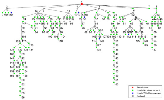
Figure 4. Power Distribution Network Topology.

Due to limitations in the measurement infrastructure, comprehensive per-phase power consumption data for all consumers is often unavailable, resulting in sparse datasets. The optimization problem focuses on estimating the unmeasured per-phase active and reactive power consumption for consumers, given partial measurements of per-phase voltages and power.

The objective of the proposed optimization algorithm is to minimize the discrepancy between the calculated and measured per-phase voltages at a subset of monitored nodes (n). Specifically, the algorithm estimates: (1) per-phase active ($P_1,P_2,P_3$) and reactive power ($Q_1,Q_2,Q_3$) for unmeasured consumers ($n\in [1\dots m]$), and (2) the distribution of measured ($n\in [m+1\dots j]$) three-phase active power across individual phases for consumers with partial measurements ($Pmax$). The optimization does not constrain the solution to match measured aggregate power values at the network’s supply point, allowing for the estimation of network losses. The LFA approach used in the paper was Backward Forward Sweep (BFS) [75].

Network losses, which may account for up to 5% of power in larger systems, are assumed negligible in this problem to simplify the optimization model by excluding the loss parameters. The optimization was subject to the following constraints:

1.

Maximum three-phase active power consumption per consumer ($Pmax$), reflecting realistic load limits (Equation (11)).

$$Pnerr=\sum _{n=1}^j\sum _{i=1}^{3}max(P_{n,i}-Pma{x}_n,0)$$

(11)

2.

Maximum per-phase current, constrained by fuse ($Ifuse$) ratings to ensure safe operation (Equation (12)).

$$Ierr=\sum _{n=1}^j\sum _{i=1}^{3}max(I_{n,j}-Ifus{e}_n,0)$$

(12)

3.

Sum of three-phase active (P) and reactive power (Q) for consumptions, reflecting transformer measured values ($P_{sum}$,$Q_{sum}$) (Equations (13), and (14)).

$$Perr=\sum _{i=1}^{3}abs(P_{sum,i}-\sum _{n=1}^j{P}_{n,i})$$

(13)

$$Qerr=\sum _{i=1}^{3}abs(Q_{sum,i}-\sum _{n=1}^j{Q}_{n,i})$$

(14)

4.

Inductive-only reactive power consumption, preventing unintended reactive power exchange between consumers.

The optimization goal is to minimize the difference ($Udif$) between the calculated ($Ucalc$) and measured ($Umeas$) per-phase voltages at monitored nodes, skipping the first node-transformer (Equation (15)). The BFS algorithm computes the voltage at each node based on the estimated power consumption.

$$Udif=\sum _{\begin{array}{c}n=2\end{array}}^j\sum _{i=1}^{3}abs(Umea{s}_{n,i}-Ucal{c}_{n,i})$$

(15)

Based on the optimization goal and constraints, the fitness function is defined by Equation (16).

$$F_{fitness}=Udif+Pnerr+Qerr+Perr+Ierr$$

(16)

These constraints ensure that the estimated power consumption remains physically plausible and adheres to the operational limits of the distribution network. The problem is formulated to handle the stochastic and nonlinear nature of load flow analysis, leveraging sparse data to achieve accurate voltage estimation.

The experimental setup and statistical analysis follow the configuration detailed in Section 4.1. For the LFA problem, the maximum number of function evaluations was set to $MaxFEs=100,000$. To show the concept and limit the number of parameters we have limited ourselves to the “leftmost” feeder with five nodes beside the transformer (Figure 4): one transformer node where all the data are known, one measured node with known per-phase voltages U and total P, and three unmeasured nodes. For the unmeasured nodes, the optimization estimates per-phase P and Q. Additionally, for the measured node, the total three-phase active power is distributed across the three phases.

In total, the optimization involves 24 parameters: 9 parameters for the unmeasured nodes (3 nodes × 3 phases for P), 12 parameters for reactive power (4 nodes × 3 phases for Q), and 3 parameters for the per-phase distribution of active power at the measured node.

The performance of various metaheuristic algorithms on the LFA problem is summarized in Table 9.

Table 9. The MAs Leaderboard on The LFA Problem.

Rank	MA	Rating	−2RD	+2RD	S+ (95% CI)	S− (95% CI)
1.	MRFO_LTMA_12	1843.00	1803.00	1883.00	+32
2.	jDE_LTMA_12	1770.45	1730.45	1810.45	+23
3.	MRFO_LTMA_30	1764.53	1724.53	1804.53	+22
4.	jDE_LTMA_30	1763.05	1723.05	1803.05	+22
5.	MRFO_6	1761.57	1721.57	1801.57	+21	−1
6.	jDE_LTMA_6	1756.14	1716.14	1796.14	+21	−1
7.	CRO_LTMA_30	1751.70	1711.70	1791.70	+20	−1
8.	jDE_12	1741.83	1701.83	1781.83	+18	−1
9.	jDE	1735.41	1695.41	1775.41	+17	−1
10.	MRFO_LTMA_6	1725.54	1685.54	1765.54	+16	−1
11.	jDE_30	1717.64	1677.64	1757.64	+16	−1
12.	jDE_6	1709.25	1669.25	1749.25	+16	−1
13.	CRO_6	1698.40	1658.40	1738.40	+15	−1
14.	CRO_LTMA_12	1686.06	1646.06	1726.06	+15	−2
15.	MRFO_12	1682.60	1642.60	1722.60	+15	−4
16.	CRO_30	1672.73	1632.73	1712.73	+15	−6
17.	CRO_12	1666.81	1626.81	1706.81	+15	−7
18.	MRFO	1662.37	1622.37	1702.37	+15	−7
19.	MRFO_30	1659.90	1619.90	1699.90	+15	−8
20.	CRO_LTMA_6	1652.99	1612.99	1692.99	+15	−9
21.	CRO	1627.82	1587.82	1667.82	+15	−12
22.	ABC_LTMA_12	1320.36	1280.36	1360.36	+8	−21
23.	ABC_30	1308.51	1268.51	1348.51	+8	−21
24.	ABC	1301.60	1261.60	1341.60	+8	−21
25.	ABC_LTMA_30	1292.72	1252.72	1332.72	+8	−21
26.	ABC_12	1290.75	1250.75	1330.75	+8	−21
27.	ABC_6	1273.97	1233.97	1313.97	+8	−21
28.	ABC_LTMA_6	1256.20	1216.20	1296.20	+7	−21
29.	PSO_LTMA_6	1187.11	1147.11	1227.11	+3	−27
30.	PSO_LTMA_12	1168.35	1128.35	1208.35	+2	−28
31.	PSO_6	1152.56	1112.56	1192.56	+1	−28
32.	PSO_LTMA_30	1128.87	1088.87	1168.87	+1	−28
33.	PSO_12	1119.99	1079.99	1159.99	+1	−28
34.	PSO_30	1092.85	1052.85	1132.85	+1	−29
35.	PSO	1074.59	1034.59	1114.59	+1	−30
36.	RS	981.80	941.80	1021.80		−35

Note: The red font color highlights deviations discussed explicitly in the main text.

The results demonstrate that the MRFO algorithm, enhanced with LTMA and MsMA strategies, outperformed the other algorithms significantly, achieving the highest rating value of 1843, which is significantly better than the 32 other algorithms variations. The jDE algorithm, also enhanced with LTMA and MsMA strategies, ranks second with a rating value of 1770.45, outperforming the 23 other algorithms significantly. Furthermore, all the tested LTMA configurations combined with MsMA surpassed the performance of their respective baseline algorithms (marked with the red color in Table 5). Notably, MRFO and CRO, despite being among the lowest-performing algorithms on the CEC’24 benchmark (Table 5), achieved top or near-top performances with these strategies.

For a comparison involving more recent MAs, see Appendix A.4.

5. Discussion

The stagnation problem is as old as MAs themselves. It is well recognized that stagnation occurs in MAs frequently, often when the algorithm struggles to transition from the exploitation phase back to effective exploration. Researchers have tackled this issue through various strategies, among which self-adaptive algorithms have demonstrated notable success. Self-adaptation can be applied to different aspects of MAs, ranging from adjusting the internal parameters dynamically (e.g., mutation rates or learning factors), to introducing individual-level control, or modifying the population size based on stagnation detection [48,76]. Another common practice is to use stagnation as a stopping criterion. This approach serves a dual purpose: it prevents the waste of computational resources when progress stalls, while also avoiding premature termination when other criteria (e.g., $MaxFEs$ or iteration limits) might otherwise halt optimization too early [29].

In this study, we proposed a meta-level strategy, $MsMA$, that partitions the search process based on stagnation detection. A key advantage of meta-level strategies like $MsMA$ is their generality: they can be applied across different core MAs without requiring modifications to the underlying algorithm. This facilitates fairer comparisons and reusable optimization logic across MA variants, eliminating the need to define and publish a new variant for every core MA. For instance, one might claim to have developed five novel MAs when, in reality, only a self-adaptive stagnation mechanism has been applied to the existing core MAs. Such an approach offers little benefit to the community, as it obscures the new MA’s behavior and its performance relative to the established methods. Additionally, because meta-strategies operate by wrapping core algorithms, they can be nested or chained with other meta-level mechanisms. This was demonstrated through the integration of $LTMA$ with $MsMA$, illustrating how different meta-strategies can synergize to enhance performance and convergence.

However, not all strategies are suitable for meta-level abstraction. Generally, strategies with broader generalization capabilities are better suited for meta-level applications. A balance must be struck between what can be externalized at the meta-level and what must remain embedded within the core algorithm. For example, global parameters such as $MaxFEs$ (utilized by $MsMA$) and solution evaluation control (leveraged by $LTMA$) are well suited for meta-level adaptation. In contrast, tightly coupled internal components—such as parent selection or recombination operators for generating new solution candidates—are challenging to expose or modify externally due to their interdependencies at each optimization step.

During the experimentation and development, we encountered several practical challenges. Notably, the proposed method employs a reset mechanism based on a stopping condition termed $MinSFEs$, which partitions $MaxFEs$ into unequal partitions depending on the algorithm’s performance. Consequently, the final partition,$MaxFE{s}_{last}$, can sometimes be extremely small—occasionally even smaller than the population size. This can cause errors in algorithms that require a minimum number of evaluations to function correctly. To address this, we propose that the algorithms implement a $\mathtt{getMinimalEvaluation}$ method, which returns the minimum number of evaluations needed for safe operation. If the remaining evaluation budget falls below this threshold, the algorithm can skip execution, avoiding runtime errors. To utilize otherwise unused evaluations effectively, we applied a fallback random search strategy, ensuring that even small remaining budgets contribute to the optimization process.

6. Conclusions

This study tackled the persistent challenge of stagnation in MAs by introducing a general meta-level strategy, $MsMA$, designed to enhance optimization performance. The proposed strategy improved performance across all tested MAs on the 29 CEC’24 benchmark problems, boosting the rankings of jDE, MRFO, and CRO significantly. Notably, applying $MsMA$ altered the relative rankings of some algorithms; for instance, MRFO surpassed ABC in overall performance (Table 1).

Beyond its general applicability, the study demonstrated the feasibility of nesting meta-strategies through the integration of $LTMA$ with $MsMA$, highlighting their synergistic potential. Leveraging $LTMA$ enhanced the performance of most $MsMA$ variations further, with CRO showing the greatest improvement—specifically, CRO_LTMA_12 overtook MRFO_LTMA_6 in the rankings (Table 5).

For the LFA optimization problem, the experimental results demonstrate that nearly all algorithms enhanced with MsMA and LTMA strategies outperformed their baseline counterparts significantly, with the exception of the ABC algorithm. Notably, the MRFO algorithm, despite being among the lowest-performing algorithms on the CEC’24 benchmark (Table 5), achieved the highest performance on the LFA problem, with a rating value of 1843 (Table 9). This suggests that MRFO’s search mechanisms or parameter configurations are particularly well-suited to the characteristics of the LFA problem, highlighting its potential for real-world power distribution optimization.

Future work should focus on developing more advanced meta-strategies tailored to the specific characteristics of both the core algorithm and the problem domain. Additionally, the $MsMA$ framework could be extended to other optimization contexts, such as multi-objective, dynamic, and constrained optimization.

This study encourages further research into meta-level strategies and their integration, opening new avenues for a better understanding of the general strategies and characteristics of modern MAs.

Appendix A.1. Selected CEC’24 Benchmark Problems

This subsection presents the CEC’24 benchmark problems selected for the experiments. The accompanying Figures depict these benchmark functions in their original form, without applying rotation (rotation matrix M) or shifting (shift vector o). For enhanced visualization, the functions are illustrated in two dimensions, although they are defined in n dimensions, where n represents the problem’s dimensionality. For further details on the CEC’24 benchmark suite, refer to the competition documentation [71,72].

$$F03\left(\mathbf{x}\right)=\sum _{i=1}^{n-1}\left[100{(z_{i+1}-z_i^2)}^2+{(z_i-1)}^2\right],\mathrm{where}\mathbf{z}=\mathbf{M}(\mathbf{x}-\mathbf{o}),\mathrm{subject}\mathrm{to}\mathbf{x}\in {[-100,100]}^n$$

(A1)

$$F04\left(\mathbf{x}\right)=10D+\sum _{i=1}^D\left[z_i^2-10cos\left(2\pi z_i\right)\right],\mathrm{where}\mathbf{z}=\mathbf{M}(\mathbf{x}-\mathbf{o}),\mathrm{subject}\mathrm{to}\mathbf{x}\in {[-100,100]}^D$$

(A2)

$$F05\left(\mathbf{x}\right)=\sum _{i=1}^{n-1}\left[0.5+{\displaystyle \frac{{sin}^2\left(\sqrt{z_i^2+z_{i+1}^2}\right)-0.5}{{\left(1+0.001(z_i^2+z_{i+1}^2)\right)}^2}}\right],\mathrm{where}\mathbf{z}=\mathbf{M}(\mathbf{x}-\mathbf{o}),\mathrm{subject}\mathrm{to}\mathbf{x}\in {[-100,100]}^n$$

(A3)

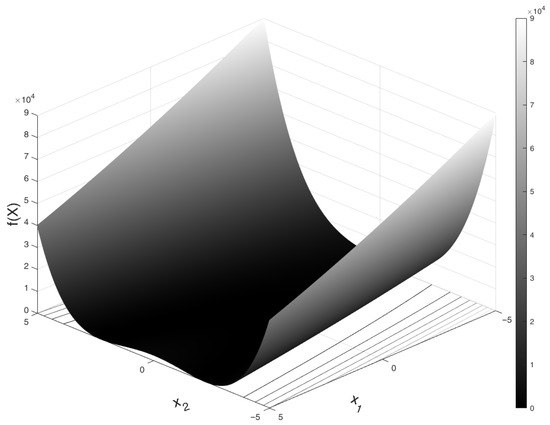
Figure A1. F03: Rosenbrock’s Function.

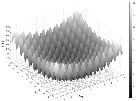
Figure A2. F04: Rastrigin’s Function (not rotated or shifted).

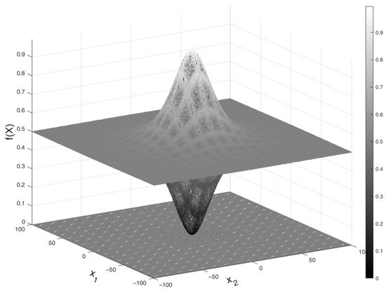
Figure A3. F05: Schaffer’s Function.

Appendix A.2. The MsMA Experiment

The following Tables present the results of the $MsMA$ experiment on the CEC’24 benchmark. They report the number of wins and draws for each algorithm, based on pairwise comparisons and their performance on individual benchmark problems from F01 to F29. Additional Tables showing the number of losses are provided in Appendix A.

Table A1. MsMA Draw Outcomes in MA vs. MA Comparisons on the CEC’24 Benchmark.

	jDE_30	jDE_6	jDE_12	jDE	PSO_30	PSO_6	PSO_12	PSO	MRFO_6	MRFO_12	ABC_30	ABC_12	ABC_6	ABC	MRFO_30	CRO_6	CRO_12	MRFO	CRO_30	CRO	RS
jDE_30	0	698	188	81	0	1	0	0	3	2	29	29	29	29	2	0	0	1	0	0	0
jDE_6	698	0	192	83	0	1	0	0	2	2	30	30	30	30	3	0	0	1	0	0	0
jDE_12	188	192	0	106	0	0	0	0	2	2	29	29	29	29	3	0	0	2	0	0	0
jDE	81	83	106	0	0	0	0	0	0	4	15	15	15	15	2	0	0	2	0	0	0
PSO_30	0	0	0	0	0	29	29	29	24	20	0	0	0	0	19	0	0	11	0	0	0
PSO_6	1	1	0	0	29	0	30	32	26	20	0	0	0	0	20	0	0	11	0	0	0
PSO_12	0	0	0	0	29	30	0	30	25	21	0	0	0	0	18	0	0	11	0	0	0
PSO	0	0	0	0	29	32	30	0	24	20	0	0	0	0	18	0	0	11	0	0	0
MRFO_6	3	2	2	0	24	26	25	24	0	24	0	0	0	0	21	0	0	16	0	0	0
MRFO_12	2	2	2	4	20	20	21	20	24	0	0	0	0	0	17	0	0	10	0	0	0
ABC_30	29	30	29	15	0	0	0	0	0	0	0	30	30	30	0	0	0	0	0	0	0
ABC_12	29	30	29	15	0	0	0	0	0	0	30	0	30	30	0	0	0	0	0	0	0
ABC_6	29	30	29	15	0	0	0	0	0	0	30	30	0	30	0	0	0	0	0	0	0
ABC	29	30	29	15	0	0	0	0	0	0	30	30	30	0	0	0	0	0	0	0	0
MRFO_30	2	3	3	2	19	20	18	18	21	17	0	0	0	0	0	0	0	7	0	0	0
CRO_6	0	0	0	0	0	0	0	0	0	0	0	0	0	0	0	0	0	0	0	0	0
CRO_12	0	0	0	0	0	0	0	0	0	0	0	0	0	0	0	0	0	0	0	0	0
MRFO	1	1	2	2	11	11	11	11	16	10	0	0	0	0	7	0	0	0	0	0	0
CRO_30	0	0	0	0	0	0	0	0	0	0	0	0	0	0	0	0	0	0	0	0	0
CRO	0	0	0	0	0	0	0	0	0	0	0	0	0	0	0	0	0	0	0	0	0
RS	0	0	0	0	0	0	0	0	0	0	0	0	0	0	0	0	0	0	0	0	0

Table A1. MsMA Draw Outcomes in MA vs. MA Comparisons on the CEC’24 Benchmark.

	jDE_30	jDE_6	jDE_12	jDE	PSO_30	PSO_6	PSO_12	PSO	MRFO_6	MRFO_12	ABC_30	ABC_12	ABC_6	ABC	MRFO_30	CRO_6	CRO_12	MRFO	CRO_30	CRO	RS
jDE_30	0	698	188	81	0	1	0	0	3	2	29	29	29	29	2	0	0	1	0	0	0
jDE_6	698	0	192	83	0	1	0	0	2	2	30	30	30	30	3	0	0	1	0	0	0
jDE_12	188	192	0	106	0	0	0	0	2	2	29	29	29	29	3	0	0	2	0	0	0
jDE	81	83	106	0	0	0	0	0	0	4	15	15	15	15	2	0	0	2	0	0	0
PSO_30	0	0	0	0	0	29	29	29	24	20	0	0	0	0	19	0	0	11	0	0	0
PSO_6	1	1	0	0	29	0	30	32	26	20	0	0	0	0	20	0	0	11	0	0	0
PSO_12	0	0	0	0	29	30	0	30	25	21	0	0	0	0	18	0	0	11	0	0	0
PSO	0	0	0	0	29	32	30	0	24	20	0	0	0	0	18	0	0	11	0	0	0
MRFO_6	3	2	2	0	24	26	25	24	0	24	0	0	0	0	21	0	0	16	0	0	0
MRFO_12	2	2	2	4	20	20	21	20	24	0	0	0	0	0	17	0	0	10	0	0	0
ABC_30	29	30	29	15	0	0	0	0	0	0	0	30	30	30	0	0	0	0	0	0	0
ABC_12	29	30	29	15	0	0	0	0	0	0	30	0	30	30	0	0	0	0	0	0	0
ABC_6	29	30	29	15	0	0	0	0	0	0	30	30	0	30	0	0	0	0	0	0	0
ABC	29	30	29	15	0	0	0	0	0	0	30	30	30	0	0	0	0	0	0	0	0
MRFO_30	2	3	3	2	19	20	18	18	21	17	0	0	0	0	0	0	0	7	0	0	0
CRO_6	0	0	0	0	0	0	0	0	0	0	0	0	0	0	0	0	0	0	0	0	0
CRO_12	0	0	0	0	0	0	0	0	0	0	0	0	0	0	0	0	0	0	0	0	0
MRFO	1	1	2	2	11	11	11	11	16	10	0	0	0	0	7	0	0	0	0	0	0
CRO_30	0	0	0	0	0	0	0	0	0	0	0	0	0	0	0	0	0	0	0	0	0
CRO	0	0	0	0	0	0	0	0	0	0	0	0	0	0	0	0	0	0	0	0	0
RS	0	0	0	0	0	0	0	0	0	0	0	0	0	0	0	0	0	0	0	0	0

Table A2. MsMA Win Outcomes in MA vs. MA Comparisons on the CEC’24 Benchmark.

	jDE_30	jDE_6	jDE_12	jDE	PSO_30	PSO_6	PSO_12	PSO	MRFO_6	MRFO_12	ABC_30	ABC_12	ABC_6	ABC	MRFO_30	CRO_6	CRO_12	MRFO	CRO_30	CRO	RS
jDE_30	0	138	639	760	867	866	867	867	863	866	825	828	825	827	863	867	868	865	868	869	870
jDE_6	34	0	613	747	847	848	846	848	857	856	823	823	821	824	859	853	858	855	860	858	870
jDE_12	43	65	0	729	861	862	865	867	859	864	823	824	822	826	860	864	868	859	866	868	870
jDE	29	40	35	0	863	864	865	864	864	865	824	825	824	825	862	869	868	865	869	869	870
PSO_30	3	23	9	7	0	426	421	420	550	569	533	532	533	532	583	611	633	642	668	672	870
PSO_6	3	21	8	6	415	0	403	419	554	563	525	511	527	534	602	596	626	635	670	694	868
PSO_12	3	24	5	5	420	437	0	443	549	561	524	514	513	533	597	583	618	629	677	674	870
PSO	3	22	3	6	421	419	397	0	559	553	522	517	513	524	581	601	616	622	655	674	870
MRFO_6	4	11	9	6	296	290	296	287	0	436	481	477	486	494	477	477	502	540	544	589	869
MRFO_12	2	12	4	1	281	287	288	297	410	0	477	466	464	471	454	452	481	513	545	550	868
ABC_30	16	17	18	31	337	345	346	348	389	393	0	446	437	426	438	434	480	484	517	533	855
ABC_12	13	17	17	30	338	359	356	353	393	404	394	0	423	400	434	436	476	493	526	550	857
ABC_6	16	19	19	31	337	343	357	357	384	406	403	417	0	412	434	456	471	476	513	545	856
ABC	14	16	15	30	338	336	337	346	376	399	414	440	428	0	440	437	468	490	511	549	848
MRFO_30	5	8	7	6	268	248	255	271	372	399	432	436	436	430	0	440	460	506	528	549	869
CRO_6	3	17	6	1	259	274	287	269	393	418	436	434	414	433	430	0	457	512	522	511	868
CRO_12	2	12	2	2	237	244	252	254	368	389	390	394	399	402	410	413	0	475	478	516	863
MRFO	4	14	9	3	217	224	230	237	314	347	386	377	394	380	357	358	395	0	454	463	869
CRO_30	2	10	4	1	202	200	193	215	326	325	353	344	357	359	342	348	392	416	0	451	862
CRO	1	12	2	1	198	176	196	196	281	320	337	320	325	321	321	359	354	407	419	0	856
RS	0	0	0	0	0	2	0	0	1	2	15	13	14	22	1	2	7	1	8	14	0

Table A2. MsMA Win Outcomes in MA vs. MA Comparisons on the CEC’24 Benchmark.

	jDE_30	jDE_6	jDE_12	jDE	PSO_30	PSO_6	PSO_12	PSO	MRFO_6	MRFO_12	ABC_30	ABC_12	ABC_6	ABC	MRFO_30	CRO_6	CRO_12	MRFO	CRO_30	CRO	RS
jDE_30	0	138	639	760	867	866	867	867	863	866	825	828	825	827	863	867	868	865	868	869	870
jDE_6	34	0	613	747	847	848	846	848	857	856	823	823	821	824	859	853	858	855	860	858	870
jDE_12	43	65	0	729	861	862	865	867	859	864	823	824	822	826	860	864	868	859	866	868	870
jDE	29	40	35	0	863	864	865	864	864	865	824	825	824	825	862	869	868	865	869	869	870
PSO_30	3	23	9	7	0	426	421	420	550	569	533	532	533	532	583	611	633	642	668	672	870
PSO_6	3	21	8	6	415	0	403	419	554	563	525	511	527	534	602	596	626	635	670	694	868
PSO_12	3	24	5	5	420	437	0	443	549	561	524	514	513	533	597	583	618	629	677	674	870
PSO	3	22	3	6	421	419	397	0	559	553	522	517	513	524	581	601	616	622	655	674	870
MRFO_6	4	11	9	6	296	290	296	287	0	436	481	477	486	494	477	477	502	540	544	589	869
MRFO_12	2	12	4	1	281	287	288	297	410	0	477	466	464	471	454	452	481	513	545	550	868
ABC_30	16	17	18	31	337	345	346	348	389	393	0	446	437	426	438	434	480	484	517	533	855
ABC_12	13	17	17	30	338	359	356	353	393	404	394	0	423	400	434	436	476	493	526	550	857
ABC_6	16	19	19	31	337	343	357	357	384	406	403	417	0	412	434	456	471	476	513	545	856
ABC	14	16	15	30	338	336	337	346	376	399	414	440	428	0	440	437	468	490	511	549	848
MRFO_30	5	8	7	6	268	248	255	271	372	399	432	436	436	430	0	440	460	506	528	549	869
CRO_6	3	17	6	1	259	274	287	269	393	418	436	434	414	433	430	0	457	512	522	511	868
CRO_12	2	12	2	2	237	244	252	254	368	389	390	394	399	402	410	413	0	475	478	516	863
MRFO	4	14	9	3	217	224	230	237	314	347	386	377	394	380	357	358	395	0	454	463	869
CRO_30	2	10	4	1	202	200	193	215	326	325	353	344	357	359	342	348	392	416	0	451	862
CRO	1	12	2	1	198	176	196	196	281	320	337	320	325	321	321	359	354	407	419	0	856
RS	0	0	0	0	0	2	0	0	1	2	15	13	14	22	1	2	7	1	8	14	0

Table A3. The Win Outcomes of MAs on Individual Problems in the CEC’24 Benchmark (F01–F15).

	F01	F02	F03	F04	F05	F06	F07	F08	F09	F10	F11	F12	F13	F14	F15
jDE_30	510	510	460	567	405	569	569	569	569	569	569	569	569	569	569
jDE_6	510	510	437	352	407	566	566	566	566	566	566	566	566	566	566
jDE_12	510	510	424	531	406	541	541	541	541	541	541	541	541	541	541
jDE	510	510	448	561	390	510	510	510	510	510	510	510	510	510	510
PSO_30	294	267	256	406	237	295	378	404	248	408	372	359	370	388	318
PSO_6	276	146	228	373	165	247	363	404	263	412	374	391	396	426	356
PSO_12	273	179	228	410	207	253	397	428	272	406	358	392	387	362	291
PSO	284	325	211	385	207	274	361	403	260	408	358	381	384	386	298
MRFO_6	330	224	290	236	83	211	289	262	119	311	362	275	355	266	261
MRFO_12	304	311	254	268	80	197	295	220	135	292	388	277	349	274	275
ABC_30	366	75	464	132	407	295	119	82	377	80	157	136	146	165	287
ABC_12	363	65	439	182	407	293	109	67	369	88	136	102	151	136	302
ABC_6	359	77	468	137	407	287	115	96	374	91	162	78	160	104	332
ABC	381	39	433	125	407	300	133	103	363	60	165	167	130	172	313
MRFO_30	220	462	335	196	72	241	267	266	69	261	398	169	356	188	226
CRO_6	112	267	181	366	263	323	304	315	345	245	117	325	141	323	202
CRO_12	112	346	150	294	298	308	261	288	254	247	131	316	131	299	179
MRFO	141	464	308	200	68	153	230	233	125	270	387	165	379	160	168
CRO_30	124	384	112	293	332	206	244	269	261	258	106	296	116	243	129
CRO	141	391	91	286	328	197	215	240	246	243	109	251	98	188	143
RS	0	58	0	0	0	0	0	0	0	0	0	0	31	0	0

Table A3. The Win Outcomes of MAs on Individual Problems in the CEC’24 Benchmark (F01–F15).

	F01	F02	F03	F04	F05	F06	F07	F08	F09	F10	F11	F12	F13	F14	F15
jDE_30	510	510	460	567	405	569	569	569	569	569	569	569	569	569	569
jDE_6	510	510	437	352	407	566	566	566	566	566	566	566	566	566	566
jDE_12	510	510	424	531	406	541	541	541	541	541	541	541	541	541	541
jDE	510	510	448	561	390	510	510	510	510	510	510	510	510	510	510
PSO_30	294	267	256	406	237	295	378	404	248	408	372	359	370	388	318
PSO_6	276	146	228	373	165	247	363	404	263	412	374	391	396	426	356
PSO_12	273	179	228	410	207	253	397	428	272	406	358	392	387	362	291
PSO	284	325	211	385	207	274	361	403	260	408	358	381	384	386	298
MRFO_6	330	224	290	236	83	211	289	262	119	311	362	275	355	266	261
MRFO_12	304	311	254	268	80	197	295	220	135	292	388	277	349	274	275
ABC_30	366	75	464	132	407	295	119	82	377	80	157	136	146	165	287
ABC_12	363	65	439	182	407	293	109	67	369	88	136	102	151	136	302
ABC_6	359	77	468	137	407	287	115	96	374	91	162	78	160	104	332
ABC	381	39	433	125	407	300	133	103	363	60	165	167	130	172	313
MRFO_30	220	462	335	196	72	241	267	266	69	261	398	169	356	188	226
CRO_6	112	267	181	366	263	323	304	315	345	245	117	325	141	323	202
CRO_12	112	346	150	294	298	308	261	288	254	247	131	316	131	299	179
MRFO	141	464	308	200	68	153	230	233	125	270	387	165	379	160	168
CRO_30	124	384	112	293	332	206	244	269	261	258	106	296	116	243	129
CRO	141	391	91	286	328	197	215	240	246	243	109	251	98	188	143
RS	0	58	0	0	0	0	0	0	0	0	0	0	31	0	0

Table A4. The Win Outcomes of MAs on Individual Problems in the CEC’24 Benchmark (F16–F29).

	F16	F17	F18	F19	F20	F21	F22	F23	F24	F25	F26	F27	F28	F29
jDE_30	569	569	569	569	569	569	569	569	569	569	569	569	569	569
jDE_6	566	566	566	566	566	566	566	566	566	566	566	566	566	566
jDE_12	541	541	541	541	541	541	541	541	541	541	541	541	541	541
jDE	510	510	510	510	510	510	510	510	510	510	510	510	510	510
PSO_30	321	398	331	231	269	315	300	300	287	308	271	240	276	390
PSO_6	308	390	406	258	297	318	314	299	272	282	312	222	303	379
PSO_12	331	377	374	276	301	318	291	289	272	307	292	270	257	381
PSO	290	396	362	245	275	318	327	280	260	284	236	247	264	369
MRFO_6	210	244	329	289	273	264	215	229	331	224	230	343	163	353
MRFO_12	217	226	304	286	206	230	165	259	370	215	175	284	184	283
ABC_30	322	220	100	313	339	132	358	260	347	389	390	338	375	119
ABC_12	330	186	120	314	363	137	384	339	332	393	389	340	355	78
ABC_6	317	212	71	337	322	147	317	404	329	405	401	321	361	61
ABC	311	201	119	329	322	138	298	275	358	370	410	366	359	85
MRFO_30	187	271	322	217	220	223	152	197	292	231	156	270	173	288
CRO_6	237	197	298	284	216	232	237	248	128	178	195	108	286	271
CRO_12	254	190	304	222	172	201	205	233	150	164	176	133	203	281
MRFO	171	276	206	238	180	193	106	137	157	100	104	285	157	271
CRO_30	140	134	199	138	174	198	213	177	85	103	187	167	202	212
CRO	134	160	235	96	151	181	198	154	110	119	156	120	162	259
RS	0	2	0	7	0	4	0	0	0	0	0	0	0	0

Table A4. The Win Outcomes of MAs on Individual Problems in the CEC’24 Benchmark (F16–F29).

	F16	F17	F18	F19	F20	F21	F22	F23	F24	F25	F26	F27	F28	F29
jDE_30	569	569	569	569	569	569	569	569	569	569	569	569	569	569
jDE_6	566	566	566	566	566	566	566	566	566	566	566	566	566	566
jDE_12	541	541	541	541	541	541	541	541	541	541	541	541	541	541
jDE	510	510	510	510	510	510	510	510	510	510	510	510	510	510
PSO_30	321	398	331	231	269	315	300	300	287	308	271	240	276	390
PSO_6	308	390	406	258	297	318	314	299	272	282	312	222	303	379
PSO_12	331	377	374	276	301	318	291	289	272	307	292	270	257	381
PSO	290	396	362	245	275	318	327	280	260	284	236	247	264	369
MRFO_6	210	244	329	289	273	264	215	229	331	224	230	343	163	353
MRFO_12	217	226	304	286	206	230	165	259	370	215	175	284	184	283
ABC_30	322	220	100	313	339	132	358	260	347	389	390	338	375	119
ABC_12	330	186	120	314	363	137	384	339	332	393	389	340	355	78
ABC_6	317	212	71	337	322	147	317	404	329	405	401	321	361	61
ABC	311	201	119	329	322	138	298	275	358	370	410	366	359	85
MRFO_30	187	271	322	217	220	223	152	197	292	231	156	270	173	288
CRO_6	237	197	298	284	216	232	237	248	128	178	195	108	286	271
CRO_12	254	190	304	222	172	201	205	233	150	164	176	133	203	281
MRFO	171	276	206	238	180	193	106	137	157	100	104	285	157	271
CRO_30	140	134	199	138	174	198	213	177	85	103	187	167	202	212
CRO	134	160	235	96	151	181	198	154	110	119	156	120	162	259
RS	0	2	0	7	0	4	0	0	0	0	0	0	0	0

Table A5. The Draw Outcomes of MAs on Individual Problems in the CEC’24 Benchmark (F01–F15).

	F01	F02	F03	F04	F05	F06	F07	F08	F09	F10	F11	F12	F13	F14	F15
jDE_30	90	90	27	0	189	29	29	29	29	29	29	29	29	29	29
jDE_6	90	90	33	0	193	29	29	29	29	29	29	29	29	29	29
jDE_12	90	90	27	0	188	9	9	9	9	9	9	9	9	9	9
jDE	90	90	28	0	106	1	1	1	1	1	1	1	1	1	1
PSO_30	0	0	0	0	0	0	0	0	0	0	0	0	0	0	0
PSO_6	0	0	3	0	0	0	0	0	0	0	0	0	0	0	0
PSO_12	0	0	2	0	0	0	0	0	0	0	0	0	0	0	0
PSO	0	0	0	0	0	0	0	0	0	0	0	0	0	0	0
MRFO_6	0	0	12	0	0	0	0	0	0	0	0	0	0	0	0
MRFO_12	0	0	15	0	0	0	0	0	0	0	0	0	0	0	0
ABC_30	0	0	0	0	193	0	0	0	0	0	0	0	0	0	0
ABC_12	0	0	0	0	193	0	0	0	0	0	0	0	0	0	0
ABC_6	0	0	0	0	193	0	0	0	0	0	0	0	0	0	0
ABC	0	0	0	0	193	0	0	0	0	0	0	0	0	0	0
MRFO_30	0	0	11	0	0	0	0	0	0	0	0	0	0	0	0
CRO_6	0	0	0	0	0	0	0	0	0	0	0	0	0	0	0
CRO_12	0	0	0	0	0	0	0	0	0	0	0	0	0	0	0
MRFO	0	0	8	0	0	0	0	0	0	0	0	0	0	0	0
CRO_30	0	0	0	0	0	0	0	0	0	0	0	0	0	0	0
CRO	0	0	0	0	0	0	0	0	0	0	0	0	0	0	0
RS	0	0	0	0	0	0	0	0	0	0	0	0	0	0	0

Table A5. The Draw Outcomes of MAs on Individual Problems in the CEC’24 Benchmark (F01–F15).

	F01	F02	F03	F04	F05	F06	F07	F08	F09	F10	F11	F12	F13	F14	F15
jDE_30	90	90	27	0	189	29	29	29	29	29	29	29	29	29	29
jDE_6	90	90	33	0	193	29	29	29	29	29	29	29	29	29	29
jDE_12	90	90	27	0	188	9	9	9	9	9	9	9	9	9	9
jDE	90	90	28	0	106	1	1	1	1	1	1	1	1	1	1
PSO_30	0	0	0	0	0	0	0	0	0	0	0	0	0	0	0
PSO_6	0	0	3	0	0	0	0	0	0	0	0	0	0	0	0
PSO_12	0	0	2	0	0	0	0	0	0	0	0	0	0	0	0
PSO	0	0	0	0	0	0	0	0	0	0	0	0	0	0	0
MRFO_6	0	0	12	0	0	0	0	0	0	0	0	0	0	0	0
MRFO_12	0	0	15	0	0	0	0	0	0	0	0	0	0	0	0
ABC_30	0	0	0	0	193	0	0	0	0	0	0	0	0	0	0
ABC_12	0	0	0	0	193	0	0	0	0	0	0	0	0	0	0
ABC_6	0	0	0	0	193	0	0	0	0	0	0	0	0	0	0
ABC	0	0	0	0	193	0	0	0	0	0	0	0	0	0	0
MRFO_30	0	0	11	0	0	0	0	0	0	0	0	0	0	0	0
CRO_6	0	0	0	0	0	0	0	0	0	0	0	0	0	0	0
CRO_12	0	0	0	0	0	0	0	0	0	0	0	0	0	0	0
MRFO	0	0	8	0	0	0	0	0	0	0	0	0	0	0	0
CRO_30	0	0	0	0	0	0	0	0	0	0	0	0	0	0	0
CRO	0	0	0	0	0	0	0	0	0	0	0	0	0	0	0
RS	0	0	0	0	0	0	0	0	0	0	0	0	0	0	0

Table A6. The Draw Outcomes of MAs on Individual Problems in the CEC’24 Benchmark (F16–F29).

	F16	F17	F18	F19	F20	F21	F22	F23	F24	F25	F26	F27	F28	F29
jDE_30	29	29	29	29	29	29	29	29	29	29	29	29	29	29
jDE_6	29	29	29	29	29	29	29	29	29	29	29	29	29	29
jDE_12	9	9	9	9	9	9	9	9	9	9	9	9	9	9
jDE	1	1	1	1	1	1	1	1	1	1	1	1	1	1
PSO_30	0	0	0	0	0	159	0	0	0	2	0	0	0	0
PSO_6	0	0	0	0	0	162	0	0	0	5	0	0	0	0
PSO_12	0	0	0	0	0	162	0	0	0	0	0	0	0	0
PSO	0	0	0	0	0	162	0	0	0	2	0	0	0	0
MRFO_6	0	0	0	0	0	136	0	0	0	2	0	17	0	0
MRFO_12	0	0	0	0	0	114	0	0	0	0	0	13	0	0
ABC_30	0	0	0	0	0	0	0	0	0	0	0	0	0	0
ABC_12	0	0	0	0	0	0	0	0	0	0	0	0	0	0
ABC_6	0	0	0	0	0	0	0	0	0	0	0	0	0	0
ABC	0	0	0	0	0	0	0	0	0	0	0	0	0	0
MRFO_30	0	0	0	0	0	105	0	0	0	5	0	9	0	0
CRO_6	0	0	0	0	0	0	0	0	0	0	0	0	0	0
CRO_12	0	0	0	0	0	0	0	0	0	0	0	0	0	0
MRFO	0	0	0	0	0	62	0	0	0	0	0	13	0	0
CRO_30	0	0	0	0	0	0	0	0	0	0	0	0	0	0
CRO	0	0	0	0	0	0	0	0	0	0	0	0	0	0
RS	0	0	0	0	0	0	0	0	0	0	0	0	0	0

Table A6. The Draw Outcomes of MAs on Individual Problems in the CEC’24 Benchmark (F16–F29).

	F16	F17	F18	F19	F20	F21	F22	F23	F24	F25	F26	F27	F28	F29
jDE_30	29	29	29	29	29	29	29	29	29	29	29	29	29	29
jDE_6	29	29	29	29	29	29	29	29	29	29	29	29	29	29
jDE_12	9	9	9	9	9	9	9	9	9	9	9	9	9	9
jDE	1	1	1	1	1	1	1	1	1	1	1	1	1	1
PSO_30	0	0	0	0	0	159	0	0	0	2	0	0	0	0
PSO_6	0	0	0	0	0	162	0	0	0	5	0	0	0	0
PSO_12	0	0	0	0	0	162	0	0	0	0	0	0	0	0
PSO	0	0	0	0	0	162	0	0	0	2	0	0	0	0
MRFO_6	0	0	0	0	0	136	0	0	0	2	0	17	0	0
MRFO_12	0	0	0	0	0	114	0	0	0	0	0	13	0	0
ABC_30	0	0	0	0	0	0	0	0	0	0	0	0	0	0
ABC_12	0	0	0	0	0	0	0	0	0	0	0	0	0	0
ABC_6	0	0	0	0	0	0	0	0	0	0	0	0	0	0
ABC	0	0	0	0	0	0	0	0	0	0	0	0	0	0
MRFO_30	0	0	0	0	0	105	0	0	0	5	0	9	0	0
CRO_6	0	0	0	0	0	0	0	0	0	0	0	0	0	0
CRO_12	0	0	0	0	0	0	0	0	0	0	0	0	0	0
MRFO	0	0	0	0	0	62	0	0	0	0	0	13	0	0
CRO_30	0	0	0	0	0	0	0	0	0	0	0	0	0	0
CRO	0	0	0	0	0	0	0	0	0	0	0	0	0	0
RS	0	0	0	0	0	0	0	0	0	0	0	0	0	0

Appendix A.3. The LTMA(MsMA) Experiment

The following Tables present the results of the $LTMA\left(MsMA\right)$ experiment on the CEC’24 benchmark. They report the number of wins and draws for each algorithm based on pairwise comparisons, as well as their performance on individual benchmark problems from F01 to F29. Additional Tables showing the number of losses are provided in Appendix A.

Table A7. LTMA(MsMA) Win Outcomes in MA vs. MA Comparisons on the CEC’24 Benchmark.

	jDE_30	jDE_LTMA_30	jDE_LTMA_6	jDE_LTMA_12	jDE	PSO_LTMA_6	PSO_LTMA_12	PSO_LTMA_30	PSO_30	PSO	CRO_LTMA_12	MRFO_LTMA_6	CRO_LTMA_6	MRFO_6	ABC_LTMA_12	ABC_LTMA_30	MRFO_LTMA_30	ABC_30	ABC	MRFO_LTMA_12	ABC_LTMA_6	CRO_LTMA_30	CRO_6	MRFO	CRO	RS
jDE_30	0	349	55	402	760	867	867	865	867	867	866	864	867	863	825	828	863	825	827	861	827	868	867	865	869	870
jDE_LTMA_30	404	0	434	422	750	863	866	860	863	863	863	862	862	863	822	825	863	822	823	860	825	865	864	861	867	870
jDE_LTMA_6	36	348	0	372	746	838	840	841	841	842	840	841	840	846	816	818	846	814	823	844	815	841	841	850	849	870
jDE_LTMA_12	39	354	74	0	747	851	853	853	851	854	851	855	850	858	822	825	859	822	823	859	823	858	857	859	860	870
jDE	29	36	51	39	0	865	868	864	863	864	866	864	867	864	825	825	862	824	825	862	825	869	869	865	869	870
PSO_LTMA_6	3	7	32	19	5	0	442	462	455	485	600	598	607	598	583	576	624	575	574	603	581	635	650	653	721	869
PSO_LTMA_12	3	4	30	17	1	397	0	437	447	472	575	563	605	585	550	562	592	559	555	597	565	620	636	653	710	869
PSO_LTMA_30	5	9	29	17	6	378	403	0	410	420	574	558	578	554	529	528	560	539	538	574	544	595	611	630	679	870
PSO_30	3	7	29	19	7	386	394	430	0	420	567	551	574	550	518	540	563	533	532	556	545	590	611	642	672	870
PSO	3	7	28	16	6	355	368	418	421	0	572	560	551	559	519	520	557	522	524	578	540	590	601	622	674	870
CRO_LTMA_12	4	7	30	19	4	270	295	296	303	298	0	423	501	460	468	484	488	491	488	466	476	473	481	538	584	870
MRFO_LTMA_6	5	7	27	13	5	246	280	286	293	283	447	0	438	422	506	501	447	489	514	433	503	471	493	536	570	870
CRO_LTMA_6	3	8	30	20	3	263	265	292	296	319	369	432	0	445	496	502	479	509	505	465	500	454	463	534	580	868
MRFO_6	4	5	22	9	6	248	260	291	296	287	410	415	425	0	477	486	452	481	494	436	480	471	477	540	589	869
ABC_LTMA_12	16	19	24	18	30	287	320	341	352	351	402	364	374	393	0	408	394	418	399	414	454	461	454	478	560	853
ABC_LTMA_30	13	16	22	15	30	294	308	342	330	350	386	369	368	384	432	0	407	430	427	412	467	457	435	487	544	853
MRFO_LTMA_30	4	5	22	8	3	227	259	290	288	294	382	397	391	393	476	463	0	476	469	419	482	448	456	504	550	868
ABC_30	16	19	26	18	31	295	311	331	337	348	379	381	361	389	422	410	394	0	426	413	460	457	434	484	533	855
ABC	14	18	17	17	30	296	315	332	338	346	382	356	365	376	441	413	401	414	0	413	465	452	437	490	549	848
MRFO_LTMA_12	5	5	22	8	5	243	249	273	292	269	404	411	405	407	456	458	434	457	457	0	460	440	454	505	545	870
ABC_LTMA_6	14	16	25	17	30	289	305	326	325	330	394	367	370	390	386	373	388	380	375	410	0	449	434	468	528	859
CRO_LTMA_30	2	5	29	12	1	235	250	275	280	280	397	399	416	399	409	413	422	413	418	430	421	0	452	501	547	863
CRO_6	3	6	29	13	1	220	234	259	259	269	389	377	407	393	416	435	414	436	433	416	436	418	0	512	511	868
MRFO	4	5	19	10	3	206	206	228	217	237	332	317	336	314	392	383	355	386	380	353	402	369	358	0	463	869
CRO	1	3	21	10	1	149	160	191	198	196	286	300	290	281	310	326	320	337	321	325	342	323	359	407	0	856
RS	0	0	0	0	0	1	1	0	0	0	0	0	2	1	17	17	2	15	22	0	11	7	2	1	14	0

Table A7. LTMA(MsMA) Win Outcomes in MA vs. MA Comparisons on the CEC’24 Benchmark.

	jDE_30	jDE_LTMA_30	jDE_LTMA_6	jDE_LTMA_12	jDE	PSO_LTMA_6	PSO_LTMA_12	PSO_LTMA_30	PSO_30	PSO	CRO_LTMA_12	MRFO_LTMA_6	CRO_LTMA_6	MRFO_6	ABC_LTMA_12	ABC_LTMA_30	MRFO_LTMA_30	ABC_30	ABC	MRFO_LTMA_12	ABC_LTMA_6	CRO_LTMA_30	CRO_6	MRFO	CRO	RS
jDE_30	0	349	55	402	760	867	867	865	867	867	866	864	867	863	825	828	863	825	827	861	827	868	867	865	869	870
jDE_LTMA_30	404	0	434	422	750	863	866	860	863	863	863	862	862	863	822	825	863	822	823	860	825	865	864	861	867	870
jDE_LTMA_6	36	348	0	372	746	838	840	841	841	842	840	841	840	846	816	818	846	814	823	844	815	841	841	850	849	870
jDE_LTMA_12	39	354	74	0	747	851	853	853	851	854	851	855	850	858	822	825	859	822	823	859	823	858	857	859	860	870
jDE	29	36	51	39	0	865	868	864	863	864	866	864	867	864	825	825	862	824	825	862	825	869	869	865	869	870
PSO_LTMA_6	3	7	32	19	5	0	442	462	455	485	600	598	607	598	583	576	624	575	574	603	581	635	650	653	721	869
PSO_LTMA_12	3	4	30	17	1	397	0	437	447	472	575	563	605	585	550	562	592	559	555	597	565	620	636	653	710	869
PSO_LTMA_30	5	9	29	17	6	378	403	0	410	420	574	558	578	554	529	528	560	539	538	574	544	595	611	630	679	870
PSO_30	3	7	29	19	7	386	394	430	0	420	567	551	574	550	518	540	563	533	532	556	545	590	611	642	672	870
PSO	3	7	28	16	6	355	368	418	421	0	572	560	551	559	519	520	557	522	524	578	540	590	601	622	674	870
CRO_LTMA_12	4	7	30	19	4	270	295	296	303	298	0	423	501	460	468	484	488	491	488	466	476	473	481	538	584	870
MRFO_LTMA_6	5	7	27	13	5	246	280	286	293	283	447	0	438	422	506	501	447	489	514	433	503	471	493	536	570	870
CRO_LTMA_6	3	8	30	20	3	263	265	292	296	319	369	432	0	445	496	502	479	509	505	465	500	454	463	534	580	868
MRFO_6	4	5	22	9	6	248	260	291	296	287	410	415	425	0	477	486	452	481	494	436	480	471	477	540	589	869
ABC_LTMA_12	16	19	24	18	30	287	320	341	352	351	402	364	374	393	0	408	394	418	399	414	454	461	454	478	560	853
ABC_LTMA_30	13	16	22	15	30	294	308	342	330	350	386	369	368	384	432	0	407	430	427	412	467	457	435	487	544	853
MRFO_LTMA_30	4	5	22	8	3	227	259	290	288	294	382	397	391	393	476	463	0	476	469	419	482	448	456	504	550	868
ABC_30	16	19	26	18	31	295	311	331	337	348	379	381	361	389	422	410	394	0	426	413	460	457	434	484	533	855
ABC	14	18	17	17	30	296	315	332	338	346	382	356	365	376	441	413	401	414	0	413	465	452	437	490	549	848
MRFO_LTMA_12	5	5	22	8	5	243	249	273	292	269	404	411	405	407	456	458	434	457	457	0	460	440	454	505	545	870
ABC_LTMA_6	14	16	25	17	30	289	305	326	325	330	394	367	370	390	386	373	388	380	375	410	0	449	434	468	528	859
CRO_LTMA_30	2	5	29	12	1	235	250	275	280	280	397	399	416	399	409	413	422	413	418	430	421	0	452	501	547	863
CRO_6	3	6	29	13	1	220	234	259	259	269	389	377	407	393	416	435	414	436	433	416	436	418	0	512	511	868
MRFO	4	5	19	10	3	206	206	228	217	237	332	317	336	314	392	383	355	386	380	353	402	369	358	0	463	869
CRO	1	3	21	10	1	149	160	191	198	196	286	300	290	281	310	326	320	337	321	325	342	323	359	407	0	856
RS	0	0	0	0	0	1	1	0	0	0	0	0	2	1	17	17	2	15	22	0	11	7	2	1	14	0

Table A8. LTMA(MsMA) Draw Outcomes in MA vs. MA Comparisons on the CEC’24 Benchmark.

	jDE_30	jDE_LTMA_30	jDE_LTMA_6	jDE_LTMA_12	jDE	PSO_LTMA_6	PSO_LTMA_12	PSO_LTMA_30	PSO_30	PSO	CRO_LTMA_12	MRFO_LTMA_6	CRO_LTMA_6	MRFO_6	ABC_LTMA_12	ABC_LTMA_30	MRFO_LTMA_30	ABC_30	ABC	MRFO_LTMA_12	ABC_LTMA_6	CRO_LTMA_30	CRO_6	MRFO	CRO	RS
jDE_30	0	117	779	429	81	0	0	0	0	0	0	1	0	3	29	29	3	29	29	4	29	0	0	1	0	0
jDE_LTMA_30	117	0	88	94	84	0	0	1	0	0	0	1	0	2	29	29	2	29	29	5	29	0	0	4	0	0
jDE_LTMA_6	779	88	0	424	73	0	0	0	0	0	0	2	0	2	30	30	2	30	30	4	30	0	0	1	0	0
jDE_LTMA_12	429	94	424	0	84	0	0	0	0	0	0	2	0	3	30	30	3	30	30	3	30	0	0	1	0	0
jDE	81	84	73	84	0	0	1	0	0	0	0	1	0	0	15	15	5	15	15	3	15	0	0	2	0	0
PSO_LTMA_6	0	0	0	0	0	0	31	30	29	30	0	26	0	24	0	0	19	0	0	24	0	0	0	11	0	0
PSO_LTMA_12	0	0	0	0	1	31	0	30	29	30	0	27	0	25	0	0	19	0	0	24	0	0	0	11	0	0
PSO_LTMA_30	0	1	0	0	0	30	30	0	30	32	0	26	0	25	0	0	20	0	0	23	0	0	0	12	0	0
PSO_30	0	0	0	0	0	29	29	30	0	29	0	26	0	24	0	0	19	0	0	22	0	0	0	11	0	0
PSO	0	0	0	0	0	30	30	32	29	0	0	27	0	24	0	0	19	0	0	23	0	0	0	11	0	0
CRO_LTMA_12	0	0	0	0	0	0	0	0	0	0	0	0	0	0	0	0	0	0	0	0	0	0	0	0	0	0
MRFO_LTMA_6	1	1	2	2	1	26	27	26	26	27	0	0	0	33	0	0	26	0	0	26	0	0	0	17	0	0
CRO_LTMA_6	0	0	0	0	0	0	0	0	0	0	0	0	0	0	0	0	0	0	0	0	0	0	0	0	0	0
MRFO_6	3	2	2	3	0	24	25	25	24	24	0	33	0	0	0	0	25	0	0	27	0	0	0	16	0	0
ABC_LTMA_12	29	29	30	30	15	0	0	0	0	0	0	0	0	0	0	30	0	30	30	0	30	0	0	0	0	0
ABC_LTMA_30	29	29	30	30	15	0	0	0	0	0	0	0	0	0	30	0	0	30	30	0	30	0	0	0	0	0
MRFO_LTMA_30	3	2	2	3	5	19	19	20	19	19	0	26	0	25	0	0	0	0	0	17	0	0	0	11	0	0
ABC_30	29	29	30	30	15	0	0	0	0	0	0	0	0	0	30	30	0	0	30	0	30	0	0	0	0	0
ABC	29	29	30	30	15	0	0	0	0	0	0	0	0	0	30	30	0	30	0	0	30	0	0	0	0	0
MRFO_LTMA_12	4	5	4	3	3	24	24	23	22	23	0	26	0	27	0	0	17	0	0	0	0	0	0	12	0	0
ABC_LTMA_6	29	29	30	30	15	0	0	0	0	0	0	0	0	0	30	30	0	30	30	0	0	0	0	0	0	0
CRO_LTMA_30	0	0	0	0	0	0	0	0	0	0	0	0	0	0	0	0	0	0	0	0	0	0	0	0	0	0
CRO_6	0	0	0	0	0	0	0	0	0	0	0	0	0	0	0	0	0	0	0	0	0	0	0	0	0	0
MRFO	1	4	1	1	2	11	11	12	11	11	0	17	0	16	0	0	11	0	0	12	0	0	0	0	0	0
CRO	0	0	0	0	0	0	0	0	0	0	0	0	0	0	0	0	0	0	0	0	0	0	0	0	0	0
RS	0	0	0	0	0	0	0	0	0	0	0	0	0	0	0	0	0	0	0	0	0	0	0	0	0	0

Table A8. LTMA(MsMA) Draw Outcomes in MA vs. MA Comparisons on the CEC’24 Benchmark.

	jDE_30	jDE_LTMA_30	jDE_LTMA_6	jDE_LTMA_12	jDE	PSO_LTMA_6	PSO_LTMA_12	PSO_LTMA_30	PSO_30	PSO	CRO_LTMA_12	MRFO_LTMA_6	CRO_LTMA_6	MRFO_6	ABC_LTMA_12	ABC_LTMA_30	MRFO_LTMA_30	ABC_30	ABC	MRFO_LTMA_12	ABC_LTMA_6	CRO_LTMA_30	CRO_6	MRFO	CRO	RS
jDE_30	0	117	779	429	81	0	0	0	0	0	0	1	0	3	29	29	3	29	29	4	29	0	0	1	0	0
jDE_LTMA_30	117	0	88	94	84	0	0	1	0	0	0	1	0	2	29	29	2	29	29	5	29	0	0	4	0	0
jDE_LTMA_6	779	88	0	424	73	0	0	0	0	0	0	2	0	2	30	30	2	30	30	4	30	0	0	1	0	0
jDE_LTMA_12	429	94	424	0	84	0	0	0	0	0	0	2	0	3	30	30	3	30	30	3	30	0	0	1	0	0
jDE	81	84	73	84	0	0	1	0	0	0	0	1	0	0	15	15	5	15	15	3	15	0	0	2	0	0
PSO_LTMA_6	0	0	0	0	0	0	31	30	29	30	0	26	0	24	0	0	19	0	0	24	0	0	0	11	0	0
PSO_LTMA_12	0	0	0	0	1	31	0	30	29	30	0	27	0	25	0	0	19	0	0	24	0	0	0	11	0	0
PSO_LTMA_30	0	1	0	0	0	30	30	0	30	32	0	26	0	25	0	0	20	0	0	23	0	0	0	12	0	0
PSO_30	0	0	0	0	0	29	29	30	0	29	0	26	0	24	0	0	19	0	0	22	0	0	0	11	0	0
PSO	0	0	0	0	0	30	30	32	29	0	0	27	0	24	0	0	19	0	0	23	0	0	0	11	0	0
CRO_LTMA_12	0	0	0	0	0	0	0	0	0	0	0	0	0	0	0	0	0	0	0	0	0	0	0	0	0	0
MRFO_LTMA_6	1	1	2	2	1	26	27	26	26	27	0	0	0	33	0	0	26	0	0	26	0	0	0	17	0	0
CRO_LTMA_6	0	0	0	0	0	0	0	0	0	0	0	0	0	0	0	0	0	0	0	0	0	0	0	0	0	0
MRFO_6	3	2	2	3	0	24	25	25	24	24	0	33	0	0	0	0	25	0	0	27	0	0	0	16	0	0
ABC_LTMA_12	29	29	30	30	15	0	0	0	0	0	0	0	0	0	0	30	0	30	30	0	30	0	0	0	0	0
ABC_LTMA_30	29	29	30	30	15	0	0	0	0	0	0	0	0	0	30	0	0	30	30	0	30	0	0	0	0	0
MRFO_LTMA_30	3	2	2	3	5	19	19	20	19	19	0	26	0	25	0	0	0	0	0	17	0	0	0	11	0	0
ABC_30	29	29	30	30	15	0	0	0	0	0	0	0	0	0	30	30	0	0	30	0	30	0	0	0	0	0
ABC	29	29	30	30	15	0	0	0	0	0	0	0	0	0	30	30	0	30	0	0	30	0	0	0	0	0
MRFO_LTMA_12	4	5	4	3	3	24	24	23	22	23	0	26	0	27	0	0	17	0	0	0	0	0	0	12	0	0
ABC_LTMA_6	29	29	30	30	15	0	0	0	0	0	0	0	0	0	30	30	0	30	30	0	0	0	0	0	0	0
CRO_LTMA_30	0	0	0	0	0	0	0	0	0	0	0	0	0	0	0	0	0	0	0	0	0	0	0	0	0	0
CRO_6	0	0	0	0	0	0	0	0	0	0	0	0	0	0	0	0	0	0	0	0	0	0	0	0	0	0
MRFO	1	4	1	1	2	11	11	12	11	11	0	17	0	16	0	0	11	0	0	12	0	0	0	0	0	0
CRO	0	0	0	0	0	0	0	0	0	0	0	0	0	0	0	0	0	0	0	0	0	0	0	0	0	0
RS	0	0	0	0	0	0	0	0	0	0	0	0	0	0	0	0	0	0	0	0	0	0	0	0	0	0

Table A9. LTMA(MsMA) Win Outcomes of MAs on Individual Problems in the CEC’24 Benchmark (F01–F15).

	F01	F02	F03	F04	F05	F06	F07	F08	F09	F10	F11	F12	F13	F14	F15
jDE_30	630	639	574	704	495	688	688	688	688	688	688	688	688	688	688
jDE_LTMA_30	630	639	537	648	496	708	708	708	708	708	708	708	708	708	708
jDE_LTMA_6	630	630	555	226	497	690	690	690	690	690	690	690	690	690	690
jDE_LTMA_12	630	639	535	502	497	676	676	676	676	676	676	676	676	676	676
jDE	630	639	553	707	481	630	630	630	630	630	630	630	630	630	630
PSO_LTMA_6	377	194	278	534	216	292	473	476	309	509	408	529	479	526	485
PSO_LTMA_12	381	225	300	474	278	312	433	527	303	514	433	474	466	508	442
PSO_LTMA_30	337	342	313	492	301	298	404	509	314	504	474	458	476	466	386
PSO_30	367	403	306	483	328	330	433	501	282	517	469	440	450	475	339
PSO	355	485	273	461	293	301	432	504	298	517	451	452	472	464	328
CRO_LTMA_12	60	290	185	538	300	477	432	383	442	311	189	446	237	387	348
MRFO_LTMA_6	358	340	367	340	80	313	311	284	114	374	466	299	434	350	353
CRO_LTMA_6	30	200	126	559	228	415	494	411	512	264	203	342	292	346	431
MRFO_6	399	339	355	272	98	236	345	303	137	390	456	308	427	310	295
ABC_LTMA_12	423	87	561	175	497	334	117	79	417	117	191	103	195	158	324
ABC_LTMA_30	464	64	527	182	497	332	144	106	461	111	172	151	144	189	349
MRFO_LTMA_30	343	582	339	260	109	254	320	231	97	298	489	315	446	224	224
ABC_30	443	98	591	153	497	327	120	104	429	93	167	145	164	172	313
ABC	453	57	559	135	497	345	139	128	432	78	183	184	149	184	346
MRFO_LTMA_12	323	455	381	280	93	274	316	295	148	337	503	297	441	317	305
ABC_LTMA_6	434	98	565	167	497	321	136	93	419	111	157	99	172	110	298
CRO_LTMA_30	184	438	146	444	390	391	400	430	381	312	139	393	109	346	193
CRO_6	158	407	206	438	363	377	342	377	401	312	139	378	152	374	200
MRFO	205	587	381	241	85	159	265	270	131	329	484	187	471	186	185
CRO	206	534	100	334	438	212	243	289	273	302	127	300	95	208	156
RS	0	75	0	0	0	0	0	0	0	0	0	0	29	0	0

Table A9. LTMA(MsMA) Win Outcomes of MAs on Individual Problems in the CEC’24 Benchmark (F01–F15).

	F01	F02	F03	F04	F05	F06	F07	F08	F09	F10	F11	F12	F13	F14	F15
jDE_30	630	639	574	704	495	688	688	688	688	688	688	688	688	688	688
jDE_LTMA_30	630	639	537	648	496	708	708	708	708	708	708	708	708	708	708
jDE_LTMA_6	630	630	555	226	497	690	690	690	690	690	690	690	690	690	690
jDE_LTMA_12	630	639	535	502	497	676	676	676	676	676	676	676	676	676	676
jDE	630	639	553	707	481	630	630	630	630	630	630	630	630	630	630
PSO_LTMA_6	377	194	278	534	216	292	473	476	309	509	408	529	479	526	485
PSO_LTMA_12	381	225	300	474	278	312	433	527	303	514	433	474	466	508	442
PSO_LTMA_30	337	342	313	492	301	298	404	509	314	504	474	458	476	466	386
PSO_30	367	403	306	483	328	330	433	501	282	517	469	440	450	475	339
PSO	355	485	273	461	293	301	432	504	298	517	451	452	472	464	328
CRO_LTMA_12	60	290	185	538	300	477	432	383	442	311	189	446	237	387	348
MRFO_LTMA_6	358	340	367	340	80	313	311	284	114	374	466	299	434	350	353
CRO_LTMA_6	30	200	126	559	228	415	494	411	512	264	203	342	292	346	431
MRFO_6	399	339	355	272	98	236	345	303	137	390	456	308	427	310	295
ABC_LTMA_12	423	87	561	175	497	334	117	79	417	117	191	103	195	158	324
ABC_LTMA_30	464	64	527	182	497	332	144	106	461	111	172	151	144	189	349
MRFO_LTMA_30	343	582	339	260	109	254	320	231	97	298	489	315	446	224	224
ABC_30	443	98	591	153	497	327	120	104	429	93	167	145	164	172	313
ABC	453	57	559	135	497	345	139	128	432	78	183	184	149	184	346
MRFO_LTMA_12	323	455	381	280	93	274	316	295	148	337	503	297	441	317	305
ABC_LTMA_6	434	98	565	167	497	321	136	93	419	111	157	99	172	110	298
CRO_LTMA_30	184	438	146	444	390	391	400	430	381	312	139	393	109	346	193
CRO_6	158	407	206	438	363	377	342	377	401	312	139	378	152	374	200
MRFO	205	587	381	241	85	159	265	270	131	329	484	187	471	186	185
CRO	206	534	100	334	438	212	243	289	273	302	127	300	95	208	156
RS	0	75	0	0	0	0	0	0	0	0	0	0	29	0	0

Table A10. LTMA(MsMA) Win Outcomes of MAs on Individual Problems in the CEC’24 Benchmark (F06–F29).

	F16	F17	F18	F19	F20	F21	F22	F23	F24	F25	F26	F27	F28	F29
jDE_30	688	688	688	688	688	688	688	688	688	688	688	688	688	688
jDE_LTMA_30	708	708	708	708	708	708	708	708	708	708	708	708	708	708
jDE_LTMA_6	690	690	690	690	690	690	690	690	690	690	690	690	690	690
jDE_LTMA_12	676	676	676	676	676	676	676	676	676	676	676	676	676	676
jDE	630	630	630	630	630	630	630	630	630	630	630	630	630	630
PSO_LTMA_6	465	470	555	418	365	378	368	376	430	445	429	322	352	499
PSO_LTMA_12	411	458	499	387	364	378	363	352	319	403	390	350	341	519
PSO_LTMA_30	319	489	484	323	351	378	296	330	339	324	349	293	337	452
PSO_30	389	492	395	252	306	374	335	330	354	342	312	315	313	477
PSO	333	483	447	259	319	378	375	303	322	318	270	321	304	463
CRO_LTMA_12	368	299	367	328	320	253	371	356	163	239	267	137	361	363
MRFO_LTMA_6	294	336	326	330	279	346	251	281	368	302	251	362	215	361
CRO_LTMA_6	405	307	370	427	362	172	425	375	77	259	358	82	376	252
MRFO_6	233	282	390	319	309	312	224	234	416	257	260	423	182	419
ABC_LTMA_12	378	237	96	342	396	155	453	472	389	475	446	460	421	86
ABC_LTMA_30	361	213	149	372	285	134	365	417	421	494	492	437	446	99
MRFO_LTMA_30	216	343	350	316	269	276	218	229	461	273	190	382	188	332
ABC_30	365	251	111	348	419	140	406	322	425	463	462	435	428	139
ABC	351	209	137	366	397	149	338	334	445	430	514	461	422	103
MRFO_LTMA_12	179	305	330	243	278	314	188	221	353	227	173	353	238	367
ABC_LTMA_6	385	229	76	365	433	168	440	515	355	457	400	241	431	76
CRO_LTMA_30	263	166	375	213	252	299	309	279	171	182	252	201	286	325
CRO_6	260	227	338	324	239	305	243	262	152	184	213	138	318	327
MRFO	189	328	237	271	207	222	114	148	196	97	104	369	166	330
CRO	136	175	268	93	150	222	218	164	144	112	168	160	175	311
RS	0	1	0	4	0	4	0	0	0	0	0	0	0	0

Table A10. LTMA(MsMA) Win Outcomes of MAs on Individual Problems in the CEC’24 Benchmark (F06–F29).

	F16	F17	F18	F19	F20	F21	F22	F23	F24	F25	F26	F27	F28	F29
jDE_30	688	688	688	688	688	688	688	688	688	688	688	688	688	688
jDE_LTMA_30	708	708	708	708	708	708	708	708	708	708	708	708	708	708
jDE_LTMA_6	690	690	690	690	690	690	690	690	690	690	690	690	690	690
jDE_LTMA_12	676	676	676	676	676	676	676	676	676	676	676	676	676	676
jDE	630	630	630	630	630	630	630	630	630	630	630	630	630	630
PSO_LTMA_6	465	470	555	418	365	378	368	376	430	445	429	322	352	499
PSO_LTMA_12	411	458	499	387	364	378	363	352	319	403	390	350	341	519
PSO_LTMA_30	319	489	484	323	351	378	296	330	339	324	349	293	337	452
PSO_30	389	492	395	252	306	374	335	330	354	342	312	315	313	477
PSO	333	483	447	259	319	378	375	303	322	318	270	321	304	463
CRO_LTMA_12	368	299	367	328	320	253	371	356	163	239	267	137	361	363
MRFO_LTMA_6	294	336	326	330	279	346	251	281	368	302	251	362	215	361
CRO_LTMA_6	405	307	370	427	362	172	425	375	77	259	358	82	376	252
MRFO_6	233	282	390	319	309	312	224	234	416	257	260	423	182	419
ABC_LTMA_12	378	237	96	342	396	155	453	472	389	475	446	460	421	86
ABC_LTMA_30	361	213	149	372	285	134	365	417	421	494	492	437	446	99
MRFO_LTMA_30	216	343	350	316	269	276	218	229	461	273	190	382	188	332
ABC_30	365	251	111	348	419	140	406	322	425	463	462	435	428	139
ABC	351	209	137	366	397	149	338	334	445	430	514	461	422	103
MRFO_LTMA_12	179	305	330	243	278	314	188	221	353	227	173	353	238	367
ABC_LTMA_6	385	229	76	365	433	168	440	515	355	457	400	241	431	76
CRO_LTMA_30	263	166	375	213	252	299	309	279	171	182	252	201	286	325
CRO_6	260	227	338	324	239	305	243	262	152	184	213	138	318	327
MRFO	189	328	237	271	207	222	114	148	196	97	104	369	166	330
CRO	136	175	268	93	150	222	218	164	144	112	168	160	175	311
RS	0	1	0	4	0	4	0	0	0	0	0	0	0	0

Table A11. LTMA(MsMA) Draw Outcomes of MAs on Individual Problems in the CEC’24 Benchmark (F01–F15).

	F01	F02	F03	F04	F05	F06	F07	F08	F09	F10	F11	F12	F13	F14	F15
jDE_30	120	111	29	0	247	44	44	44	44	44	44	44	44	44	44
jDE_LTMA_30	120	111	43	0	245	1	1	1	1	1	1	1	1	1	1
jDE_LTMA_6	120	84	36	0	253	43	43	43	43	43	43	43	43	43	43
jDE_LTMA_12	120	111	37	0	253	28	28	28	28	28	28	28	28	28	28
jDE	120	111	43	0	135	0	0	0	0	0	0	0	0	0	0
PSO_LTMA_6	0	0	0	0	0	0	0	0	0	0	0	0	0	0	0
PSO_LTMA_12	0	0	2	0	0	0	0	0	0	0	0	0	0	0	0
PSO_LTMA_30	0	0	2	0	0	0	0	0	0	0	0	0	0	0	0
PSO_30	0	0	0	0	0	0	0	0	0	0	0	0	0	0	0
PSO	0	0	0	1	0	0	0	0	0	0	0	0	0	0	0
CRO_LTMA_12	0	0	0	0	0	0	0	0	0	0	0	0	0	0	0
MRFO_LTMA_6	0	0	12	1	0	0	1	0	0	0	0	0	0	0	0
CRO_LTMA_6	0	0	0	0	0	0	0	0	0	0	0	0	0	0	0
MRFO_6	0	0	15	0	0	0	0	0	0	0	0	0	0	0	0
ABC_LTMA_12	0	0	0	0	253	0	0	0	0	0	0	0	0	0	0
ABC_LTMA_30	0	0	0	0	253	0	0	0	0	0	0	0	0	0	0
MRFO_LTMA_30	0	0	19	0	0	0	0	0	0	0	0	0	0	0	0
ABC_30	0	0	0	0	253	0	0	0	0	0	0	0	0	0	0
ABC	0	0	0	0	253	0	0	0	0	0	0	0	0	0	0
MRFO_LTMA_12	0	0	23	0	0	0	1	0	0	0	0	0	0	0	0
ABC_LTMA_6	0	0	0	0	253	0	0	0	0	0	0	0	0	0	0
CRO_LTMA_30	0	0	0	0	0	0	0	0	0	0	0	0	0	0	0
CRO_6	0	0	0	0	0	0	0	0	0	0	0	0	0	0	0
MRFO	0	0	13	0	0	0	0	0	0	0	0	0	0	0	0
CRO	0	0	0	0	0	0	0	0	0	0	0	0	0	0	0
RS	0	0	0	0	0	0	0	0	0	0	0	0	0	0	0

Table A11. LTMA(MsMA) Draw Outcomes of MAs on Individual Problems in the CEC’24 Benchmark (F01–F15).

	F01	F02	F03	F04	F05	F06	F07	F08	F09	F10	F11	F12	F13	F14	F15
jDE_30	120	111	29	0	247	44	44	44	44	44	44	44	44	44	44
jDE_LTMA_30	120	111	43	0	245	1	1	1	1	1	1	1	1	1	1
jDE_LTMA_6	120	84	36	0	253	43	43	43	43	43	43	43	43	43	43
jDE_LTMA_12	120	111	37	0	253	28	28	28	28	28	28	28	28	28	28
jDE	120	111	43	0	135	0	0	0	0	0	0	0	0	0	0
PSO_LTMA_6	0	0	0	0	0	0	0	0	0	0	0	0	0	0	0
PSO_LTMA_12	0	0	2	0	0	0	0	0	0	0	0	0	0	0	0
PSO_LTMA_30	0	0	2	0	0	0	0	0	0	0	0	0	0	0	0
PSO_30	0	0	0	0	0	0	0	0	0	0	0	0	0	0	0
PSO	0	0	0	1	0	0	0	0	0	0	0	0	0	0	0
CRO_LTMA_12	0	0	0	0	0	0	0	0	0	0	0	0	0	0	0
MRFO_LTMA_6	0	0	12	1	0	0	1	0	0	0	0	0	0	0	0
CRO_LTMA_6	0	0	0	0	0	0	0	0	0	0	0	0	0	0	0
MRFO_6	0	0	15	0	0	0	0	0	0	0	0	0	0	0	0
ABC_LTMA_12	0	0	0	0	253	0	0	0	0	0	0	0	0	0	0
ABC_LTMA_30	0	0	0	0	253	0	0	0	0	0	0	0	0	0	0
MRFO_LTMA_30	0	0	19	0	0	0	0	0	0	0	0	0	0	0	0
ABC_30	0	0	0	0	253	0	0	0	0	0	0	0	0	0	0
ABC	0	0	0	0	253	0	0	0	0	0	0	0	0	0	0
MRFO_LTMA_12	0	0	23	0	0	0	1	0	0	0	0	0	0	0	0
ABC_LTMA_6	0	0	0	0	253	0	0	0	0	0	0	0	0	0	0
CRO_LTMA_30	0	0	0	0	0	0	0	0	0	0	0	0	0	0	0
CRO_6	0	0	0	0	0	0	0	0	0	0	0	0	0	0	0
MRFO	0	0	13	0	0	0	0	0	0	0	0	0	0	0	0
CRO	0	0	0	0	0	0	0	0	0	0	0	0	0	0	0
RS	0	0	0	0	0	0	0	0	0	0	0	0	0	0	0

Table A12. LTMA(MsMA) Draw Outcomes of MAs on Individual Problems in the CEC’24 Benchmark (F16–F29).

	F16	F17	F18	F19	F20	F21	F22	F23	F24	F25	F26	F27	F28	F29
jDE_30	44	44	44	44	44	44	44	44	44	44	44	44	44	44
jDE_LTMA_30	1	1	1	1	1	1	1	1	1	1	1	1	1	1
jDE_LTMA_6	43	43	43	43	43	43	43	43	43	43	43	43	43	43
jDE_LTMA_12	28	28	28	28	28	28	28	28	28	28	28	28	28	28
jDE	0	0	0	0	0	0	0	0	0	0	0	0	0	0
PSO_LTMA_6	0	0	0	0	0	222	0	0	0	2	0	0	0	0
PSO_LTMA_12	0	0	0	0	0	222	0	0	0	3	0	0	0	0
PSO_LTMA_30	0	0	0	0	0	222	0	0	0	5	0	0	0	0
PSO_30	0	0	0	0	0	216	0	0	0	3	0	0	0	0
PSO	0	0	0	0	0	222	0	0	0	2	0	0	0	0
CRO_LTMA_12	0	0	0	0	0	0	0	0	0	0	0	0	0	0
MRFO_LTMA_6	0	0	0	0	0	196	0	0	0	5	0	26	0	0
CRO_LTMA_6	0	0	0	0	0	0	0	0	0	0	0	0	0	0
MRFO_6	0	0	0	0	0	184	0	0	0	4	0	30	0	0
ABC_LTMA_12	0	0	0	0	0	0	0	0	0	0	0	0	0	0
ABC_LTMA_30	0	0	0	0	0	0	0	0	0	0	0	0	0	0
MRFO_LTMA_30	0	0	0	0	0	143	0	0	0	6	0	22	0	0
ABC_30	0	0	0	0	0	0	0	0	0	0	0	0	0	0
ABC	0	0	0	0	0	0	0	0	0	0	0	0	0	0
MRFO_LTMA_12	0	0	0	0	0	174	0	0	0	2	0	17	0	0
ABC_LTMA_6	0	0	0	0	0	0	0	0	0	0	0	0	0	0
CRO_LTMA_30	0	0	0	0	0	0	0	0	0	0	0	0	0	0
CRO_6	0	0	0	0	0	0	0	0	0	0	0	0	0	0
MRFO	0	0	0	0	0	85	0	0	0	2	0	21	0	0
CRO	0	0	0	0	0	0	0	0	0	0	0	0	0	0
RS	0	0	0	0	0	0	0	0	0	0	0	0	0	0

Table A12. LTMA(MsMA) Draw Outcomes of MAs on Individual Problems in the CEC’24 Benchmark (F16–F29).

	F16	F17	F18	F19	F20	F21	F22	F23	F24	F25	F26	F27	F28	F29
jDE_30	44	44	44	44	44	44	44	44	44	44	44	44	44	44
jDE_LTMA_30	1	1	1	1	1	1	1	1	1	1	1	1	1	1
jDE_LTMA_6	43	43	43	43	43	43	43	43	43	43	43	43	43	43
jDE_LTMA_12	28	28	28	28	28	28	28	28	28	28	28	28	28	28
jDE	0	0	0	0	0	0	0	0	0	0	0	0	0	0
PSO_LTMA_6	0	0	0	0	0	222	0	0	0	2	0	0	0	0
PSO_LTMA_12	0	0	0	0	0	222	0	0	0	3	0	0	0	0
PSO_LTMA_30	0	0	0	0	0	222	0	0	0	5	0	0	0	0
PSO_30	0	0	0	0	0	216	0	0	0	3	0	0	0	0
PSO	0	0	0	0	0	222	0	0	0	2	0	0	0	0
CRO_LTMA_12	0	0	0	0	0	0	0	0	0	0	0	0	0	0
MRFO_LTMA_6	0	0	0	0	0	196	0	0	0	5	0	26	0	0
CRO_LTMA_6	0	0	0	0	0	0	0	0	0	0	0	0	0	0
MRFO_6	0	0	0	0	0	184	0	0	0	4	0	30	0	0
ABC_LTMA_12	0	0	0	0	0	0	0	0	0	0	0	0	0	0
ABC_LTMA_30	0	0	0	0	0	0	0	0	0	0	0	0	0	0
MRFO_LTMA_30	0	0	0	0	0	143	0	0	0	6	0	22	0	0
ABC_30	0	0	0	0	0	0	0	0	0	0	0	0	0	0
ABC	0	0	0	0	0	0	0	0	0	0	0	0	0	0
MRFO_LTMA_12	0	0	0	0	0	174	0	0	0	2	0	17	0	0
ABC_LTMA_6	0	0	0	0	0	0	0	0	0	0	0	0	0	0
CRO_LTMA_30	0	0	0	0	0	0	0	0	0	0	0	0	0	0
CRO_6	0	0	0	0	0	0	0	0	0	0	0	0	0	0
MRFO	0	0	0	0	0	85	0	0	0	2	0	21	0	0
CRO	0	0	0	0	0	0	0	0	0	0	0	0	0	0
RS	0	0	0	0	0	0	0	0	0	0	0	0	0	0

Appendix A.4. Evaluation of Recent MAs

Experiments in this section aim to evaluate the meta-approaches $MsMA$ and $LTMA\left(MsMA\right)$ applied to recent metaheuristic algorithms (MAs). The selected algorithms retain their default parameter settings, without optimization, to ensure a consistent baseline. The primary focus is not to identify the best-performing MA but to analyze stagnation effects and assess the proposed method, which operates without directly altering the core optimization algorithm.

For recent MAs, we selected the following algorithms from the EARS framework [62]: Artificial Hummingbird Algorithm (AHA) [77], Balanced Teaching-Learning-Based Optimization (BTLBO) [78], Electron Radar Search Algorithm (ERSA) [79], Sand Cat Swarm Optimization (SCSO) [80], Gazelle Optimization Algorithm (GAOA) [81], and Linear Population Size Reduction Success-History Based Adaptive Differential Evolution (LSHADE) [48].

All selected algorithms, except LSHADE, were introduced in peer-reviewed publications after 2020. LSHADE is included due to its demonstrated effectiveness and the strong performance of its variants in international optimization competitions, such as those organized by the IEEE Congress on Evolutionary Computation (CEC) [44,82,83,84] (see Equation (A4)).

$$MA{s}_2\in \{AHA,BTLBO,ERSA,GAOA,LSHADE,SCSO\}$$

(A4)

All experimental configurations are consistent with those detailed in Section 4.

Applying the $MsMA$ or $LTMA\left(MsMA\right)$ strategy resulted in performance improvements across all MA variants (Table A13). For all MAs except SCSO, applying $MsMA$ yielded at least one statistically significant improvement. The top-performing algorithm was LSHADE_LTMA_12, with a rating of 1811.66, followed closely by LSHADE_12 with a rating of 1807.21. These algorithms outperformed other MAs by at least 20 rating points, demonstrating significantly superior performance.

Table A13. The LTMA(MsMA) Leaderboard on the CEC’24 Benchmark Using Recent MAs.

Rank	MA	Rating	−2RD	+2RD	S+ (95% CI)	S− (95% CI)
1.	LSHADE_LTMA_12	1811.66	1771.66	1851.66	+21
2.	LSHADE_12	1807.21	1767.21	1847.21	+21
3.	LSHADE_30	1800.10	1760.10	1840.10	+20
4.	LSHADE_LTMA_30	1797.73	1757.73	1837.73	+20
5.	LSHADE	1771.68	1731.68	1811.68	+20
6.	BTLBO_12	1757.11	1717.11	1797.11	+20
7.	BTLBO_30	1756.24	1716.24	1796.24	+20
8.	BTLBO_LTMA_30	1748.19	1708.19	1788.19	+20
9.	BTLBO_LTMA_12	1732.21	1692.21	1772.21	+20
10.	BTLBO	1721.50	1681.50	1761.50	+20	−2
11.	GAOA_LTMA_30	1604.09	1564.09	1644.09	+15	−10
12.	GAOA_12	1602.66	1562.66	1642.66	+15	−10
13.	GAOA_30	1598.46	1558.46	1638.46	+15	−10
14.	GAOA_LTMA_12	1566.90	1526.90	1606.90	+14	−10
15.	GAOA	1563.20	1523.20	1603.20	+13	−10
16.	AHA_LTMA_12	1491.68	1451.68	1531.68	+10	−13
17.	AHA_LTMA_30	1485.55	1445.55	1525.55	+10	−14
18.	AHA_12	1477.35	1437.35	1517.35	+10	−15
19.	AHA_30	1468.12	1428.12	1508.12	+10	−15
20.	AHA	1456.86	1416.86	1496.86	+10	−15
21.	ERSA_30	1305.92	1265.92	1345.92	+8	−20
22.	ERSA_12	1287.30	1247.30	1327.30	+8	−20
23.	ERSA_LTMA_30	1186.04	1146.04	1226.04		−22
24.	ERSA_LTMA_12	1186.04	1146.04	1226.04		−22
25.	ERSA	1184.91	1144.91	1224.91		−22
26.	SCSO_LTMA_12	1171.82	1131.82	1211.82		−22
27.	SCSO_30	1169.79	1129.79	1209.79		−22
28.	SCSO_12	1169.50	1129.50	1209.50		−22
29.	SCSO_LTMA_30	1161.55	1121.55	1201.55		−22
30.	SCSO	1158.63	1118.63	1198.63		−22

Table A13. The LTMA(MsMA) Leaderboard on the CEC’24 Benchmark Using Recent MAs.

Rank	MA	Rating	−2RD	+2RD	S+ (95% CI)	S− (95% CI)
1.	LSHADE_LTMA_12	1811.66	1771.66	1851.66	+21
2.	LSHADE_12	1807.21	1767.21	1847.21	+21
3.	LSHADE_30	1800.10	1760.10	1840.10	+20
4.	LSHADE_LTMA_30	1797.73	1757.73	1837.73	+20
5.	LSHADE	1771.68	1731.68	1811.68	+20
6.	BTLBO_12	1757.11	1717.11	1797.11	+20
7.	BTLBO_30	1756.24	1716.24	1796.24	+20
8.	BTLBO_LTMA_30	1748.19	1708.19	1788.19	+20
9.	BTLBO_LTMA_12	1732.21	1692.21	1772.21	+20
10.	BTLBO	1721.50	1681.50	1761.50	+20	−2
11.	GAOA_LTMA_30	1604.09	1564.09	1644.09	+15	−10
12.	GAOA_12	1602.66	1562.66	1642.66	+15	−10
13.	GAOA_30	1598.46	1558.46	1638.46	+15	−10
14.	GAOA_LTMA_12	1566.90	1526.90	1606.90	+14	−10
15.	GAOA	1563.20	1523.20	1603.20	+13	−10
16.	AHA_LTMA_12	1491.68	1451.68	1531.68	+10	−13
17.	AHA_LTMA_30	1485.55	1445.55	1525.55	+10	−14
18.	AHA_12	1477.35	1437.35	1517.35	+10	−15
19.	AHA_30	1468.12	1428.12	1508.12	+10	−15
20.	AHA	1456.86	1416.86	1496.86	+10	−15
21.	ERSA_30	1305.92	1265.92	1345.92	+8	−20
22.	ERSA_12	1287.30	1247.30	1327.30	+8	−20
23.	ERSA_LTMA_30	1186.04	1146.04	1226.04		−22
24.	ERSA_LTMA_12	1186.04	1146.04	1226.04		−22
25.	ERSA	1184.91	1144.91	1224.91		−22
26.	SCSO_LTMA_12	1171.82	1131.82	1211.82		−22
27.	SCSO_30	1169.79	1129.79	1209.79		−22
28.	SCSO_12	1169.50	1129.50	1209.50		−22
29.	SCSO_LTMA_30	1161.55	1121.55	1201.55		−22
30.	SCSO	1158.63	1118.63	1198.63		−22

In an experiment addressing the LFA problem, the $MsMA$ and $LTMA\left(MsMA\right)$ strategies yielded significant performance improvements across all MA variants, except for SCSO, where CSO_LTMA_30 exhibited a slight performance degradation of 4.77 rating points (Table A14). Potential reasons for this reduced performance include precision loss when applying $LTMA$, the algorithm’s inherent stagnation mitigation strategy, or the stochastic nature of optimization algorithms, particularly in cases of minor performance differences.

Table A14. The LTMA(MsMA) Leaderboard on the LFA Problem Using Recent MAs.

Rank	MA	Rating	−2RD	+2RD	S+ (95% CI)	S− (95% CI)
1.	LSHADE_LTMA_12	1883.42	1843.42	1923.42	+22
2.	LSHADE_LTMA_30	1860.79	1820.79	1900.79	+22
3.	GAOA_LTMA_12	1859.60	1819.60	1899.60	+22
4.	GAOA_LTMA_30	1850.08	1810.08	1890.08	+22
5.	GAOA_12	1841.74	1801.74	1881.74	+21
6.	LSHADE_12	1826.26	1786.26	1866.26	+20
7.	GAOA_30	1813.16	1773.16	1853.16	+20
8.	GAOA	1808.40	1768.40	1848.40	+20
9.	LSHADE_30	1766.73	1726.73	1806.73	+20	−4
10.	LSHADE	1759.58	1719.58	1799.58	+20	−5
11.	BTLBO_12	1598.83	1558.83	1638.83	+14	−10
12.	BTLBO_LTMA_12	1591.69	1551.69	1631.69	+12	−10
13.	BTLBO_30	1576.21	1536.21	1616.21	+12	−10
14.	AHA_LTMA_12	1552.39	1512.39	1592.39	+11	−10
15.	BTLBO_LTMA_30	1525.01	1485.01	1565.01	+11	−10
16.	BTLBO	1523.81	1483.81	1563.81	+11	−10
17.	AHA_LTMA_30	1517.86	1477.86	1557.86	+11	−11
18.	AHA_12	1514.29	1474.29	1554.29	+11	−11
19.	AHA_30	1483.33	1443.33	1523.33	+10	−13
20.	AHA	1419.03	1379.03	1459.03	+10	−18
21.	SCSO_LTMA_12	1228.51	1188.51	1268.51	+4	−20
22.	SCSO_12	1222.56	1182.56	1262.56	+4	−20
23.	SCSO_30	1208.27	1168.27	1248.27	+4	−20
24.	SCSO	1204.70	1164.70	1244.70	+4	−20
25.	SCSO_LTMA_30	1199.93	1159.93	1239.93	+4	−20
26.	ERSA_30	1177.31	1137.31	1217.31	+3	−20
27.	ERSA_12	1105.86	1065.86	1145.86	+1	−25
28.	ERSA_LTMA_12	1030.85	990.85	1070.85		−26
29.	ERSA_LTMA_30	1026.08	986.08	1066.08		−26
30.	ERSA	1023.70	983.70	1063.70		−27

Table A14. The LTMA(MsMA) Leaderboard on the LFA Problem Using Recent MAs.

Rank	MA	Rating	−2RD	+2RD	S+ (95% CI)	S− (95% CI)
1.	LSHADE_LTMA_12	1883.42	1843.42	1923.42	+22
2.	LSHADE_LTMA_30	1860.79	1820.79	1900.79	+22
3.	GAOA_LTMA_12	1859.60	1819.60	1899.60	+22
4.	GAOA_LTMA_30	1850.08	1810.08	1890.08	+22
5.	GAOA_12	1841.74	1801.74	1881.74	+21
6.	LSHADE_12	1826.26	1786.26	1866.26	+20
7.	GAOA_30	1813.16	1773.16	1853.16	+20
8.	GAOA	1808.40	1768.40	1848.40	+20
9.	LSHADE_30	1766.73	1726.73	1806.73	+20	−4
10.	LSHADE	1759.58	1719.58	1799.58	+20	−5
11.	BTLBO_12	1598.83	1558.83	1638.83	+14	−10
12.	BTLBO_LTMA_12	1591.69	1551.69	1631.69	+12	−10
13.	BTLBO_30	1576.21	1536.21	1616.21	+12	−10
14.	AHA_LTMA_12	1552.39	1512.39	1592.39	+11	−10
15.	BTLBO_LTMA_30	1525.01	1485.01	1565.01	+11	−10
16.	BTLBO	1523.81	1483.81	1563.81	+11	−10
17.	AHA_LTMA_30	1517.86	1477.86	1557.86	+11	−11
18.	AHA_12	1514.29	1474.29	1554.29	+11	−11
19.	AHA_30	1483.33	1443.33	1523.33	+10	−13
20.	AHA	1419.03	1379.03	1459.03	+10	−18
21.	SCSO_LTMA_12	1228.51	1188.51	1268.51	+4	−20
22.	SCSO_12	1222.56	1182.56	1262.56	+4	−20
23.	SCSO_30	1208.27	1168.27	1248.27	+4	−20
24.	SCSO	1204.70	1164.70	1244.70	+4	−20
25.	SCSO_LTMA_30	1199.93	1159.93	1239.93	+4	−20
26.	ERSA_30	1177.31	1137.31	1217.31	+3	−20
27.	ERSA_12	1105.86	1065.86	1145.86	+1	−25
28.	ERSA_LTMA_12	1030.85	990.85	1070.85		−26
29.	ERSA_LTMA_30	1026.08	986.08	1066.08		−26
30.	ERSA	1023.70	983.70	1063.70		−27

References

- Darwin, C. On the Origin of Species by Means of Natural Selection, or the Preservation of Favoured Races in the Struggle for Life; John Murray: London, UK, 1859. [Google Scholar]
- Toth, N.; Schick, K. The Oldowan: Case Studies into the Earliest Stone Age; Interdisciplinary Contributions to Archaeology: New York, NY, USA, 2002. [Google Scholar]
- Boyd, S.; Vandenberghe, L. Convex Optimization; Cambridge University Press: Cambridge, UK, 2004; Volume 1, pp. 1–102. [Google Scholar] [CrossRef]
- Nocedal, J.; Wright, S.J. Numerical Optimization, 2nd ed.; Springer: New York, NY, USA, 2006. [Google Scholar] [CrossRef]
- Jensen, A.; Tavares, J.M.R.; Silva, A.R.S.; Bastos, F.B. Applications of Optimization in Engineering and Economics: A Survey. Comput. Oper. Res. 2007, 34, 3485–3497. [Google Scholar] [CrossRef]
- Dalibor, M.; Heithoff, M.; Michael, J.; Netz, L.; Pfeiffer, J.; Rumpe, B.; Varga, S.; Wortmann, A. Generating customized low-code development platforms for digital twins. J. Comput. Lang. 2022, 70, 101117. [Google Scholar] [CrossRef]
- Dokeroglu, T.; Sevinc, E.; Kucukyilmaz, T.; Cosar, A. A survey on new generation metaheuristic algorithms. Comput. Ind. Eng. 2019, 137, 106040. [Google Scholar] [CrossRef]
- Črepinšek, M.; Liu, S.H.; Mernik, M. Exploration and Exploitation in Evolutionary Algorithms: A Survey. ACM Comput. Surv. 2013, 45, 35:1–35:33. [Google Scholar] [CrossRef]
- Beyer, H.; Schwefel, H. Evolutionary Computation: A Review. Nat. Comput. 2001, 1, 3–52. [Google Scholar] [CrossRef]
- Honda, Y.; Ueno, K.; Yairi, T. A Survey on Hyperparameter Optimization for Evolutionary Algorithms. Artif. Intell. Rev. 2018, 49, 49–70. [Google Scholar]
- Črepinšek, M.; Liu, S.H.; Mernik, M.; Ravber, M. Long Term Memory Assistance for Evolutionary Algorithms. Mathematics 2019, 7, 1129. [Google Scholar] [CrossRef]
- Eiben, A.E.; Hinterding, R.; Michalewicz, Z. Parameter control in evolutionary algorithms. IEEE Trans. Evol. Comput. 1999, 3, 124–141. [Google Scholar] [CrossRef]
- Dantzig, G.B. Maximization of a Linear Function of Variables Subject to Linear Inequalities. Coop. Res. Proj. 1947, 1, 1–10. [Google Scholar]
- Hitchcock, F.L. The Distribution of a Product from Several Sources to Numerous Localities. J. Math. Phys. 1941, 20, 224–230. [Google Scholar] [CrossRef]
- Dantzig, G.B. Application of the Simplex Method to the Transportation Problem. IBM J. Res. Dev. 1951, 1, 26–31. [Google Scholar]
- Bellman, R. Dynamic Programming; Princeton University Press: Princeton, NJ, USA, 1957. [Google Scholar]
- Gomory, R.E. Outline of an algorithm for integer solutions to linear programs. Bull. Am. Math. Soc. 1958, 64, 107–112. [Google Scholar] [CrossRef]
- Holland, J.H. Adaptation in Natural and Artificial Systems; University of Michigan Press: Ann Arbor, MI, USA, 1975; Reprinted by MIT Press, 1992. [Google Scholar]
- Kirkpatrick, S.; Gelatt, C.D.; Vecchi, M.P. Optimization by Simulated Annealing. Science 1983, 220, 671–680. [Google Scholar] [CrossRef] [PubMed]
- Glover, F. Future paths for integer programming and links to artificial intelligence. Comput. Oper. Res. 1986, 13, 533–549. [Google Scholar] [CrossRef]
- Dorigo, M. Ant System: A Cooperative Approach to the Traveling Salesman Problem. In Proceedings of the European Conference on Artificial Life, France, Paris, 11–13 December 1991; MIT Press: Cambridge, MA, USA, 1991; pp. 134–142. [Google Scholar]
- Dorigo, M. Optimization, Learning and Natural Algorithms. Ph.D. Thesis, Politecnico di Milano, Milan, Italy, 1992. [Google Scholar]
- Kennedy, J.; Eberhart, R.C. Particle swarm optimization. In Proceedings of the IEEE International Conference on Neural Networks, Perth, WA, Australia, 27 November–1 December 1995; Volume 4, pp. 1942–1948. [Google Scholar] [CrossRef]
- Storn, R.; Price, K. Differential Evolution—A Simple and Efficient Heuristic for Global Optimization over Continuous Spaces. In Proceedings of the IEEE International Conference on Evolutionary Computation, Perth, WA, Australia, 29 November–1 December 1995; pp. 519–523. [Google Scholar]
- Talbi, E. Metaheuristics: From Design to Implementation; John Wiley & Sons: Hoboken, NJ, USA, 2009. [Google Scholar]
- Yu, X.; Gen, M. Introduction to Evolutionary Algorithms; Springer: Berlin/Heidelberg, Germany, 2010. [Google Scholar]
- Luke, S. Essentials of Metaheuristics, 2nd ed.; Lulu Press: Morrisville, NC, USA, 2013; Available online: https://cs.gmu.edu/~sean/book/metaheuristics/ (accessed on 22 April 2025).
- Gendreau, M.; Potvin, J. (Eds.) Handbook of Metaheuristics, 3rd ed.; International Series in Operations Research & Management Science; Springer: Berline/Heidelberg, Germany, 2019; Volume 272. [Google Scholar]
- Ravber, M.; Liu, S.h.; Mernik, M.; Črepinšek, M. Maximum number of generations as a stopping criterion considered harmful. Appl. Soft Comput. 2022, 128, 109478. [Google Scholar] [CrossRef]
- Veček, N.; Mernik, M.; Črepinšek, M. A chess rating system for evolutionary algorithms: A new method for the comparison and ranking of evolutionary algorithms. Inf. Sci. 2014, 277, 656–679. [Google Scholar] [CrossRef]
- Veček, N.; Mernik, M.; Filipič, B.; Črepinšek, M. Parameter tuning with Chess Rating System (CRS-Tuning) for meta-heuristic algorithms. Inf. Sci. 2016, 372, 446–469. [Google Scholar] [CrossRef]
- Matthysen, W.; Engelbrecht, A.; Malan, K. Analysis of stagnation behavior of vector evaluated particle swarm optimization. In Proceedings of the 2013 IEEE Symposium on Swarm Intelligence (SIS), Singapore, 16–19 April 2013; pp. 155–163. [Google Scholar] [CrossRef]
- Bonyadi, M.R.; Michalewicz, Z. Stability Analysis of the Particle Swarm Optimization Without Stagnation Assumption. IEEE Trans. Evol. Comput. 2016, 20, 814–819. [Google Scholar] [CrossRef]
- Chen, J.; Fan, X. Stagnation analysis of swarm intelligent algorithms. In Proceedings of the 2010 International Conference on Computer Application and System Modeling (ICCASM 2010), Taiyuan, China, 22–24 October 2010; Volume 12, pp. V12-24–V12-28. [Google Scholar] [CrossRef]
- Kazikova, A.; Pluhacek, M.; Senkerik, R. How Does the Number of Objective Function Evaluations Impact Our Understanding of Metaheuristics Behavior? IEEE Access 2021, 9, 44032–44048. [Google Scholar] [CrossRef]
- Lu, H.; Tseng, H. The Analyze of Stagnation Phenomenon and Its’ Root Causes in Particle Swarm Optimization. In Proceedings of the 2020 IEEE International Conference on Consumer Electronics—Taiwan (ICCE-Taiwan), Taoyuan, Taiwan, 28–30 September 2020; pp. 1–2. [Google Scholar] [CrossRef]
- Li, C.; Deng, L.; Qiao, L.; Zhang, L. An efficient differential evolution algorithm based on orthogonal learning and elites local search mechanisms for numerical optimization. Knowl.-Based Syst. 2022, 235, 107636. [Google Scholar] [CrossRef]
- Safi-Esfahani, F.; Mohammadhoseini, L.; Larian, H.; Mirjalili, S. LEVYEFO-WTMTOA: The hybrid of the multi-tracker optimization algorithm and the electromagnetic field optimization. J. Supercomput. 2025, 81, 432. [Google Scholar] [CrossRef]
- Doerr, B.; Rajabi, A. Stagnation Detection Meets Fast Mutation. In Evolutionary Computation in Combinatorial Optimization, EvoCOP 2022, Proceedings of the 22nd European Conference on Evolutionary Computation in Combinatorial Optimisation (EvoCOP) Held as Part of EvoStar Conference, Madrid, Spain, 20–22 April 2022.; Lecture Notes in Computer Science; Caceres, L., Verel, S., Eds.; Species; Springer: Cham, Switzerland, 2022; Volume 13222, pp. 191–207. [Google Scholar] [CrossRef]
- Shanhe, J.; Zhicheng, J. An improved HPSO-GSA with adaptive evolution stagnation cycle. In Proceedings of the 33rd Chinese Control Conference, Nanjing, China, 28–30 July 2014; pp. 8601–8606. [Google Scholar] [CrossRef]
- Piotrowski, A.P.; Napiorkowski, J.J.; Piotrowska, A.E. To what extent evolutionary algorithms can benefit from a longer search? Inf. Sci. 2024, 654, 119766. [Google Scholar] [CrossRef]
- Ursem, R.K. Diversity-guided evolutionary algorithms. In Proceedings of the Parallel Problem Solving from Nature—PPSN VII, Granada, Spain, 7–11 September 2002; Volume 2439, pp. 462–471. [Google Scholar] [CrossRef]
- Alam, M.S.; Islam, M.M.; Yao, X.; Murase, K. Diversity Guided Evolutionary Programming: A novel approach for continuous optimization. Appl. Soft Comput. 2012, 12, 1693–1707. [Google Scholar] [CrossRef]
- Chauhan, D.; Trivedi, A.; Shivani. A Multi-operator Ensemble LSHADE with Restart and Local Search Mechanisms for Single-objective Optimization. arXiv 2024, arXiv:2409.15994. [Google Scholar]
- Auger, A.; Hansen, N. A restart CMA evolution strategy with increasing population size. In Proceedings of the 2005 IEEE Congress on Evolutionary Computation, Edinburgh, UK, 2–5 September 2005; Volume 2, pp. 1769–1776. [Google Scholar] [CrossRef]
- Loshchilov, I.; Schoenauer, M.; Sebag, M. Black-box optimization benchmarking of IPOP-saACM-ES and BIPOP-saACM-ES on the BBOB-2012 noiseless testbed. In Proceedings of the Genetic and Evolutionary Computation Conference (GECCO Companion), Philadelphia, PA, USA, 7–11 July 2012; pp. 175–182. [Google Scholar] [CrossRef]
- Brest, J.; Greiner, S.; Bošković, B.; Mernik, M.; Žumer, V. Self-Adapting Control Parameters in Differential Evolution: A Comparative Study on Numerical Benchmark Problems. IEEE Trans. Evol. Comput. 2006, 10, 646–657. [Google Scholar] [CrossRef]
- Tanabe, R.; Fukunaga, A.S. Improving the search performance of SHADE using linear population size reduction. In Proceedings of the 2014 IEEE Congress on Evolutionary Computation (CEC), Beijing, China, 6–11 July 2014; pp. 1658–1665. [Google Scholar]
- Morales-Castaneda, B.; Maciel-Castillo, O.; Navarro, M.A.; Aranguren, I.; Valdivia, A.; Ramos-Michel, A.; Oliva, D.; Hinojosa, S. Handling stagnation through diversity analysis: A new set of operators for evolutionary algorithms. In Proceedings of the 2022 IEEE Congress on Evolutionary Computation (CEC), Padua, Italy, 18–23 July 2022; pp. 1–7. [Google Scholar] [CrossRef]
- Raß, A.; Schmitt, M.; Wanka, R. Explanation of Stagnation at Points that are not Local Optima in Particle Swarm Optimization by Potential Analysis. In Proceedings of the Companion Publication of the 2015 Annual Conference on Genetic and Evolutionary Computation, New York, NY, USA, 11 July 2015; GECCO Companion ’15; pp. 1463–1464. [Google Scholar] [CrossRef]
- Laalaoui, Y.; Drias, H.; Bouridah, A.; Ahmed, R. Ant colony system with stagnation avoidance for the scheduling of real-time tasks. In Proceedings of the 2009 IEEE Symposium on Computational Intelligence in Scheduling, Nashville, TN, USA, 30 March–2 April 2009; pp. 1–6. [Google Scholar] [CrossRef]
- Morales-Castañeda, B.; Oliva, D.; Navarro, M.A.; Ramos-Michel, A.; Valdivia, A.; Casas-Ordaz, A.; Rodríguez-Esparza, E.; Mousavirad, S.J. Improving the Convergence of the PSO Algorithm with a Stagnation Variable and Fuzzy Logic. In Proceedings of the 2023 IEEE Congress on Evolutionary Computation (CEC), Chicago, IL, USA, 1–5 July 2023; pp. 1–8. [Google Scholar] [CrossRef]
- Worasucheep, C. A Particle Swarm Optimization with diversity-guided convergence acceleration and stagnation avoidance. In Proceedings of the 2012 8th International Conference on Natural Computation, Chongqing, China, 29–31 May 2012; pp. 733–738. [Google Scholar] [CrossRef]
- Rajabi, A.; Witt, C. Stagnation Detection with Randomized Local Search. Evol. Comput. 2023, 31, 1–29. [Google Scholar] [CrossRef]
- Liu, Y.; Zheng, L.; Cai, B. Adaptive Differential Evolution with the Stagnation Termination Mechanism. Mathematics 2024, 12, 3168. [Google Scholar] [CrossRef]
- Nadimi-Shahraki, M.H.; Zamani, H.; Fatahi, A.; Mirjalili, S. MFO-SFR: An Enhanced Moth-Flame Optimization Algorithm Using an Effective Stagnation Finding and Replacing Strategy. Mathematics 2023, 11, 862. [Google Scholar] [CrossRef]
- Qin, Y.; Deng, L.; Li, C.; Zhang, L. CIR-DE: A chaotic individual regeneration mechanism for solving the stagnation problem in differential evolution. Swarm Evol. Comput. 2024, 91, 101718. [Google Scholar] [CrossRef]
- Rajabi, A.; Witt, C. Self-Adjusting Evolutionary Algorithms for Multimodal Optimization. Algorithmica 2022, 84, 1694–1723. [Google Scholar] [CrossRef]
- Karaboga, D.; Basturk, B. On the performance of artificial bee colony (ABC) algorithm. Appl. Soft Comput. 2008, 8, 687–697. [Google Scholar] [CrossRef]
- Zhao, W.; Zhang, Z.; Wang, L. Manta ray foraging optimization: An effective bio-inspired optimizer for engineering applications. Eng. Appl. Artif. Intell. 2020, 87, 103300. [Google Scholar] [CrossRef]
- Salcedo-Sanz, S.; Ser, J.D.; Landa-Torres, I.; Gil-López, S.; Portilla-Figueras, J.A. The Coral Reefs Optimization Algorithm: A Novel Metaheuristic for Efficiently Solving Optimization Problems. Sci. World J. 2014, 2014, 1–15. [Google Scholar] [CrossRef]
- EARS—Evolutionary Algorithms Rating System (Github). Available online: https://github.com/UM-LPM/EARS (accessed on 22 May 2025).
- Elo, A. The Rating of Chessplayers, Past and Present; Batsford: London, UK, 1978. [Google Scholar]
- Glickman, M.E. Parameter Estimation in Large Dynamic Paired Comparison Experiments. J. R. Stat. Soc. Ser. C (Appl. Stat.) 1999, 48, 377–394. [Google Scholar] [CrossRef]
- Herbrich, R.; Minka, T.; Graepel, T. TrueSkill™: A Bayesian Skill Rating System. In Advances in Neural Information Processing Systems 19 (NIPS 2006); MIT Press: Cambridge, MA, USA, 2007; pp. 569–576. [Google Scholar]
- Bober-Irizar, M.; Dua, N.; McGuinness, M. Skill Issues: An Analysis of CS:GO Skill Rating Systems. arXiv 2024, arXiv:2410.02831. [Google Scholar]
- Veček, N.; Črepinšek, M.; Mernik, M. On the influence of the number of algorithms, problems, and independent runs in the comparison of evolutionary algorithms. Appl. Soft Comput. 2017, 54, 23–45. [Google Scholar] [CrossRef]
- Eftimov, T.; Korošec, P. Identifying practical significance through statistical comparison of meta-heuristic stochastic optimization algorithms. Appl. Soft Comput. 2019, 85, 105862. [Google Scholar] [CrossRef]
- Glickman, M.E. The Glicko-2 Rating System. 2022. Available online: https://www.glicko.net/glicko/glicko2.pdf (accessed on 19 March 2025).
- Cardoso, L.F.F.; Santos, V.C.A.; Francês, R.S.K.; Prudêncio, R.B.C.; Alves, R.C.O. Data vs classifiers, who wins? arXiv 2021, arXiv:2107.07451. [Google Scholar]
- Awad, N.H.; Ali, M.Z.; Liang, J.J.; Qu, B.Y.; Suganthan, P.N. Problem Definitions and Evaluation Criteria for the CEC 2017 Special Session and Competition on Single Objective Bound Constrained Real-Parameter Numerical Optimization; Technical Report; Nanyang Technological University: Singapore, 2016. [Google Scholar]
- Price, K.V.; Kumar, A.; Suganthan, P.N. Trial-based dominance for comparing both the speed and accuracy of stochastic optimizers with standard non-parametric tests. Swarm Evol. Comput. 2023, 78, 101287. [Google Scholar] [CrossRef]
- Qiao, K.; Ban, X.; Chen, P.; Price, K.V.; Suganthan, P.N.; Wen, X.; Liang, J.; Wu, G.; Yue, C. Performance Comparison of CEC 2024 Competition Entries on Numerical Optimization Considering Accuracy and Speed; Technical Report; Zhengzhou University: Zhengzhou, China; Qatar University: Doha, Qatar, 2024. [Google Scholar]
- Huppertz, P.; Schallenburger, M.; Zeise, R.; Kizilcay, M. Nodal load approximation in sparsely measured 4-wire electrical low-voltage grids by stochastic optimization. In Proceedings of the 2015 IEEE Eindhoven PowerTech, Eindhoven, The Netherlands, 29 June–2 July 2015; pp. 1–6. [Google Scholar] [CrossRef]
- Chang, G.W.; Chu, S.Y.; Wang, H.L. An Improved Backward/Forward Sweep Load Flow Algorithm for Radial Distribution Systems. IEEE Trans. Power Syst. 2007, 22, 882–884. [Google Scholar] [CrossRef]
- Brest, J.; Maučec, M.S. Self-adaptive differential evolution algorithm using population size reduction and three strategies. Soft Comput. 2011, 15, 2157–2174. [Google Scholar] [CrossRef]
- Zhao, W.; Wang, L.; Mirjalili, S. Artificial hummingbird algorithm: A new bio-inspired optimizer with its engineering applications. Comput. Methods Appl. Mech. Eng. 2022, 388, 114194. [Google Scholar] [CrossRef]
- Taheri, A.; RahimiZadeh, K.; Rao, R.V. An efficient Balanced Teaching-Learning-Based optimization algorithm with Individual restarting strategy for solving global optimization problems. Inf. Sci. 2021, 576, 68–104. [Google Scholar] [CrossRef]
- Rahmanzadeh, S.; Pishvaee, M.S. Electron radar search algorithm: A novel developed meta-heuristic algorithm. Soft Comput. 2020, 24, 8443–8465. [Google Scholar] [CrossRef]
- Seyyedabbasi, A.; Kiani, F. Sand Cat swarm optimization: A nature-inspired algorithm to solve global optimization problems. Eng. Comput. 2023, 39, 2627–2651. [Google Scholar] [CrossRef]
- Agushaka, J.O.; Ezugwu, A.E.; Abualigah, L. Gazelle optimization algorithm: A novel nature-inspired metaheuristic optimizer. Neural Comput. Appl. 2023, 35, 4099–4131. [Google Scholar] [CrossRef]
- Hadi, A.A.; Mohamed, A.W.; Jambi, K.M. LSHADE with Semi-Parameter Adaptation Hybrid with CMA-ES for Solving CEC 2017 Benchmark Problems. In Proceedings of the 2017 IEEE Congress on Evolutionary Computation (CEC), Donostia, Spain, 5–8 June 2017; pp. 1318–1325. [Google Scholar] [CrossRef]
- Stanovov, V.; Akhmedova, S.; Semenkin, E. LSHADE Algorithm with Rank-Based Selective Pressure Strategy for Solving CEC 2017 Benchmark Problems. In Proceedings of the 2018 IEEE Congress on Evolutionary Computation (CEC), Rio de Janeiro, Brazil, 8–13 July 2018; pp. 1–8. [Google Scholar] [CrossRef]
- Bujok, P.; Michalak, K. Improving LSHADE by Means of a Pre-Screening Mechanism. In Proceedings of the Genetic and Evolutionary Computation Conference (GECCO), Boston, MA, USA, 9–13 July 2022; pp. 884–892. [Google Scholar] [CrossRef]
Disclaimer/Publisher’s Note: The statements, opinions and data contained in all publications are solely those of the individual author(s) and contributor(s) and not of MDPI and/or the editor(s). MDPI and/or the editor(s) disclaim responsibility for any injury to people or property resulting from any ideas, methods, instructions or products referred to in the content. |
© 2025 by the authors. Licensee MDPI, Basel, Switzerland. This article is an open access article distributed under the terms and conditions of the Creative Commons Attribution (CC BY) license (https://creativecommons.org/licenses/by/4.0/).