Convex Formulations for Antenna Array Pattern Optimization Through Linear, Quadratic, and Second-Order Cone Programming

Abstract

This work presents a comprehensive study on formulations for the radiation pattern design of antenna arrays through convex optimization techniques, with a focus on linear, quadratic, and second-order cone programming. The proposed approaches heavily rely on the construction of Hermitian forms to systematically build convex optimization problems for synthesizing desired beam patterns while including practical constraints such as sidelobe levels (SLLs), maximum directivity, and null placement. By formulating the radiation pattern synthesis problem through a convex formulation, global optimality and computational efficiency are ensured. The paper introduces the mathematical foundations of the proposed methodologies, detailing the structure and benefits of each convex optimization model. Numerical examples demonstrate the effectiveness of the proposed methodologies in achieving high-performance radiation patterns for circular and planar arrays. The results highlight trade-offs between formulation complexity and pattern performance across different optimization models, providing valuable insights for antenna array pattern synthesis. Overall, this work underscores the potential of convex optimization in antenna array pattern synthesis methodologies.

1. Introduction

Antenna arrays are fundamental in modern wireless communication, radar, and sensing applications [1,2,3] due to their ability to precisely shape radiation patterns. The capability to control beamwidth, sidelobe levels (SLLs), and null placement is crucial for enhancing system performance, mitigating interference, and improving spatial filtering. Increasing the directivity of the antenna allows the radiated power of the main beam to be focused within a narrower angular margin around the desired direction, enabling more efficient point-to-point communication links and enhancing the signal-to-noise ratio. Likewise, reducing SLL minimizes radiation in undesired directions, which not only suppresses interference but also improves signal integrity by only radiating power within the main beam. Additionally, imposing nulls in specific directions helps to avoid radiating power toward known sources of interference or sensitive receivers, which is essential in congested spectral environments. Consequently, extensive research has been devoted to developing optimization techniques that enable the precise synthesis of array radiation patterns while balancing trade-offs between directivity, beam efficiency, and computational complexity. Over the decades, early contributions were focused on the groundwork for optimum directive designs by proposing fundamental methodologies for beam shaping and sidelobe suppression [4,5]. These pioneering works introduced key concepts that were later expanded by theoretical insights into superdirective array configurations [6] and advanced methods for optimizing directivity [7,8] and radiation pattern performance [9] using different antenna array configurations, such as circular or elliptical arrays or even arbitrary arrays [10,11].

A variety of optimization methods have been explored for antenna array synthesis, not only to maximize directivity but also to incorporate various constraints such as null placement, beam shaping, and SLL control. These methods range from classical analytical approaches, such as the Dolph–Chebyshev and Taylor distributions [12], to pure optimization techniques [13,14,15]. Conventional methods provide closed-form solutions for pattern control; however, they often lack the flexibility to accommodate complex practical constraints. In parallel, heuristic techniques, such as genetic algorithms (GA) and particle swarm optimization (PSO) have been applied to non-convex problems [16,17,18]. Moreover, nonlinear optimization approaches have also been extensively studied to handle strongly constrained synthesis tasks and highly irregular solution spaces, such as phase-only optimization problems using wave field theory [19], or inverse synthesis approaches based on approximating a desired amplitude radiation pattern by determining suitable current or field distributions [20], which are applicable to a wide range of antenna configurations and scattering scenarios. Although these methods can yield high-quality solutions, they are typically computationally expensive and do not guarantee global optimality [21].

In contrast, convex optimization is known to be a powerful alternative, offering a mathematically rigorous framework that ensures global optimality and computational efficiency [14,22,23,24]. This approach has been successfully applied to antenna array synthesis by leveraging well-defined convex sets and objective functions. Convex optimization techniques facilitate robust formulations that can incorporate practical constraints such as SLL suppression, null placement, and total power control [23]. Among these methods, linear programming (LP) [25,26], quadratic programming (QP) [14,27,28], and second-order cone programming (SOCP) [23,29] offer distinct advantages for formulating and solving the radiation pattern design problem, although their application is not yet widespread.

LP is particularly attractive because of its computational efficiency and scalability when both cost functions and constraints are linear. Nevertheless, its use is limited in scenarios where quadratic constraints arising from power control and norm-based formulations are present. QP extends the LP framework by permitting quadratic cost functions with linear constraints, which is beneficial for beam shaping problems that require penalizing deviations from an ideal pattern [30]. However, standard QP formulations can struggle to accommodate the norm-based constraints common in power-constrained synthesis.

SOCP offers an even more flexible framework by directly incorporating second-order (quadratic) constraints while retaining the computational tractability of convex optimization [29,31]. This is particularly advantageous for antenna array synthesis, where constraints on power and field amplitude are naturally expressed in terms of second-order norms. By formulating the problem within an SOCP framework, one can enforce sidelobe level constraints, achieve desired directivity, and ensure precise null control, all within a unified, convex formulation.

Building on these advances, the work presented here introduces a systematic methodology for radiation pattern synthesis that utilizes Hermitian form representations to construct convex formulations [13,24]. The proposed approach leverages the benefits of QP for maximizing directivity and enforcing null placement, extends these capabilities through SOCP to include SLL control, and further demonstrates that LP can be applied as a special case when the objective is to reduce SLL. Numerical examples for both rectangular and circular array geometries show the trade-offs between formulation complexity and achievable performance, offering valuable insights into the selection of the most appropriate optimization model based on specific design requirements.

The remainder of this paper is organized as follows. Section 2 introduces the formulation of array radiation patterns using Hermitian matrices, enabling the casting of the problem into a convex optimization framework. Section 3 presents a QP approach aimed at maximizing directivity in a desired direction while enforcing null constraints in specified angles. Section 4 extends this formulation through SOCP, which additionally imposes constraints to limit SLL in defined angular regions. Section 5 discusses the application of LP, which, although not suitable for directivity maximization, is effective for SLL minimization using linear constraints. Finally, Section 6 concludes the paper and outlines potential future directions in antenna array optimization.

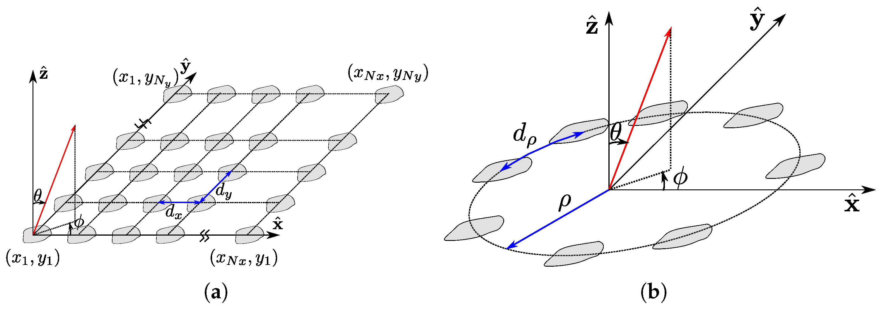
2. Formulation of an Array Pattern Through Hermitian Matrices

This section introduces the use of Hermitian matrices in the formulation of radiation patterns for array antennas to cast a convex problem.

2.1. Directivity of an Array Antenna

The directivity of an antenna can be defined as its ability to concentrate energy in a specific direction in preference to radiation in other directions, which can be determined as the ratio between the radiation intensity U in a given direction $(\theta ,\varphi )$ and the average radiation intensity $U_{\mathrm{ave}}$ as:

$$D\left(\theta ,\varphi \right)={\displaystyle \frac{U\left(\theta ,\varphi \right)}{U_{\mathrm{ave}}}}$$

(1)

Radiation intensity is defined as the power radiated in a given direction per unit solid angle, and it can be related with the total power radiated $P_r$ by an antenna by integrating U over all angles around the antenna, resulting in the following expression

$$P_r={∯}_{\Omega }U\left(\theta ,\varphi \right)d\Omega$$

(2)

where $d\Omega$ is equal to the element of the solid angle defined as $d\Omega =sin\theta d\theta d\varphi$.

Given that the total solid angle in space is $4\pi$ steradian (sr), the radiation intensity of a nonisotropic source, such as an antenna array, is not uniformly distributed. However, an average power per steradian can be defined to characterize the overall spatial distribution as

$$U_{\mathrm{ave}}={\displaystyle \frac{1}{4\pi }}{∯}_{\Omega }U\left(\theta ,\varphi \right)d\Omega ={\displaystyle \frac{P_r}{4\pi }}$$

(3)

Now, replacing (3) in (1), the directivity can be computed as

$${\displaystyle D\left(\theta ,\varphi \right)=\frac{U\left(\theta ,\varphi \right)}{{\displaystyle \frac{1}{4\pi }{∯}_{\Omega }U\left(\theta ,\varphi \right)d\Omega }}=4\pi \frac{U\left(\theta ,\varphi \right)}{P_r}}$$

(4)

At this point, it is necessary to work on (4), as we need to relate directivity to array variables that can be used as degrees of freedom in the optimization process. To achieve this, we start from the definition of the time-averaged value of the Poynting vector defined as:

$${\displaystyle <\overrightarrow{S}>=\frac{1}{2}\Re \{\overrightarrow{E}\times {\overrightarrow{H}}^{\ast }\}}$$

(5)

where $\overrightarrow{E}$ is the electric field, and $\overrightarrow{H}$ is the magnetic field in the frequency domain.

From Poynting’s theorem, the total radiated power of an antenna $\left(P_r\right)$ can be obtained from the surface integral of $<\overrightarrow{S}>$ within the surface aperture ($\Omega$) because the electromagnetic fields outside the antenna are purely radiative. Mathematically:

$$P_r={∯}_{\Omega }<\overrightarrow{S}>·\widehat{n}d\Omega$$

(6)

where $\widehat{n}$ is the unit normal vector outward from the surface, in this case, $\widehat{r}$, by considering a spherical surface.

Thus, $P_r$ comes directly from the integration of the Poynting vector over the surface, encapsulating the radiated energy. Considering that the contributions to the $\widehat{r}$-component of $<\overrightarrow{S}>$ from the electric field $\overrightarrow{E}$ and magnetic field $\overrightarrow{H}$ are solely due to their angular components, they can be written as:

$$\begin{array}{cc}\overrightarrow{E}& =E_{\theta }\widehat{\theta }+E_{\varphi }\widehat{\varphi }\\ \overrightarrow{H}& =H_{\theta }\widehat{\theta }+H_{\varphi }\widehat{\varphi }\end{array}$$

(7)

Both equations in Equation (7) can be related with the plane wave relation in the far-field

$$\overrightarrow{H}={\displaystyle \frac{1}{\eta }}\widehat{r}\times \overrightarrow{E}$$

(8)

where $\eta$ is the characteristic impedance of the propagation medium, in this case air $(\eta =120\pi )$.

Establishing the following relationship between components

$$\begin{array}{cc}{H}_{\varphi }& ={\displaystyle \frac{E_{\theta }}{\eta }}\\ H_{\theta }& =-{\displaystyle \frac{E_{\varphi }}{\eta }}\end{array}$$

(9)

$P_r$ can be expressed as

$$P_r={\displaystyle \frac{1}{2\eta }}{∯}_{\Omega }\left({|E_{\theta }|}^2+{|E_{\varphi }|}^2\right)r^{2}d\Omega ={\displaystyle \frac{1}{2\eta }}{∯}_{\Omega }{|\overrightarrow{E}|}^2{r}^{2}d\Omega$$

(10)

From (2), (5) and (10), $U(\theta ,\varphi )$ can be written as

$$U(\theta ,\varphi )={\displaystyle \frac{1}{2}}\Re \{\overrightarrow{E}\times {\overrightarrow{H}}^{\ast }\}·r^2\widehat{r}={\displaystyle \frac{1}{2\eta }}{|\overrightarrow{E}|}^2{r}^2$$

(11)

Hence, the directivity can now be expressed as

$$D(\theta ,\varphi )={\displaystyle \frac{4\pi |\overrightarrow{E}{(\theta ,\varphi )|}^2}{{\displaystyle {∯}_{\Omega }{|\overrightarrow{E}|}^{2}sin\theta d\theta d\varphi }}}$$

(12)

where $sin\theta$ appears because of the solid angle $d\Omega =sin\theta d\theta d\varphi$.

2.2. Radiation Performance Using Hermitian Forms

The most common goals of array optimization are to maximize directivity in a specific spatial direction [10], reduce the level of sidelobes [24], or create nulls at certain angular positions [26]. To achieve this, in this work, we use a two-dimensional array defined in the x–y plane with radiation in the z-direction $(z>0)$. Figure 1 shows a generic array with $N_x$ and $N_y$ elements along the x- and y-directions, respectively. In this work, we consider two common arrangements for the antenna elements: the element spacing is uniform and they can be distributed in a rectangular regular grid of periodicity $d_x$ and $d_y$ (see Figure 1a), or along a circular arc of radius $\rho$ and distance between elements $d_{\rho }$ (see Figure 1b). However, the formulations presented in this work is applicable to arbitrarily positioned elements (i.e., irregularly spaced arrays).

In addition, in this work, we assume a scalar representation of the radiation pattern of the antenna array, where only the copolar component is considered. The scalar notation is used from this point onward. The radiation pattern is expressed as the product of the elemental radiation pattern $E_e(\theta ,\varphi )$ and the array factor $AF(\theta ,\varphi )$. Therefore, the radiation pattern can now be expressed as

$$E(\theta ,\varphi )=E_e(\theta ,\varphi )·AF(\theta ,\varphi )$$

(13)

The array factor represents the influence of both the element excitations and their spatial arrangement. It is defined as the weighted sum of the contributions from each individual element, each modulated by its complex excitation and the phase shift arising from its position. The array factor is given by

$$AF(\theta ,\varphi )=\sum _{n=1}^N{a}_n{e}^{jk\left({\overrightarrow{r}}_n·\widehat{u}(\theta ,\varphi )\right)}$$

(14)

where N is the total number of elements in the array, $a_n$ is the complex excitation of the nth element, k is the free-space wavenumber, ${\overrightarrow{r}}_n=x_n\widehat{x}+y_n\widehat{y}$ denotes the position vector of the nth element referred to the origin of coordinates, and $\widehat{u}(\theta ,\varphi )$ is the unit vector defined as

$$\widehat{u}(\theta ,\varphi )=sin\theta cos\varphi \widehat{x}+sin\theta sin\varphi \widehat{y}$$

(15)

We can now define the steering vector, which establishes the phase shift of each element, as

$$\overrightarrow{d}(\theta ,\varphi )=\left[\begin{array}{c}{e}^{-jk{\overrightarrow{r}}_1·\widehat{u}(\theta ,\varphi )}\\ e^{-jk{\overrightarrow{r}}_2·\widehat{u}(\theta ,\varphi )}\\ ⋮\\ e^{-jk{\overrightarrow{r}}_N·\widehat{u}(\theta ,\varphi )}\end{array}\right]$$

(16)

while the excitation of the elements can be arranged in vector form as

$$\overrightarrow{a}=\left[\begin{array}{c}{a}_1\\ a_2\\ ⋮\\ a_N\end{array}\right]$$

(17)

so that the array factor can be succinctly expressed as

$$AF(\theta ,\varphi )=\overrightarrow{d}{\left(\theta ,\varphi \right)}^{†}\overrightarrow{a}$$

(18)

where ${\overrightarrow{d}}^{†}$ is the Hermitian conjugate of $\overrightarrow{d}$, which is obtained by taking the transpose of $\overrightarrow{d}$ and then applying complex conjugation to each element.

Considering that the elements are isotropic, $E_e(\theta ,\varphi )=1$, the radiated electric field only depends on the array factor (13)

$$E(\theta ,\varphi )=AF(\theta ,\varphi )$$

(19)

Then, inserting (19) in (12), the directivity at the direction of maximum directivity given by $\left({\theta }_0,{\varphi }_0\right)$ can be written as

$$D({\theta }_0,{\varphi }_0)={\displaystyle \frac{4\pi |E({\theta }_0,{\varphi }_0){|}^2}{{\displaystyle {∯}_S{|E(\theta ,\varphi )|}^{2}sin\theta d\theta d\varphi }}}={\displaystyle \frac{4\pi |AF({\theta }_0,{\varphi }_0){|}^2}{{\displaystyle {∯}_S{|AF(\theta ,\varphi )|}^{2}sin\theta d\theta d\varphi }}}$$

(20)

According to (18), the array factor can be expressed through the steering vector $\overrightarrow{d}(\theta ,\varphi )$ and the complex excitation vector $\overrightarrow{a}$. Since $\overrightarrow{a}\in {\mathbb{C}}^{N\times 1}$, $\overrightarrow{d}(\theta ,\varphi )\in {\mathbb{C}}^{N\times 1}$, $\overrightarrow{d}{(\theta ,\varphi )}^{†}\in {\mathbb{C}}^{1\times N}$, and ${\overrightarrow{a}}^{†}\in {\mathbb{C}}^{1\times N}$, the squared absolute value of the array factor ${|AF(\theta ,\varphi )|}^2$ can be computed as

$${|E(\theta ,\varphi )|}^2={|AF(\theta ,\varphi )|}^2={|\overrightarrow{d}{\left(\theta ,\varphi \right)}^{†}\overrightarrow{a}|}^2={\overrightarrow{a}}^{†}\overrightarrow{d}\left(\theta ,\varphi \right)\overrightarrow{d}{\left(\theta ,\varphi \right)}^{†}\overrightarrow{a}$$

(21)

This expression has been rewritten using the associative property of matrix multiplication to obtain the product $\overrightarrow{d}(\theta ,\varphi )\overrightarrow{d}{(\theta ,\varphi )}^{†}$, which defines a rank-one Hermitian matrix $\mathbf{Q}(\theta ,\varphi )$. This allows us to express the array factor as a Hermitian form ([32], Ch. X), which is widely used in array synthesis and optimization problems due to its convex properties that guarantee achieving the best global maximum value [13].

$${|E(\theta ,\varphi )|}^2={|AF(\theta ,\varphi )|}^2={\overrightarrow{a}}^{†}\mathbf{Q}(\theta ,\varphi )\overrightarrow{a}$$

(22)

where $\mathbf{Q}(\theta ,\varphi )\in {\mathbb{C}}^{N\times N}$.

Then, the directivity (20) is written as

$$D({\theta }_0,{\varphi }_0)={\displaystyle \frac{4\pi \left[{\overrightarrow{a}}^{†}\mathbf{Q}({\theta }_0,{\varphi }_0)\overrightarrow{a}\right]}{{\displaystyle {∯}_S{\overrightarrow{a}}^{†}\mathbf{Q}(\theta ,\varphi )\overrightarrow{a}sin\theta d\theta d\varphi }}}={\displaystyle \frac{4\pi \left[{\overrightarrow{a}}^{†}\mathbf{Q}\left({\theta }_0,{\varphi }_0\right)\overrightarrow{a}\right]}{{\overrightarrow{a}}^{†}\left({\displaystyle {∯}_S\mathbf{Q}(\theta ,\varphi )sin\theta d\theta d\varphi }\right)\overrightarrow{a}}}={\displaystyle \frac{4\pi \left[{\overrightarrow{a}}^{†}{\mathbf{Q}}_0\overrightarrow{a}\right]}{{\overrightarrow{a}}^{†}\mathbf{P}\overrightarrow{a}}}$$

(23)

where $\mathbf{P}$ is the average matrix of the radiated field distribution throughout space, and ${\mathbf{Q}}_0$ is the Hermitian matrix $\mathbf{Q}$ when $\left(\theta ,\varphi \right)$ is $\left({\theta }_0,{\varphi }_0\right)$.

This expression of the directivity is the key point for convex optimization, as it allows us to optimize directivity through the ratio of the Hermitian forms given by ${\overrightarrow{a}}^{†}{\mathbf{Q}}_0\overrightarrow{a}$ and ${\overrightarrow{a}}^{†}\mathbf{P}\overrightarrow{a}$, with the excitation vector $\overrightarrow{a}$, which are the optimization variables. The total radiated power of the array is calculated with $\mathbf{P}$, which is obtained by integrating $\mathbf{Q}(\theta ,\varphi )$ over the entire radiation sphere. $\mathbf{Q}(\theta ,\varphi )$ represents the contribution of the array factor in a given direction $(\theta ,\varphi )$, and is derived from the product $(\overrightarrow{d}{\overrightarrow{d}}^{†})$, ensuring that $\mathbf{Q}(\theta ,\varphi )$ is Hermitian and positive definite. The integral in (23) aggregates these contributions over all directions, resulting in a matrix with the total radiated power. Since the array radiates power for any nonzero excitation vector $\overrightarrow{a}$, the total radiated power in (23) must be strictly positive for any $\overrightarrow{a}\ne 0$, which implies that $\mathbf{P}$ is also positive definite. Furthermore, because $\mathbf{Q}(\theta ,\varphi )$ is positive definite, all its eigenvalues are strictly positive, ensuring that it is also nonsingular. Therefore, the Hermitian form in (23) remains well posed and allows for its use in convex optimization.

Now, the maximization of directivity can be recast as the maximization of the Rayleigh quotient [13]

$${\displaystyle \underset{\overrightarrow{a}}{max}\left\{\frac{{\overrightarrow{a}}^{†}{\mathbf{Q}}_0\overrightarrow{a}}{{\overrightarrow{a}}^{†}\mathbf{P}\overrightarrow{a}}\right\}}$$

(24)

This optimization is equivalent to solving the generalized eigenvalue problem

$${\mathbf{Q}}_0\overrightarrow{a}=\lambda \mathbf{P}\overrightarrow{a}$$

(25)

where the maximum directivity is the maximum value of the Rayleigh quotient, which corresponds to the largest eigenvalue ${\lambda }_{\max }$, and the optimal excitation vector ${\overrightarrow{a}}_{\mathrm{opt}}$ is given by the associated eigenvector.

2.3. Additional Constraints: Null and Sidelobe Level Control

In practical antenna array design, it is often necessary not only to maximize directivity in a certain direction but also to impose additional constraints to shape the radiation pattern. Specifically, usual constraints are aimed at enforcing nulls and controlling the SLLs. These constraints are essential to mitigate interference in specific directions and ensure that all the radiated power is focused on the intended directions.

The objective is now to reach maximum directivity towards $({\theta }_0,{\varphi }_0)$ but also to impose nulls in specific directions $({\theta }_q,{\varphi }_q)$. To do so, it is required that the radiation intensity is null in those directions, which can be mathematically expressed as the following equality constraint

$${\overrightarrow{a}}^{†}{\mathbf{Q}}_q\overrightarrow{a}=0\forall ({\theta }_q,{\varphi }_q)\in \mathcal{Q}$$

(26)

where ${\mathbf{Q}}_q$ is $\mathbf{Q}(\theta ,\varphi )$ evaluated at $\left({\theta }_q,{\varphi }_q\right)$, which are the angle directions within a $\mathcal{Q}$ set wherein the null requirements are imposed.

Similarly, to limit the sidelobe levels, it is feasible to impose constraints on a certain region where the SLLs must be controlled. This means that the radiation intensity must be below a certain threshold, and it can be formulated as

$${\overrightarrow{a}}^{†}{\mathbf{Q}}_m\overrightarrow{a}\le {\xi }_m\forall ({\theta }_m,{\varphi }_m)\in \mathcal{M}$$

(27)

where $\xi$ is the maximum allowable power level in the sidelobe region, ${\mathbf{Q}}_m$ is the matrix $\mathbf{Q}(\theta ,\varphi )$ evaluated at $\left({\theta }_m,{\varphi }_m\right)$, which are the angle directions defined within an $\mathcal{M}$ set (usually corresponding to discretized sidelobe regions) wherein the SLL restrictions are imposed.

This condition ensures that the power radiated by the array outside the main lobe remains below the threshold, thereby controlling spurious radiation towards undesired directions and improving overall pattern performance.

The Rayleigh quotient in (24) can now be rewritten as a constrained problem:

$$\begin{array}{cc}\hfill \underset{\overrightarrow{a}}{max}& \left\{{\displaystyle \frac{{\overrightarrow{a}}^{†}{\mathbf{Q}}_0\overrightarrow{a}}{{\overrightarrow{a}}^{†}\mathbf{P}\overrightarrow{a}}}\right\}\hfill \\ \hfill & \mathrm{subject}\mathrm{to}{\overrightarrow{a}}^{†}\mathbf{Q}({\theta }_q,{\varphi }_q)\overrightarrow{a}=0,\forall ({\theta }_q,{\varphi }_q)\in \mathcal{Q}\hfill \\ \hfill & {\overrightarrow{a}}^{†}\mathbf{Q}({\theta }_m,{\varphi }_m)\overrightarrow{a}\le {\xi }_m,\forall ({\theta }_m,{\varphi }_m)\in \mathcal{M}.\hfill \end{array}$$

(28)

Please note that the newly added constraints as Hermitian forms seem to render the problem non-convex. However, by proper manipulations, we can find alternative convex formulations that can be tackled by quadratic programming (QP), second-order cone programming (SOCP) and linear programming (LP).

3. Quadratic Programming

QP allows for the search of the optimal solution by minimizing a quadratic function subject to multiple linear constraints, both inequality and equality constraints. The general expression for quadratic optimization with $N_v$ optimization variables, $N_i$ inequality constraints, and $N_e$ equality constraints is given by

$$\begin{array}{cc}\hfill & \underset{\overrightarrow{x}}{min}{\displaystyle \frac{1}{2}}{\overrightarrow{x}}^T\mathbf{M}\overrightarrow{x}+{\overrightarrow{c}}^T\overrightarrow{x}\hfill \\ \hfill & \mathrm{subject}\mathrm{to}\mathbf{A}\overrightarrow{x}\le \overrightarrow{b}\hfill \\ \hfill & {\mathbf{A}}_{\mathrm{eq}}\overrightarrow{x}={\overrightarrow{b}}_{\mathrm{eq}}\hfill \end{array}$$

(29)

where $\mathbf{M}\in {\mathbb{R}}^{N_v\times N_v}$ is a positive definite matrix containing the coefficients of the quadratic terms, $\overrightarrow{c}\in {\mathbb{R}}^{N_v}$ contains the coefficients of the linear terms, and $\overrightarrow{x}\in {\mathbb{R}}^{N_v}$ is the vector of optimization variables. The matrices $\mathbf{A}\in {\mathbb{R}}^{N_i\times N_v}$ and ${\mathbf{A}}_{\mathrm{eq}}\in {\mathbb{R}}^{N_e\times N_v}$ define the inequality and equality constraints, respectively, with the corresponding right-hand-side vectors $\overrightarrow{b}\in {\mathbb{R}}^{N_i}$ and ${\overrightarrow{b}}_{\mathrm{eq}}\in {\mathbb{R}}^{N_e}$. The specific physical interpretation of these parameters in the context of array optimization is detailed progressively throughout this section.

3.1. QP Formulation for Antenna Array Convex Optimization

From (23), we can derive that radiation intensity needs to be fixed to a certain value, while the minimization of the radiation power directly leads to maximizing the directivity [14]. Therefore, the maximization of the directivity can be expressed as

$$\begin{array}{cc}\hfill & \underset{\overrightarrow{a}}{min}{\overrightarrow{a}}^{†}\mathbf{P}\overrightarrow{a}\hfill \\ \hfill & \mathrm{subject}\mathrm{to}{\overrightarrow{a}}^{†}{\mathbf{Q}}_0\overrightarrow{a}={|\zeta |}^2\hfill \end{array}$$

(30)

where ${|\zeta |}^2$ is taken as the positive real-valued constant to ensure the radiation intensity in the direction of the main beam is fixed.

This problem can be reformulated to be compatible with quadratic programming by modifying the constraint to convert it into a linear constraint. Instead of directly imposing that the radiation intensity must be equal to a constant (positive, real-valued), this requirement can be equivalently expressed in terms of the electric field. That is, we enforce that the electric field must be equal to a specific complex-valued constant. According to (20), since

$$|E({\theta }_0,{\varphi }_0){|}^2={\overrightarrow{a}}^{†}{\mathbf{Q}}_0\overrightarrow{a}={\overrightarrow{a}}^{†}\overrightarrow{d}\left({\theta }_0,{\varphi }_0\right)\overrightarrow{d}{\left({\theta }_0,{\varphi }_0\right)}^{†}\overrightarrow{a}={|\zeta |}^2$$

(31)

$|E({\theta }_0,{\varphi }_0)|$ takes the form

$$|E({\theta }_0,{\varphi }_0)|=|\overrightarrow{d}{\left({\theta }_0,{\varphi }_0\right)}^{†}\overrightarrow{a}|=|\zeta |$$

(32)

Since, as previously stated, the electric field is a complex quantity, this constraint can be decomposed into its real and imaginary components, i.e., $\zeta ={\zeta }_{\mathrm{R}}+j{\zeta }_{\mathrm{I}}$, leading to two independent linear constraints of the form [24]

$$\left\{\begin{array}{c}\Re \left(E({\theta }_0,{\varphi }_0)\right)=\Re \left(\overrightarrow{d}{({\theta }_0,{\varphi }_0)}^{†}\overrightarrow{a}\right)={\zeta }_{\mathrm{R}},\hfill \\ \Im \left(E({\theta }_0,{\varphi }_0)\right)=\Im \left(\overrightarrow{d}{({\theta }_0,{\varphi }_0)}^{†}\overrightarrow{a}\right)={\zeta }_{\mathrm{I}}.\hfill \end{array}\right.$$

(33)

where ${\zeta }_{\mathrm{R}}\mathrm{and}{\zeta }_{\mathrm{I}}\in \mathbb{R}$.

By adopting this formulation, we fix the field magnitude in the desired direction $({\theta }_0,{\varphi }_0)$ and minimize the total radiated power. If the term $\left(\overrightarrow{d}{({\theta }_0,{\varphi }_0)}^{†}\overrightarrow{a}\right)$ is further developed, it can be expressed as

$$\begin{array}{cc}\hfill \overrightarrow{d}{({\theta }_0,{\varphi }_0)}^{†}\overrightarrow{a}& =\left[\Re \left(\overrightarrow{d}{({\theta }_0,{\varphi }_0)}^{†}\right)+j\Im \left(\overrightarrow{d}{({\theta }_0,{\varphi }_0)}^{†}\right)\right]\left[\Re \left(\overrightarrow{a}\right)+j\Im \left(\overrightarrow{a}\right)\right]\hfill \\ \hfill & =\Re \left(\overrightarrow{d}{({\theta }_0,{\varphi }_0)}^{†}\right)\Re \left(\overrightarrow{a}\right)-\Im \left(\overrightarrow{d}{({\theta }_0,{\varphi }_0)}^{†}\right)\Im \left(\overrightarrow{a}\right)\hfill \\ \hfill & +j\left[\Re \left(\overrightarrow{d}{({\theta }_0,{\varphi }_0)}^{†}\right)\Im \left(\overrightarrow{a}\right)+\Im \left(\overrightarrow{d}{({\theta }_0,{\varphi }_0)}^{†}\right)\Re \left(\overrightarrow{a}\right)\right]\hfill \end{array}$$

(34)

Replacing (34) in (33), the restrictions are now defined as

$$\left\{\begin{array}{c}\Re \left(\overrightarrow{d}{({\theta }_0,{\varphi }_0)}^{†}\overrightarrow{a}\right)=\Re \left(\overrightarrow{d}{({\theta }_0,{\varphi }_0)}^{†}\right)\Re \left(\overrightarrow{a}\right)-\Im \left(\overrightarrow{d}{({\theta }_0,{\varphi }_0)}^{†}\right)\Im \left(\overrightarrow{a}\right)={\zeta }_{\mathrm{R}},\hfill \\ \Im \left(\overrightarrow{d}{({\theta }_0,{\varphi }_0)}^{†}\overrightarrow{a}\right)=\Re \left(\overrightarrow{d}{({\theta }_0,{\varphi }_0)}^{†}\right)\Im \left(\overrightarrow{a}\right)+\Im \left(\overrightarrow{d}{({\theta }_0,{\varphi }_0)}^{†}\right)\Re \left(\overrightarrow{a}\right)={\zeta }_{\mathrm{I}}.\hfill \end{array}\right.$$

(35)

Therefore, the real-valued extended vectors from $\overrightarrow{d}{({\theta }_0,{\varphi }_0)}^{†}$ must be defined to encompass the previous result according to

$$\left\{\begin{array}{c}{\overrightarrow{d}}_{0,\mathrm{R}}^{†}=\left[\Re \left(\overrightarrow{d}{({\theta }_0,{\varphi }_0)}^{†}\right),-\Im \left(\overrightarrow{d}{({\theta }_0,{\varphi }_0)}^{†}\right)\right],\hfill \\ {\overrightarrow{d}}_{0,\mathrm{I}}^{†}=\left[\Im \left(\overrightarrow{d}{({\theta }_0,{\varphi }_0)}^{†}\right),+\Re \left(\overrightarrow{d}{({\theta }_0,{\varphi }_0)}^{†}\right)\right].\hfill \end{array}\right.$$

(36)

Consequently, $\overrightarrow{a}$, which contains the optimization variables, can also be decomposed into its real and imaginary parts, leading to the definition of $\overrightarrow{x}\in {\mathbb{R}}^{N_v}$$({\mathbb{R}}^{N_v}={\mathbb{R}}^{2N})$ as

$$\overrightarrow{x}=\left[\begin{array}{c}\Re \left(\overrightarrow{a}\right)\\ \Im \left(\overrightarrow{a}\right)\end{array}\right]$$

(37)

Although the vector $\overrightarrow{x}$ now implies having to find $2N$ optimization variables, these variables are real-valued, while in the case of working with $\overrightarrow{a}$, these variables were complex. Then, following a similar approach with the $P_r$ term, ${\overrightarrow{a}}^{†}\mathbf{P}\overrightarrow{a}$ can be expanded as

$$\begin{array}{cc}\hfill {\overrightarrow{a}}^{†}\mathbf{P}\overrightarrow{a}& =\left(\Re \left({\overrightarrow{a}}^{†}\right)+j\Im \left({\overrightarrow{a}}^{†}\right)\right)\left(\Re \left(\mathbf{P}\right)+j\Im \left(\mathbf{P}\right)\right)\left(\Re \left(\overrightarrow{a}\right)+j\Im \left(\overrightarrow{a}\right)\right)\hfill \\ \hfill & =\Re \left({\overrightarrow{a}}^{†}\right)\Re \left(\mathbf{P}\right)\Re \left(\overrightarrow{a}\right)-\Im \left({\overrightarrow{a}}^{†}\right)\Re \left(\mathbf{P}\right)\Im \left(\overrightarrow{a}\right)\hfill \\ \hfill & -\Re \left({\overrightarrow{a}}^{†}\right)\Im \left(\mathbf{P}\right)\Im \left(\overrightarrow{a}\right)-\Im \left({\overrightarrow{a}}^{†}\right)\Im \left(\mathbf{P}\right)\Re \left(\overrightarrow{a}\right)\hfill \\ \hfill & +j[\Re \left({\overrightarrow{a}}^{†}\right)\Re \left(\mathbf{P}\right)\Im \left(\overrightarrow{a}\right)+\Im \left({\overrightarrow{a}}^{†}\right)\Re \left(\mathbf{P}\right)\Re \left(\overrightarrow{a}\right)\hfill \\ \hfill & -\Im \left({\overrightarrow{a}}^{†}\right)\Im \left(\mathbf{P}\right)\Im \left(\overrightarrow{a}\right)+\Re \left({\overrightarrow{a}}^{†}\right)\Im \left(\mathbf{P}\right)\Re \left(\overrightarrow{a}\right)]\hfill \\ \hfill & =\Re \left({\overrightarrow{a}}^{†}\right)\Re \left(\mathbf{P}\right)\Re \left(\overrightarrow{a}\right)-\Im \left({\overrightarrow{a}}^{†}\right)\Re \left(\mathbf{P}\right)\Im \left(\overrightarrow{a}\right)\hfill \\ \hfill & +j\left[-\Im \left({\overrightarrow{a}}^{†}\right)\Im \left(\mathbf{P}\right)\Im \left(\overrightarrow{a}\right)+\Re \left({\overrightarrow{a}}^{†}\right)\Im \left(\mathbf{P}\right)\Re \left(\overrightarrow{a}\right)\right]\hfill \end{array}$$

(38)

where the terms involving products of $\left(\Im \left({\overrightarrow{a}}^{†}\right)\Im \left(\mathbf{P}\right)\Re \left(\overrightarrow{a}\right)\right)$ and $\left(\Re \left({\overrightarrow{a}}^{†}\right)\Im \left(\mathbf{P}\right)\Im \left(\overrightarrow{a}\right)\right)$, as well as the terms involving $\left(\Re \left({\overrightarrow{a}}^{†}\right)\Re \left(\mathbf{P}\right)\Im \left(\overrightarrow{a}\right)\right)$ and $\left(\Im \left({\overrightarrow{a}}^{†}\right)\Re \left(\mathbf{P}\right)\Re \left(\overrightarrow{a}\right)\right)$, vanish due to the properties of the vectors and matrices involved. Thus,

$$\left\{\begin{array}{c}\Re \left({\overrightarrow{a}}^{†}\mathbf{P}\overrightarrow{a}\right)=\left(\Re \left({\overrightarrow{a}}^{†}\right)\Re \left(\mathbf{P}\right)\Re \left(\overrightarrow{a}\right)\right)-\left(\Im \left({\overrightarrow{a}}^{†}\right)\Re \left(\mathbf{P}\right)\Im \left(\overrightarrow{a}\right)\right)\hfill \\ \Im \left({\overrightarrow{a}}^{†}\mathbf{P}\overrightarrow{a}\right)=\left(\Re \left({\overrightarrow{a}}^{†}\right)\Im \left(\mathbf{P}\right)\Re \left(\overrightarrow{a}\right)\right)-\left(\Im \left({\overrightarrow{a}}^{†}\right)\Im \left(\mathbf{P}\right)\Im \left(\overrightarrow{a}\right)\right).\hfill \end{array}\right.$$

(39)

Now, the real-valued extended matrices from matrix $\mathbf{P}$ can be set to

$$\left\{\begin{array}{c}{\mathbf{P}}_{\mathrm{R}}=\left[\Re \left(\mathbf{P}\right),-\Re \left(\mathbf{P}\right)\right],\hfill \\ {\mathbf{P}}_{\mathrm{I}}=\left[\Im \left(\mathbf{P}\right),-\Im \left(\mathbf{P}\right)\right].\hfill \end{array}\right.$$

(40)

Therefore, (30) can be reformulated as a quadratic programming problem with linear constraints ($N_e=2$, $N_i=0$) as follows

$$\begin{array}{cc}\hfill & \underset{\overrightarrow{x}}{min}{\overrightarrow{x}}^{†}\left[\begin{array}{c}{\mathbf{P}}_{\mathrm{R}}\\ {\mathbf{P}}_{\mathrm{I}}\end{array}\right]\overrightarrow{x}\hfill \\ \hfill & \mathrm{subject}\mathrm{to}{\overrightarrow{d}}_{0,\mathrm{R}}^{†}\overrightarrow{x}={\zeta }_{\mathrm{R}}\hfill \\ \hfill & {\overrightarrow{d}}_{0,\mathrm{I}}^{†}\overrightarrow{x}={\zeta }_{\mathrm{I}}\hfill \end{array}$$

(41)

where the solution is obtained by

$$\overrightarrow{a}=\left[\begin{array}{c}{x}_1\\ x_2\\ ⋮\\ x_N\end{array}\right]+j\left[\begin{array}{c}{x}_{n+1}\\ x_{n+2}\\ ⋮\\ x_{2N}\end{array}\right]$$

(42)

where $\overrightarrow{a}\in {\mathbb{C}}^N$.

From (41), it can be easily derived that nulls can be set in certain directions. Again, instead of imposing a quadratic constraint for ${\overrightarrow{a}}^{†}\mathbf{Q}\left({\theta }_q,{\varphi }_q\right)\overrightarrow{a}$ to be zero, we can enforce the field to be null in the given direction, expressed as

$$E({\theta }_q,{\varphi }_q)=0$$

(43)

This is equivalent to imposing an additional equality condition in (41), but first, we need to define the steering vector (16) associated with the nulls as

$$\overrightarrow{d}\left({\theta }_q,{\varphi }_q\right)=\left[\begin{array}{c}{e}^{-jk{\overrightarrow{r}}_1·\overrightarrow{u}({\theta }_q,{\varphi }_q)}\\ e^{-jk{\overrightarrow{r}}_2·\overrightarrow{u}({\theta }_q,{\varphi }_q)}\\ ⋮\\ e^{-jk{\overrightarrow{r}}_N·\overrightarrow{u}({\theta }_q,{\varphi }_q)}\end{array}\right]$$

(44)

Following the same procedure as in (36), the null-steering vector $\overrightarrow{d}({\theta }_q,{\varphi }_q)$ can also be decomposed into a real and imaginary part:

$$\left\{\begin{array}{c}{\overrightarrow{d}}_{\mathrm{q},\mathrm{R}}^{†}=\left[\Re \left(\overrightarrow{d}{\left({\theta }_q,{\varphi }_q\right)}^{†}\right),-\Im \left(\overrightarrow{d}{\left({\theta }_q,{\varphi }_q\right)}^{†}\right)\right],\hfill \\ {\overrightarrow{d}}_{\mathrm{q},\mathrm{I}}^{†}=\left[\Im \left(\overrightarrow{d}{\left({\theta }_q,{\varphi }_q\right)}^{†}\right),+\Re \left(\overrightarrow{d}{\left({\theta }_q,{\varphi }_q\right)}^{†}\right)\right].\hfill \end{array}\right.$$

(45)

Now, (41) is modified to be defined as

$$\begin{array}{cc}\hfill & \underset{\overrightarrow{x}}{min}{\overrightarrow{x}}^{†}\left[\begin{array}{c}{\mathbf{P}}_{\mathrm{R}}\\ {\mathbf{P}}_{\mathrm{I}}\end{array}\right]\overrightarrow{x}\hfill \\ \hfill & \mathrm{subject}\mathrm{to}{\overrightarrow{d}}_{0,\mathrm{R}}^{†}\overrightarrow{x}={\zeta }_{\mathrm{R}}\hfill \\ \hfill & {\overrightarrow{d}}_{0,\mathrm{I}}^{†}\overrightarrow{x}={\zeta }_{\mathrm{I}}\hfill \\ \hfill & {\overrightarrow{d}}_{q,\mathrm{R}}^{†}\overrightarrow{x}=0\hfill \\ \hfill & {\overrightarrow{d}}_{q,\mathrm{I}}^{†}\overrightarrow{x}=0\hfill \end{array}$$

(46)

which is a QP problem with $N_i=0$ and $N_e=2+2\dim \left(\mathcal{Q}\right)$. Please note that (41) and (46) are QP problems which only contain equality constraints (i.e., $N_i=0$). In this particular case, there exists a direct solution, as given in [22,30], without the need to resort to an iterative algorithm.

One could think that the addition of inequality constraints to this QP formulation could lead to the inclusion of restrictions in the SLLs. However, this is only possible under certain symmetry conditions in both the array layout and the excitation distribution, correspondingly resulting in array factor symmetries, which render the problem completely real-valued from its inception, as presented in [14]. Since in this paper, we present a more general case to be tackled by SOCP, we limit ourselves to the optimization problems presented in (41) and (46).

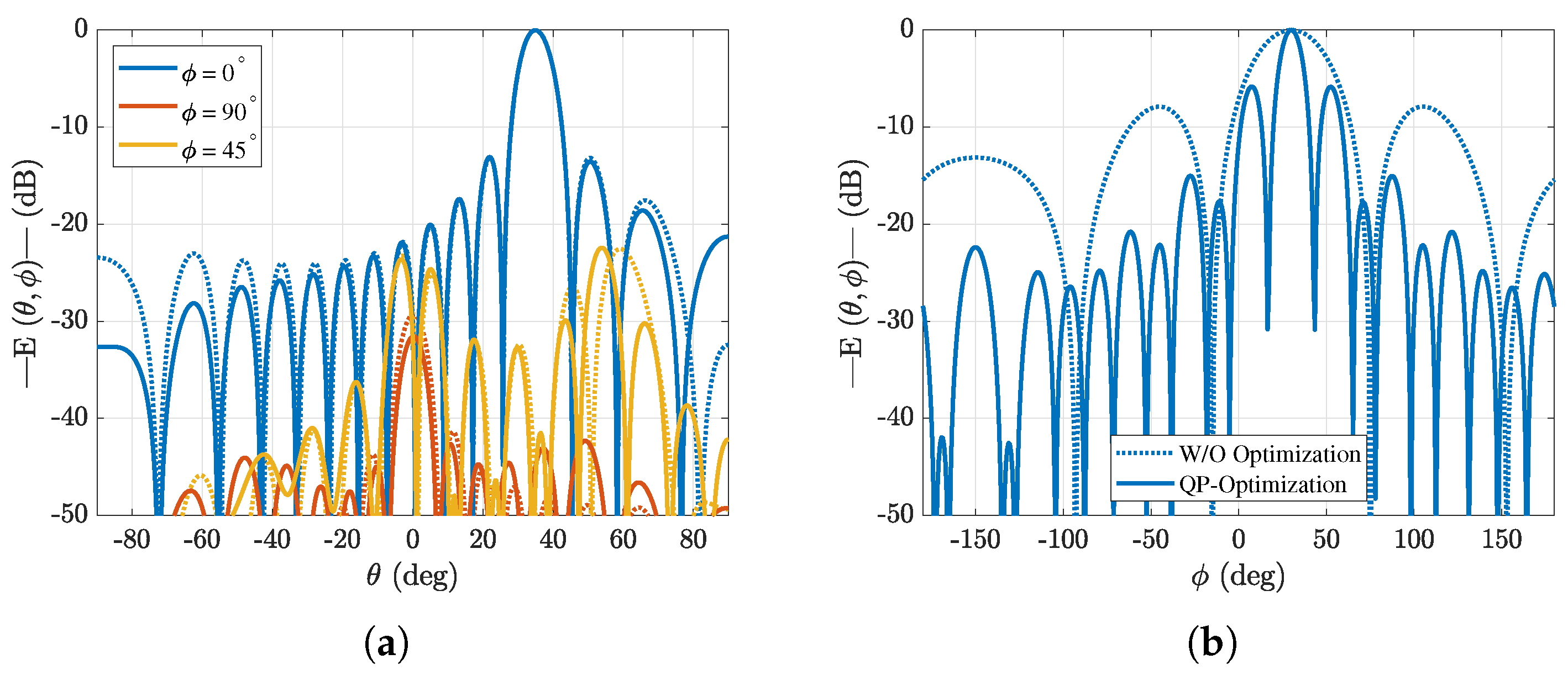
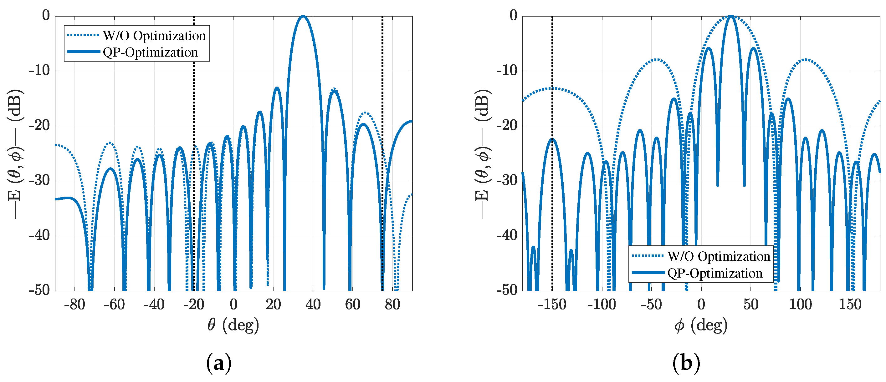
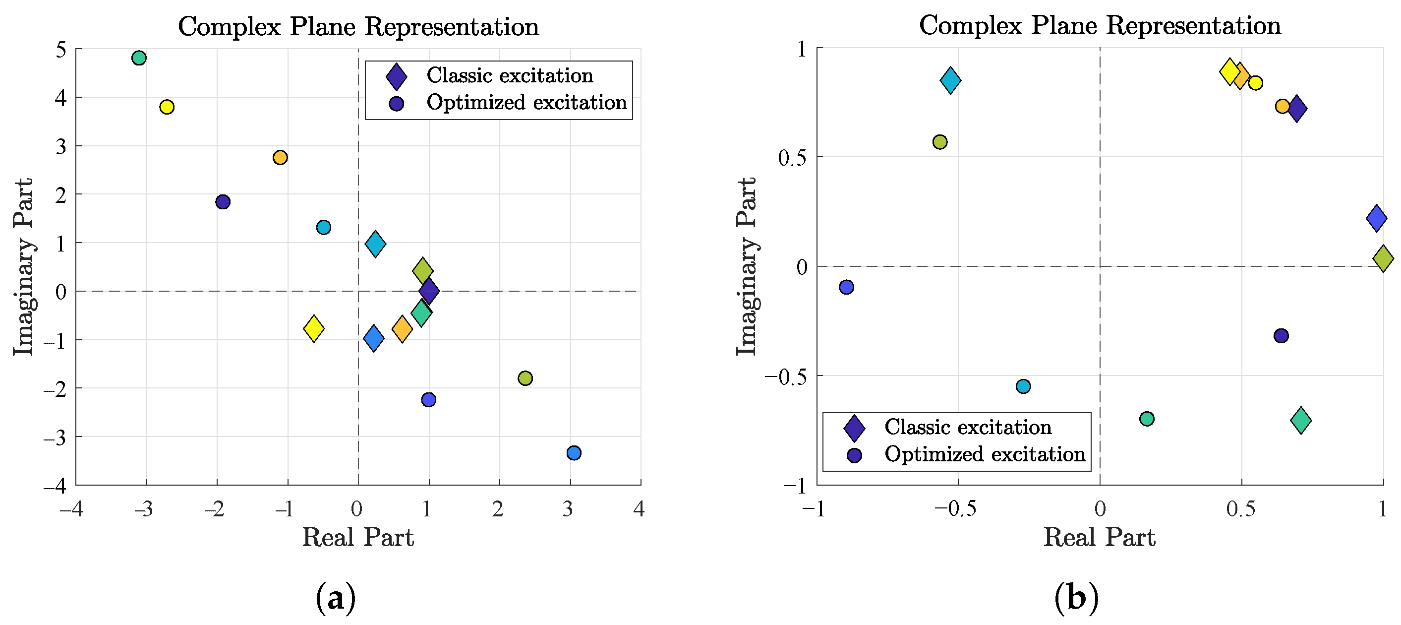
3.2. Results for Optimal Directivity with Null Requirements

Now that the QP formulation for convex optimization has been developed, it is validated through several numerical examples. First, the directivity of an array is maximized to evaluate its improvement compared to an unoptimized design. In a second example, directivity maximization is performed while enforcing null constraints, representing the most complex case that QP allows. Both cases are analyzed for two different array geometries: square and circular.

The array geometry was defined by a configuration of $16\times 16$ elements arranged in a regular square grid, as shown in Figure 1a. The element spacing was set to $0.3{\lambda }_0$, where ${\lambda }_0$ stands for the free-space wavelength at the operating frequency. Additionally, following the developed formulation, the elements were considered isotropic. For the circular array, the configuration consisted of 32 elements with an inter-element radial spacing of $d_{\rho }=0.9{\lambda }_0$ and a radius of $\rho =5{\lambda }_0$ arranged according to the distribution shown in Figure 1b. Note that for the radiation pattern calculations, the array factor (AF) were computed to be equal for both square and circular arrays since, in the case of isotropic elements, the radiated field is proportional to the AF (13). Furthermore, according to (14), the vector ${\overrightarrow{r}}_n$ defined the position of the elements in the x–y plane, eliminating the need for modifications between the circular and square arrays. Additionally, the pointing direction for the square array was set to ${\theta }_0={30}^{\circ }$ and $\varphi =0^{\circ }$, while for the circular array, it was set to ${\theta }_0={90}^{\circ }$ and $\varphi ={30}^{\circ }$. The optimization cases were compared with the results provided by classic excitation to achieve maximum directivity, with the corresponding phase values adjusted to achieve the desired beam steering, i.e., $\overrightarrow{a}=\overrightarrow{d}({\theta }_0,{\varphi }_0)$.

To solve the QP-based optimization, a convex interior-point method was used, although a direct solution [22,30] could be directly implemented. Figure 2 compares the results of the normalized radiation pattern using classic excitations and the excitations obtained from the QP optimization for both arrays. In the case of the square array, the classic excitation provided a very good analytical solution, close to maximum directivity. When the weights were optimized, the resulting radiation pattern remained almost the same, with only slight variations in the SLL level in certain regions. Additionally, besides the main cut ($\varphi =0^{\circ }$), the orthogonal cut ($\varphi ={90}^{\circ }$) and the diagonal cut ($\varphi ={45}^{\circ }$) were evaluated, resulting in a very similar radiation pattern between both excitations. The effect of the optimization was more evident in the case of the circular array, where the classic excitation did not yield a maximum directivity solution. In that case, the optimized weights achieved a much more directive radiation pattern, significantly reducing the main beamwidth and obtaining an SLL distribution much closer to a directive pattern.

Although the classic excitations for the square array already provided a maximum directivity solution, it did not allow enforcing nulls in specific directions. Therefore, it was necessary to use optimization techniques, such as the one proposed in this work, to incorporate additional constraints in the array design. In Figure 3, the same optimization was repeated for both arrays, but with enforced nulls in directions ${\theta }_1=-{20}^{\circ }$ and ${\theta }_2={70}^{\circ }$ for the square array, and at ${\varphi }_1=-{150}^{\circ }$ for the circular array. In both cases, the results were similar to those obtained in Figure 2 but showing a field drop (null) in the specified directions. These results demonstrate that, although analytical solutions provide good directivity performance, when radiation patterns with additional constraints are required, optimization techniques must be employed. In this context, convex optimization with QP programming offers a powerful alternative.

Figure 4 presents the excitation of 10 elements from each array, both before and after optimization, illustrating how the feeding coefficients are clearly modified to generate the desired radiation pattern. Additionally, it highlights how the final solution vector consists of complex-valued elements. These results correspond to the case of directivity maximization with enforced nulls, as it represents the most restrictive scenario.

4. Second-Order Cone Programming

This subsection develops the use of SOCP for radiation pattern optimization to maximize directivity in a given direction while also incorporating constraints for nulls in specific directions and limiting the SLLs in given regions. This involves minimizing a linear function subject to second-order (quadratic) constraints, which can be generally expressed as follows:

$$\begin{array}{cc}\hfill & \underset{\overrightarrow{y}}{min}{\overrightarrow{f}}^T\overrightarrow{y}\hfill \\ \hfill & \mathrm{subject}\mathrm{to}\parallel {\mathbf{A}}_m\overrightarrow{y}+{\overrightarrow{b}}_m\parallel \le {\overrightarrow{c}}_m^T\overrightarrow{y}+d_m,m=1,\dots ,N_i\hfill \\ \hfill & {\mathbf{A}}_{\mathrm{eq}}\overrightarrow{y}={\overrightarrow{b}}_{\mathrm{eq}}\hfill \end{array}$$

(47)

where $N_i$ is the total number of second-order cone inequality constraints, $\overrightarrow{y}\in {\mathbb{R}}^{N_v}$ is the real-valued vector containing the optimization variables, $\overrightarrow{f}\in {\mathbb{R}}^{N_v}$ is the real-valued vector of coefficients for the objective function (analogous to the $\overrightarrow{c}$ in QP), and for each m, the parameters are the real-valued matrix ${\mathbf{A}}_m$, the real-valued vectors ${\overrightarrow{b}}_m$, ${\overrightarrow{c}}_m$ and the scalar $d_m$, which define the affine mapping for the second-order cone inequality constraints. These constraints extend the linear inequality constraints $\mathbf{A}\overrightarrow{y}\le \overrightarrow{b}$ found in QP by incorporating norms. Furthermore, the equality constraints are given by ${\mathbf{A}}_{\mathrm{eq}}\overrightarrow{y}={\overrightarrow{b}}_{\mathrm{eq}}$, which are similar to the QP formulation.

The standard unit second-order convex cone, also referred to as the Lorentz quadratic cone, of dimension k is defined as

$$C_k=\left\{\left[\begin{array}{c}\overrightarrow{u}\\ t\end{array}\right]\in {\mathbb{R}}^k\mid \overrightarrow{u}\in {\mathbb{R}}^{k-1},t\in \mathbb{R},\parallel \overrightarrow{u}\parallel \le t\right\}.$$

(48)

For the particular case where $k=1$, the second-order cone reduces to

$$C_1=\{t\in \mathbb{R}\mid t\ge 0\}.$$

(49)

The set of points satisfying a second-order cone constraint corresponds to the inverse image of the unit second-order cone under an affine mapping:

$$\parallel {\mathbf{A}}_m\overrightarrow{y}+{\overrightarrow{b}}_m\parallel \le {\overrightarrow{c}}_m^T\overrightarrow{y}+d_m⟺\left[\begin{array}{c}{\mathbf{A}}_m\\ {\overrightarrow{c}}_m^T\end{array}\right]\overrightarrow{y}+\left[\begin{array}{c}{\overrightarrow{b}}_m\\ d_m\end{array}\right]\in C_{n_m}.$$

(50)

where $C_{n_m}$ is the dimension of the second-order cone associated with the mth constraint.

Since the second-order cone is convex, it follows that SOCP is a convex optimization problem, with both a convex objective function and convex constraints. Its development was motivated by the quadratic programming formulation by suitably transforming the quadratic term into an equivalent norm constraint.

4.1. SOCP Formulation for Antenna Array Optimization

The resolution of the directivity maximization using SOCP starts from the function for QP in (30), where the goal is to minimize ${\overrightarrow{a}}^{†}\mathbf{P}\overrightarrow{a}$. However, a series of transformations must be applied to this function to make it suitable for SOCP. Considering that the matrix $\mathbf{P}$ can be decomposed into two submatrices such that

$${\overrightarrow{a}}^{†}\mathbf{P}\overrightarrow{a}={\overrightarrow{a}}^{†}{\mathbf{G}}^{†}\mathbf{G}\overrightarrow{a}={\parallel \mathbf{G}\overrightarrow{a}\parallel }^2$$

(51)

where in general, $\mathbf{G}$ could be a rectangular matrix, and $\parallel ·\parallel$ represents the Euclidean norm ${𝓁}_2$ (for further details refer to Appendix A). Actually, since $\mathbf{P}$ is positive definite, it has a Cholesky decomposition such that $\mathbf{P}={\mathbf{G}}^{†}\mathbf{G}$.

According to Appendix B, minimizing the squared norm is equivalent to minimizing the norm itself. Therefore, the cost function can be reformulated as a norm function that can be directly handled by SOCP, leading to the following minimization problem:

$$\begin{array}{cc}\hfill & \underset{\overrightarrow{a}}{min}\parallel \mathbf{G}\overrightarrow{a}\parallel \hfill \\ \hfill \mathrm{subject}\mathrm{to}& {\overrightarrow{a}}^{†}{\mathbf{Q}}_0\overrightarrow{a}={|\zeta |}^2\hfill \end{array}$$

(52)

As it happened in QP, both $\overrightarrow{a}$ and $\mathbf{G}$ belong to the field of complex numbers and, therefore, can be decomposed to express the norm from their real and imaginary parts, generating the following minimization function.

$$\begin{array}{cc}\hfill & \underset{\overrightarrow{x}}{min}∥\left[\begin{array}{c}{\mathbf{G}}_{\mathrm{R}}\\ {\mathbf{G}}_{\mathrm{I}}\end{array}\right]\overrightarrow{x}∥\hfill \\ \hfill & \mathrm{subject}\mathrm{to}{\overrightarrow{d}}_{0,\mathrm{R}}^{†}\overrightarrow{x}={\zeta }_{\mathrm{R}}\hfill \\ \hfill & {{\overrightarrow{d}}_{0,\mathrm{I}}}^{†}\overrightarrow{x}={\zeta }_{\mathrm{I}}\hfill \end{array}$$

(53)

where $\overrightarrow{x}\in {\mathbb{R}}^{2N}$ (according to (37), $\overrightarrow{x}=\left[\begin{array}{c}\Re \left(\overrightarrow{a}\right)\\ \Im \left(\overrightarrow{a}\right)\end{array}\right]$), and ${\mathbf{G}}_{\mathrm{R}}=\left[\Re \left(\mathbf{G}\right),-\Im \left(\mathbf{G}\right)\right]$ and ${\mathbf{G}}_{\mathrm{I}}=\left[\Im \left(\mathbf{G}\right),+\Re \left(\mathbf{G}\right)\right]$. The equality constraints in (53) are derived in the same manner from the constraint in (52) as in the QP formulation.

This transformation converts the original complex optimization problem into an equivalent real-valued formulation suitable for SOCP. In this reformulated problem, the optimization variable vector $\overrightarrow{x}$ contains the real and imaginary components of the original excitation vector $\overrightarrow{a}$, as in the QP formulation.

In order to fit the SOCP framework, which minimizes a linear objective subject to second-order cone constraints, we introduce an auxiliary scalar variable $\delta$ to serve as an upper bound on the norm of $\mathbf{G}\overrightarrow{a}$. That is, we impose

$$\parallel \mathbf{G}\overrightarrow{a}\parallel \le \delta ,$$

(54)

By minimizing $\delta$, the cost function is effectively reformulated as a linear function, facilitating its handling by SOCP. Therefore, the formulation in (53) can be modified as:

$$\begin{array}{cc}\hfill & \underset{\overrightarrow{x}}{min}\delta \hfill \\ \hfill & \mathrm{subject}\mathrm{to}∥\left[\begin{array}{c}{\mathbf{G}}_{\mathrm{R}}\\ {\mathbf{G}}_{\mathrm{I}}\end{array}\right]\overrightarrow{x}∥\le \delta \hfill \\ \hfill & {\overrightarrow{d}}_{0,\mathrm{R}}^{†}\overrightarrow{x}={\zeta }_{\mathrm{R}}\hfill \\ \hfill & {\overrightarrow{d}}_{0,\mathrm{I}}^{†}\overrightarrow{x}={\zeta }_{\mathrm{I}}\hfill \end{array}$$

(55)

To fully adapt this formulation to SOCP, we need to define $\delta$ as a linear cost function of the optimization variables as follows:

$$\delta ={\overrightarrow{f}}^T\overrightarrow{y},$$

(56)

where $\overrightarrow{f}={[0,0,\dots ,0,1]}^T\in {\mathbb{R}}^{2N+1}$ and $\overrightarrow{y}=\left[\begin{array}{c}\overrightarrow{x}\\ \delta \end{array}\right]\in {\mathbb{R}}^{2N+1}$.

This formulation is consistent with (47), considering that we are now optimizing over $\overrightarrow{y}$ instead of just $\overrightarrow{x}$. Here, $\overrightarrow{y}$ contains the original vector $\overrightarrow{x}$ (formed by the real and imaginary parts of $\overrightarrow{a}$) along with the auxiliary variable $\delta$, yielding a total of $2N+1$ optimization variables. Since $\overrightarrow{f}$ is a vector of zeros except for its last entry, it is entirely appropriate that the cost function minimizes $\delta$ directly. Due to this adjustment in the definition of $\delta$, it is also necessary to modify the submatrices ${\mathbf{G}}_{\mathrm{R}}$ and ${\mathbf{G}}_{\mathrm{I}}$ by appending a column of zeros to each, as follows:

$${\tilde{\mathbf{G}}}_{\mathrm{R}}=\left[\begin{array}{cc}{\mathbf{G}}_{\mathrm{R}}& \mathbf{0}\end{array}\right],{\tilde{\mathbf{G}}}_{\mathrm{I}}=\left[\begin{array}{cc}{\mathbf{G}}_{\mathrm{I}}& \mathbf{0}\end{array}\right].$$

(57)

Similarly, the vectors ${\overrightarrow{d}}_{0,\mathrm{R}}$ and ${\overrightarrow{d}}_{0,\mathrm{I}}$ must be redefined as:

$${\tilde{d}}_{0,\mathrm{R}}=\left[\begin{array}{c}{\overrightarrow{d}}_{0,\mathrm{R}}\\ 0\end{array}\right],{\tilde{d}}_{0,\mathrm{I}}=\left[\begin{array}{c}{\overrightarrow{d}}_{0,\mathrm{I}}\\ 0\end{array}\right].$$

(58)

Now, (55) is rewritten as

$$\begin{array}{cc}\hfill & \underset{\overrightarrow{y}}{min}{\overrightarrow{f}}^T\overrightarrow{y}\hfill \\ \hfill & \mathrm{subject}\mathrm{to}∥\left[\begin{array}{c}{\tilde{\mathbf{G}}}_R\\ {\tilde{\mathbf{G}}}_I\end{array}\right]\overrightarrow{y}∥\le {\overrightarrow{f}}^T\overrightarrow{y}\hfill \\ \hfill & {\tilde{d}}_{0,\mathrm{R}}^{†}\overrightarrow{y}={\zeta }_{\mathrm{R}}\hfill \\ \hfill & {\tilde{d}}_{0,\mathrm{I}}^{†}\overrightarrow{y}={\zeta }_{\mathrm{I}}\hfill \end{array}$$

(59)

where $\overrightarrow{y}$ is the solution of the optimization; however, the variable change involving $\delta$ must be reversed, so the solution of interest is $\overrightarrow{x}=\left\{y_1,y_2,\dots ,y_{2N}\right\}$.

This development enables the optimization of arrays to maximize directivity via SOCP by employing a linearized cost function and quadratic constraints. To include constraints that enforce nulls in specific spatial directions, the same procedure as in QP is followed, since these are linear restrictions compatible with SOCP. However, the minimization of the SLLs in specific directions of the radiation space requires a quadratic constraint, so that within the desired radiation region, the radiated field level is limited to a maximum threshold. Since the SLLs are defined as a relative level with respect to the maximum radiation, this constraint can be expressed as

$$|E({\theta }_m,{\varphi }_m)|\le T_m|E({\theta }_0,{\varphi }_0)|,$$

(60)

where $({\theta }_m,{\varphi }_m)$ are the angle directions that define the region $\mathcal{M}$ in which the SLL conditions are imposed, and $T_m$ is the maximum allowable SLL threshold defined as

$$T_m={10}^{-SL{L}_m/20},$$

(61)

with $SL{L}_m$ representing the desired attenuation (in dB) in the direction $({\theta }_m,{\varphi }_m)$ relative to the maximum radiated field in the direction $({\theta }_0,{\varphi }_0)$.

Given that the field is normalized with respect to the value in the direction $({\theta }_0,{\varphi }_0)$, (60) can be expressed in terms of the excitation vector $\overrightarrow{a}$ and the steering vector as

$$|\overrightarrow{d}{({\theta }_m,{\varphi }_m)}^{†}\overrightarrow{a}|\le T_m\sqrt{{\zeta }_{\mathrm{R}}^2+{\zeta }_{\mathrm{I}}^2},$$

(62)

where $\overrightarrow{d}{({\theta }_m,{\varphi }_m)}^{†}$ is the steering vector in the direction $({\theta }_m,{\varphi }_m)\in \mathcal{M}$, as defined in (44). Then, the magnitude of the radiated field $|E({\theta }_0,{\varphi }_0)|$ results from the fixed values of its real and imaginary parts, ${\zeta }_{\mathrm{R}}$ and ${\zeta }_{\mathrm{I}}$.

Since the operation $|\overrightarrow{d}{({\theta }_m,{\varphi }_m)}^{†}\overrightarrow{a}|$ is equivalent to the Euclidean norm ${𝓁}_2$, one can follow the same procedure as in (33), (32) and (58) to express (62) in terms of its real and imaginary parts, that is,

$$∥\left[\begin{array}{c}{\tilde{d}}_{m,\mathrm{R}}^{†}\\ {\tilde{d}}_{m,\mathrm{I}}^{†}\end{array}\right]\overrightarrow{y}∥\le T_m\sqrt{{\zeta }_{\mathrm{R}}^2+{\zeta }_{\mathrm{I}}^2}.$$

(63)

where ${\tilde{d}}_{m,\mathrm{R}}$ and ${\tilde{d}}_{m,\mathrm{I}}$ is defined as

$${\tilde{d}}_{m,\mathrm{R}}=\left[\begin{array}{c}{\overrightarrow{d}}_{m,\mathrm{R}}\\ 0\end{array}\right],{\tilde{d}}_{m,\mathrm{I}}=\left[\begin{array}{c}{\overrightarrow{d}}_{m,\mathrm{I}}\\ 0\end{array}\right].$$

(64)

Note that this expression is compatible with (59). Finally, the convex optimization problem for maximizing directivity, placing nulls in specific directions, and reducing the SLL level can be formulated as an SOCP problem:

$$\begin{array}{cc}\hfill & \underset{\overrightarrow{y}}{min}{\overrightarrow{f}}^T\overrightarrow{y}\hfill \\ \hfill & \mathrm{subject}\mathrm{to}∥\left[\begin{array}{c}{\tilde{\mathbf{G}}}_{\mathrm{R}}\\ {\tilde{\mathbf{G}}}_{\mathrm{I}}\end{array}\right]\overrightarrow{y}∥\le {\overrightarrow{f}}^T\overrightarrow{y}\hfill \\ \hfill & ∥\left[\begin{array}{c}{\tilde{d}}_{m,\mathrm{R}}^{†}\\ {\tilde{d}}_{m,\mathrm{I}}^{†}\end{array}\right]\overrightarrow{y}∥\le T_m\sqrt{{\zeta }_{\mathrm{R}}^2+{\zeta }_{\mathrm{I}}^2},\forall ({\theta }_m,{\varphi }_m)\in \mathcal{M}\hfill \\ \hfill & {\tilde{d}}_{0,\mathrm{R}}^{†}\overrightarrow{y}={\zeta }_{\mathrm{R}}\hfill \\ \hfill & {\tilde{d}}_{0,\mathrm{I}}^{†}\overrightarrow{y}={\zeta }_{\mathrm{I}}\hfill \\ \hfill & {\tilde{d}}_{\mathrm{q},\mathrm{R}}^{†}\overrightarrow{y}=0,\forall ({\theta }_q,{\varphi }_q)\in \mathcal{Q}\hfill \\ \hfill & {\tilde{d}}_{\mathrm{q},\mathrm{I}}^{†}\overrightarrow{y}=0,\forall ({\theta }_q,{\varphi }_q)\in \mathcal{Q}\hfill \end{array}$$

(65)

Please note that in this SOCP problem, $N_v=2N+1$, $N_e=2+2\dim \left(\mathcal{Q}\right)$ and $N_i=1+\dim \left(\mathcal{M}\right)$.

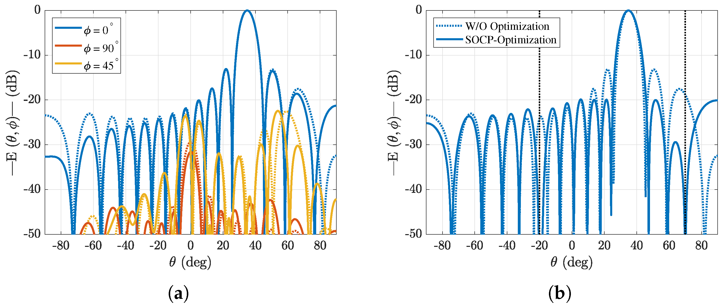
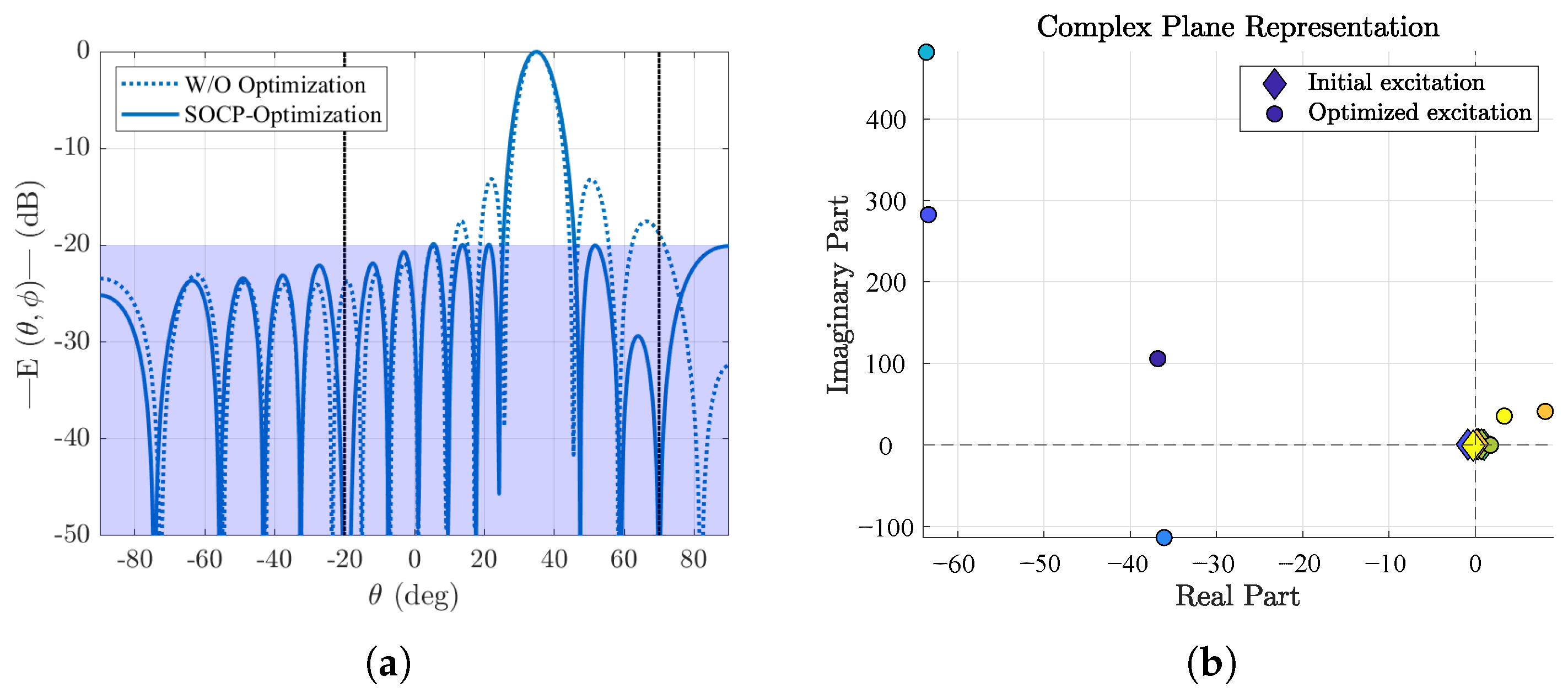
4.2. Results for Optimal Directivity with Different Degrees of Constraints

Taking as a reference the previous square array geometry, three different optimizations were carried out. The first two were analogous to the examples shown for QP, meaning that the first case sought to maximize directivity, while in the second case, that objective was supplemented with the constraint of null generation. For the square array, two nulls were enforced in directions ${\theta }_1=-{20}^{\circ }$ and ${\theta }_2={70}^{\circ }$, while for the circular array, a null was generated at ${\varphi }_1=-{150}^{\circ }$. These cases should have produced results similar to those obtained with QP. However, the third case was exclusive to SOCP, as it involved reducing the SLL level, which required a quadratic constraint (65), while still incorporating the same null generation as in the second case and maximizing directivity in the pointing direction.

Figure 5 shows the radiation pattern for the first two cases, obtaining a result similar to the classic excitation with maximum directivity but enforcing null generation in the second optimization. Similarly, these results closely resemble those obtained with QP. However, the potential of SOCP lies in its ability to incorporate the same constraints as QP while also reducing SLLs. In this example, the SLL levels were relatively low across most of the angular range, but the first sidelobes exceeded $-15$ dB, which may not be optimal for many applications. In the third example, an additional constraint was introduced to set a maximum threshold of $-20$ dB (relative to the maximum) for the SLLs.

Figure 6a presents the radiation pattern using classic excitation and the optimized SOCP solution when combining the three constraints. It can be observed that while maintaining a highly directive beam, not only were two nulls generated in the desired directions, but the SLL level across the entire angular range was also reduced to $-20$ dB. It is important to note that the solution sought to meet the maximum directivity achievable with all requirements established as constraints met, rather than freely maximizing directivity. In the directions of the imposed nulls, regions with a minimum level were generated, while in the rest of the visible range, the SLL levels were maintained at $-20\mathrm{dB}$ relative to the maximum. Therefore, the obtained excitations produced a pattern that met all imposed constraints.

Figure 6b presents eight random samples of the excitations of the classical excitation vector and the SOCP-optimized excitation vector. Due to the imposition of highly complex constraints that impact various aspects of the radiation pattern, the optimized excitations differed significantly from the initial solution, a behavior not observed in QP. In fact, the initial excitations were hardly noticeable, as they remained concentrated around the origin of the complex representation plane, whereas many of the optimized excitations were orders of magnitude larger.

For the circular array, the more complete SOCP optimization was repeated, i.e., including directivity maximization, null forcing, and SLL level reduction. Maintaining the previously defined circular array geometry, the null was imposed in the same directions as in the QP case. Additionally, the SLL level was forced to be reduced to $-10$ dB, $-12$ dB, and $-20$ dB depending on the angular margin selected.

Figure 7 shows the radiation pattern using the classical excitation and the SOCP-based optimized one. These results are particularly promising and demonstrate the potential of the proposed technique. Although QP significantly improved directivity, achieving a much more collimated beam compared to classical excitations, the SLL levels in the first sidelobes remained relatively high, exceeding −10 dB, which is not practical for many applications. The results with SOCP not only showed that a highly directive pattern could be obtained but also that by imposing SLL constraints, the adjacent lobes to the main beam could be drastically reduced, in our case, enforcing drops of −12 dB and −20 dB or −10 dB in more distant regions. Additionally, a null was enforced in the direction $\varphi =-{150}^{\circ }$.

The effect of the optimization can be observed in Figure 8, where the $\theta$–$\varphi$ plane is shown for both the analytical excitations and those obtained with SOCP. These results not only show greater directivity of the main beam but also significantly reduce the level in the rest of the angular space, eliminating radiation in undesired regions. These findings demonstrate how SOCP enables the design of arrays with complex constraints.

5. LP Formulation for SLL Minimization

LP is suitable for addressing optimization problems involving a linear cost function subject to linear constraints. In the context of antenna array synthesis, and for the types of problems considered thus far, LP does not directly allow for the optimization of directivity. However, it is well suited for the minimization of SLLs, which can be formulated using linear constraints. LP is a very low computational cost technique and is highly efficient, making it an attractive option to be combined with other methods, especially when the focus is exclusively on SLL reduction. In order to formulate SLL minimization within an LP framework, it is necessary to reintroduce the auxiliary variable $\delta$, previously defined in the SOCP formulation in (56).

Although the original SLL constraint is quadratic in nature, the ${𝓁}_2$-norm can be expressed in term of the real and imaginary components of the field as

$$\parallel E({\theta }_m,{\varphi }_m)\parallel =\parallel \Re \left\{E({\theta }_m,{\varphi }_m)\right\}+j\Im \left\{E({\theta }_m,{\varphi }_m)\right\}\parallel ,$$

(66)

where $({\theta }_m,{\varphi }_m)\in \mathcal{M}$.

By applying the Cauchy–Bunyakovsky–Schwarz inequality, the following upper bound is obtained:

$$\parallel \Re \left\{E({\theta }_m,{\varphi }_m)\right\}+j\Im \left\{E({\theta }_m,{\varphi }_m)\right\}\parallel \le \parallel \Re \left\{E({\theta }_m,{\varphi }_m)\right\}\parallel +\parallel \Im \left\{E({\theta }_m,{\varphi }_m)\right\}\parallel .$$

(67)

To reduce the SLLs, a conservative approximation is adopted, treating separately the ${𝓁}_2$-norm of the real and imaginary parts of the field. By splitting the above inequality into two separate constraints, the original quadratic constraint is relaxed into two linear constraints, allowing the use of LP. To this end, we introduce again the auxiliary variable $\delta$, as defined in (56), and impose the following constraints:

$$\parallel \Re \left\{E({\theta }_m,{\varphi }_m)\right\}\parallel \le \delta ,\parallel \Im \left\{E({\theta }_m,{\varphi }_m)\right\}\parallel \le \delta ,\forall ({\theta }_m,{\varphi }_m)\in \mathcal{M}.$$

(68)

Unlike in SOCP, where $\delta$ is used to minimize the radiated power $P_r$, in LP, a minimax approach is adopted. The goal is to minimize the maximum value of the field in the $\mathcal{M}$ region. The corresponding linear program is thus formulated as

$$\begin{array}{cc}\hfill & \underset{\delta }{min}\delta \hfill \\ \hfill & \mathrm{subject}\mathrm{to}∥\Re \left\{E({\theta }_m,{\varphi }_m)\right\}∥\le \delta ,\forall ({\theta }_m,{\varphi }_m)\in \mathcal{M}\hfill \\ \hfill & ∥\Im \left\{E({\theta }_m,{\varphi }_m)\right\}∥\le \delta ,\forall ({\theta }_m,{\varphi }_m)\in \mathcal{M}\hfill \\ \hfill & \Re \left\{E({\theta }_0,{\varphi }_0)\right\}={\zeta }_{\mathrm{R}}\hfill \\ \hfill & \Im \left\{E({\theta }_0,{\varphi }_0)\right\}={\zeta }_{\mathrm{I}}\hfill \end{array}$$

(69)

The ${𝓁}_2$-norm can be expressed in terms of the excitation vector and the steering vectors, as shown in (62), (63), and (65). Moreover, $\delta$ is rewritten according to (56). Based on this, the LP formulation in (69) can be rewritten as

$$\begin{array}{cc}\hfill & \underset{\overrightarrow{y}}{min}{\overrightarrow{f}}^T\overrightarrow{y}\hfill \\ \hfill & \mathrm{subject}\mathrm{to}∥{\tilde{d}}_{m,\mathrm{R}}^{†}\overrightarrow{y}∥\le {\overrightarrow{f}}^T\overrightarrow{y}\hfill \\ \hfill & ∥{\tilde{d}}_{m,\mathrm{I}}^{†}\overrightarrow{y}∥\le {\overrightarrow{f}}^T\overrightarrow{y}\hfill \\ \hfill & {\tilde{d}}_{0,\mathrm{R}}^{†}\overrightarrow{y}={\zeta }_{\mathrm{R}}\hfill \\ \hfill & {\tilde{d}}_{0,\mathrm{I}}^{†}\overrightarrow{y}={\zeta }_{\mathrm{I}}\hfill \end{array}$$

(70)

Since the ${𝓁}_2$ norm of a real number corresponds to its absolute value, two linear constraints are required to account for both the positive and negative cases. This ensures that the constraint remains valid regardless of the sign of the quantity, as either case still satisfies the same upper bound. Therefore, the constraints for the ${𝓁}_2$-norm can be expressed as follows:

$$\begin{array}{cc}\hfill & {\tilde{d}}_{m,\mathrm{R}}^{†}\overrightarrow{y}\le {\overrightarrow{f}}^T\overrightarrow{y},{\tilde{d}}_{m,\mathrm{I}}^{†}\overrightarrow{y}\le {\overrightarrow{f}}^T\overrightarrow{y},\hfill \\ \hfill -& {\tilde{d}}_{m,\mathrm{R}}^{†}\overrightarrow{y}\le {\overrightarrow{f}}^T\overrightarrow{y},-{\tilde{d}}_{m,\mathrm{I}}^{†}\overrightarrow{y}\le {\overrightarrow{f}}^T\overrightarrow{y}.\hfill \end{array}$$

(71)

Thus, by grouping terms, (70) can be equivalently expressed as

$$\begin{array}{cc}\hfill & \underset{\overrightarrow{y}}{min}{\overrightarrow{f}}^T\overrightarrow{y}\hfill \\ \hfill & \mathrm{subject}\mathrm{to}\left({\tilde{d}}_{m,\mathrm{R}}^{†}-{\overrightarrow{f}}^T\right)\overrightarrow{y}\le 0\hfill \\ \hfill & \left(-{\tilde{d}}_{m,\mathrm{R}}^{†}-{\overrightarrow{f}}^T\right)\overrightarrow{y}\le 0\hfill \\ \hfill & \left({\tilde{d}}_{m,\mathrm{I}}^{†}-{\overrightarrow{f}}^T\right)\overrightarrow{y}\le 0\hfill \\ \hfill & \left(-{\tilde{d}}_{m,\mathrm{I}}^{†}-{\overrightarrow{f}}^T\right)\overrightarrow{y}\le 0\hfill \\ \hfill & {\tilde{d}}_{0,\mathrm{R}}^{†}\overrightarrow{y}={\zeta }_{\mathrm{R}}\hfill \\ \hfill & {\tilde{d}}_{0,\mathrm{I}}^{†}\overrightarrow{y}={\zeta }_{\mathrm{I}}\hfill \end{array}$$

(72)

This formulation is convex and entirely linear in both the objective and the constraints. Although a desired value of the SLL constraint cannot be a priori imposed, it offers an optimal (in the minimax sense) solution and computationally efficient way to reduce sidelobe levels through LP.

Please note that the inclusion of null directions $({\theta }_q,{\varphi }_q)\in \mathcal{Q}$ as in QP and SOCP is straightforward by adding to (72) the constraints ${\tilde{d}}_{\mathrm{q},\mathrm{R}}^{†}\overrightarrow{y}=0$ and ${\tilde{d}}_{\mathrm{q},\mathrm{I}}^{†}\overrightarrow{y}=0,\forall ({\theta }_q,{\varphi }_q)\in \mathcal{Q}$, exactly as it was done in the SOCP formulation. However, as enough results have been presented for null placement using the QP and SOCP formulations, we restrict ourselves to report results given by (72).

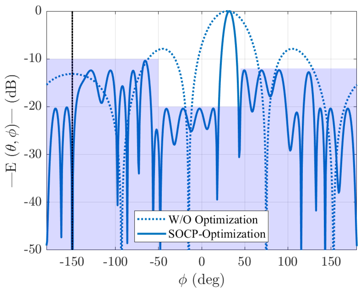
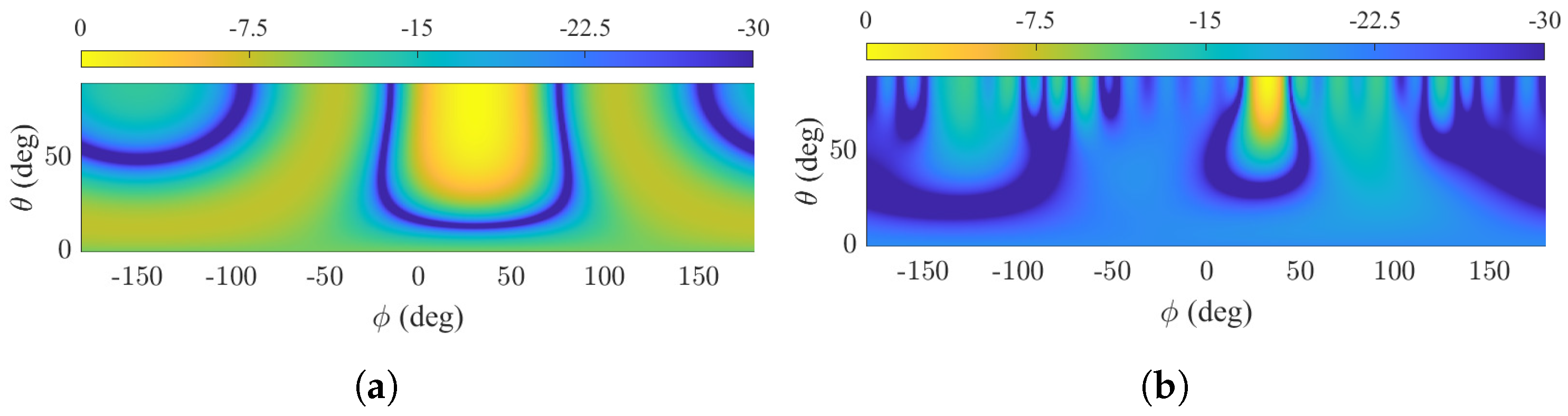
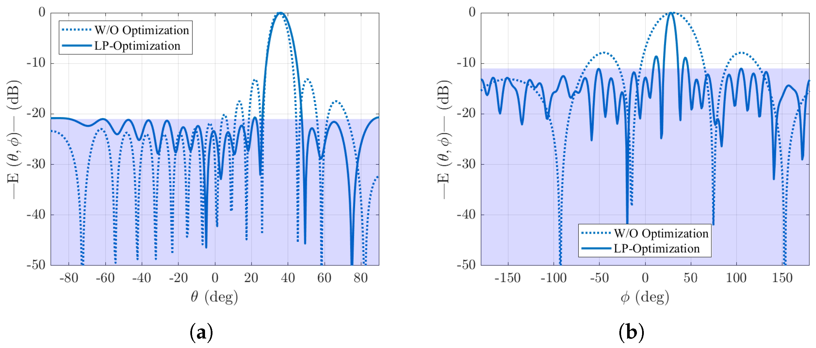
Results for Reducing SLLs Through LP

Once again, taking as a reference the geometries of the square and circular arrays used in the previous sections, they were used to perform an LP optimization. In this case, the sole objective was to reduce the SLL levels outside the main beam. Figure 9 shows the radiation pattern before and after the LP optimization for the main beam cut in both arrays. In the square array, the SLL level was reduced to below $-21\mathrm{dB}$ over the entire angular range, successfully reducing the SLLs compared to the classic excitation. This reduction in SLLs occurred over the entire visible range except for the interval that contained the main beam. In the case of the circular array, it was possible to reduce the SLLs below $-11\mathrm{dB}$ over the entire visible range $\varphi \in \left[-{180}^{\circ },{180}^{\circ }\right]$, with the first sidelobes slightly exceeding that level. Compared to the classic excitation, not only was the SLL level drastically reduced, but as a direct consequence, the main beam was also narrowed around the pointing direction $({\theta }_0,{\varphi }_0)=({90}^{\circ },{30}^{\circ })$. These results can be better evaluated in Figure 10, where the $\theta –\varphi$ plane is shown. It can be observed that the sidelobes were reduced throughout the entire plane and by eliminating radiation in undesired directions, the power was concentrated around the main beam, achieving a reduction in both $\theta$ and $\varphi$.

6. Discussion

The results obtained in this work demonstrate the significant potential of convex optimization for antenna array synthesis. By formulating the radiation pattern design problem as the maximization of directivity through a Rayleigh quotient of Hermitian forms, we developed a unified framework that leveraged quadratic programming (QP), second-order cone programming (SOCP), and linear programming (LP) to address different aspects of the optimization process.

In our QP formulation, directivity was maximized while null constraints were imposed, effectively tailoring the beam to suppress interference in specific directions. This approach not only enhanced the main beam performance but also ensured precise null placement. Building on this, the SOCP formulation extended the capabilities by incorporating additional constraints to minimize sidelobe levels (SLLs), thereby achieving a more refined control over the entire radiation pattern. In cases where the primary objective was SLL reduction, the LP formulation, which was derived as a special case of SOCP, proved to be a computationally efficient alternative.

Numerical experiments on both rectangular and circular array geometries confirmed the effectiveness of the proposed methods. The QP approach yielded higher directivity with clearly defined nulls, while the SOCP and LP formulations successfully reduced sidelobe levels. These results demonstrated that convex optimization provided not only global optimality but also significant computational advantages compared to more traditional methods.

The broader implications of this work are twofold. First, it establishes a systematic methodology for radiation pattern synthesis that is both mathematically rigorous and practically efficient. Second, it opens the door for further exploration into hybrid optimization strategies that could combine the strengths of QP, SOCP, and LP with other heuristic techniques, including convex relaxation approaches, to better handle complex constraints and uncertainties inherent in real-world array designs. Future research may also extend these techniques to larger and more adaptive array geometries, further pushing the boundaries of high-performance antenna design.

Overall, the integration of convex optimization techniques in antenna array synthesis, as presented in this work, provides valuable insights into the trade-offs between formulation complexity and pattern performance, and it underscores the potential for these methods to revolutionize modern array design.

References

1. Larsson, E.G.; Edfors, O.; Tufvesson, F.; Marzetta, T.L. Massive MIMO for next generation wireless systems. IEEE Commun. Mag. 2014, 52, 186–195. [Google Scholar] [CrossRef]
2. Liu, F.; Cui, Y.; Masouros, C.; Xu, J.; Han, T.X.; Eldar, Y.C.; Buzzi, S. Integrated sensing and communications: Toward dual-functional wireless networks for 6G and beyond. IEEE J. Sel. Areas Commun. 2022, 40, 1728–1767. [Google Scholar] [CrossRef]
3. Hasch, J.; Topak, E.; Schnabel, R.; Zwick, T.; Weigel, R.; Waldschmidt, C. Millimeter-wave technology for automotive radar sensors in the 77 GHz frequency band. IEEE Trans. Microw. Theory Techn. 2012, 60, 845–860. [Google Scholar] [CrossRef]
4. Uzkov, A.I. An approach to the problem of optimum directive antenna design. C.R. Acad. Sci. USSR 1946, 53, 35–38. [Google Scholar]
5. Bloch, R.G.M.A.; Pool, S.D. A new approach to the design of superdirective aerial arrays. Proc. Inst. Electr. Eng. 1953, 100, 303–314. [Google Scholar]
6. Uzsoky, M.; Solymar, L. Theory of superdirective linear arrays. Acta Phys. 1956, 6, 185–204. [Google Scholar] [CrossRef]
7. Lo, S.W.L.Y.T.; Lee, Q.H. Optimization of directivity and signal-to-noise ratio of an arbitrary antenna array. Proc. IEEE 1966, 54, 1033–1045. [Google Scholar] [CrossRef]
8. Krupitskii, E.I. On the maximum directivity of antennas consisting of discrete radiators. Sov. Phys. Dokl. 1962, 7, 257–259. [Google Scholar]
9. Tai, C.T. The optimum directivity of uniformly spaced broadside arrays of dipoles. IEEE Trans. Antennas Propag. 1964, 12, 447–454. [Google Scholar] [CrossRef]
10. Cheng, D.K.; Tseng, F.I. Maximisation of directive gain for circular and elliptical arrays. Proc. IEEE 1967, 114, 589–594. [Google Scholar] [CrossRef]
11. Cheng, D.K.; Tseng, F.I. Gain optimization for arbitrary antenna arrays. IEEE Trans. Antennas Propag. 1967, 13, 973–974. [Google Scholar] [CrossRef]
12. Bhattacharyya, A.K. Phased Array Antennas: Floquet Analysis, Synthesis, BFNs, and Active Array Systems; Wiley-Interscience: Hoboken, NJ, USA, 2006. [Google Scholar]
13. Cheng, D.K. Optimization techniques for antenna arrays. Proc. IEEE 1971, 59, 1664–1674. [Google Scholar] [CrossRef]
14. Einarsson, O. Optimization of planar arrays. IEEE Trans. Antennas Propag. 1979, 27, 86–92. [Google Scholar] [CrossRef]
15. Tseng, F.I.; Cheng, D.K. Optimum scannable planar arrays with an invariant sidelobe level. Proc. IEEE 1968, 56, 1771–1778. [Google Scholar] [CrossRef]
16. Ares-Pena, F.J.; Rodriguez-Gonzalez, J.A.; Villanueva-Lopez, E.; Rengarajan, S.R. Genetic algorithms in the design and optimization of antenna array patterns. IEEE Trans. Antennas Propag. 1999, 47, 506–510. [Google Scholar] [CrossRef]
17. Donelli, M.; Martini, A.; Massa, A. A hybrid approach based on PSO and Hadamard difference sets for the synthesis of square thinned arrays. IEEE Trans. Antennas Propag. 2009, 57, 2491–2495. [Google Scholar] [CrossRef]
18. Li, J.; Liu, Y.; Zhao, W.; Zhu, T. Application of Dandelion Optimization Algorithm in Pattern Synthesis of Linear Antenna Arrays. Mathematics 2024, 12, 1111. [Google Scholar] [CrossRef]
19. Bulatsyk, O.; Katsenelenbaum, B.; Topolyuk, Y.; Voitovich, N. Phase Optimization Problems: Applications in Wave Field Theory; Wiley-VCH: Weinheim, Germany, 2010. [Google Scholar]
20. Andriychuk, M. Antenna Synthesis Through the Characteristics of Desired Amplitude; Cambridge Scholars Publishing: Newcastle upon Tyne, UK, 2019. [Google Scholar]
21. Nocedal, J.; Wright, S.J. Numerical Optimization; Springer: Berlin/Heidelberg, Germany, 2000. [Google Scholar]
22. Ng, B.P.; Er, M.H.; Kot, C. A flexible array synthesis method using quadratic programming. IEEE Trans. Antennas Propag. 1993, 41, 1541–1550. [Google Scholar] [CrossRef]
23. Lebret, H.; Boyd, S. Antenna array pattern synthesis via convex optimization. IEEE Trans. Signal Process. 1997, 45, 526–532. [Google Scholar] [CrossRef]
24. Corcoles, J.; Gonzalez, M.A.; Rubio, J. Multiobjective optimization of real and coupled antenna array excitations via primal-dual, interior point filter method from spherical mode expansions. IEEE Trans. Antennas Propag. 2009, 57, 110–121. [Google Scholar] [CrossRef]
25. Holm, S.; Elgetun, B. Properties of the beampattern of weight- and layout-optimized sparse arrays. IEEE Trans. Ultrason. Ferroelectr. Freq. Control 1997, 44, 983–991. [Google Scholar] [CrossRef]
26. Corcoles, J.; Gonzalez, M.A.; Zapata, J. Linear programming from generalised scattering matrix analysis of array for minimum sidelobe level and prescribed nulls. Electron. Lett. 2009, 45, 9–10. [Google Scholar] [CrossRef]
27. Kurth, R.R. Optimization of array performance subject to multiple power constraints. IEEE Trans. Antennas Propag. 1974, 22, 103–105. [Google Scholar] [CrossRef]
28. Hirasawa, K. The application of a biquadratic programming method to phase-only optimization of antenna arrays. IEEE Trans. Antennas Propag. 1988, 36, 1545–1550. [Google Scholar] [CrossRef]
29. Lobo, M.S.; Vandenberghe, L.; Boyd, S.; Lebret, H. Applications of second-order cone programming. Linear Algebra Appl. 1998, 284, 193–228. [Google Scholar] [CrossRef]
30. Corcoles, J.; Gonzalez, M.A.; Rubio, J. Mutual coupling compensation in arrays using a spherical wave expansion of the radiated field. IEEE Antennas Wirel. Propag. Lett. 2009, 8, 108–111. [Google Scholar] [CrossRef]
31. Corcoles, J.; Zastrow, E.; Kuster, N. Convex optimization of MRI exposure for mitigation of RF-heating from active medical implants. Phys. Med. Biol. 2015, 60, 7293–7308. [Google Scholar] [CrossRef]
32. Gantmacher, F.R. The Theory of Matrices, Volume One; Chelsea Publishing Company: New York, NY, USA, 1959. [Google Scholar]
Figure 1. Scheme of a generic array antenna with a uniform distribution of the elements using a (a) rectangular and (b) circular configuration.
Mathematics 13 01796 g001
Figure 2. Radiation pattern using classic excitations (dotted line) and optimized with QP (solid line) for a (a) square array and (b) circular array. The optimization goal is to maximize directivity.
Mathematics 13 01796 g002
Figure 3. Radiation pattern using classic excitations and optimized with QP for a (a) square array and (b) circular array. The optimization goal is to maximize directivity and place nulls in the directions marked by the black vertical lines.
Mathematics 13 01796 g003
Figure 4. Excitation coefficients for the (a) square and (b) circular arrays before and after the QP-based optimization with null directions. Each color corresponds to an element.
Mathematics 13 01796 g004
Figure 5. Radiation pattern of an unoptimized square array (dotted line) and an SOCP-based optimized square array (solid line) for (a) maximizing directivity and (b) nulls. The directions for placing the nulls are marked with the dashed black lines.
Mathematics 13 01796 g005
Figure 6. (a) Radiation pattern of an unoptimized square array and a SOCP-based optimized square array for maximizing directivity, forcing nulls (black vertical lines), and reducing SLL level. (b) Samples of the excitation vector a obtained after and before the SOCP-based optimization. Each color corresponds to an element.
Mathematics 13 01796 g006
Figure 7. Radiation pattern before and after the SOCP-based optimization imposing SLL requirements and two null in the directions marked by the black vertical lines.
Mathematics 13 01796 g007
Figure 8. Radiation pattern in the θ ϕ plane using (a) the classic excitation and (b) the SOCP-optimized excitation. Each color corresponds to an element.
Mathematics 13 01796 g008
Figure 9. (a) Radiation pattern of an unoptimized square array and a LP-based optimized square array for reducing SLL level (b) circular array and a LP-based optimized circular array for reducing SLL level.
Mathematics 13 01796 g009
Figure 10. Radiation pattern of the circular array (a) before and (b) after the LP-based optimization to reduce the SLL level.
Mathematics 13 01796 g010
Disclaimer/Publisher’s Note: The statements, opinions and data contained in all publications are solely those of the individual author(s) and contributor(s) and not of MDPI and/or the editor(s). MDPI and/or the editor(s) disclaim responsibility for any injury to people or property resulting from any ideas, methods, instructions or products referred to in the content.