State Estimation Based State Augmentation and Fractional Order Proportional Integral Unknown Input Observers

Abstract

This paper presents a new method for the simultaneous estimation of system states and unknown inputs in fractional-order Takagi–Sugeno (FO-TS) systems with unmeasurable premise variables (UPVs), by introducing a fractional-order proportional-integral unknown input observer (FO-PIUIO) based on partial state augmentation. This approach permits the estimation of both states and unknown inputs, which are essential for system monitoring and control. Partial state augmentation allows the integration of unknown inputs into a partially augmented model, ensuring accurate estimates of both states and unknown inputs. The state estimation error is formulated as a perturbed system. The convergence conditions for the state estimation errors between the system and the observer are derived using the second Lyapunov method and the $L_2$ approach. Compared to traditional integer-order unknown input observers or fuzzy observers with measurable premise variables, in our method, fractional-order dynamics are combined with partial state augmentation uniquely for the persistent estimation of states along with unknown inputs in unmeasurable premise variable systems. Such a combination allows for robust estimation even under uncertainties in systems and long memory phenomena and is a significant step forward from traditional methods. Finally, a numerical example is provided to illustrate the performance of the proposed observer.

1. Introduction

State estimation plays a fundamental role in the control and monitoring of dynamic systems, with specific reference to nonlinear behaviors and disturbances. Classical linear models are not always able to properly describe the complexity of actual systems, and for this reason, more sophisticated approaches, e.g., Takagi–Sugeno (T-S) fuzzy models, have been exploited. They are able to model nonlinear systems through interpolating a set of linear sub-models via fuzzy membership functions, thus making it possible to apply linear system analysis techniques to nonlinear cases [1]. Owing to their versatility and effectiveness, the models have found extensive applications in many fields, including control system design, fault diagnosis, and intelligent systems [2].

In spite of their benefits, state estimation in such models is still a daunting task, particularly in the presence of unmeasured disturbances and unobservable premise variables (UPVs). This is especially true in fields of application such as robotics, power systems, and biomedical engineering, where system uncertainties and measurement imprecisions can greatly affect performance [3]. One of the primary approaches to tackle this difficulty is the development of robust observers specifically for fuzzy systems. Chadli and Karimi [4] proposed a robust unknown input observer for Takagi–Sugeno models, providing LMI-based conditions to ensure stable estimation despite unknown disturbances affecting states and outputs.

In a related work, ref. [5] investigated the design of finite-time bounded tracking controllers designed for fractional-order systems subject to state delays using output feedback for reducing the effects of temporal delays and the dynamics of the systems. However, their method revolves more around control design rather than our proposed algorithm, the FO-PIUIO, where the estimation of both the state and unmeasured inputs is given the first priority. As opposed to the method that Wu et al. utilized where the problem of UPVs was not directly addressed, the FO-PIUIO is specifically designed to handle this problem in the context of fractional-order dynamics as well as UPVs. Combining fractional-order dynamics and robust estimation methods gives the FO-PIUIO a more integrated solution for state estimation and disturbance elimination.

The FO-PIUIO introduced here successfully addresses a key theoretical gap by extending the application of integer-order UIOs and fuzzy observers to fractional-order dynamic systems. In comparison with integer-order approaches that routinely struggle with the treatment of memory effects and long-term dependences of dynamic systems, our proposed fractional-order method incorporates such intricacies for a higher level of accuracy and robustness of state and unknown input estimations.

Existing literature, such as the nonlinear unknown input observer (NUIO) cited by [6], has provided effective fault-tolerant methods for integer-order electro-hydraulic systems. However, this method assumes fully measurable nonlinearities and does not account for fractional-order dynamics as well as hidden state-dependent interactions. Such limitations make it less applicable to those systems that display memory effects and hereditary traits or unobservable premise variables—phenomena common in modern industrial and biological applications.

The unknown input observer (UIO) design principles were established by using system redundancy along with filtering concepts, enhancing state estimation in nonlinear control systems [7]. These observers have found extensive application in fields such as industrial automation, safety-critical systems, and fault-tolerant control, where robustness to model uncertainty is of the utmost importance.

One of the most significant features of the Takagi–Sugeno fuzzy modeling framework is that it is based on premise variables that dictate the firing of fuzzy rules. Two types of premise variables exist: measurable premise variables (MPVs) and unmeasurable premise variables (UPVs). MPVs are premise variables that are directly measurable or calculable from the outputs of the system. MPV-based FO-TS systems have observers that are able to utilize the data available to enhance the precision of state estimation. UPVs, however, utilize internal system states, which are not readily measurable, and observer design becomes challenging with the need for further estimation methods to reconstruct both the system state and premise variables.

The MPV-UPV distinction is critical in observer design for state estimation. MPV systems allow for the systematic design of observers with the benefit of known premise dynamics. In UPV systems, however, state estimation entails the necessity for additional augmentation strategies to treat uncertainties. The state augmentation approach formulated in this paper presents a unified framework to treat MPV and UPV cases with unknown inputs and disturbances robustness.

One of the noteworthy advancements in the field of T-S modeling is the application of fractional-order dynamics, which enable the inclusion of memory and hereditary influences by using fractional derivatives [8]. It has enhanced the modeling precision of dynamic systems in various fields, such as electromechanical systems, bioengineering, and industrial processes [9]. Fractional-order fuzzy models are more capable of describing real-world behaviors than integer-order models, especially for systems with long-range dependencies [10]. But state estimation in these models is more complex, especially in the case of unmeasurable premise variables, where it is required to design sophisticated observers that are able to reconstruct system states and unknown inputs.

Unlike traditional integer-order UIO designs, the FO-PIUIO benefits from the utilization of fractional-order dynamics within the system to enable improved modelling of long-range-dependent systems. In addition, as opposed to fuzzy observer methods that traditionally assume the availability of measurable premise variables (MPVs), our method can perform under the conditions of unmeasurable premise variables (UPVs). With this ability comes the capacity for precise state and unknown input estimations under more complex and uncertain conditions. Therefore, the FO-PIUIO becomes particularly beneficial under conditions involving uncertainties and disturbances.

A significant advancement in this area has been the establishment of fractional-order unknown input observers for application in nonlinear systems based on fractional-order fuzzy models that are subject to unmeasurable premise variables (UPVs) [11]. These observers allow for robust state estimation and fault detection without the need to alter the original model of the system, thereby rendering them extremely desirable for practical implementation. Stability and convergence analyses of these observers are generally carried out by Lyapunov-based approaches, in which the conditions are expressed in terms of linear matrix inequalities to facilitate easy implementation of robust observer and controller designs [12]. The use of optimization methods based on linear matrix inequalities is common in control theory due to their ability to guarantee reliable performance under system uncertainties and external disturbances [13]. The performance of fractional-order unknown input observers has been validated in a wide range of applications, ranging from robotics to power electronics, and fault detection systems [14].

Recent advances have also explored further the application of machine learning-based approaches in state estimation accuracy improvement. The construction of a hybrid observer through the combination of data-driven approaches and classical observer designs has been reported to improve adaptive estimation in varying conditions and improve real-time performance [15]. In parallel, advances in observer-based fault diagnosis have also been prominent, particularly in sensor fault detection and isolation. Observer-based fault detection methods using structured residuals have been designed with the aim of sensor fault detection and isolation with enhanced robustness compared to the standard fault detection methods, rendering them apt for application in real-time industrial environments [16].

Other developments in fault diagnosis include the development of sensor fault detection techniques based on multiple observer schemes, which are designed with a view to nullify unknown inputs while maintaining the integrity of fault isolation [17]. Such multiple observer systems have been widely used in safety-critical applications like aerospace systems and industrial process control, where accurate fault isolation is crucial in maintaining operational integrity. Model-based fault diagnosis methods have been emphasized as the most important strategy for enhancing the reliability of systems operating under stochastic environments [18]. The application of fractional-order dynamics in observers for fault diagnosis has achieved an immense advancement and thus reemphasized the relevance of high-order observer technologies in contemporary control systems [19].

A recent paper has illustrated a fractional-order fuzzy observer designed for a fuzzy model with immeasurable premise variables, enhancing the accuracy of estimation in systems subject to severe uncertainty. The paper presents a novel observer structure, proving its efficiency in fault detection scenarios and enhancing the robustness of fractional-order observer methods [20]. Beyond these advances, ongoing work on the unspecified input observers of nonlinear systems has investigated their capability to achieve more precise state estimation and unknown inputs. Such questions continue to introduce resilience and enhance the usefulness of observer design in sophisticated control systems [21].

While existing methods of unknown input observers (UIOs) and fuzzy observer designs for fractional-order systems primarily deal with measurable premise variables (MPVs), the field of research on observers of fractional-order Takagi–Sugeno (FO-TS) systems with respect to unmeasurable premise variables (UPVs) is less explored. Further, existing methods do not provide a complete coverage of state augmentation for better state and unknown input estimation in these systems. This paper attempts to fill this gap by designing a new fractional-order proportional-integral unknown input observer (FO-PIUIO) for FO-TS systems with UPVs via partial state augmentation for improved estimation quality and robustness against unmeasurable premise variables and unknown inputs.

This paper proposes a novel fractional-order proportional-integral unknown input observer (FO-PIUIO) design for fractional-order Takagi–Sugeno systems with MPVs and UPVs to enhance the estimation accuracy and robustness of the state and to address the problems raised by unmeasurable premise variables and unknown inputs. Among the contributions of this paper is the importance of state augmentation, which is an inherent component of improved estimation quality. By adding the unknown inputs to the system model, state augmentation allows for a closer approximation of the system dynamics free from estimation bias and, therefore, ensures consistent observer behavior.

The approach to be suggested employs linear matrix inequalities (LMIs) in the design of stability conditions and the optimization of observer gains to ensure the asymptotic convergence of state estimation errors. The main contributions of this paper include the development of a novel fractional-order unknown input observer through state augmentation for more precise estimation; stability condition derivation through Lyapunov-based analysis and LMI optimization for the asymptotic convergence of the estimation errors; the generalization of this method to MPV-based and UPV-based FO-TS models, which solves an open problem in observer-based control; and comprehensive numerical verification, which demonstrates the potential of the proposed observer in handling unknown inputs, removing estimation bias, and improving robustness in dynamic systems.

The organization of the rest of this paper is as follows. First, the problem statement and system model are presented, followed by the suggested observer design and stability condition derivation. Numerical simulations are provided to validate the effectiveness of the suggested method. The conclusion and potential future research directions are presented in the last section.

2. Comprehensive Theoretical Basis

2.1. Fractional Calculus: Definitions and Notation

In this work, the operator ${}_{t_0}D_t^{\alpha }$ denotes the Caputo fractional derivative of order $\alpha >0$, which is defined for a sufficiently smooth function $x\left(t\right)$ as follows [8,11]:

$${}_{t_0}D_t^{\alpha }x\left(t\right)={\displaystyle \frac{1}{\mathrm{\Gamma }\left(n-\alpha \right)}}{\displaystyle {\int }_0^t\frac{x^{\left(n\right)}\left(\tau \right)}{{\left(t-\tau \right)}^{\alpha -n+1}}d\tau ,}$$

where $n=\left[\alpha \right]$ is the smallest integer greater than or equal to $\alpha$, $\alpha >0$, and $\mathrm{\Gamma }\left(\hspace{0.17em}.\hspace{0.17em}\right)$ is the Gamma function.

$\mathrm{\Gamma }\left(z\right)$ generalizes the factorial to real and complex numbers and is given by the following [8,11]:

$$\mathrm{\Gamma }\left(z\right)={\displaystyle {\int }_0^{\infty }{t}^{z-1}{e}^{-t}dt,} \mathrm{for} z>0.$$

These definitions are central in modeling systems with memory and hereditary dynamics, which are intrinsic to fractional-order models.

2.2. Principle of State Augmentation and FO-PIUIO Design

A system often undergoes concurrent influence by separate inputs that represent its control signals, in addition to inputs that cannot be easily identified, which can include disturbances, measurement noise, modeling errors, or faults. As such, the design of a state observer that ignores these unidentifiable inputs can lead to degraded or even erroneous state estimates. In such cases, developing control laws or residual generators for fault detection, based on these estimated states, leads to suboptimal system performance [17].

To counteract the estimation bias inherent in state estimators without incurring additional modeling efforts, there is a need to design observers that can provide accurate state estimations regardless of any unknown inputs. This requirement calls for the inclusion of such unknown inputs in the modeling framework.

Indeed, including all possible variables that may affect the system—e.g., measurement noise, faults, and modeling uncertainties—within the system model helps enhance the estimation quality.

The pre-specified framework, termed the reference model, in conjunction with the input and output measurements extracted from the actual system, is utilized to facilitate the selection of a suitable augmented model. This process begins with an initial model, recognized as the reference model, which is expressed in a fractional-order state-space representation:

$$\left\{\begin{array}{l}{}_{t_0}D_t^{\alpha }x=f(x,u)\hfill \\ y=h(x)\hfill \end{array}\right.$$

(1)

where $x$ is the state vector, $u$ is the known control inputs, and $y$ is the measurement vector. The parameter $\alpha$ is the fractional order with some conditions, and $f$ and $h$ are nonlinear functions. The goal is to develop a systematic process for designing a fractional-order observer that will give an unbiased estimate of the system state. This must be done even if the reference model is contaminated with unknown inputs.

An easy way to achieve an unbiased state estimation even for the unknown input case $q(t)$ is to extend the reference model by these unknown inputs as follows:

$$\left\{\begin{array}{c}{}_{t_0}D_t^{\alpha }x=\hat{f}(x,u,q)\\ y=\hat{h}(x,q)\end{array}\right.$$

(2)

and the design of the fractional-order observer using this augmented fractional-order model. If the augmentation effectively captures the unknown inputs and the augmented fractional-order system remains observable, the state estimations will be unbiased.

An obvious question then arises: how should the unknown inputs $q(t)$ be introduced into the fractional-order model equations? One possible approach is through prior knowledge of the underlying processes.

In practice, the above knowledge could be the structural knowledge in the shape of disturbances affecting the system, noise behavior modeling, or hypothesized fault signal dynamics. The assumptions are used to inform the upgraded model structure so that it is observable and suitable for effective use by the envisaged FO-PIUIO. The formalization of the procedure is addressed in the next section in the shape of the mathematical development of the partially augmented FO-TS system and associated observer structure.

3. Method

3.1. Partial Augmentation of the FO-TS System with VDM and FO-PIUIO Design

State and unknown input estimation based on the system’s input–output data can be addressed for linear systems using the proportional-integral unknown input observer (FO-PIUIO). Due to the inefficiency of proportional observers in the presence of unknown inputs acting on the system, the PI observer has been proposed as a solution for estimating unknown inputs.

In this section, the study of the FO-PIUIO will be developed for both the cases of measurable premise variables (MPVs) and unmeasurable premise variables (UPVs). Here, the unknown inputs are assumed to be constant.

3.1.1. Partial Augmentation of FO-TS with MPVs

In this section, we outline the process of partial state augmentation for the MPV-affected FO-TS system. The primary objective is to demonstrate how state augmentation can incorporate the unknown inputs in the system model without influencing the system observability. By introducing the system with measurable premise variables, we expect to improve the observer’s ability in estimating the state and the unknown inputs of the system. The approach ensures that the observer is precise and stable regardless of the existence of unknown disturbances.

Consider the fractional-order Takagi–Sugeno (FO-TS) system with measurable decision variables, where the influence matrices of the unknown inputs differ:

$$\left\{\begin{array}{l}{}_{t_0}D_t^{\alpha }x(t)={\displaystyle \sum _{i=1}^M{h}_i(x(t))\left(A_{i}x(t)+B_{i}u(t)+E_i{q}_1(t)\right)}\hfill \\ y(t)=Cx(t)+E{q}_2(t)\hfill \end{array}\right.$$

(3)

In this formulation, $h_i\left(x\left(t\right)\right)$ are the normalized activation functions (or membership functions) of the Takagi–Sugeno fuzzy model, satisfying ${\displaystyle \sum _{i=1}^M{h}_i\left(x\left(t\right)\right)=1}$ and $h_i\left(x\left(t\right)\right)\ge 0$. The matrices $A_i\in R^{n\times n}$ represent the local state matrices, $B_i\in R^{n\times n_u}$ are the local input matrices associated with the known inputs $u\left(t\right)$, $E_i\in R^{n\times n_{q_1}}$ is the influence matrix corresponding to the unknown inputs $q_1\left(t\right)$, and $E\in R^{n\times n_q}$ is the influence matrix corresponding to the second group of unknown inputs $q_2\left(t\right)$. The parameter $M$ denotes the number of local linear sub-models used in the Takagi–Sugeno fuzzy system, which is determined by the fuzzy rule base and does not change during the state augmentation process.

The system can be rewritten in the following form:

$$\left\{\begin{array}{l}{}_{t_0}D_t^{\alpha }x(t)={\displaystyle \sum _{i=1}^M{h}_i(x(t))\left(A_{i}x(t)+B_{i}u(t)+E_i{q}_1(t)\right)}\hfill \\ y(t)=\left[{\displaystyle \frac{C^{p,1}}{C^{p,2}}}\right]x(t)+\left[{\displaystyle \frac{0}{E^{q,1}}}\right]q_2(t)\hfill \end{array}\right.$$

(4)

where $C^{p,1}\in R^{(p-q)\times n}$ and $C^{p,2}\in R^{q\times n}$.

By utilizing the property ${\displaystyle \sum _{i=1}^M{h}_i\left(x\left(t\right)\right)=1}$ and $h_i\left(x\left(t\right)\right)\ge 0$, the state $g_f(t)$ can be rewritten as follows:

$$g_f(t)={\displaystyle \sum _{i=1}^M{h}_i(x(t))\left[-A_{f_i}{g}_f(t)+A_{f}Cx(t)+A_{f}Eu(t)\hspace{0.17em}\right]}$$

where $A_f\in R^{p\times p}$ is a stable matrix.

The augmented system is given as follows:

$$\left\{\begin{array}{l}{}_{t_0}D_t^{\alpha }{x}_a(t)={\displaystyle \sum _{i=1}^M{h}_i(x(t))\left[A_{ai}{x}_a(t)+B_{ai}u(t)+E_{ai}q(t)\hspace{0.17em}\right]}\hfill \\ y(t)=C_a{x}_a(t)\hfill \end{array}\right.$$

(5)

with

$$x_a(t)=\left[\begin{array}{c}x(t)\\ g_f(t)\end{array}\right], q(t)=\left[\begin{array}{c}{q}_1(t)\\ q_2(t)\end{array}\right], A_{ai}=\left[\begin{array}{cc}{A}_i& 0\\ A_{fi}{C}^{p,2}& -A_{fi}\end{array}\right],$$

$$B_{ai}=\left[\begin{array}{c}{B}_i\\ 0\end{array}\right], C_a=\left[\begin{array}{cc}{C}^{p,1}& 0\end{array}\right], E_{ai}=\left[\begin{array}{cc}{E}_i& 0\\ 0& A_{fi}{E}^{q,1}\end{array}\right]$$

The augmentation procedure demonstrated in this part shows how to efficiently tackle systems with measurable premise variables. This allows the synthesis of an efficient observer for estimating states and unknown inputs. What follows will be an extension of this by taking into account the situation of unmeasurable premise variables (UPVs), which introduces complexities to the observer synthesis.

3.1.2. FO-PIUIO Design of Augmented FO-TS System with MPVs

The proposed fractional-order proportional-integral unknown input observer is given in the following form:

$$\left\{\begin{array}{l}{}_{t_0}D_t^{\alpha }z(t)={\displaystyle \sum _{i=1}^M{h}_i(x(t))\left[N_{i}z(t)+G_{i}u(t)+F_i\hat{q}(t)+L_i^{P}y(t)\right]}\hfill \\ {\hat{x}}_a(t)=z(t)+Hy(t)\hfill \\ {}_{t_0}D_t^{\alpha }\tilde{q}(t)=-{\displaystyle \sum _{i=1}^M{h}_i(x(t))L_i^I\left[y(t)-\hat{y}(t)\right]}\hfill \\ \hat{y}(t)=C_a{\hat{x}}_a(t)\hfill \end{array}\right.$$

(6)

$N_i(t)\in R^{n\times n}$ and $G_i(t)\in R^{n\times m}$ are the fractional-order proportional-integral unknown input observer, $L_i(t)\in R^{n\times p}$ is the gain of the ith local observer, and $H$ is a transformation matrix. $L_i^P$ represents the proportional gains, and $L_i^I$ represents the integral gains of the observer (6). $\tilde{q}(t)$ represents the estimation error of the unknown input, defined by $\tilde{q}(t)=q(t)-\hat{q}(t)$.

The state estimation error is defined by the following equation:

$$\begin{array}{l}e(t)=x_a(t)-{\hat{x}}_a(t)\\ \hspace{1em}\hspace{0.33em}\hspace{0.33em}\hspace{0.17em}=(I-H{C}_a)x_a(t)-z(t)\end{array}$$

(7)

Its time derivative is expressed as follows:

$${}_{t_0}D_t^{\alpha }e(t)={\displaystyle \sum _{i=1}^M{h}_i(x(t))(P(A_{ai}{x}_a(t)+B_{ai}u(t)+E_{ai}q(t))-N_{i}z(t)-G_{i}u(t)-F_i\hat{q}(t)-L_i^{P}y(t))}$$

(8)

with

$$P=I-H{C}_a$$

(9)

Expression (8) can also be rewritten as follows:

$${}_{t_0}D_t^{\alpha }e(t)={\displaystyle \sum _{i=1}^M{h}_i(x(t))(N_{i}e(t)+(P{A}_{ai}-N_i-K_i{C}_a)x(t)+(P{B}_{ai}-G_i)u(t)+(P{E}_{ai}-F_i)q(t)+F_i\tilde{q}(t))}$$

(10)

with $K_i=L_i^P-N_{i}H$.

If the following conditions are imposed:

$$P=I-H{C}_a$$

(11)

$$N_i=P{A}_{ai}-K_i{C}_a$$

(12)

$$L_i^P=K_i+N_{i}H$$

(13)

$$G_i=P{B}_{ai}$$

(14)

$$F_i=P{E}_{ai}$$

(15)

The state reconstruction error asymptotically tends to zero, and (10) reduces to the following:

$${}_{t_0}D_t^{\alpha }e(t)={\displaystyle \sum _{i=1}^M{h}_i(x(t))\left(N_{i}e(t)+F_i\tilde{q}(t)\right)}$$

(16)

The equation governing the dynamics of the unknown input estimation error is given by the following:

$${}_{t_0}D_t^{\alpha }\tilde{q}(t)={}_{t_0}D_t^{\alpha }q(t)-{}_{t_0}D_t^{\alpha }\hat{q}(t)=-{\displaystyle \sum _{i=1}^M{h}_i(x(t))L_i^I{C}_{a}e(t)}$$

(17)

The augmented system of the state estimation error dynamics and the unknown input can be written as follows:

$${}_{t_0}D_t^{\alpha }{e}_a(t)={\displaystyle \sum _{i=1}^M{h}_i(x(t))\left[\begin{array}{cc}{N}_i& F_i\\ -L_i^I{C}_a& 0\end{array}\right]e_a(t)}$$

(18)

where $e_a(t)=\left[\begin{array}{c}e(t)\\ \tilde{q}(t)\end{array}\right]$.

Using (12), Equation (18) can be rewritten as follows:

$${}_{t_0}D_t^{\alpha }{e}_a(t)={\displaystyle \sum _{i=1}^M{h}_i(x(t))\left({\overline{A}}_i-{\overline{K}}_i\overline{C}\right)e_a(t)}$$

(19)

with

$${\overline{A}}_i=\left[\begin{array}{cc}P{A}_{ai}& F_i\\ 0& 0\end{array}\right],\hspace{1em}{\overline{K}}_i=\left[\begin{array}{c}{K}_i\\ L_i^I\end{array}\right]\hspace{1em}\mathrm{et} \hspace{1em}{\overline{C}}_a=\left[\begin{array}{cc}{C}_a& 0\end{array}\right]$$

(20)

The convergence conditions for the state and unknown input estimation errors are obtained using the following quadratic Lyapunov function:

$$V\left(e(t)\right)=e_a{(t)}^{T}X{e}_a(t),\hspace{1em}X=X^T>0$$

(21)

Its derivative is given by the following:

$${}_{t_0}D_t^{\alpha }V\left(e(t)\right)={}_{t_0}D_t^{\alpha }{e}_a{(t)}^{T}X{e}_a(t)+e_a{(t)}^{T}X{}_{t_0}D_t^{\alpha }{e}_a(t)$$

(22)

Using relation (20), it becomes as follows:

$${}_{t_0}D_t^{\alpha }V\left(e(t)\right)={\displaystyle \sum _{i=1}^M{h}_i(x(t))\left(e_a{(t)}^T({\overline{A}}_i^{T}X+X{\overline{A}}_i-{\overline{C}}^T{\overline{K}}_i^{T}X-X{\overline{K}}_i\overline{C}\right)e_a(t)}$$

(23)

The derivative of the Lyapunov function is negative if the following:

$${\overline{A}}_i^{T}X+X{\overline{A}}_i-{\overline{C}}^T{\overline{K}}_i^{T}X-X{\overline{K}}_i\overline{C}<0,\hspace{1em}\forall i\in \left\{1,\dots ,M\right\}$$

(24)

To formulate an LMI-based problem, we introduce the following variable change:

$$W_i=X{\overline{K}}_i$$

(25)

Using the variable change (25), inequality (24) becomes the following:

$${\overline{A}}_i^{T}X+X{\overline{A}}_i-{\overline{C}}^T{W}_i^T-W_i\overline{C}<0$$

(26)

The gains of the FO-PIUIO are then derived using the following equation:

$${\overline{K}}_i=X^{-1}{W}_i$$

(27)

The following theorem is derived based on the conditions presented in Equation (26), which were obtained from the Lyapunov method and linear matrix inequality (LMI) analysis in the previous section. This theorem expresses the asymptotic convergence of the state and unknown input estimation errors, which is the key result of the preceding derivations:

Theorem 1.

The state estimation error and the unknown input estimation error between the fractional-order unknown input observer (6) and the fractional-order Takagi–Sugeno system with VDM (3) asymptotically converge to zero if there exists a symmetric and positive definite matrix $X$, along with matrices $W_i$ such that for $i\in \left\{1,\dots ,M\right\}:$

$${\overline{A}}_i^{T}X+X{\overline{A}}_i-{\overline{C}}^T{W}_i^T-W_i\overline{C}<0,\hspace{1em}i=1,\dots ,M$$

(28)

The gains of the FO-PIUIO are then derived using the following equation:

$${\overline{K}}_i=X^{-1}{W}_i$$

(29)

To improve the performance of the FO-PIUIO (6), its dynamics are chosen to be significantly faster than those of the FO-TS system (3).

The resolution of constraints (11)–(13) is carried out in three steps, as previously mentioned:

1.

From relation (11), the matrix $H$ is computed as follows:

$$\left[\begin{array}{cc}P& H\end{array}\right]={\left[\begin{array}{c}{I}_p\\ C_a\end{array}\right]}^T{\left(\left[\begin{array}{c}{I}_p\\ C_a\end{array}\right]{\left[\begin{array}{c}{I}_p\\ C_a\end{array}\right]}^T\right)}^{-1}$$

(30)

where $I_p$ is a full-rank identity matrix.

After solving inequality (28), the gains are determined using the following equation:

$${\overline{K}}_i=X^{-1}{W}_i$$

(31)

From Equations (12) and (13), we can compute the following:

$$G_i=P{B}_{ai}$$

(32)

$$F_i=P{E}_{ai}$$

(33)

$$N_i=P{A}_{ai}-K_i{C}_a$$

(34)

$$L_i^P=K_i+N_{i}H$$

(35)

The next subchapter deals with the UPV scenario, where all premise variables are not measurable. This brings more complexities in the design of an observer, which requires states and disturbance inputs to be closely looked at, and this affects error dynamics and stability conditions. The next section reviews approaches toward the resolution of issues arising due to the UPV scenario.

3.2. Partial Augmentation of the FO-TS System with UPV and State Estimation

In comparison, the case with unmeasurable premise variables is more complex as compared to that with measurable premise variables. A more complex observer structure is necessitated by unmeasurable premise variables to estimate the state accurately as well as unknown inputs in real time. The following summarizes the modifications introduced to the observer structure, error dynamics, and stability conditions toward the effective treatment of UPVs.

Table 1. Comparison of observer structure, error dynamics, and stability criteria between MPV and UPV Cases.

Aspect	MPV Case	UPV Case
Observer Structure	Based on measurable premise variables (MPVs)	Requires augmentation due to unmeasurable premise variables (UPVs)
Error Dynamics	Standard error dynamics for measurable variables	Error dynamics must account for unmeasurable premise variables and disturbances
Stability Criteria	Lyapunov-based stability for measurable data	Lyapunov-based stability with additional conditions to handle UPVs and unknown inputs

summarizes the key differences between MPV and UPV systems and enhances the clarity of how the observer design changes for each scenario.

3.2.1. Partial Augmentation of FO-TS with UPVs

We now consider the case where the system’s activation functions depend on non-measurable variables (e.g., the system state). The system structure is written as follows:

$$\left\{\begin{array}{l}{}_{t_0}D_t^{\alpha }{x}_a(t)={\displaystyle \sum _{i=1}^M{h}_i(x(t))\left[A_{ai}{x}_a(t)+B_{ai}u(t)+E_{ai}q(t)\hspace{0.17em}\right]}\hfill \\ y(t)=C_a{x}_a(t)\hfill \end{array}\right.$$

(36)

The equivalent form of system (36), represented by the FO-TS system with UPVs, where the activation functions depend on the estimated state, is given by the following:

$$\left\{\begin{array}{l}{}_{t_0}D_t^{\alpha }{x}_a(t)={\displaystyle \sum _{i=1}^r{h}_i(\hat{x}(t))\left(A_{ai}{x}_a(t)+B_{ai}u(t)+E_{ai}q(t)+\omega (t)\right)}\hfill \\ y(t)=C_a{x}_a(t)\hfill \end{array}\right.$$

(37)

3.2.2. State Estimation of Augmented FO-TS System with UPV

The proposed FO-PIO unknown input observer is given in the following form:

$$\left\{\begin{array}{l}{}_{t_0}D_t^{\alpha }z(t)={\displaystyle \sum _{i=1}^M{h}_i(\hat{x}(t))\left[N_{i}z(t)+G_{i}u(t)+F_i\hat{q}(t)+L_i^{P}y(t)\right]}\hfill \\ {\hat{x}}_a(t)=z(t)+Hy(t)\hfill \\ {}_{t_0}D_t^{\alpha }\tilde{q}(t)=-{\displaystyle \sum _{i=1}^M{h}_i(\hat{x}(t))L_i^I\left[y(t)-\hat{y}(t)\right]}\hfill \\ \hat{y}(t)=C_a{\hat{x}}_a(t)\hfill \end{array}\right.$$

(38)

$N_i(t)\in R^{n\times n}$ and $G_i(t)\in R^{n\times m}$ are FO-PIO unknown input observer matrices, $L_i(t)\in R^{n\times p}$ is the gain of the ith local fractional-order observer, and $H$ is a transformation matrix. $L_i^P$ represents the proportional gains, and $L_i^I$ represents the integral gains of the observer (38). $\tilde{q}(t)$ represents the estimation error of the unknown input, defined by $\tilde{q}(t)=q(t)-\hat{q}(t)$.

The state estimation error is defined by the following equation:

$$\begin{array}{l}e(t)=x_a(t)-{\hat{x}}_a(t)\\ \hspace{1em}\hspace{0.33em}\hspace{0.33em}=(I-H{C}_a)x_a(t)-z(t)\end{array}$$

(39)

Its time derivative is expressed as follows:

$${}_{t_0}D_t^{\alpha }e(t)={\displaystyle \sum _{i=1}^M\begin{array}{l}{h}_i(\hat{x}(t))(P(A_{ai}{x}_a(t)+B_{ai}u(t)+E_{ai}q(t)+\omega (t))-\\ \hspace{1em}\hspace{1em}\hspace{1em}\hspace{1em}{N}_{i}z(t)-G_{i}u(t)-F_i\hat{q}(t)-L_i^{P}y(t))\end{array}}$$

(40)

where

$$P=I-H{C}_a$$

(41)

Expression (40) can also be rewritten as follows:

$${}_{t_0}D_t^{\alpha }e(t)={\displaystyle \sum _{i=1}^M\begin{array}{l}{h}_i(\hat{x}(t))(N_{i}e(t)+(P{A}_{ai}-N_i-K_i{C}_a)x(t)+\\ \hspace{1em}\hspace{1em}\hspace{1em}\hspace{1em}(P{B}_{ai}-G_i)u(t)+(P{E}_{ai}-F_i)q(t)+F_i\tilde{q}(t)+P\omega (t))\end{array}}$$

(42)

with $K_i=L_i^P-N_{i}H$.

If the following conditions are imposed:

$$P=I-H{C}_a$$

(43)

$$N_i=P{A}_{ai}-K_i{C}_a$$

(44)

$$L_i^P=K_i+N_{i}H$$

(45)

$$G_i=P{B}_{ai}$$

(46)

$$F_i=P{E}_{ai}$$

(47)

The state reconstruction error asymptotically tends to zero, and (42) reduces to the following:

$${}_{t_0}D_t^{\alpha }e(t)={\displaystyle \sum _{i=1}^M{h}_i(\hat{x}(t))\left(N_{i}e(t)+F_i\tilde{q}(t)+P\omega (t)\right)}$$

(48)

The equation governing the dynamics of the unknown input estimation error is given by the following:

$${}_{t_0}D_t^{\alpha }\tilde{q}(t)={}_{t_0}D_t^{\alpha }q(t){}_{t_0}D_t^{\alpha }\hat{q}(t)=-{\displaystyle \sum _{i=1}^M{h}_i(\hat{x}(t))L_i^I{C}_{a}e(t)}$$

(49)

The augmented system of the fractional-order state estimation error dynamics and the unknown input can be written as follows:

$${}_{t_0}D_t^{\alpha }{e}_a(t)={\displaystyle \sum _{i=1}^M{h}_i(\hat{x}(t))\left(\left[\begin{array}{cc}{N}_i& F_i\\ -L_i^I{C}_a& 0\end{array}\right]e_a(t)+\left[\begin{array}{c}P\\ 0\end{array}\right]\omega (t)\right)}$$

(50)

where $e_a(t)=\left[\begin{array}{c}e(t)\\ \tilde{q}(t)\end{array}\right]$.

Using (44), Equation (50) can be rewritten as follows:

$${}_{t_0}D_t^{\alpha }{e}_a(t)={\displaystyle \sum _{i=1}^M{h}_i(\hat{x}(t))\left(\left({\overline{A}}_i-{\overline{K}}_i\overline{C}\right)e_a(t)+\overline{P}\omega (t)\right)}$$

(51)

with

$${\overline{A}}_i=\left[\begin{array}{cc}P{A}_{ai}& F_i\\ 0& 0\end{array}\right], {\overline{K}}_i=\left[\begin{array}{c}{K}_i\\ L_i^I\end{array}\right], {\overline{C}}_a=\left[\begin{array}{cc}{C}_a& 0\end{array}\right]\mathrm{et} \overline{P}=\left[\begin{array}{c}P\\ 0\end{array}\right]$$

(52)

By substituting $\omega (t)$ with its value,

$${}_{t_0}D_t^{\alpha }{e}_a(t)={\displaystyle \sum _{i=1}^M{h}_i(\hat{x}(t))\left(\left({\overline{A}}_i-{\overline{K}}_i\overline{C}\right)e_a(t)+\overline{P}\omega (t)\right)}$$

(53)

then $\omega (t)$ can be written in the following form:

$$\omega (t)={\displaystyle \sum _{i=1}^M\left(h_i\left(x(t)\right)-h_i\left(\hat{x}(t)\right)\right)}\left(A_{ai}{x}_a(t)+B_{ai}u(t)+E_{ai}q(t)\right)$$

(54)

$$=\mathsf{\Delta }A(t)x_a(t)+\mathsf{\Delta }Bu(t)+\mathsf{\Delta }Eq(t)$$

(55)

$$=\mathsf{\Delta }A(t)x_a(t)+\mathsf{\Delta }\tilde{B}\tilde{q}(t)$$

(56)

$\tilde{q}(t)=\left[\begin{array}{c}u(t)\\ q(t)\end{array}\right]$, $\mathsf{\Delta }E(t)$ and $\mathsf{\Delta }\tilde{B}$ are given by the following:

$$\mathsf{\Delta }A(t)={\displaystyle \sum _{i=1}^M\left(h_i\left(x(t)\right)-h_i\left(\hat{x}(t)\right)\right)}{A}_{ai}=M_A{F}_A{I}_A$$

(57)

$$\mathsf{\Delta }B(t)={\displaystyle \sum _{i=1}^M\left(h_i\left(x(t)\right)-h_i\left(\hat{x}(t)\right)\right)}{B}_i=M_B{F}_B{I}_B$$

(58)

$$\mathsf{\Delta }E(t)={\displaystyle \sum _{i=1}^M\left(h_i\left(x(t)\right)-h_i\left(\hat{x}(t)\right)\right)}{E}_{ai}=M_E{F}_E{I}_E$$

(59)

$$\mathsf{\Delta }\tilde{B}(t)={\displaystyle \sum _{i=1}^M\left(h_i\left(x(t)\right)-h_i\left(\hat{x}(t)\right)\right)}{\tilde{B}}_i=M_{\tilde{B}}{F}_{\tilde{B}}{I}_{\tilde{B}}$$

(60)

where

$$M_A=\left[\begin{array}{ccc}{A}_1& \dots & A_M\end{array}\right],\hspace{1em}{F}_A(t)=\left[\begin{array}{ccc}{\delta }_1{I}_n& \dots & 0\\ ⋮& \ddots & ⋮\\ 0& \dots & {\delta }_M{I}_n\end{array}\right],\hspace{1em}{I}_A={\left[\begin{array}{ccc}{I}_n& \dots & I_n\end{array}\right]}^T$$

(61)

$$M_B=\left[\begin{array}{ccc}{B}_1& \dots & E_M\end{array}\right],\hspace{1em}{F}_B(t)=\left[\begin{array}{ccc}{\delta }_1{I}_m& \dots & 0\\ ⋮& \ddots & ⋮\\ 0& \dots & {\delta }_M{I}_m\end{array}\right],\hspace{1em}{I}_B={\left[\begin{array}{ccc}{I}_m& \dots & I_m\end{array}\right]}^T$$

(62)

$$M_E=\left[\begin{array}{ccc}{E}_1& \dots & E_M\end{array}\right],\hspace{1em}{F}_E(t)=\left[\begin{array}{ccc}{\delta }_1{I}_{n_q}& \dots & 0\\ ⋮& \ddots & ⋮\\ 0& \dots & {\delta }_M{I}_{n_q}\end{array}\right],\hspace{1em}{I}_E={\left[\begin{array}{ccc}{I}_{n_q}& \dots & I_{n_q}\end{array}\right]}^T$$

(63)

$$\tilde{B}=\left[\begin{array}{cc}{M}_B& M_E\end{array}\right],\hspace{1em}{F}_{\tilde{B}}(t)=\left[\begin{array}{cc}{F}_B(t)& 0\\ 0& F_E(t)\end{array}\right],\hspace{1em}{I}_E={\left[\begin{array}{cc}{I}_B& I_E\end{array}\right]}^T$$

(64)

where ${\delta }_i(t)=h_i\left(x(t)\right)-h_i\left(\hat{x}(t)\right)$.

The activation functions satisfy the convexity property; therefore, we can write:

$$-1\le F_i(t)\le 1$$

(65)

Thus:

$$F_A{(t)}^T{F}_A(t)\le I$$

(66)

Using the formulation (54) of $\omega (t)$, the state estimation error (53) becomes:

$${}_{t_0}D_t^{\alpha }{e}_a(t)={\displaystyle \sum _{i=1}^M{h}_i\left(\hat{x}(t)\right)}\left({\mathsf{\Phi }}_i{e}_a(t)+\overline{P}\mathsf{\Delta }A(t)x(t)+\overline{P}\mathsf{\Delta }\tilde{B}(t)\tilde{q}(t)\right)$$

(67)

where ${\mathsf{\Phi }}_i={\overline{A}}_i-{\overline{K}}_i\overline{C}$.

The augmented state is defined as follows: ${\tilde{e}}_a(t)=\left[\begin{array}{c}{e}_a(t)\\ x(t)\end{array}\right]$ and we obtain the following:

$${}_{t_0}D_t^{\alpha }{\tilde{e}}_a(t)={\displaystyle \sum _{i=1}^M{\displaystyle \sum _{j=1}^M{h}_i\left(\hat{x}(t)\right)h_j\left(x(t)\right)}}\left(A_{ij}{\tilde{e}}_a(t)+R_{ij}(t)\overline{u}(t)\right)$$

(68)

where

$$A_{ij}(t)=\left(\begin{array}{cc}{\mathsf{\Phi }}_i& \overline{P}\mathsf{\Delta }A(t)\\ 0& A_j\end{array}\right),R_{ij}(t)=\left(\begin{array}{cc}\overline{P}\mathsf{\Delta }B(t)& \overline{P}\mathsf{\Delta }E(t)\\ B_j& E_j\end{array}\right), \overline{u}(t)=\left(\begin{array}{c}u(t)\\ q(t)\end{array}\right)$$

(69)

$${}_{t_0}D_t^{\alpha }{\tilde{e}}_a(t)={\displaystyle \sum _{i=1}^r{\displaystyle \sum _{j=1}^r{h}_i(\hat{x}(t))h_j(x(t))\left(A_{ii}{\tilde{e}}_a(t)+R_{ij}\overline{u}(t)\right)}}$$

(70)

where

$$A_{ij}(t)=\left[\begin{array}{cc}{\overline{A}}_i-{\overline{L}}_i\overline{C}& \mathsf{\Delta }\overline{A}(t)\\ 0& A_j\end{array}\right],R_{ij}(t)=\left[\begin{array}{cc}\mathsf{\Delta }\overline{B}(t)& \mathsf{\Delta }\overline{E}(t)\\ B_j& E_j\end{array}\right]\mathrm{et} \overline{u}(t)=\left(\begin{array}{c}u(t)\\ q(t)\end{array}\right)$$

(71)

with

$$\mathsf{\Delta }\overline{A}(t)=\overline{P}\mathsf{\Delta }A(t), \mathsf{\Delta }\overline{B}(t)=\overline{P}\mathsf{\Delta }B(t)\mathrm{et} \mathsf{\Delta }\overline{E}(t)=\overline{P}\mathsf{\Delta }E(t)$$

(72)

The search for gains ${\overline{L}}_i$, ensuring the stability of system (70) and the attenuation $L_2$ of the transfer from $\omega (t)$ to the error $e_a(t)$, allows the determination of the gains of the fractional-order observer (38), whose solution is provided in the following theorem.

We assume that hypotheses H1, H2, and H3 are satisfied; therefore, $\omega (t)$

Theorem 2.

System (70), ensuring the convergence of the fractional-order observer state (38) to the state of the fractional-order system (37), is stable. Moreover, the $L_2$ gain of the transfer from $\omega (t)$ to $e_a(t)$ is bounded if there exist symmetric and positive definite matrices $P_1\in R^{(n+n_q)\times (n+n_q)}$ and $P_2\in R^{(n+n)}$, matrices $G_i\in R^{n+n_q\times n_y}$, and positive scalars $\overline{\gamma }$, ${\lambda }_1$, ${\lambda }_2$, and ${\lambda }_3$, which satisfy the minimization of $\overline{\gamma }$ under the following constraints:

$$\left[\begin{array}{ccccccc}{\psi }_i& 0& 0& 0& X_1\overline{P}{M}_A& X_1\overline{P}{M}_B& X_1\overline{P}{M}_E\\ 0& {\psi }_{j1}& X_2{B}_j& X_2{E}_j& 0& 0& 0\\ 0& B_j^T{X}_2& {\psi }_{j2}& 0& 0& 0& 0\\ 0& E_j^T{X}_2& 0& {\psi }_{j3}& 0& 0& 0\\ M_A^T{\overline{P}}^T{X}_1& 0& 0& 0& -{\lambda }_{1}I& 0& 0\\ M_B^T{\overline{P}}^T{X}_1& 0& 0& 0& 0& -{\lambda }_{2}I& 0\\ M_E^T{\overline{P}}^T{X}_1& 0& 0& 0& 0& 0& -{\lambda }_{3}I\end{array}\right]<0$$

(73)

where

$${\psi }_i={\overline{A}}_i^T{P}_1+P_1{\overline{A}}_i-G_i\overline{C}-{\overline{C}}^T{G}_i^T+I$$

(74)

$${\psi }_{j1}=A_j^T{P}_2+P_2{A}_j+{\lambda }_1{I}_A^T{I}_A$$

(75)

$${\psi }_{j2}=-\overline{\gamma }I+{\lambda }_2{I}_B^T{I}_B$$

(76)

$${\psi }_{j3}=-\overline{\gamma }I+{\lambda }_3{I}_E^T{I}_E$$

(77)

The gains of the fractional-order observer and the attenuation rate of the transfer from $\omega (t)$ to $e_a(t)$ are obtained through the following equations:

$${\overline{L}}_i=P_1^{-1}{G}_i$$

(78)

$$\gamma =\sqrt{\overline{\gamma }}$$

(79)

Proof. 

The proof of Theorem 2 is established using the following quadratic Lyapunov function:

$$V\left(e_a(t)\right)={\tilde{e}}_a{(t)}^{T}X{\tilde{e}}_a(t),\hspace{1em}X=X^T>0$$

(80)

Its derivative is expressed as follows:

$${}_{t_0}D_t^{\alpha }V\left(e_a(t)\right)={}_{t_0}D_t^{\alpha }{\tilde{e}}_a{(t)}^{T}X{\tilde{e}}_a(t)+{\tilde{e}}_a{(t)}^T{X}_{t_0}{D}_t^{\alpha }{\tilde{e}}_a(t)$$

(81)

Using the state estimation error dynamics (70), we obtain the following:

$${}_{t_0}D_t^{\alpha }V\left(e_a(t)\right)={\displaystyle \sum _{i=1}^M{\displaystyle \sum _{j=1}^M{h}_i\left(\hat{x}(t)\right)h_j\left(x(t)\right)}}\left({\tilde{e}}_a^T{A}_{ij}^{T}X{\tilde{e}}_a+{\tilde{e}}_a^{T}X{A}_{ij}{\tilde{e}}_a+{\overline{u}}^T{R}_{ij}^{T}X{\tilde{e}}_a+{\tilde{e}}_a^{T}X{R}_{ij}\overline{u}\right)$$

(82)

The state estimation error is given by the following:

$$e_a(t)=H{\tilde{e}}_a(t)$$

(83)

where

$$H=\left[\begin{array}{cc}I& 0\end{array}\right]$$

(84)

In order to mitigate the effect of $\overline{u}(t)$ on the state estimation error, we will use the $L_2$ approach [13]. We aim to ensure the following:

$${\displaystyle \frac{{‖{\tilde{e}}_a(t)‖}_2}{{‖\overline{u}(t)‖}_2}}<\gamma ,\hspace{1em}\gamma >0.$$

(85)

The state estimation error converges to zero, and the $L_2$ gain of the transfer from $\overline{u}(t)$ to ${\tilde{e}}_a(t)$ is bounded by $\gamma$ if the following condition is satisfied:

$${}_{t_0}D_t^{\alpha }V\left(e_a(t)\right)+{\tilde{e}}_a{(t)}^T{\tilde{e}}_a(t)-{\gamma }^2\overline{u}{(t)}^T\overline{u}(t)<0.$$

(86)

By substituting ${}_{t_0}D_t^{\alpha }V\left(e_a(t)\right)$ (82) and $e_a(t)$ (83) into (86), we obtain the following:

$${\displaystyle \sum _{i=1}^M{\displaystyle \sum _{j=1}^M{h}_i\left(\hat{x}(t)\right)h_j\left(x(t)\right)}}\left({\tilde{e}}_a^T{A}_{ij}^{T}X{\tilde{e}}_a+{\tilde{e}}_a^{T}X{A}_{ij}{\tilde{e}}_a+{\overline{u}}^T{R}_{ij}^{T}X{\tilde{e}}_a+{\tilde{e}}_a^{T}X{R}_{ij}\overline{u}+{\tilde{e}}_a^T{H}^{T}H{\tilde{e}}_a-{\gamma }^2{\overline{u}}^T\overline{u}\right)<0$$

(87)

The matrix formulation of inequality (87) is given by the following:

$${\displaystyle \sum _{i=1}^M{\displaystyle \sum _{j=1}^M{h}_i\left(\hat{x}(t)\right)h_j\left(x(t)\right)}{\left[\begin{array}{c}{\tilde{e}}_a(t)\\ \overline{u}(t)\end{array}\right]}^T\left[\begin{array}{cc}{A}_{ij}^{T}X+X{A}_{ij}+H^{T}H& X{R}_{ij}\\ R_{ij}^{T}P& -{\gamma }^{2}I\end{array}\right]}\left[\begin{array}{c}{\tilde{e}}_a(t)\\ \overline{u}(t)\end{array}\right]<0$$

(88)

Given the property of the activation functions $h_i$, inequality (88) is negative if the following:

$$\left[\begin{array}{cc}{A}_{ij}^{T}X+X{A}_{ij}+H^{T}H& X{R}_{ij}\\ R_{ij}^{T}X& -{\gamma }^{2}I\end{array}\right]<0,\hspace{1em}\forall i,j\in \left\{1,\dots ,M\right\}$$

(89)

Let us choose a matrix $X$ defined as follows:

$$X=\left[\begin{array}{cc}{X}_1& 0\\ 0& X_2\end{array}\right]$$

(90)

where $X_1\in R^{n\times n}$ and $X_2\in R^{n\times n}$ are two symmetric and positive definite matrices. By substituting the matrices $A_{ij}$, $R_{ij}$ from (71), $H$ (84), and $X$ (90), we obtain the following:

$$\left[\begin{array}{cccc}{\mathsf{\Phi }}_i^T{X}_1+X_1{\mathsf{\Phi }}_i+I& X_1\mathsf{\Delta }\overline{A}(t)& X_1\mathsf{\Delta }\overline{B}(t)& X_1\mathsf{\Delta }\overline{E}(t)\\ \mathsf{\Delta }\overline{A}{(t)}^T{X}_1& A_j^T{X}_2+X_2{A}_j& X_2{B}_j& X_2{E}_j\\ \mathsf{\Delta }\overline{B}{(t)}^T{X}_1& B_j^T{X}_2& -{\gamma }^{2}I& 0\\ \mathsf{\Delta }\overline{E}{(t)}^T{X}_1& E_j^T{X}_2& 0& -{\gamma }^{2}I\end{array}\right]<0$$

(91)

To solve the matrix inequality (89), we transform inequality (91) to separate the constant terms from the time-varying terms. By using Lemma 1 [17], we then obtain the following:

$$\left[\begin{array}{cccc}{\mathsf{\Phi }}_i^T{X}_1+X_1{\mathsf{\Phi }}_i+I& 0& 0& 0\\ 0& A_j^T{X}_2+X_2{A}_j& X_2{B}_j& X_2{E}_j\\ 0& B_j^T{X}_2& -{\gamma }^{2}I& 0\\ 0& E_j^T{X}_2& 0& -{\gamma }^{2}I\end{array}\right]+Q{(t)}^T+Q(t)<0$$

(92)

where

$$Q(t)=\left[\begin{array}{cccc}0& X_1\mathsf{\Delta }\overline{A}(t)& X_1\mathsf{\Delta }\overline{B}(t)& X_1\mathsf{\Delta }\overline{E}(t)\\ 0& 0& 0& 0\\ 0& 0& 0& 0\\ 0& 0& 0& 0\end{array}\right]$$

(93)

Given the definition of $\mathsf{\Delta }\overline{A}(t)$, $\mathsf{\Delta }\overline{B}(t)$, and $\mathsf{\Delta }\overline{E}(t)$, the matrix $Q(t)$ is expressed as follows:

$$Q(t)=\left[\begin{array}{cccc}0& X_1\overline{P}{M}_A& X_1\overline{P}{M}_B& X_1\overline{P}{M}_E\\ 0& 0& 0& 0\\ 0& 0& 0& 0\\ 0& 0& 0& 0\end{array}\right]\left[\begin{array}{cccc}0& 0& 0& 0\\ 0& F_A{I}_A& 0& 0\\ 0& 0& F_B{I}_B& 0\\ 0& 0& 0& F_E{I}_E\end{array}\right]$$

(94)

By using Lemma 1 [17] and choosing the matrix $\mathrm{\Sigma }$ in the following form:

$$\mathrm{\Sigma }=\left[\begin{array}{cccc}{\lambda }_{1}I& 0& 0& 0\\ 0& {\lambda }_{2}I& 0& 0\\ 0& 0& {\lambda }_{3}I& 0\\ 0& 0& 0& {\lambda }_{4}I\end{array}\right]$$

(95)

we obtain the following:

$$\begin{array}{l}Q{(t)}^T+Q(t)<\left[\begin{array}{cccc}0& X_1\overline{P}{M}_A& X_1\overline{P}{M}_B& X_1\overline{P}{M}_E\\ 0& 0& 0& 0\\ 0& 0& 0& 0\\ 0& 0& 0& 0\end{array}\right]{\mathrm{\Sigma }}^{-1}\left[\begin{array}{cccc}0& 0& 0& 0\\ M_A^T{\overline{P}}^T{X}_1& 0& 0& 0\\ M_B^T{\overline{P}}^T{X}_1& 0& 0& 0\\ M_E^T{\overline{P}}^T{X}_1& 0& 0& 0\end{array}\right]\\ \hspace{1em}\hspace{1em}\hspace{1em}\hspace{1em}\hspace{1em}+\left[\begin{array}{cccc}0& 0& 0& 0\\ 0& I_A^T{F}_A^T& 0& 0\\ 0& 0& I_B^T{F}_B^T& 0\\ 0& 0& 0& I_B^T{F}_E^T\end{array}\right]\mathrm{\Sigma }\left[\begin{array}{cccc}0& 0& 0& 0\\ 0& F_A{I}_A& 0& 0\\ 0& 0& F_B{I}_B& 0\\ 0& 0& 0& F_E{I}_E\end{array}\right]\end{array}$$

(96)

After calculations and using the properties of the terms $F_A(t)$ and $F_B(t)$, we obtain the following:

$$Q{(t)}^T+Q(t)<\left[\begin{array}{cccc}\phi & 0& 0& 0\\ 0& {\lambda }_2{I}_A^T{I}_A& 0& 0\\ 0& 0& {\lambda }_3{I}_B^T{I}_B& 0\\ 0& 0& 0& {\lambda }_4{I}_E^T{I}_E\end{array}\right]$$

(97)

where

$$\phi ={\lambda }_2^{-1}{X}_1\overline{P}{M}_A{M}_A^T{\overline{P}}^T{X}_1+{\lambda }_3^{-1}{X}_1\overline{P}{M}_B{M}_B^T{\overline{P}}^T{X}_1+{\lambda }_4^{-1}{X}_1\overline{P}{M}_E{M}_E^T{\overline{P}}^T{X}_1$$

(98)

By substituting (97) into (92), we obtain the following:

$$\left[\begin{array}{cccc}\Theta & 0& 0& 0\\ 0& A_j^T{X}_2+X_2{A}_j+{\lambda }_2{I}_A^T{I}_A& X_2{B}_j& X_2{E}_j\\ 0& B_j^T{X}_2& -{\gamma }^{2}I+{\lambda }_3{I}_B^T{I}_B& 0\\ 0& E_j^T{X}_2& 0& -{\gamma }^{2}I+{\lambda }_4{I}_E^T{I}_E\end{array}\right]<0$$

(99)

where

$$\Theta =\phi +{\left({\overline{A}}_i-{\overline{L}}_i\overline{C}\right)}^T{X}_1+X_1\left({\overline{A}}_i-{\overline{L}}_i\overline{C}\right)+I$$

(100)

Inequality (99) is not linear with respect to the variables $X_1$, $X_2$, ${\overline{L}}_i$, ${\lambda }_2$, ${\lambda }_3$, ${\lambda }_4$, and $\gamma$. To solve it using existing LMI (linear matrix inequality) solvers, it must be linearized. By applying Schur’s complement and using the following variable transformations:

$$G_i=X_1{\overline{L}}_i$$

(101)

$$\overline{\gamma }={\gamma }^2$$

(102)

we then obtain the conditions for the convergence of the state estimation error to zero in the form of LMIs, as given in Theorem 2. □

3.3. Procedure for FO-PIUIO

Step 1: System Modeling and Assumptions

1.

Define the FO-TS System:

◦

MPV Case:

Premise variables $z\left(t\right)$ are directly measurable (e.g., system outputs or known inputs). The FO-TS model is as follows:

$$D^{\alpha }x={\displaystyle \sum _{i=1}^r{h}_i\left(z\left(t\right)\right)\left(A_{i}x\left(t\right)+B_{i}u\left(t\right)+D_{i}d\left(t\right)\right)}$$

where $D^{\alpha }$ is the Caputo fractional derivative of order $\alpha$, and $h_i\left(z\left(t\right)\right)$ are known activation functions.

◦

UPV Case:

Premise variables $z\left(t\right)=g\left(x\left(t\right)\right)$ depend on unmeasurable states, requiring estimation:

$$D^{\alpha }x={\displaystyle \sum _{i=1}^r{h}_i\left(g\left(x\left(t\right)\right)\right)\left(A_{i}x\left(t\right)+B_{i}u\left(t\right)+D_{i}d\left(t\right)\right)}$$

◦

Key Assumptions:

▪

The unknown input $d\left(t\right)$ is constant or slowly varying (for time-varying cases).

▪

The system is observable, and matrices $\left(A_i,C\right)$ satisfy rank conditions for observer design.

▪

For UPVs, $g\left(x\left(t\right)\right)$ is Lipschitz-continuous: $‖g\left(x\left(t\right)\right)-g\left(\hat{x}\left(t\right)\right)‖\le \gamma ‖x\left(t\right)-\hat{x}\left(t\right)‖$.

Step 2: State Augmentation for Unknown Input Estimation

1.

MPV Case:

Augment the state vector $\xi \left(t\right)=\left[x\left(t\right);d\left(t\right)\right]$:

$$D^{\alpha }\xi \left(t\right)={\displaystyle \sum _{i=1}^r{h}_i\left(z\left(t\right)\right)\left({\tilde{A}}_i\xi \left(t\right)+{\tilde{B}}_{i}u\left(t\right)\right)}$$

where ${\tilde{A}}_i=\left[\begin{array}{cc}{A}_i& D_i\\ 0& 0\end{array}\right]$, ${\tilde{B}}_i=\left[\begin{array}{c}{B}_i\\ 0\end{array}\right].$ and $\tilde{C}=\left[\begin{array}{cc}C& 0\end{array}\right]$.

2.

UPV Case (Augmented Model):

The augmented system must account for $\hat{z}\left(t\right)=g\left(\hat{x}\left(t\right)\right)$:

$$D^{\alpha }\xi \left(t\right)={\displaystyle \sum _{i=1}^r{h}_i\left(g\left(\hat{x}\left(t\right)\right)\right)\left({\tilde{A}}_i\xi \left(t\right)+{\tilde{B}}_{i}u\left(t\right)\right)}$$

Key Challenges:

• Nonlinearity in $h_i\left(g\left(x\left(t\right)\right)\right)-h_i\left(g\left(\hat{x}\left(t\right)\right)\right)$ error dynamics.

Step 3: Observer Design and Error Dynamics

1.

MPV Case:

$$D^{\alpha }\hat{\xi }\left(t\right)={\displaystyle \sum _{i=1}^r{h}_i\left(z\left(t\right)\right)\left({\tilde{A}}_i\hat{\xi }\left(t\right)+{\tilde{B}}_{i}u\left(t\right)+L_i\left(y\left(t\right)-\hat{y}\left(t\right)\right)\right)}$$

where $\hat{y}\left(t\right)=\tilde{C}\hat{x}\left(t\right).$ and $L_i=\left[L_{Pi};L_{Ii}\right]$ are the proportional-integral gains.

• Error Dynamics: Linear and deterministic:

$$D^{\alpha }e\left(t\right)={\displaystyle \sum _{i=1}^r\left[h_i\left(g\left(x\left(t\right)\right)\right){\tilde{A}}_i-h_i\left(g\left(\hat{x}\left(t\right)\right)\right)\left({\tilde{A}}_i-L_i\tilde{C}\right)\right]}e\left(t\right)$$

2.

UPV Observer:

$$D^{\alpha }\hat{\xi }\left(t\right)={\displaystyle \sum _{i=1}^r{h}_i\left(g\left(\hat{x}\left(t\right)\right)\right)\left({\tilde{A}}_i\hat{\xi }\left(t\right)+{\tilde{B}}_{i}u\left(t\right)+L_i\left(y\left(t\right)-\hat{y}\left(t\right)\right)\right)},$$

• Error Dynamics: Nonlinear due to premise estimation:

$$D^{\alpha }e\left(t\right)={\displaystyle \sum _{i=1}^r\left[h_i\left(g\left(x\left(t\right)\right)\right){\tilde{A}}_i-h_i\left(g\left(\hat{x}\left(t\right)\right)\right)\left({\tilde{A}}_i-L_i\tilde{C}\right)\right]}e\left(t\right)$$

Step 4: Stability Analysis and LMI Formulation

1.

MPV Stability:

○

Use standard quadratic Lyapunov function $V\left(t\right)=e{\left(t\right)}^{T}Pe\left(t\right)$.

○

Solve LMIs:

$${\tilde{A}}_i^{T}P+P{\tilde{A}}_i-{\tilde{C}}^T{Y}_i^T-Y_i\tilde{C}<0,\hspace{1em}\forall \hspace{0.17em}i.$$

2.

UPV Stability:

• Augment Lyapunov function with $\gamma$-dependent terms.
• Solve robust LMIs:

$${\tilde{A}}_i^{T}P+P{\tilde{A}}_i-{\tilde{C}}^T{Y}_i^T-Y_i\tilde{C}+{\gamma }^{2}I<0$$

4. Results and Discussion

4.1. Example: Design of a Fractional-Order PI Observer with Unknown Inputs

To demonstrate the capability of the fractional-order PI observer with unknown inputs in state estimation for a system represented by a FO-TS model, we considered the following example:

$$a_1=\left[\begin{array}{ccc}-2& 1& 1\\ 1& -3& 0\\ 2& 1& -8\end{array}\right], a_2=\left[\begin{array}{ccc}-3& 2& -2\\ 5& -3& 0\\ 1& 2& -4\end{array}\right], b_1=\left[\begin{array}{c}0.5\\ 1\\ 0.5\end{array}\right], b_2=\left[\begin{array}{c}0.5\\ 2\\ -1\end{array}\right]$$

$$E_1=\left[\begin{array}{cc}0& 1\\ 0& 3\\ 0& 2\end{array}\right], E_2=\left[\begin{array}{cc}0& 2\\ 0& 3\\ 0& 1\end{array}\right]$$

The activation functions are as follows:

$$\left\{\begin{array}{c}{h}_1(x)={\displaystyle \frac{1-\tanh (x_1)}{2}}\\ h_2(x)=1-h_1(x)\end{array}\right.$$

(103)

Figure 1 shows a close overlap between the actual system states and their estimates obtained using the FO-PIUIO observer, indicating high estimation accuracy. This consistency confirms the effectiveness of the observer in reconstructing the system states, even in the presence of unknown inputs and disturbances. These results validate the stability conditions established through the Lyapunov method, as well as the formulation based on linear matrix inequalities (LMI), ensuring the asymptotic convergence of the estimation errors.

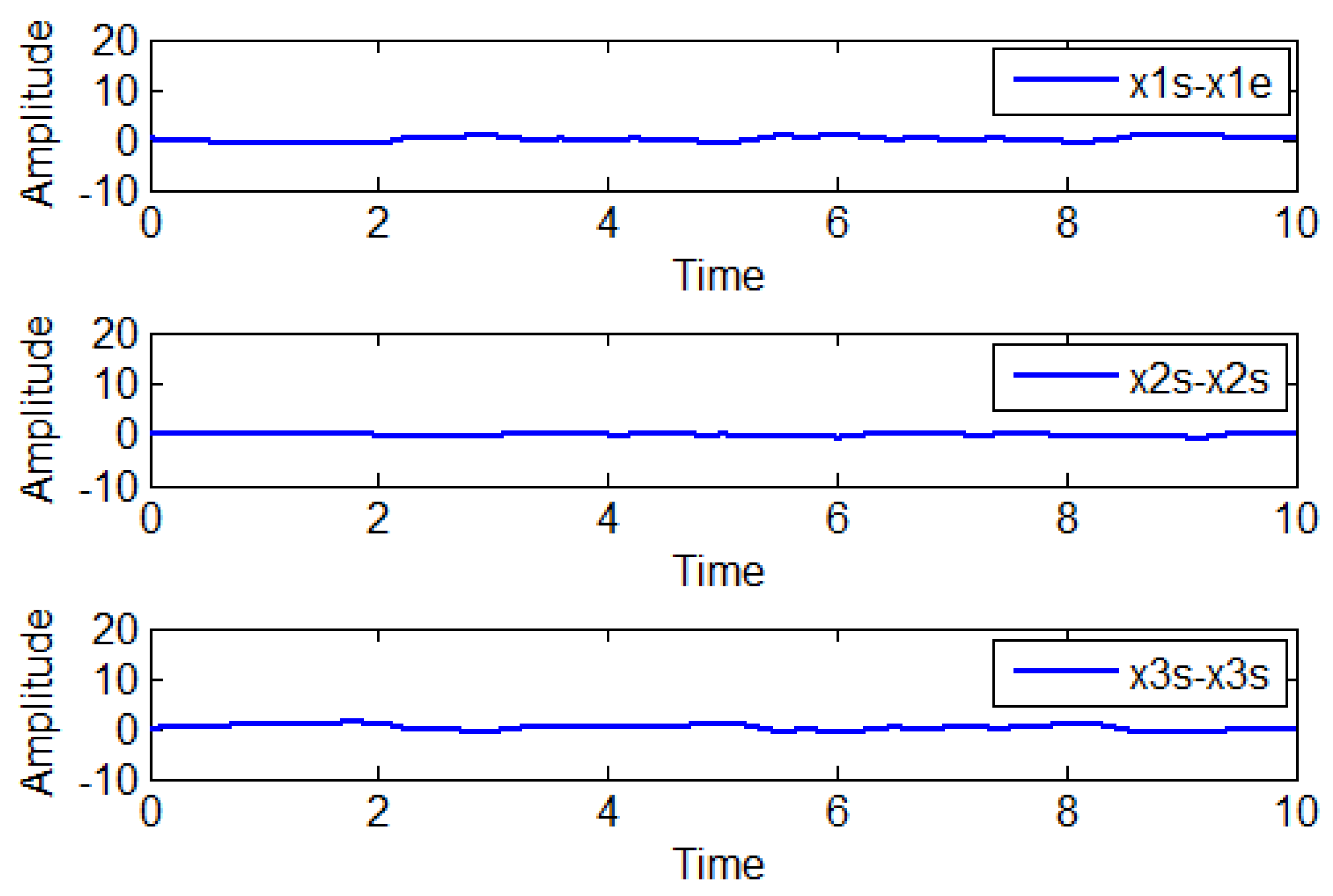
Figure 2 illustrates the estimation error dynamics of the observer designed in the paper, specifically the Fractional-Order Proportional-Integral Unknown Input Observer (FO-PIUIO). These error signals measure the difference between the estimated states and the actual system states over time.

Figure 3 shows the precision of the FO-PIUIO in the estimation of unknown inputs because real inputs (solid blue lines) and their estimates (red dashed lines) are seen to stay very close to each other along the time horizon. The resemblance shows the capability of the observer for the proper reconstruction of unknown disturbances in the system.

The benefit of the FO-PIUIO in estimating unknown inputs is its minimum deviation from actual values even in the presence of model uncertainty. The fact that the estimated unknown inputs rapidly converge to their actual values also indicates that the state augmentation method is effective in incorporating unknown inputs into the estimation. As an additional check, another subplot of error in unknown input estimation versus time can complement the visualization of observer performance.

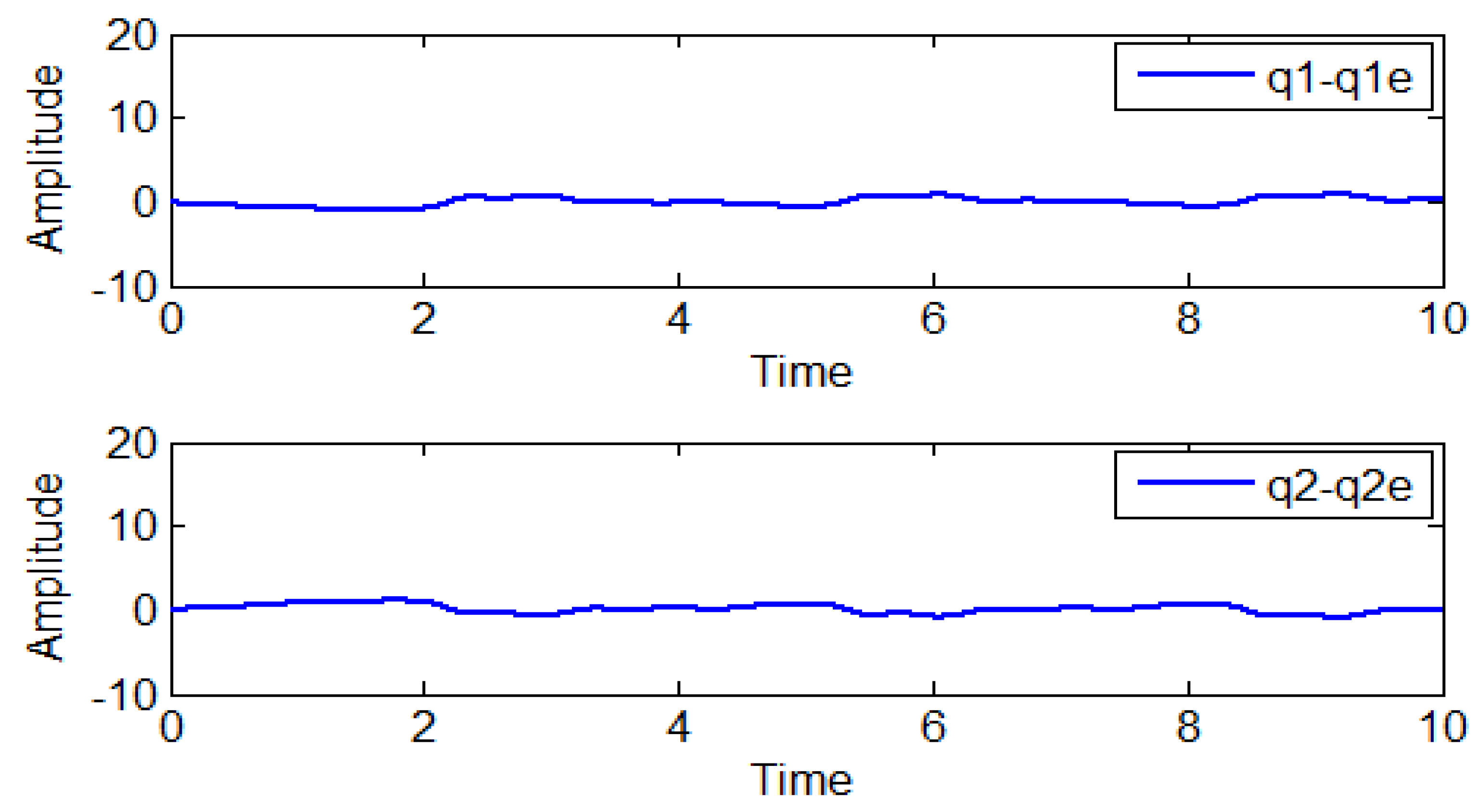
Figure 4 shows error dynamics for estimating unknown input. Plots demonstrate that unknown input estimation errors have transient behavior initially before converging to close to zero values, confirming the stability and accuracy of the observer. The fast-decreasing nature of the errors demonstrates the strong capability of the observer in rejecting disturbances and being robust to system uncertainties.

Further, the smooth and closed form of the error trajectories shows that the observer exhibits good performance with fewer oscillations, which is necessary for real-time fault detection and control issues. These findings validate the LMI-based optimization used for the synthesis of observer gains so that the estimation process is well-conditioned. The inclusion of other statistical metrics such as the variance of estimation errors may further validate the effectiveness of the suggested approach.

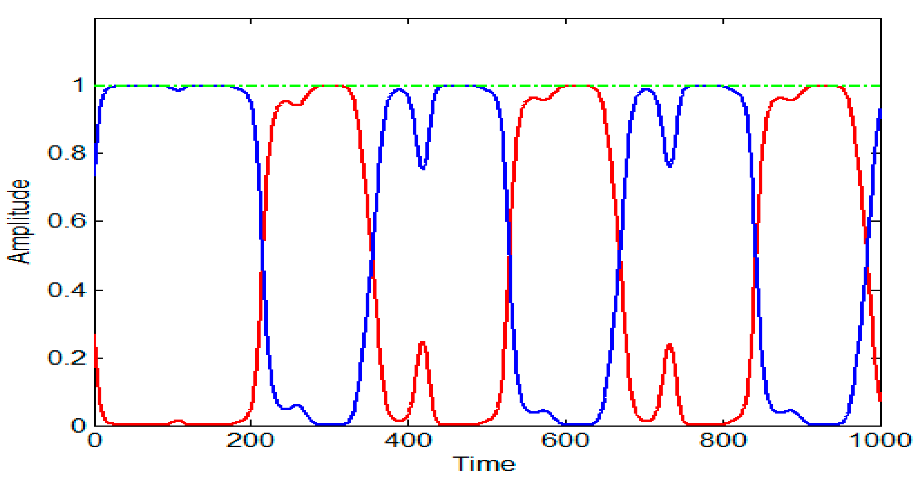
Figure 5 illustrates the evolution of the activation functions governing the switching mechanism among the fuzzy rules in the fractional-order Takagi–Sugeno (FO-TS) system. The activation functions—represented by the red, blue, and green lines—correspond respectively to the degrees of activation for fuzzy rules 1, 2, and 3. These functions determine the relative contribution of each local model in the global system behavior based on the current system state.

The observed oscillations between 0 and 1 for each activation function confirm adherence to the convexity property of fuzzy systems, ensuring that the sum of the membership values at any instant equals one. The alternating dominance of these activation levels indicates the system’s dynamic transition between operational modes in response to varying state conditions.

The simulation results clearly illustrate the better accuracy, stability, and robustness of the developed fractional-order proportional-integral unknown input observer (FO-PIUIO) in state estimation and unknown input estimation. The good agreement between the actual and estimated values, and the fast convergence of the estimation errors to near zero levels affirms the effectiveness of the state augmentation technique and LMI-based observer design. In addition, the bounded and smooth convergence of the estimation errors confirms the observer’s robustness against system uncertainties and unknown inputs. The results demonstrate the FO-PIUIO’s readiness for practical implementation in fault detection, resilient control, and dynamic system monitoring, as well as a supporting tool for safety-critical and adaptive control systems.

4.2. Discussion

The LMI conditions found in Theorems 1-2 were solved numerically using MATLAB R2014a in combination with the YALMIP interface and the SeDuMi_1_3 solvers. These tools were selected for their robustness and suitability for handling both standard and advanced linear matrix inequality (LMI) formulations. In particular, MATLAB was used for model implementation and data handling, while YALMIP and SeDuMi were employed to solve the LMI problems derived from Lyapunov-based stability analysis, including those involving Schur complement transformations and convexity-based constraints. This combination is well-suited for systems of small to moderate size (n ≤ 50 states). For larger-scale problems, further optimization strategies such as sparse matrix handling or decomposition methods may be required to ensure computational efficiency. These tools were sufficient to generate all simulations and results presented in this study.

Notwithstanding the fact that the numerical example considered in this paper predominantly deals with constant unknown inputs, the FO-PIUIO technique in principle might be adapted to accommodate time-varying unknown inputs. This becomes increasingly difficult, particularly in the field of the stability of the observer, since the error dynamics would have to be reassessed in real-time to accommodate variations of the unknown inputs. In the work that follows, we will introduce a variation of the observer to account for the nonlinear unknown inputs, especially if the higher-order derivatives of unknown inputs are not zero. This will ensure the observer remains stable and robust when the unknown inputs exhibit distinct nonlinear features. We will derive new conditions for stability to ensure the performance of the observer in such complicated scenarios.

While the method is now designed for handling relatively constant unknown inputs, the generalization to more involved and nonlinear ones remains a very significant area for future research. We are currently adapting the observer to be capable of handling these more complex scenarios with the view of handling nonlinear dynamics and ensuring stability and convergence under such scenarios.

In the example given numerically, constant unknown inputs were used for the simplification of analysis and presentation of the results. Yet this was done purely for didactic reasons, and our approach is not restricted to constant unknown inputs. It can be generalized to handle time-varying unknown inputs, although this raises further challenges, especially in proving the stability and convergence of the observer in situations of uncertainty.

We have generalized the analysis to cope with the observer’s robustness in situations where unknown inputs are time-varying and model parameters are uncertain. While the numerical example has been reduced using constant unknown inputs, we show that the FO-PIUIO method is not limited to this situation. Extensions to the method are feasible and can be generalized to more complex situations, including the handling of time-varying unknown inputs and parameter uncertainties within the model. These would involve additional stability and error dynamic considerations, so the observer remains effective across various situations.

Although the numerical example depicts the phenomenon of the FO-PIUIO method for a low-order system (order 3), it should be pointed out that it is possible to extend the method to higher-order systems, typical for real-world scenarios. However, as the dimension of the system increases, so does the computational complexity when solving the LMIs. The main challenge here is handling more complex error dynamics and solving bigger optimization systems. But the method remains viable for systems of greater dimensions, provided LMI optimization is well managed.

LMI-based synthesis provides a strong analysis for the stability and convergence of the observer. With increased system dimensions, however, the cost of LMI optimization may grow rapidly. This results in computational overhead, slowing down the process. Efficient solvers may be employed to minimize the overhead, such as SDP-based or rank-reduction-based solvers. Such an approach minimizes resource utilization without compromising the observer’s performance.

Although the numerical simulations presented in this work validate the theoretical performance of the designed observers, we know that experimental examples are essential to demonstrate the superiority of the controller when implemented in real-world scenarios. The experimental validation of the designed observer for real-world nonlinear systems, including the difficulties brought about by system noise, sensor noise, and real-time implantation constraints, will be the focus of our future work.

Future work will involve applying the proposed observer to various types of systems, such as power electronics, mechanical actuators, biomedical devices, and cyber-physical platforms. Each system imposes its own limitations, such as noise, sensor precision, actuator limitations, and real-time operation demands. For example, in power electronics, the observer will be tested under conditions of electrical noise, varying load conditions, and non-idealities in switching devices. Mechanical actuators, actuator delays, sensor drift, and friction losses will be considered. Similarly, in biomedical devices, noisy sensor measurements, limited processing, and real-time requirements will be addressed.

The implementation of the proposed observer in these systems will also entail the consideration of several practical constraints, such as sensor noise, processing limitations, and actuator delays. For instance, in cyber-physical systems, real-time communication and processing are critical, and the observer will be optimized for low-latency processing. Additionally, the observer will be formulated to cater to the specific precision requirements of each system while maintaining fault detection accuracy and state estimation reliability.

In these real applications, each system’s specificity, precision demands, and physical constraints will be taken into account responsibly. This will ensure that the proposed observer does well under various environments, managing such factors as measurement noise, sensor constraints, and processing resources. By specializing the observer in these conditions, we aspire to demonstrate its real-world superiority and robustness in real applications.

5. Conclusions

This work introduces a novel fractional-order proportional-integral unknown input observer (FO-PIUIO) design based on state augmentation for fractional-order Takagi–Sugeno (FO-TS) systems. The developed strategy offers a high accuracy of state estimation and successfully addresses the challenge posed by unknown inputs and unmeasurable premise variables (UPVs). By adopting state augmentation, the proposed method embeds the unknown inputs in an augmented system model that allows for the unbiased estimation of states and adds robustness to the observer performance. Theoretical guarantees on stability were established through Lyapunov-based conditions and linear matrix inequality (LMI) optimization, proving the asymptotic convergence of the estimation errors.

By means of numerical simulations, the observer proposed in this research exhibited improved performance in coping with unknown inputs, reducing estimation bias, and improving robustness compared to conventional observers.

The results of this work validate the effectiveness of the FO-PIUIO framework in both measurable premise variable (MPV) and unmeasurable premise variable (UPV) cases, thus highlighting its potential use in applications like fault diagnosis, control systems, and safety-critical systems.

Despite the favorable outcomes with the proposed methodology, experiments would have to be conducted to determine how effective it would be in real systems. Future experiments should aim at performing experiments on applications in robot systems, power electronics, and bio-engineering. Secondly, the use of machine learning methods like neural networks or adaptive filters would also be able to make the observer even more dynamically condition-adaptive. The creation of the FO-PIUIO framework for real-time fault detection and isolation would greatly increase its applications in safety-related applications. Also, research on the FO-PIUIO framework coupled with distributed estimation would improve its performance in large-scale networked control systems. Lastly, the reduction of the computational complexity of the LMI formulation would make this method feasible for use in real-time in complicated systems.

The suggested guidelines aim at extending the applicability, improving the stability, and optimizing the computational efficiency of the proposed observer, thus making it a more powerful tool for advanced state estimation and control of nonlinear dynamic systems.

References

1. Takagi, T.; Sugeno, M. Fuzzy identification of systems and its applications to modeling and control. IEEE Trans. Syst. Man Cybern. 1985, 15, 116–132. [Google Scholar] [CrossRef]
2. Lee, S.; Lee, S.; Lee, S. T-S fuzzy observer-based output feedback lateral control of UGVs using a disturbance observer. Drones 2024, 8, 685. [Google Scholar] [CrossRef]
3. Li, Z.; Wang, J.; Liu, H. A robust state estimator for T-S fuzzy system. IEEE Access 2020, 8, 84063–84069. [Google Scholar] [CrossRef]
4. Moodi, H.; Farrokhi, M. Robust observer-based controller design for Takagi–Sugeno systems with nonlinear consequent parts. Fuzzy Sets Syst. 2015, 273, 141–154. [Google Scholar] [CrossRef]
5. Wu, J.; Xie, H.; Li, T.; He, W.; Xi, T.; Liang, X. Design of a finite-time bounded tracking controller for time-delay fractional-order systems based on output feedback. Mathematics 2025, 13, 200. [Google Scholar] [CrossRef]
6. Phan, V.D.; Vo, C.P.; Dao, H.V.; Ahn, K.K. Robust fault-tolerant control of an electro-hydraulic actuator with a novel nonlinear unknown input observer. IEEE Access 2021, 9, 30750–30760. [Google Scholar] [CrossRef]
7. N’Doye, I.; Darouach, M.; Voos, H.; Zasadzinski, M. Design of unknown input fractional-order observers for fractional-order systems. Int. J. Appl. Math. Comput. Sci. 2013, 23, 491–500. [Google Scholar] [CrossRef]
8. Podlubny, I. Fractional Differential Equations; Academic Press: San Diego, CA, USA, 1999. [Google Scholar]
9. Magin, R. Fractional Calculus in Bioengineering; Springer: Cham, Switzerland, 2021. [Google Scholar] [CrossRef]
10. Sun, Y.; Liu, Y.; Li, L. Fuzzy adaptive control for fractional nonlinear systems with external disturbances and unknown control directions. J. Math. 2020, 2020, 6677704. [Google Scholar] [CrossRef]
11. Djeddi, A.; Dib, D.; Azar, A.T.; Abdelmalek, S. Fractional order unknown inputs fuzzy observer for TS systems. Mathematics 2019, 7, 984. [Google Scholar] [CrossRef]
12. Sabatier, J.; Moze, M.; Farges, C. LMI stability conditions for fractional order systems. Comput. Math. Appl. 2010, 59, 1594–1609. [Google Scholar] [CrossRef]
13. Boyd, S.; El Ghaoui, L.; Feron, E.; Balakrishnan, V. Linear Matrix Inequalities in System and Control Theory; SIAM: Philadelphia, PA, USA, 1994. [Google Scholar]
14. Hamdi, W.; Hammoudi, M.Y.; Boukhlouf, A. Observer design for TS fuzzy systems with unmeasurable premises. Eng. Proc. 2023, 58, 28–40. [Google Scholar] [CrossRef]
15. Niazi, M.U.B.; Cao, J.; Sun, X.; Das, A.; Johansson, K.H. Learning-based design of Luenberger observers for autonomous nonlinear systems. In Proceedings of the 2023 American Control Conference (ACC), San Diego, CA, USA, 31 May–2 June 2023. [Google Scholar] [CrossRef]
16. Djeddi, A.; Harkat, M.F. Residual structuration based on a new observer scheme for sensor fault detection and isolation. In Proceedings of the 3rd International Conference on Systems and Control, Algiers, Algeria, 29–31 October 2013; pp. 50–54. [Google Scholar] [CrossRef]
17. Djeddi, A. Diagnostic de Défauts des Systèmes non Linéaires à Base D’observateurs. Ph.D. Thesis, Université Badji Mokhtar, Annaba, Algeria, 2017. [Google Scholar]
18. Ding, S.X. Model-Based Fault Diagnosis Techniques; Springer: Berlin, Germany, 2020. [Google Scholar] [CrossRef]
19. Rebai, S.B. Advanced nonlinear fuzzy observer and robust control design for systems subject to cyber-physical attacks. Comput. Artif. Intell. 2023, 1, 409. [Google Scholar] [CrossRef]
20. Djeddi, A.; Amieur, T.; Hannachi, F.; Metatla, S.; Aouiche, A. Synthesis of fractional order fuzzy observer for a fractional order Takagi-Sugeno model with unmeasurable premise variables. Rev. Roum. Sci. Tech. Ser. Electrotech. Energ. 2024, 69, 45–50. [Google Scholar] [CrossRef]
21. Lendek, Z.; Lauber, J.; Guerra, T.M.; Babuška, R.; De Schutter, B. Adaptive observers for TS fuzzy systems with unknown polynomial inputs. Fuzzy Sets Syst. 2010, 161, 2043–2065. [Google Scholar] [CrossRef]
Figure 1. System states and their estimates.
Mathematics 13 01786 g001
Figure 2. Evolution of the state estimation errors.
Mathematics 13 01786 g002
Figure 3. Unknown inputs and their estimates.
Mathematics 13 01786 g003
Figure 4. Evolution of the unknown input estimation errors.
Mathematics 13 01786 g004
Figure 5. Activation functions.
Mathematics 13 01786 g005