The Numerical Approximation of Caputo Fractional Derivatives of Higher Orders Using a Shifted Gegenbauer Pseudospectral Method: A Case Study of Two-Point Boundary Value Problems of the Bagley–Torvik Type

Abstract

This paper introduces a novel Shifted Gegenbauer Pseudospectral (SGPS) method for approximating Caputo fractional derivatives (FDs) of an arbitrary positive order. The method employs a strategic variable transformation to express the Caputo FD as a scaled integral of the mth-derivative of the Lagrange interpolating polynomial, thereby mitigating singularities and improving numerical stability. Key innovations include the use of shifted Gegenbauer (SG) polynomials to link mth-derivatives with lower-degree polynomials for precise integration via SG quadratures. The developed fractional SG integration matrix (FSGIM) enables efficient, pre-computable Caputo FD computations through matrix–vector multiplications. Unlike Chebyshev or wavelet-based approaches, the SGPS method offers tunable clustering and employs SG quadratures in barycentric forms for optimal accuracy. It also demonstrates exponential convergence, achieving superior accuracy in solving Caputo fractional two-point boundary value problems (TPBVPs) of the Bagley–Torvik type. The method unifies interpolation and integration within a single SG polynomial framework and is extensible to multidimensional fractional problems.

1. Introduction

Fractional calculus generalizes calculus by allowing differentiation and integration to arbitrary real orders. This framework provides a powerful tool for modeling memory effects, long-range interactions, and anomalous diffusion—phenomena commonly observed in scientific and engineering applications. Unlike classical integer-order models, which assume purely local and instantaneous interactions, fractional-order models naturally incorporate non-locality and history dependence. This feature allows them to more accurately represent real-world processes such as viscoelasticity, dielectric polarization, electrochemical reactions, and subdiffusion in disordered media [1,2,3]. Moreover, fractional-order models often require fewer parameters to match or exceed the accuracy of classical models in representing complex dynamics, making them both efficient and descriptive [4].

The key advantage of FDs over classical derivatives lies in their capacity to capture hereditary characteristics and long-range temporal correlations, which are particularly relevant in biological systems [5], control systems [6], and viscoelastic materials [3]. For instance, traditional damping models use exponential kernels that decay too quickly to accurately capture certain relaxation behaviors. In contrast, fractional models employ power-law kernels, enabling them to describe slower and more realistic decay rates [7].

Among the various definitions of FDs, the Caputo FD is particularly popular due to its compatibility with classical initial and boundary conditions, which allows seamless integration with standard numerical and analytical techniques for solving fractional differential equations. Unlike the Riemann–Liouville FD, the Caputo FD defines the FD of a constant as zero, simplifying the mathematical treatment of steady-state solutions and improving the applicability of collocation methods. A prominent example of its application is the Bagley–Torvik equation, a well-known fractional differential equation involving a Caputo derivative of order 1.5. This equation models the motion of a rigid plate immersed in a viscous fluid, where the FD term represents a damping force that depends on the history of the plate’s motion. Such damping—referred to as fractional or viscoelastic damping—is commonly used to model materials exhibiting memory effects.

Recent advances in finite-time stability analysis for fractional systems (e.g., [8]) underscore the growing demand for robust numerical methods. In particular, the numerical approximation of FDs and the solution to equations such as the Bagley–Torvik equation remain active and challenging areas of research. These developments highlight the necessity of stable, efficient, and highly accurate numerical methods capable of capturing the complex dynamics inherent in fractional-order models. Several numerical studies have demonstrated that classical methods struggle to maintain accuracy or stability when adapted to fractional settings due to the singular kernel behavior of fractional integrals, especially near the origin [9]. Hence, developing dedicated fractional methods that respect the non-local structure of the problem is crucial for realistic simulations. In the following, we mention some of the key contributions to the numerical solution to the Bagley–Torvik equation using the Caputo FD: Spectral Methods: Saw and Kumar [10] proposed a Chebyshev collocation scheme for solving the fractional Bagley–Torvik equation. The Caputo FD was handled through a system of algebraic equations formed using Chebyshev polynomials and specific collocation points. Ji et al. [11] presented a numerical solution using SC polynomials. The Caputo derivative was expressed using an operational matrix of FDs, and the fractional-order differential equation was reduced to a system of algebraic equations that was solved using Newton’s method. Hou et al. [12] solved the Bagley–Torvik equation by converting the differential equation into a Volterra integral equation, which was then solved using Jacobi collocation. Ji and Hou [13] applied Laguerre polynomials to approximate the solution to the Bagley–Torvik equation. The Laplace transform was first used to convert the problem into an algebraic equation, and then, Laguerre polynomials were used for numerical inversion. Wavelet-Based Methods: Kaur et al. [14] developed a hybrid numerical method using non-dyadic wavelets for solving the Bagley–Torvik equation. Dincel [15] employed sine–cosine wavelets to approximate the solution to the Bagley–Torvik equation, where the Caputo FD was computed using the operational matrix of fractional integration. Rabiei and Razzaghi [16] introduced a wavelet-based technique, utilizing the Riemann–Liouville integral operator to transform the fractional Bagley–Torvik equation into algebraic equations. Operational Matrix Methods: Abd-Elhameed and Youssri [17] formulated an operational matrix of FDs in the Caputo sense using Lucas polynomials, and applied Tau and collocation methods to solve the Bagley–Torvik equation. Youssri [18] introduced an operational matrix approach using Fermat polynomials for solving the fractional Bagley–Torvik equation in the Caputo sense. A spectral tau method was employed to transform the problem into algebraic equations. Galerkin Methods: Izadi and Negar [19] used a local discontinuous Galerkin scheme with upwind fluxes for solving the Bagley–Torvik equation. The Caputo derivative was approximated by discretizing elementwise systems. Chen [20] proposed a fast multiscale Galerkin algorithm using orthogonal functions with vanishing moments. Spline and Finite Difference Methods: Tamilselvan et al. [21] used a second-order spline approximation for the Caputo FD and a central difference scheme for the second-order derivative term in solving the Bagley–Torvik equation. Artificial Intelligence-Based Methods: Verma and Kumar [22] employed an artificial neural network method with Legendre polynomials to approximate the solution to the Bagley–Torvik equation, where the Caputo derivative was handled through an optimization-based training process.

This work introduces a novel framework for approximating Caputo FDs of any positive orders using an SGPS method. Unlike traditional approaches, our method employs a strategic change of variables to transform the Caputo FD into a scaled integral of the mth-derivative of the Lagrange interpolating polynomial, where m is the ceiling of the fractional order $\alpha$. This transformation mitigates the singularity inherent in the Caputo derivative near zero, thereby improving numerical stability and accuracy. The numerical approximation of the Caputo FD is finally furnished by linking the mth-derivative of SG polynomials with another set of SG polynomials of lower degrees and higher parameter values whose integration can be recovered within excellent accuracies using SG quadratures. By employing orthogonal collocation and SG quadratures in barycentric form, we achieve a highly accurate, computationally efficient, and stable scheme for solving fractional differential equations under optimal parameter settings compared to classical PS methods. Furthermore, we provide a rigorous error analysis showing that the SGPS method is convergent when implemented within a semi-analytic framework, where all necessary integrals are computed analytically, and is conditionally convergent with an exponential rate of convergence for sufficiently smooth functions when performed using finite-precision arithmetic. This exponential convergence generally leads to superior accuracy compared to existing wavelet-based, operational matrix, and finite difference methods. We conduct rigorous error and convergence analyses to derive the total truncation error bound of the method and study its asymptotic behavior within double-precision arithmetic. The SGPS is highly flexible in the sense that the SG parameters associated with SG interpolation and quadratures allow for flexibility in adjusting the method to suit different types of problems. These parameters influence the clustering of collocation and quadrature points and can be tuned for optimal performance. A key contribution of this work is the development of the FSGIM. This matrix facilitates the direct computation of Caputo FDs through efficient matrix–vector multiplications. Notably, the FSGIM is constant for a given set of points and parameter values. This allows for pre-computation and storage, significantly accelerating the execution of the SGPS method. The SGPS method avoids the need for extended precision arithmetic, as it remains within the limits of double-precision computations, making it computationally efficient compared to methods that require high-precision arithmetic. The current approach is designed to handle any positive fractional order $\alpha$, making it more flexible than some existing methods that are constrained to specific fractional orders. Unlike Chebyshev polynomials (fixed clustering) or wavelets (local support), SG polynomials offer tunable clustering via their index $\lambda$, optimizing accuracy for smooth solutions, while their derivative properties enable efficient FD computation, surpassing finite difference methods in convergence rate. The efficacy of our approach is demonstrated through its application to Caputo fractional TPBVPs of the Bagley–Torvik type, where it outperforms existing numerical schemes. The method’s framework supports extension to multidimensional and time-dependent fractional PDEs through the tensor products of FSGIMs. By integrating interpolation and integration into a cohesive SG polynomial-based approach, it provides a unified solution framework for fractional differential equations.

The remainder of this paper is structured as follows. Section 2 introduces the SGPS method, providing a detailed exposition of its theoretical framework and numerical implementation. The computational complexity of the derived FSGIM is discussed in Section 3. A comprehensive error analysis of the method is carried out in Section 4, establishing its convergence properties and providing insights into its accuracy. In Section 5, we demonstrate the effectiveness of the SGPS method through a case study, focusing on its application to Caputo fractional TPBVPs of the Bagley–Torvik type. Section 6 presents a series of numerical examples, demonstrating the superior performance of the SGPS method in comparison to existing techniques. Section 7 conducts a sensitivity analysis to investigate the impact of the SG parameters on the numerical stability of the SGPS method, providing practical insights into parameter selection for relatively small interpolation and quadrature mesh sizes. Finally, Section 8 concludes the paper with a summary of our key findings and a discussion of potential future research directions.

Table 1. Table of symbols and their meanings.

Symbol	Meaning	Symbol	Meaning	Symbol	Meaning
∀	for all	${\forall }_a$	for any	${\forall }_{aa}$	for almost all
${\forall }_e$	for each	${\forall }_s$	for some	${\forall }_{rs}$	for (a) relatively small
${\forall }_{rl}$	for (a) relatively large	≪	much less than	$\neg \ll$	not much less than
≫	much greater than	∃	there exist(s)	∼	asymptotically equivalent
⪝	asymptotically less than	$\stackrel{\sim }{\le }$	asymptotically less than or equal to	≉	not sufficiently close to
$\mathfrak{C}$	set of all complex-valued functions	$\mathfrak{F}$	set of all real-valued functions	$\mathbb{C}$	set of complex numbers
$\mathbb{R}$	set of real numbers	${\mathbb{R}}_0$	set of non-negative real numbers	${\mathbb{R}}_{\mathsf{\theta }}$	set of nonzero real numbers
${\mathbb{R}}_{-1/2}^{-}$	$\{x\in \mathbb{R}:-1/2<x<0\}$	$\mathbb{Z}$	set of integers	${\mathbb{Z}}^{+}$	set of positive integers
${\mathbb{Z}}_0^{+}$	set of non-negative integers	${\mathbb{Z}}_e^{+}$	set of positive even integers	i:j:k	list of numbers from i to k with increment j
i:k	list of numbers from i to k with increment 1	$y_{1:n}$ or ${\left.y_i\right|}_{i=1:n}$	list of symbols $y_1,y_2,\dots ,y_n$	$\left\{y_{1:n}\right\}$	set of symbols $y_1,y_2,\dots ,y_n$
${\mathbb{J}}_n$	$\{0:n-1\}$	${\mathbb{J}}_n^{+}$	${\mathbb{J}}_n\cup \left\{n\right\}$	${\mathbb{N}}_n$	$\{1:n\}$
${\mathbb{N}}_{m,n}$	$\{m:n\}$	${\mathbb{G}}_n^{\lambda }$	set of GG zeros of the $(n+1)$st-degree Gegenbauer polynomial with index $\lambda >-1/2$	${\widehat{\mathbb{G}}}_n^{\lambda }$	set of SGG points in the interval $[0,1]$
${\mathsf{\Omega }}_{a,b}$	closed interval $[a,b]$	${\mathsf{\Omega }}^{\circ }$	interior of the set $\mathsf{\Omega }$	${\mathsf{\Omega }}_T$	specific interval $[0,T]$
${\mathsf{\Omega }}_{L\times T}$	Cartesian product ${\mathsf{\Omega }}_L\times {\mathsf{\Omega }}_T$	$\mathsf{\Gamma }(·)$	Gamma function	$\mathsf{\Gamma }(·,·)$	upper incomplete gamma function
$⌈.⌉$	ceiling function	${\mathfrak{I}}_{j\ge k}$	indicator (characteristic) function $\left\{\begin{array}{cc}1\hfill & \mathrm{if}j\ge k,\hfill \\ 0\hfill & \mathrm{otherwise}.\hfill \end{array}\right.$	$E_{\alpha ,\beta }\left(z\right)$	two-parameter Mittag–Leffler function
${(·)}_n$	Pochhammer symbol	$supp\left(f\right)$	support of function f	$f^{*}$	complex conjugate of f
$f_n$	$f\left(t_n\right)$	$f_{N,n}$	$f_N\left(t_n\right)$	${\mathcal{I}}_b^{\left(t\right)}h$	${\int }_0^{b}h\left(t\right)dt$
${\mathcal{I}}_{a,b}^{\left(t\right)}h$	${\int }_a^{b}h\left(t\right)dt$	${\mathcal{I}}_t^{\left(t\right)}h$	${\int }_0^{t}h(.)d(.)$	${\mathcal{I}}_b^{\left(t\right)}h-[u\left(t\right)-]$	${\int }_0^{b}h\left(u\right(t\left)\right)dt$
${\mathcal{I}}_{a,b}^{\left(t\right)}h-[u\left(t\right)-]$	${\int }_a^{b}h\left(u\right(t\left)\right)dt$	${\mathcal{I}}_{{\mathsf{\Omega }}_{a,b}}^{\left(x\right)}h$	${\int }_a^{b}h\left(x\right)dx$	${\partial }_x$	$d/dx$
${\partial }_x^n$	$d^n/d{x}^n$	${}^{c}D_x^{\alpha }f$	$\alpha$th-order Caputo FD of f at x given by ${\displaystyle {}^{c}D_x^{\alpha }f=\frac{1}{\mathsf{\Gamma }(\lceil \alpha \rceil -\alpha )}{\int }_0^x\frac{f^{(\lceil \alpha \rceil )}\left(t\right)}{{(x-t)}^{\alpha -\lceil \alpha \rceil +1}}dt}$	$\mathrm{Def}\left(\mathsf{\Omega }\right)$	space of all functions defined on $\mathsf{\Omega }$
$C^k\left(\mathsf{\Omega }\right)$	space of k times continuously differentiable functions on $\mathsf{\Omega }$	$L^p\left(\mathsf{\Omega }\right)$	Banach space of measurable functions $u\in \mathrm{Def}\left(\mathsf{\Omega }\right)$ with ${∥u∥}_{L^p}={\left({\mathcal{I}}_{\mathsf{\Omega }}{\left|u\right|}^p\right)}^{1/p}<\infty$	$L^{\infty }\left(\mathsf{\Omega }\right)$	space of all essentially bounded measurable functions on $\mathsf{\Omega }$
${∥f∥}_{L^{\infty }\left(\mathsf{\Omega }\right)}$	$L^{\infty }$ norm: ${sup}_{x\in \mathsf{\Omega }}\left|f\left(x\right)\right|=inf\{M\ge 0:|f\left(x\right)|\le M{\forall }_{aa}x\in \mathsf{\Omega }\}$	${∥·∥}_1$	$l_1$-norm	${∥·∥}_2$	Euclidean norm
${\mathcal{H}}^{k,p}\left(\mathsf{\Omega }\right)$	Sobolev space of weakly differentiable functions with integrable weak derivatives up to order k	${\mathbf{t}}_N$	${[t_{N,0},t_{N,1},\dots ,t_{N,N}]}^{\top }$	$g_{0:N}$	${[g_0,g_1,\dots ,g_N]}^{\top }$
$g^{(0:N)}$	${[g,g^{\prime },\dots ,g^{\left(N\right)}]}^{\top }$	$c^{0:N}$	$[1,c,c^2,\dots ,c^N]$	${\mathit{t}}_N^{\top }$ or $\left[t_{N,0:N}\right]$	$[t_{N,0},t_{N,1},\dots ,t_{N,N}]$
$h\left(\mathbf{y}\right)$	vector with i-th element $h\left(y_i\right)$	$\mathit{h}\left(\mathit{y}\right)$ or $h_{1:m}-[\mathit{y}-]$	${[h_1\left(\mathbf{y}\right),\dots ,h_m\left(\mathbf{y}\right)]}^{\top }$	${\mathit{y}}^{÷}$	vector of reciprocals of the elements of $\mathit{y}$
${\mathbf{O}}_n$	zero matrix of size n	${\mathbf{1}}_n$	all-ones matrix of size n	${\mathbf{I}}_n$	identity matrix of size n
${\mathbf{C}}_{n,m}$	matrix $\mathbf{C}$ of size $n\times m$	${\mathbf{C}}_n$	n-th row of matrix $\mathbf{C}$	${\mathit{1}}_n$	n-dimensional all ones column vector
${\mathit{0}}_n$	n-dimensional all-zeros column vector	${\mathbf{A}}^{\top }$ or $\mathrm{trp}\left(\mathbf{A}\right)$	transpose of matrix $\mathbf{A}$	$\mathrm{diag}\left(\mathbf{v}\right)$	diagonal matrix with $\mathbf{v}$ on the diagonal
${\mathrm{resh}}_{m,n}\left(\mathbf{A}\right)$	reshape $\mathbf{A}$ into an $m\times n$ matrix	${\mathrm{resh}}_n\left(\mathbf{A}\right)$	reshape $\mathbf{A}$ into a square matrix of size n	$\kappa \left(\mathbf{A}\right)$	condition number of $\mathbf{A}$
⊗	Kronecker product	⊙	Hadamard product	${\mathbf{A}}_{\left(r\right)}$	r-times Hadamard product of $\mathbf{A}$
${\mathbf{A}}^{\circ m}$	each entry in $\mathbf{A}$ raised to the power m	$f\left(n\right)=O\left(g\right(n\left)\right)$	$\exists n_0,c>0:0\le f\left(n\right)\le cg\left(n\right)\forall n\ge n_0$	$f\left(n\right)=o\left(g\right(n\left)\right)$	${lim}_{n\to \infty }{\displaystyle \frac{f\left(n\right)}{g\left(n\right)}}=0$

Remark: A vector is represented in print by a bold italicized symbol, while a two-dimensional matrix is represented by a bold symbol, except for a row vector whose elements form a certain row of a matrix, which is represented by a bold symbol.

and the list of acronyms display the symbols and acronyms used in the paper and their meanings. A pseudocode for the SGPS method to solve Bagley–Torvik TPBVPs is provided in Appendix A. Appendix B supports the error analysis conducted in Section 4 by providing rigorous mathematical justifications for the asymptotic order of some key terms in the error bound.

2. The SGPS Method

This section introduces the SGPS method for approximating Caputo FDs. Readers interested in obtaining a deeper understanding of Gegenbauer and SG polynomials, as well as their associated quadratures, are encouraged to consult [23,24,25,26].

Let $\alpha \in {\mathbb{R}}^{+}\setminus {\mathbb{Z}}^{+},m=⌈\alpha ⌉,f\in {\mathcal{H}}^{m,2}\left({\mathsf{\Omega }}_1\right),\left\{{\widehat{x}}_{n,0:n}^{\lambda }\right\}={\widehat{\mathbb{G}}}_n^{\lambda }$, and consider the following SGPS interpolant of f:

$$I_{n}f\left(x\right)=f_{0:n}^{\top }{\mathcal{L}}_{0:n}^{\lambda }-[x-],$$

(1)

where ${\mathcal{L}}_k^{\lambda }\left(x\right)$ is the nth-degree Lagrange interpolating polynomial in modal form defined by

$${\mathcal{L}}_k^{\lambda }\left(x\right)={\widehat{\varpi }}_k^{\lambda }\mathrm{trp}\left({\widehat{\lambda }}_{0:n}^{{\lambda }^{÷}}\right)\left({\widehat{G}}_{0:n}^{\lambda }-[{\widehat{x}}_{n,k}^{\lambda }-]\odot {\widehat{G}}_{0:n}^{\lambda }-[x-]\right),\forall k\in {\mathbb{J}}_n^{+};$$

(2)

${\widehat{\lambda }}_{0:n}^{\lambda }$ and ${\widehat{\varpi }}_{0:n}^{\lambda }$ are the normalization factors for SG polynomials and the Christoffel numbers associated with their quadratures, respectively,

$$\begin{array}{c}{\widehat{\lambda }}_j^{\lambda }={\displaystyle \frac{\pi 2^{1-4\lambda }\mathsf{\Gamma }\left(j+2\lambda \right)}{j!{\mathsf{\Gamma }}^2\left(\lambda \right)\left(j+\lambda \right)}},\\ {\widehat{\varpi }}_k^{\lambda }=1/\left[\mathrm{trp}\left({\widehat{\lambda }}_{0:n}^{{\lambda }^{÷}}\right){\left({\widehat{G}}_{0:n}^{\lambda }-[{\widehat{x}}_{n,k}^{\lambda }-]\right)}_{\left(2\right)}\right];\end{array}$$

and $\forall j,k\in {\mathbb{J}}_n^{+}$ (cf. Equations (2.6), (2.7), (2.10), and (2.12) in [23]). The matrix form of Equation (2) can be stated as

$${\mathcal{L}}_{0:n}^{\lambda }-[x-]=\mathrm{diag}\left({\widehat{\varpi }}_{0:n}^{\lambda }\right){\left({\widehat{G}}_{0:n}^{\lambda }-[x{\mathit{1}}_{n+1}-]\odot {\widehat{G}}_{0:n}^{\lambda }-[{\widehat{\mathbf{x}}}_n^{\lambda }-]\right)}^{\top } {\widehat{\lambda }}_{0:n}^{{\lambda }^{÷}}.$$

(3)

Equation (1) allows us to approximate the Caputo FD of f:

$${}^{c}D_x^{\alpha }f\approx {}^{c}D_x^{\alpha }{I}_{n}f=f_{0:n}^{\top }{}^{c}D_x^{\alpha }{\mathcal{L}}_{0:n}^{\lambda }.$$

(4)

To accurately evaluate ${}^{c}D_x^{\alpha }{\mathcal{L}}_{0:n}^{\lambda }$, we apply the following m-dependent change of variables:

$$\tau =x\left(1-y^{{\displaystyle \frac{1}{m-\alpha }}}\right),$$

which reduces ${}^{c}D_x^{\alpha }f$ to a scalar multiple of the integral of the mth-derivative of f on the fixed interval ${\mathsf{\Omega }}_1$, denoted by ${}^{E}D_x^{\alpha }f$, and defined by

$${}^{E}D_x^{\alpha }f={\displaystyle \frac{x^{m-\alpha }}{\mathsf{\Gamma }(m-\alpha +1)}}{\mathcal{I}}_1^{\left(y\right)}{f}^{\left(m\right)}-[x\left(1-y^{{\displaystyle \frac{1}{m-\alpha }}}\right)-].$$

(5)

It is easy here to show that the value of $x\left(1-y^{{\displaystyle \frac{1}{m-\alpha }}}\right)$ will always lie in the range ${\mathsf{\Omega }}_x\forall 0\le x,y\le 1$. Combining Equations (4) and (5) gives

$${}^{c}D_x^{\alpha }f\approx {\displaystyle \frac{x^{m-\alpha }}{\mathsf{\Gamma }(m-\alpha +1)}}{f}_{0:n}^{\top }{\mathcal{I}}_1^{\left(y\right)}{\mathcal{L}}_{0:n}^{\lambda ,m}-[x\left(1-y^{{\displaystyle \frac{1}{m-\alpha }}}\right)-],$$

(6)

where ${\mathcal{L}}_j^{\lambda ,m}$ denotes the mth-derivative of ${\mathcal{L}}_j^{\lambda }\forall j\in {\mathbb{J}}_n^{+}$. Substituting Equation (3) into Equation (6) yields

$$\begin{array}{c}{}^{c}D_x^{\alpha }f\approx {\displaystyle \frac{x^{m-\alpha }}{\mathsf{\Gamma }(m-\alpha +1)}}\left[\mathrm{trp}\left({\widehat{\lambda }}_{m:n}^{{\lambda }^{÷}}\right)\times \right.\end{array}$$

$$\begin{array}{c}\left.\left({\mathcal{I}}_1^{\left(y\right)}{\widehat{G}}_{m:n}^{\lambda ,m}-[\left(x-x{y}^{{\displaystyle \frac{1}{m-\alpha }}}\right){\mathit{1}}_{n+1}-]\odot {\widehat{G}}_{m:n}^{\lambda }-[{\widehat{\mathbf{x}}}_n^{\lambda }-]\right)\mathrm{diag}\left({\widehat{\varpi }}_{0:n}^{\lambda }\right)\right]f_{0:n},\end{array}$$

(7)

where ${\widehat{G}}_j^{\lambda ,m}$ denotes the mth-derivative of ${\widehat{G}}_j^{\lambda }\forall j\in {\mathbb{N}}_{m,n}$.

To efficiently evaluate Caputo FDs at arbitrary points $z_{0:M}\in {\mathsf{\Omega }}_1{\forall }_{s}M\in {\mathbb{Z}}_0^{+}$, Formula (7) can be applied iteratively within a loop. While direct implementation using a loop over the vector’s elements of ${\mathbf{z}}_M$ is possible, employing matrix operations is highly recommended for substantial performance gains. To this end, notice first that Equation (3) can be rewritten at ${\mathbf{z}}_M$ as

$${\mathcal{L}}_{0:n}^{\lambda }-[{\mathbf{z}}_M-]={\mathrm{resh}}_{n+1,M+1}\left[\mathrm{trp}\left({\widehat{\lambda }}_{0:n}^{{\lambda }^{÷}}\right)\times \right.\left({\widehat{G}}_{0:n}^{\lambda }-[{\mathbf{z}}_M\otimes {\mathit{1}}_{n+1}-]\odot {\widehat{G}}_{0:n}^{\lambda }-[{\mathit{1}}_{M+1}\otimes {\widehat{\mathbf{x}}}_n^{\lambda }-]\right)\times$$

$$\left.\left({\mathbf{I}}_{M+1}\otimes \mathrm{diag}\left({\widehat{\varpi }}_{0:n}^{\lambda }\right)\right)\right].$$

(8)

Equation (8) together with (6) yield:

$${}^{c}D_{{\mathbf{z}}_M}^{\alpha }f\approx {\displaystyle \frac{1}{\mathsf{\Gamma }(m-\alpha +1)}}\left[{{\mathbf{z}}_M}^{\circ (m-\alpha )}\odot \left({}^E\widehat{\mathbf{Q}}_n^{\alpha }{f}_{0:n}\right)\right],$$

(9)

where

$$\begin{array}{c}{}^E\widehat{\mathbf{Q}}_n^{\alpha }={\mathrm{resh}}_{n+1,M+1}^{\top }\left[\mathrm{trp}\left({\widehat{\lambda }}_{m:n}^{{\lambda }^{÷}}\right)\times \right.\\ \left({\mathcal{I}}_1^{\left(y\right)}{\widehat{G}}_{m:n}^{\lambda ,m}-[{\mathbf{z}}_M\otimes \left(\left(1-y^{{\displaystyle \frac{1}{m-\alpha }}}\right){\mathit{1}}_{n+1}\right)-]\odot {\widehat{G}}_{m:n}^{\lambda }-[{\mathit{1}}_{M+1}\otimes {\widehat{\mathbf{x}}}_n^{\lambda }-]\right)\times \\ \left.\left({\mathbf{I}}_{M+1}\otimes \mathrm{diag}\left({\widehat{\varpi }}_{0:n}^{\lambda }\right)\right)\right].\end{array}$$

With simple algebraic manipulation, we can further show that Equation (9) can be rewritten as

$${}^{c}D_{{\mathbf{z}}_M}^{\alpha }f\approx {}^E\mathbf{Q}_n^{\alpha }{f}_{0:n},$$

(10)

where

$${}^E\mathbf{Q}_n^{\alpha }={\displaystyle \frac{1}{\mathsf{\Gamma }(m-\alpha +1)}}\mathrm{diag}\left({{\mathbf{z}}_M}^{\circ (m-\alpha )}\right){}^E\widehat{\mathbf{Q}}_n^{\alpha }.$$

(11)

We refer to the $(M+1)\times (n+1)$ matrix ${}^E\mathbf{Q}_n^{\alpha }$ as “the αth-order FSGIM,” which approximates Caputo FD at the points $z_{0:M}$ using an nth-degree SG interpolant. We also refer to ${}^E\widehat{\mathbf{Q}}_n^{\alpha }$ as the “αth-order FSGIM Generator” for an obvious reason. Although the implementation of Formula (10) is straightforward, Formula (9) is slightly more stable numerically, with fewer arithmetic operations, particularly because it avoids constructing a diagonal matrix and directly applies elementwise multiplication after the matrix–vector product. Note that for $M=0$, Formulas (9) and (10) reduce to (7).

It remains now to show how to compute

$${\mathcal{I}}_1^{\left(y\right)}{\widehat{G}}_j^{\lambda ,m}-[x\left(1-y^{{\displaystyle \frac{1}{m-\alpha }}}\right)-],{\forall }_{a}j\in {\mathbb{N}}_{m:n},x\in {\mathsf{\Omega }}_1,$$

effectively. Notice first that although the integrand is defined in terms of a polynomial in x, the integrand itself is not a polynomial in y, since $1/(m-\alpha )$ is not an integer for $\alpha \in {\mathbb{R}}^{+}\setminus {\mathbb{Z}}^{+}$. Therefore, when trying to evaluate the integral symbolically, the process can be very challenging and slow. Numerical integration, on the other hand, is often more practical for such integrals because it can achieve any specified accuracy by evaluating the integrand at discrete points without requiring closed-form antiderivatives or algebraic complications. Our reliable tool for this task is the SGIM; cf. [23,25] and the references therein. The SGIM utilizes the barycentric representation of shifted Lagrange interpolating polynomials and their associated barycentric weights to approximate definite integrals effectively through matrix–vector multiplications. The SGPS quadratures constructed by these operations extend the classical Gegenbauer quadrature methods and can improve their performance in terms of convergence speed and numerical stability. An efficient way to construct the SGIM is to premultiply the corresponding GIM by half, rather than shifting the quadrature nodes, weights, and Lagrange polynomials to the target domain ${\mathsf{\Omega }}_1$, as shown earlier in [23]. In the current work, we only need the GIRV, $\mathbf{P}$, which extends the applicability of the barycentric GIM to include the boundary point 1 (cf. [24] Algorithm 6 or 7). The associated SGIRV, $\widehat{\mathbf{P}}$, can be directly generated through the formula

$$\widehat{\mathbf{P}}={\displaystyle \frac{1}{2}}\mathbf{P}.$$

Given that the construction of $\widehat{\mathbf{P}}$ is independent of the SGPS interpolant (1), we can define $\widehat{\mathbf{P}}$ using any set of SGG quadrature nodes ${\widehat{\mathbb{G}}}_{n_q}^{{\lambda }_q}{\forall }_s{n}_q\in {\mathbb{Z}}_0^{+},{\lambda }_q>-1/2$. This flexibility enables us to improve the accuracy of the required integrals without being constrained by the resolution of the interpolation grid. With this strategy, the SGIRV provides a convenient way to approximate the required integral through the following matrix–vector multiplication:

$${\mathcal{I}}_1^{\left(y\right)}{\widehat{G}}_j^{\lambda ,m}-[x-x{y}^{{\displaystyle \frac{1}{m-\alpha }}}-]\approx \widehat{\mathbf{P}}{\widehat{G}}_j^{\lambda ,m}\left(x\left(1-{\left({\widehat{\mathbf{x}}}_{n_q}^{{\lambda }_q}\right)}^{\circ {\displaystyle \frac{1}{m-\alpha }}}\right)\right),$$

(12)

${\forall }_{a}j\in {\mathbb{N}}_{m:n},x\in {\mathsf{\Omega }}_1$. We refer to a quadrature of the form (12) as the $(n_q,{\lambda }_q)$-SGPS quadrature. A remarkable property of Gegenbauer polynomials (and their shifted counterparts) is that their derivatives are essentially other Gegenbauer polynomials, albeit with different degrees and parameters, as shown by the following theorem.

Theorem 1.

The mth-derivatives of the nth-degree, λ-indexed, Gegenbauer and SG polynomials are given by

$$G_n^{\lambda ,m}\left(x\right)={\chi }_{n,m}^{\lambda }{G}_{n-m}^{\lambda +m}\left(x\right),$$

(13a)

$${\widehat{G}}_n^{\lambda ,m}\left(\widehat{x}\right)={\widehat{\chi }}_{n,m}^{\lambda }{\widehat{G}}_{n-m}^{\lambda +m}\left(\widehat{x}\right),$$

(13b)

where

$$\begin{array}{c}{\chi }_{n,m}^{\lambda }={\displaystyle \frac{2^{m}n!\mathsf{\Gamma }\left(2\lambda \right){\left(\lambda \right)}_m\mathsf{\Gamma }\left(m+n+2\lambda \right)}{\left(n-m\right)!\mathsf{\Gamma }\left(2\left(m+\lambda \right)\right)\mathsf{\Gamma }\left(n+2\lambda \right)}}\end{array},$$

$$\begin{array}{c}{\widehat{\chi }}_{n,m}^{\lambda }=2^m{\chi }_{n,m}^{\lambda }={\displaystyle \frac{n!\mathsf{\Gamma }(\lambda +1/2)\mathsf{\Gamma }(n+m+2\lambda )}{(n-m)!\mathsf{\Gamma }(n+2\lambda )\mathsf{\Gamma }(m+\lambda +1/2)}},\end{array}$$

(14)

$\forall n\ge m,x\in {\mathsf{\Omega }}_{-1,1}$, and $\widehat{x}\in {\mathsf{\Omega }}_1$.

Proof. 

Let $C_n^{\lambda }\left(x\right)$ be the nth-degree, $\lambda$-indexed Gegenbauer polynomial standardized by Szegö [27]. We shall first prove that

$$C_n^{\lambda ,m}\left(x\right)=2^m{\left(\lambda \right)}_m{C}_{n-m}^{\lambda +m}\left(x\right),\forall n\ge m,$$

(15)

where $C_j^{\lambda ,m}$ denotes the mth-derivative of $C_j^{\lambda }\forall j\in {\mathbb{N}}_{m,n}$. To this end, we shall use the well-known derivative formula of this polynomial given by the following recurrence relation:

$$C_n^{\lambda ,1}\left(x\right)=2\lambda C_{n-1}^{\lambda +1}\left(x\right),n\ge 1.$$

We will prove Equation (15) through mathematical induction on m. The base case $m=1$ holds true due to the given recurrence relation for the first derivative. Assume now that Equation (15) holds true for $m=k$, where k is an arbitrary integer such that $1<k\le n-1$. That is,

$$C_n^{\lambda ,k}\left(x\right)=2^k{\left(\lambda \right)}_k{C}_{n-k}^{\lambda +k}\left(x\right).$$

We need to show that it also holds true for $m=k+1$. Differentiating both sides of the induction hypothesis with respect to x gives

$$\begin{array}{c}{C}_n^{\lambda ,k+1}\left(x\right)={\displaystyle \frac{d}{dx}}\left[C_n^{\lambda ,k}\left(x\right)\right]={\displaystyle \frac{d}{dx}}\left[2^k{\left(\lambda \right)}_k{C}_{n-k}^{\lambda +k}\left(x\right)\right]\\ =2^k{\left(\lambda \right)}_k{\displaystyle \frac{d}{dx}}\left[C_{n-k}^{\lambda +k}\left(x\right)\right]=2^k{\left(\lambda \right)}_k·2(\lambda +k)C_{n-k-1}^{\lambda +k+1}\left(x\right)\\ =2^{k+1}{\left(\lambda \right)}_{k+1}{C}_{n-k-1}^{\lambda +k+1}\left(x\right).\end{array}$$

This shows that if the formula holds for $m=k$, it also holds for $m=k+1$. Through mathematical induction, Equation (15) holds true for all integers $m:0\le m\le n$. Formula ([28] (A.5)) and the fact that

$$C_n^{\lambda }\left(1\right)={\displaystyle \frac{\mathsf{\Gamma }(n+2\lambda )}{\mathsf{\Gamma }(n+1)\mathsf{\Gamma }\left(2\lambda \right)}},$$

immediately show that

$$G_n^{\lambda ,m}\left(x\right)=2^m{\left(\lambda \right)}_m{\displaystyle \frac{C_{n-m}^{\lambda +m}\left(1\right)}{C_n^{\lambda }\left(1\right)}}{G}_{n-m}^{\lambda +m}\left(x\right),\forall n\ge m,$$

from which Equation (13a) is derived. Formula (13b) follows from (13a) through successive application of the Chain Rule.    □

Equations (12) and (13b) bring to light the sought formula

$${\mathcal{I}}_1^{\left(y\right)}{\widehat{G}}_j^{\lambda ,m}-[x-x{y}^{{\displaystyle \frac{1}{m-\alpha }}}-]\approx {\widehat{\chi }}_{j,m}^{\lambda }\left[\widehat{\mathbf{P}}{\widehat{G}}_{j-m}^{\lambda +m}\left(x\left(1-{\left({\widehat{\mathbf{x}}}_{n_q}^{{\lambda }_q}\right)}^{\circ {\displaystyle \frac{1}{m-\alpha }}}\right)\right)\right],$$

(16)

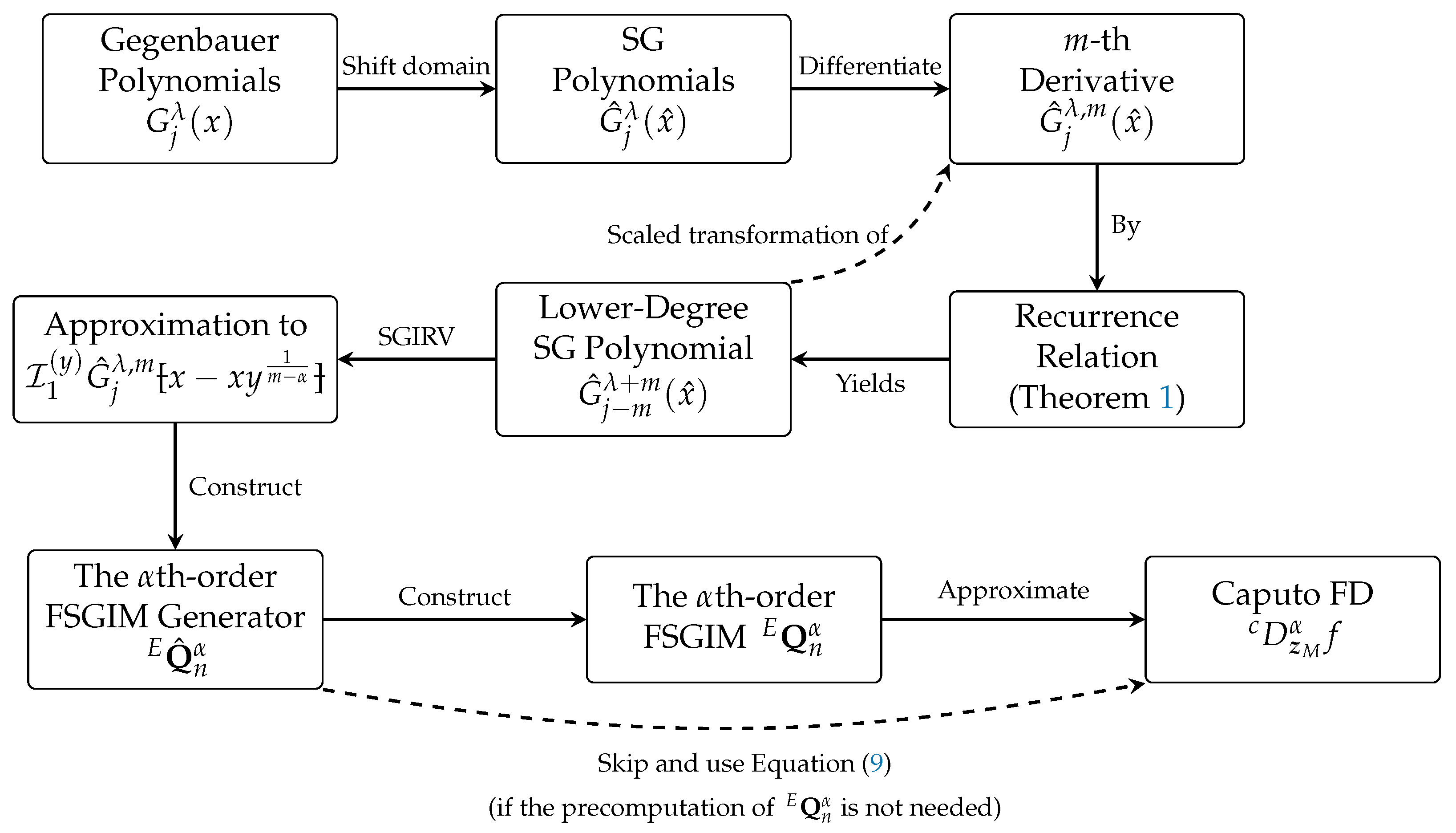
where ${\forall }_{a}j\in {\mathbb{N}}_{m:n},x\in {\mathsf{\Omega }}_1$. Figure 1 illustrates the key polynomial transformations in the SGPS method, where lower-degree SG polynomials serve as scaled transformations of the derivative terms. We denote the approximate $\alpha$th-order Caputo FD of a function at point x, computed using Equation (16) in conjunction with either Equations (9) or (10), as ${}_{n_q,{\lambda }_q}{}^{n,\lambda ,E}D_x^{\alpha }$. It is interesting to notice here that the quadrature nodes involved in the computations of the necessary integrals (16), which are required for the construction of the FSGIM ${}_{n_q,{\lambda }_q}{}^{n,\lambda ,E}D_x^{\alpha }$, are independent of the SGG points associated with the SGPS interpolant (1), and therefore, any set of SGG quadrature nodes can be used. This flexibility allows for improving the accuracy of the required integrals without being constrained by the resolution of the interpolation grid.

Figure 2 illustrates the logarithmic absolute errors of Caputo FD approximations for $f_1\left(t\right)=t^N$. These approximations utilize SG interpolants of varying parameters but consistent degrees, in conjunction with a $(15,0.5)$-SGPS quadrature. The exact Caputo FD of $f_1$ is given below:

$$\begin{array}{c}{}^{c}D_t^{\alpha }{f}_1=\left\{\begin{array}{cc}{\displaystyle \frac{N!}{\mathsf{\Gamma }(N+1-\alpha )}}{t}^{N-\alpha },\hfill & N>\alpha -1,\hfill \\ 0,\hfill & N\le \alpha -1,\hfill \end{array}\right.\forall N\in {\mathbb{Z}}_0^{+},\alpha \in {\mathbb{R}}^{+}.\end{array}$$

In all plots of Figure 2, the rapid convergence of the PS approximations is evident. Given that the SG interpolants share the same polynomial degree as the power function, and since $f_1^{(n+1)}\equiv 0$, the interpolation error vanishes, as we demonstrate later with Theorem 2 in Section 4. Consequently, the quadrature error becomes the dominant component. Theorem 4 in Section 4 further indicates that the quadrature error vanishes for $n<n_q+m+1$, which elucidates the high accuracy achieved by the SGPS method in all four plots when n is sufficiently less than $n_q+m+1$ in many cases, leading to a near-machine epsilon level of the total error. While the error analysis in Section 4 predicts the collapse of the total error when $n\le n_q+m$ under exact arithmetic, the limitations of finite-digit arithmetic often prevent this, frequently necessitating an increase in $n_q$ by one unit or more, especially when varying ${\lambda }_q$, for effective total error collapse. In Subplot 1, with $n_q=4$, an nth-degree SG interpolant sufficiently approximates the Caputo FD of the power function $t^n$ to within machine precision for $2\le n\le 5$. The error curves exhibit plateaus in this range, with slight fluctuations for specific $\lambda$ values, attributed to accumulated round-off errors as the approximation approaches machine precision. For $6\le n\le 10$, the total error becomes predominantly the quadrature error and remains relatively stable around ${10}^{-4}$. Notably, the error profiles remain consistent for $6\le n\le 10$ despite variations in $\lambda$. Altering ${\lambda }_q$ while keeping $\lambda$ constant can significantly impact the error, as shown in the upper right plot. Specifically, the error generally decreases with decreasing ${\lambda }_q$ values, with the exception of ${\lambda }_q=0.5$, where the error reaches its minimum. The lower left plot demonstrates the exponential decay of the error with increasing values of $n_q$, with the error decreasing by approximately two orders of magnitude for every two-unit increase in $n_q$. The lower right plot presents a comparison between the SGPS method and MATLAB’s “integral” function, employing the tolerance parameters RelTol = AbsTol $={10}^{-15}$. The SGPS method achieves near-machine-precision accuracy with the parameter values $\lambda ={\lambda }_q=0.5$ and $n_q=12$, outperforming MATLAB’s integral function by nearly two orders of magnitude in certain cases. The method achieves near-machine-epsilon precision with relatively coarse grids, demonstrating notable stability through consistent error trends.

Figure 3 further shows the logarithmic absolute errors of the Caputo FD approximations of the function $f_2\left(t\right)=e^{\beta t}:\beta \in {\mathbb{R}}^{+}$ using SG interpolants of various parameters and a $(15,0.5)$-SGPS quadrature. The exact Caputo FD of $f_2$ is given below:

$${}^{c}D_t^{\alpha }{f}_2=\sum _{k=0}^{\infty }{\displaystyle \frac{{\beta }^{k+m}{t}^{-\alpha +k+m}}{\mathsf{\Gamma }\left(k+m-\alpha +1\right)}}={\beta }^{\alpha }{t}^{-\alpha }{E}_{1,\alpha -m+1}\left(\beta t\right).$$

The figure illustrates the rapid convergence of the proposed PS approximations. Specifically, across the parameter range $\lambda \in \{-0.2,-0.1,0,0.5,1,2\}$, the logarithmic absolute errors exhibit a consistent decrease as the degree of the Gegenbauer interpolant increases. This trend underscores the improved accuracy of higher-degree interpolants in approximating the Caputo FD up to a defined precision threshold. For lower degrees (n), the error reduction is more enunciated as $\lambda$ decreases, indicating that other members of the SG polynomial family, associated with negative $\lambda$ values, exhibit superior convergence rates in these cases. For higher degrees (n), the errors converge to a stable accuracy level irrespective of the $\lambda$ value, highlighting the robustness of higher-degree interpolants in accurately approximating the Caputo FD. The near-linear error profiles observed in the plots confirm the exponential convergence of the PS approximations, with convergence rates modulated by the parameter selections, as detailed in Section 4.

3. Computational Complexity

In this section, we provide a computational complexity analysis of constructing ${}^E\mathbf{Q}_n^{\alpha }$, incorporating the quadrature approximation (16). The analysis is based on the key matrix operations involved in the construction process, which we analyze individually as follows: Observe from Equation (11) that the term ${{\mathbf{z}}_M}^{\circ (m-\alpha )}$ involves raising each element of an $(M+1)$-dimensional vector to the power $(m-\alpha )$, which requires $O\left(M\right)$ operations. Constructing ${}^E\mathbf{Q}_n^{\alpha }$ from ${}^E\widehat{\mathbf{Q}}_n^{\alpha }$ involves diagonal scaling by $\mathrm{diag}\left({{\mathbf{z}}_M}^{\circ (m-\alpha )}\right)$, which requires another $O\left(Mn\right)$ operation. The matrix ${}^E\widehat{\mathbf{Q}}_n^{\alpha }$ is constructed using several matrix multiplications and elementwise operations. For each entry of ${\mathbf{z}}_M$, the dominant steps include the following:

• The computation of ${\widehat{G}}_{m:n}^{\lambda }$. Using the three-term recurrence equation

  $$(n+2\alpha ){\widehat{G}}_{n+1}^{\left(\lambda \right)}\left(\widehat{x}\right)=2(n+\alpha )(2\widehat{x}-1){\widehat{G}}_n^{\left(\lambda \right)}\left(\widehat{x}\right)-n{\widehat{G}}_{n-1}^{\left(\lambda \right)}\left(\widehat{x}\right),$$
  $\forall n\in {\mathbb{Z}}^{+}$, starting with ${\widehat{G}}_0^{\left(\lambda \right)}\left(\widehat{x}\right)=1$ and ${\widehat{G}}_1^{\left(\lambda \right)}\left(\widehat{x}\right)=2\widehat{x}-1$, we find that each polynomial evaluation requires $O\left(1\right)$ per point, as the number of operations remains constant regardless of the value of n. Since the polynomial evaluation is required for polynomials up to degree n, this requires $O\left(n\right)$ operations per point. The computations of ${\widehat{G}}_{m:n}^{\lambda }-[{\widehat{\mathbf{x}}}_n^{\lambda }-]$ therefore require $O\left(n^2\right)$ operations.
• The quadrature (16) involves evaluating a polynomial at transformed nodes. The cost of calculating ${\widehat{\chi }}_{j,m}^{\lambda }$ depends on the chosen methods for computing factorials and the Gamma function. It can be considered a constant overhead for each evaluation of the Equation (14). The computation of ${\left({\widehat{\mathbf{x}}}_{n_q}^{{\lambda }_q}\right)}^{\circ {\displaystyle \frac{1}{m-\alpha }}}$ involves raising each element of the column vector ${\widehat{\mathbf{x}}}_{n_q}^{{\lambda }_q}$ to the power $1/(m-\alpha )$. The cost here is linear in $(n_q+1)$, as each element requires a single exponentiation operation. Since we need to evaluate the polynomial at $n_q+1$ points, the total cost for this step is $O\left(n_q\right)$. The cost of the matrix–vector multiplication is also linear in $n_q+1$. Therefore, the computational cost of this step is $O\left(n_q\right)$ for each $j\in {\mathbb{N}}_{m:n}$. The overall cost, if we consider all polynomial functions involved in this step, is thus $O\left(n{n}_q\right)$.
• The Hadamard product introduces another $O\left(n^2\right)$ operations.
• The evaluation of ${\widehat{\lambda }}_{m:n}^{{\lambda }^{÷}}$ requires $O\left(n\right)$ operations, and the product of $\mathrm{trp}\left({\widehat{\lambda }}_{m:n}^{{\lambda }^{÷}}\right)$ according to the result from the Hadamard product requires $O\left(n^2\right)$ operations.
• The final diagonal scaling $\mathrm{diag}\left({\widehat{\varpi }}_{0:n}^{\lambda }\right)$ contributes $O\left(n\right)$.

Summing the dominant terms, the overall computational complexity of constructing ${}^E\mathbf{Q}_n^{\alpha }$ is of $O\left(n(n+n_q)\right)$ per entry of ${\mathbf{z}}_M$. We therefore expect the total number of operations required to construct the matrix ${}^E\mathbf{Q}_n^{\alpha }$ for all entries of ${\mathbf{z}}_M$ to be of $O\left(Mn(n+n_q)\right)$.

Remark 1.

The construction runtime of the FSGIM matrix ${}^E\mathbf{Q}_n^{\alpha }$ (size $(M+1)\times (n+1)$) used by the SGPS method scales as $O\left(Mn(n+n_q)\right)$, where n is the interpolant degree, M is the number of evaluation points, and $n_q$ is the highest degree of the Gegenbauer polynomial used to construct the quadrature rule. For large n and M, the FSGIM requires $O\left(Mn\right)$ storage. While this remains manageable in double-precision arithmetic, precomputation of the FSGIM offsets runtime costs, making the method practical for moderate-scale problems. For sufficiently smooth solutions, the chosen quadrature parameter $n_q$ can often be smaller than n without sacrificing accuracy, as the integrands are well approximated by low-degree polynomials. This reduces the dominant $O\left(Mn{n}_q\right)$ term in the runtime and further improves the efficiency.

4. Error Analysis

The following theorem defines the truncation error of the $\alpha$th-order SGPS quadrature (10) associated with the $\alpha$th-order FSGIM ${}^E\mathbf{Q}_n^{\alpha }$ in closed form.

Theorem 2.

Let $n\ge m-1$, and suppose that $f\in C^{n+1}\left({\mathsf{\Omega }}_1\right)$ is approximated by the SGPS interpolant (1). Also, assume that the integrals

$${\mathcal{I}}_1^{\left(y\right)}{\widehat{G}}_{m:n}^{\lambda ,m}-[x\left(1-y^{{\displaystyle \frac{1}{m-\alpha }}}\right)-],$$

(17)

are computed exactly ${\forall }_{a}x\in {\mathsf{\Omega }}_1$. Then, $\exists \xi =\xi \left(x\right)\in {\mathsf{\Omega }}_1^{\circ }$ such that the truncation error, ${}^{\alpha }T_n^{\lambda }(x,\xi )$, in the Caputo FD approximation (7) is given by

$${}^{\alpha }T_n^{\lambda }(x,\xi )={}^{\alpha }\eta _n^{\lambda }{f}^{(n+1)}\left(\xi \right){\mathcal{I}}_x^{\left(\tau \right)}{\displaystyle \frac{{\widehat{G}}_{n+1-m}^{\lambda +m}}{{(x-\tau )}^{\alpha +1-m}}},$$

(18)

where

$${}^{\alpha }\eta _n^{\lambda }={\displaystyle \frac{\sqrt{\pi }{2}^{-2\lambda -2n-1}\mathsf{\Gamma }\left(m+n+2\lambda +1\right)}{(n-m+1)!\mathsf{\Gamma }\left(m-\alpha \right)\mathsf{\Gamma }\left(m+\lambda +\frac{1}{2}\right)\mathsf{\Gamma }\left(n+\lambda +1\right)}}.$$

Proof. 

The Lagrange interpolation error associated with the SGPS interpolation (1) is given below:

$$f\left(x\right)=I_{n}f\left(x\right)+{\displaystyle \frac{f^{(n+1)}\left(\xi \right)}{(n+1)!{\widehat{K}}_{n+1}^{\lambda }}}{\widehat{G}}_{n+1}^{\lambda }\left(x\right),$$

where ${\widehat{K}}_n^{\lambda }$ is the leading coefficient of the nth-degree, $\lambda$-indexed SG polynomial (cf. Equation (4.12) in [23]). Applying Caputo FD on both sides of the equation gives the truncation error associated with Formula (7) in the following form:

$$\begin{array}{c}{}^{\alpha }T_n^{\lambda }(x,\xi )={\displaystyle \frac{f^{(n+1)}\left(\xi \right)}{(n+1)!{\widehat{K}}_{n+1}^{\lambda }}}{}^{c}D_x^{\alpha }{\widehat{G}}_{n+1}^{\left(\lambda \right)}\end{array}$$

$$\begin{array}{c}={\displaystyle \frac{f^{(n+1)}\left(\xi \right)}{(n+1)!{\widehat{K}}_{n+1}^{\lambda }\mathsf{\Gamma }(m-\alpha )}}{\mathcal{I}}_x^{\left(\tau \right)}{\displaystyle \frac{{\widehat{G}}_{n+1}^{(\lambda ,m)}}{{(x-\tau )}^{\alpha +1-m}}}.\end{array}$$

(19)

The proof is established by substituting Formula (13b) into (19).    □

For the theoretical truncation error in Equation (18), we assume that the integrals in Equation (17) are evaluated exactly. In practice, however, these integrals are approximated using SGPS quadratures, with the corresponding quadrature errors analyzed in Theorems 4 and 5, as discussed later in this section.

The following theorem marks the truncation error bound associated with Theorem 2.

Theorem 3.

Suppose that the assumptions of Theorem 2 hold true. Then, the truncation error ${}^{\alpha }T_n^{\lambda }(x,\xi )$ is asymptotically bounded above by

$$\left|{}^{\alpha }T_n^{\lambda }(x,\xi )\right|⪝{\mathcal{A}}_{n+1}{\widehat{\vartheta }}_{m,\lambda }{2}^{-2\lambda -2n}{n}^{\lambda +m}{\forall }_{rl}n,$$

(20)

where ${\mathcal{A}}_n={∥f^{\left(n\right)}∥}_{L^{\infty }\left({\mathsf{\Omega }}_1\right)}$ and

$$\begin{array}{c}{\widehat{\vartheta }}_{m,\lambda }={\displaystyle \frac{1}{\sqrt{e}}}{\left(\lambda +m-{\displaystyle \frac{1}{2}}\right)}^{-\lambda -m}{\left(\left(\lambda +m-{\displaystyle \frac{1}{2}}\right)sinh\left({\displaystyle \frac{1}{\lambda +m-\frac{1}{2}}}\right)\right)}^{{\displaystyle \frac{1}{4}}\left(-2\lambda -2m+1\right)}.\end{array}$$

Proof. 

Since $\lambda +m>3/2>0$, Equation (4.29a) in [23] shows that ${∥{\widehat{G}}_{n+1-m}^{\lambda +m}∥}_{L^{\infty }\left({\mathsf{\Omega }}_1\right)}=1$. Thus,

$$\left|{\mathcal{I}}_x^{\left(\tau \right)}{\displaystyle \frac{{\widehat{G}}_{n+1-m}^{\lambda +m}}{{(x-\tau )}^{\alpha +1-m}}}\right|\le {\mathcal{I}}_x^{\left(\tau \right)}{(x-\tau )}^{m-\alpha -1}={\displaystyle \frac{x^{m-\alpha }}{m-\alpha }}\le {\displaystyle \frac{1}{m-\alpha }},$$

(21)

according to the Mean Value Theorem for Integrals. Notice also that $\mathsf{\Gamma }\left(z\right)>1/z\forall z\in {\mathsf{\Omega }}_1^{\circ }$. Combining this elementary inequality with the sharp inequalities of the Gamma function ([25] Inequality (96)) implies that

$$\begin{array}{c}\left|{}^{\alpha }\eta _n^{\lambda }\right|<{\displaystyle \frac{1}{\sqrt{e}}}\left(m-\alpha \right){\left(\lambda +m-{\displaystyle \frac{1}{2}}\right)}^{-\lambda -m}{2}^{-2\lambda -2n-{\displaystyle \frac{3}{2}}}{\left(\lambda +n\right)}^{-\lambda -n-{\displaystyle \frac{1}{2}}}\times \end{array}$$

$$\begin{array}{c}{\left(\left(\lambda +m-{\displaystyle \frac{1}{2}}\right)sinh\left({\displaystyle \frac{1}{\lambda +m-\frac{1}{2}}}\right)\right)}^{{\displaystyle \frac{1}{4}}\left(-2\lambda -2m+1\right)}{\left(2\lambda +m+n\right)}^{2\lambda +m+n+{\displaystyle \frac{1}{2}}}\times \end{array}$$

$$\begin{array}{c}\left({\displaystyle \frac{1}{1620{\left(2\lambda +m+n\right)}^5}}+1\right){\left(\left(\lambda +n\right)sinh\left({\displaystyle \frac{1}{\lambda +n}}\right)\right)}^{{\displaystyle \frac{1}{2}}\left(-\lambda -n\right)}\times \end{array}$$

$$\begin{array}{c}{\left(\left(2\lambda +m+n\right)sinh\left({\displaystyle \frac{1}{2\lambda +m+n}}\right)\right)}^{\lambda +{\displaystyle \frac{m+n}{2}}}\sim {\vartheta }_{\alpha ,\lambda }{2}^{-2\lambda -2n-{\displaystyle \frac{3}{2}}}{n}^{\lambda +m}{\forall }_{rl}n,\end{array}$$

(22)

where ${\vartheta }_{\alpha ,\lambda }=(m-\alpha ){\widehat{\vartheta }}_{m,\lambda }$. The required asymptotic Formula (20) is derived by combining the asymptotic Formula (22) with In Equation (21).    □

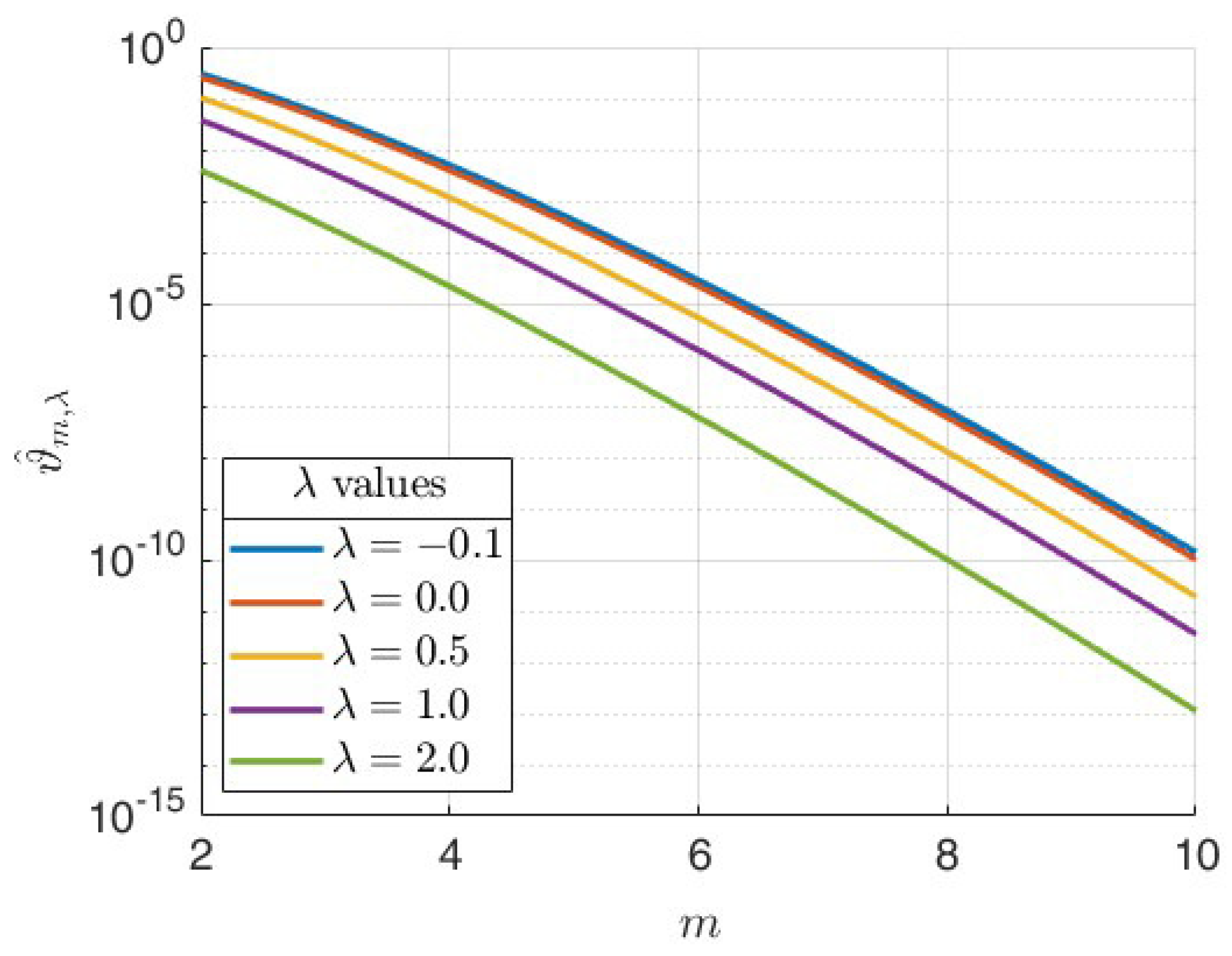
Since the dominant term in the asymptotic bound (20) is $2^{-2\lambda -2n}$, the truncation error exhibits exponential decay as $n\to \infty$. Notice also that increasing $\alpha$ while keeping $\lambda$ fixed and keeping n sufficiently large leads to an increase in m, which, in turn, affects two factors: (i) the polynomial term $n^{\lambda +m}$ grows, which slightly slows convergence, and (ii) the prefactor ${\widehat{\vartheta }}_{m,\lambda }\sim e^{-1/2}{m}^{-(\lambda +m)}{\forall }_{rl}m$, which decreases exponentially, reducing the error; cf. Figure 4. Despite the polynomial growth of the former factor, the exponential decay term $2^{-2n}$ dominates. Now, let us consider the effect of changing $\lambda$ while keeping $\alpha$ fixed and n large enough. If we increase $\lambda$ gradually, the term $2^{-2\lambda }$ will exhibit exponential decay, and the prefactor ${\widehat{\vartheta }}_{m,\lambda }\sim e^{-1/2}{\lambda }^{-(\lambda +m)}{\forall }_{rl}\lambda$ will also decrease exponentially, further reducing the error. The polynomial term $n^{\lambda +m}$, on the other hand, will increase, slightly increasing the error. Although the polynomial term $n^{\lambda +m}$ grows and slightly increases the error, the dominant exponential decay effects from both $2^{-2\lambda }$ and the prefactor ${\widehat{\vartheta }}_{m,\lambda }$ ensure that the truncation error decreases significantly as $\lambda$ increases. Hence, increasing $\lambda$ leads to faster decay of the truncation error. This analysis shows that for ${\forall }_{rl}n$, increasing $\alpha$ slightly increases the error bound due to polynomial growth but does not affect exponential convergence. Furthermore, increasing $\lambda$ generally improves convergence, since the exponential decay dominates the polynomial growth. In fact, one can see this last remark from two other viewpoints:

(i)

${\forall }_{rl}n/(m-1),supp\left({\widehat{G}}_{n+1-m}^{\lambda +m}\right)\to \{0,1\}{\forall }_{rl}\lambda$, and the truncation error ${}^{\alpha }T_n^{\lambda }\to 0$ accordingly.

(ii)

$\forall \lambda \in {\mathbb{R}}^{+},supp\left({\widehat{G}}_j^{\lambda ,m}\right)\to \{0,1\}$, as $j/m\to \infty$. Consequently, the integrals (17) collapse $\forall {\widehat{G}}_k^{\lambda ,m}:m<k\le n,k\gg m$, indicating faster convergence rates in the Caputo FD approximation (7).

In all cases, choosing a sufficiently large n ensures overall exponential convergence. It is important to note that these observations are based on the asymptotic behavior of the error upper bound as $n\to \infty$, assuming the SGPS quadrature is computed exactly.

Beyond the convergence considerations mentioned above, we highlight two important numerical stability issues related to this analysis:

(i)

A small buffer parameter $\epsilon$ is often introduced to offset the instability of the SG interpolation near $\lambda =-1/2$, where SG polynomials grow rapidly for increasing orders [23].

(ii)

As $\lambda$ increases, the SGG nodes ${\widehat{x}}_{n,0:n}^{\lambda }$ cluster more toward the center of the interval. This means that the SGPS interpolation rule (1) relies more on extrapolation than interpolation, making it more sensitive to perturbations in the function values and amplifying numerical errors. This consideration reveals that, although increasing $\lambda$ theoretically improves the convergence rate, it can introduce numerical instability due to increased extrapolation effects. Therefore, when selecting $\lambda$, one must balance convergence speed against numerical stability considerations to ensure accurate interpolation computations. This aligns well with the widely accepted understanding that, for sufficiently smooth functions and sufficiently large spectral expansion terms, the truncated expansion in the SC quadrature (corresponding to $\lambda =0$) is optimal in the $L^{\infty }$-norm for definite integral approximations; cf. [28] and the references therein.

In the following, we study the truncation error of the quadrature Formula (16) and how its outcomes add up to the above analysis.

Theorem 4.

Let $j\in {\mathbb{N}}_{m:n},x\in {\mathsf{\Omega }}_1$, and assume that ${\widehat{G}}_{j-m}^{\lambda +m}\left(x-x{y}^{{\displaystyle \frac{1}{m-\alpha }}}\right)$ is interpolated by the SG polynomials with respect to the variable y at the SGG nodes ${\widehat{x}}_{n_q,0:n_q}^{{\lambda }_q}$. Then, $\exists \eta =\eta \left(y\right)\in {\mathsf{\Omega }}_1^{\circ }$ such that the truncation error, ${\mathfrak{T}}_{j,n_q}^{{\lambda }_q}\left(\eta \right)$, in the quadrature approximation (16) is given by

$$\begin{array}{c}{\mathfrak{T}}_{j,n_q}^{{\lambda }_q}\left(\eta \right)={\displaystyle \frac{{(-1)}^{n_q+1}{\widehat{\chi }}_{j-m,n_q+1}^{\lambda +m}}{(n_q+1)!{\widehat{K}}_{n_q+1}^{{\lambda }_q}}}{\left({\displaystyle \frac{x}{m-\alpha }}\right)}^{n_q+1}{\eta }^{{\displaystyle \frac{(n_q+1)(1-m+\alpha )}{m-\alpha }}}\times \end{array}$$

$$\begin{array}{c}{\widehat{G}}_{j-m-n_q-1}^{\lambda +m+n_q+1}\left(x-x{\eta }^{{\displaystyle \frac{1}{m-\alpha }}}\right){\mathcal{I}}_1^{\left(y\right)}{\widehat{G}}_{n_q+1}^{{\lambda }_q}·{\mathfrak{I}}_{j\ge m+n_q+1}.\end{array}$$

(23)

Proof. 

Theorem 4.1 in [23] immediately shows that

$$\begin{array}{c}{\mathfrak{T}}_{j,n_q}^{{\lambda }_q}\left(\eta \right)={\displaystyle \frac{1}{(n_q+1)!{\widehat{K}}_{n_q+1}^{{\lambda }_q}}}{\left[{\partial }_y^{n_q+1}{\widehat{G}}_{j-m}^{\lambda +m}\left(x-x{y}^{{\displaystyle \frac{1}{m-\alpha }}}\right)\right]}_{y=\eta }{\mathcal{I}}_1^{\left(y\right)}{\widehat{G}}_{n_q+1}^{{\lambda }_q}\end{array}$$

$$\begin{array}{c}={\displaystyle \frac{{(-1)}^{n_q+1}}{(n_q+1)!{\widehat{K}}_{n_q+1}^{{\lambda }_q}}}{\left({\displaystyle \frac{x}{m-\alpha }}\right)}^{n_q+1}{\eta }^{{\displaystyle \frac{(n_q+1)(1-m+\alpha )}{m-\alpha }}}{\widehat{G}}_{j-m}^{\lambda +m,n_q+1}\left(x-x{\eta }^{{\displaystyle \frac{1}{m-\alpha }}}\right){\mathcal{I}}_1^{\left(y\right)}{\widehat{G}}_{n_q+1}^{{\lambda }_q},\end{array}$$

(24)

according to the Chain Rule. The error bound (23) is accomplished by substituting Formula (13b) into (24). The proof is completed by further realizing that

$${\widehat{G}}_{j-m}^{\lambda +m,n_q+1}\left(x-x{\eta }^{{\displaystyle \frac{1}{m-\alpha }}}\right)={\left.{\partial }_{\tau }^{n_q+1}{\widehat{G}}_{j-m}^{\lambda +m}\left(\tau \right)\right|}_{\tau =x-x{\eta }^{{\displaystyle \frac{1}{m-\alpha }}}}=0,$$

$\forall j<m+n_q+1$.    □

The truncation error analysis of the quadrature approximation (16) hinges on understanding the interplay between the parameters $j,n_q,m,\lambda$ and ${\lambda }_q$. While Theorem 4 provides an exact error expression, the next theorem establishes a rigorous asymptotic upper bound, revealing how the error scales with these parameters.

Theorem 5.

Let the assumptions of Theorem 4 hold true. Then, the truncation error, ${\mathfrak{T}}_{j,n_q}^{{\lambda }_q}\left(\eta \right)$, in the quadrature approximation (16) is bounded above by

$$\begin{array}{c}\left|{\mathfrak{T}}_{j,n_q}^{{\lambda }_q}\left(\eta \right)\right|⪝B_m^{\lambda ,{\lambda }_q}{2}^{-2n_q}{\left(j-m-n_q\right)}^{-j+m+n_q+{\displaystyle \frac{1}{2}}}{j}^{-2\lambda -2m+1}\times \end{array}$$

$$\begin{array}{c}{\left(j+n_q\right)}^{j+2\lambda +m+n_q+{\displaystyle \frac{1}{2}}}{n}_q^{-2n_q-m-\lambda +{\lambda }_q-{\displaystyle \frac{5}{2}}}{\left({\displaystyle \frac{x}{m-\alpha }}\right)}^{n_q+1}{\eta }^{{\displaystyle \frac{(n_q+1)(1-m+\alpha )}{m-\alpha }}}\times \end{array}$$

$$\begin{array}{c}{{\rm Y}}_{D^{{\lambda }_q}}\left(n_q\right){\mathfrak{I}}_{j\ge m+n_q+1},\end{array}$$

(25)

${\forall }_{rl}{n}_q$, where

$${{\rm Y}}_{D^{{\lambda }_q}}\left(n_q\right)=\left\{\begin{array}{c}1,{\lambda }_q\in {\mathbb{R}}_0^{+},\hfill \\ D^{{\lambda }_q}{n}_q^{-{\lambda }_q},{\lambda }_q\in {\mathbb{R}}_{-1/2}^{-},\hfill \end{array}\right.$$

where $D^{{\lambda }_q}>1$ is a constant dependent on ${\lambda }_q$, and $B_m^{\lambda ,{\lambda }_q}$ is a constant dependent on $m,\lambda$, and ${\lambda }_q$.

Proof. 

Lemma 5.1 in [26] shows that

$${∥{\widehat{G}}_k^{\gamma }∥}_{L^{\infty }\left({\mathsf{\Omega }}_1\right)}=\left\{\begin{array}{c}1,k\in {\mathbb{Z}}_0^{+},\gamma \in {\mathbb{R}}_0^{+},\hfill \\ {\sigma }^{\gamma }{k}^{-\gamma },\gamma \in {\mathbb{R}}_{-1/2}^{-},k\to \infty ,\hfill \end{array}\right.$$

(26)

where ${\sigma }^{\gamma }>1$ is a constant dependent on $\gamma$. Therefore,

$$\left|{\widehat{G}}_{j-m-n_q-1}^{\lambda +m+n_q+1}\left(x-x{\eta }^{{\displaystyle \frac{1}{m-\alpha }}}\right)\right|\le 1,$$

since $\lambda +m+n_q+1>0$. Moreover, Formula (14) and the definition of ${\widehat{K}}_{n_q}^{{\lambda }_q}$ (see p.g. 103 of [26]) show that

$$\begin{array}{c}{\displaystyle \frac{{\widehat{\chi }}_{j-m,n_q+1}^{\lambda +m}}{(n_q+1)!{\widehat{K}}_{n_q+1}^{{\lambda }_q}}}={\displaystyle \frac{2^{-2n_q-1}\mathsf{\Gamma }\left({\lambda }_q+1\right)\left(j-m\right)!}{\mathsf{\Gamma }\left(2{\lambda }_q+1\right)\mathsf{\Gamma }\left(n_q+2\right)\mathsf{\Gamma }\left(n_q+{\lambda }_q+1\right)}}\times \end{array}$$

$$\begin{array}{c}{\displaystyle \frac{\mathsf{\Gamma }\left(m+\lambda +\frac{1}{2}\right)\mathsf{\Gamma }\left(n_q+2{\lambda }_q+1\right)\mathsf{\Gamma }\left(j+m+n_q+2\lambda +1\right)}{\mathsf{\Gamma }\left(j+m+2\lambda \right)\mathsf{\Gamma }\left(j-m-n_q\right)\mathsf{\Gamma }\left(m+n_q+\lambda +\frac{3}{2}\right)}}.\end{array}$$

(27)

The proof is established by applying the sharp inequalities of the Gamma function (Inequality (96) of [25]) to (27).    □

When $m\ll n_q$, the analysis of Theorem 5 bifurcates into the following two essential cases:

• Case I ($j\sim n_q$): Let $j=m+n_q+k+1:k=o\left(n_q\right)$. The first few error factors in (25) can be simplified as follows:

  $$\begin{array}{cc}\hfill & 2^{-2n_q}{\left(j-m-n_q\right)}^{-j+m+n_q+{\displaystyle \frac{1}{2}}}{j}^{-2\lambda -2m+1}{\left(j+n_q\right)}^{j+2\lambda +m+n_q+{\displaystyle \frac{1}{2}}}\times \hfill \\ \hfill & n_q^{-2n_q-m-\lambda +{\lambda }_q-{\displaystyle \frac{5}{2}}}\sim 2^{-2n_q}{\left(k+1\right)}^{-k-1/2}{n}_q^{-2\lambda -2m+1}{\left(2n_q\right)}^{2n_q+2\lambda +m+{\displaystyle \frac{1}{2}}}\times \hfill \\ \hfill & n_q^{-2n_q-m-\lambda +{\lambda }_q-{\displaystyle \frac{5}{2}}}\sim 2^{{\displaystyle \frac{1}{2}}+m+2\lambda }{\left(k+1\right)}^{-k-{\displaystyle \frac{1}{2}}}{n}_q^{-1-2m-\lambda +{\lambda }_q}.\hfill \end{array}$$
  The dominant exponential decay factor in $sup\left|{\mathfrak{T}}_{j,n_q}^{{\lambda }_q}\left(\eta \right)\right|$ is therefore

  $${\mathsf{\Lambda }}_{n_q,m}^{\alpha }(x,\eta )={\left({\displaystyle \frac{x}{m-\alpha }}\right)}^{n_q+1}{\eta }^{{\displaystyle \frac{(n_q+1)(1-m+\alpha )}{m-\alpha }}}.$$
  This shows that the error bound decays exponentially with $n_q$ if

  $${\displaystyle \frac{x{\eta }^{\frac{1-m+\alpha }{m-\alpha }}}{m-\alpha }}<1,$$

  (28)

  is satisfied. Observe that increasing $\lambda$ accelerates the algebraic decay, driven by the polynomial term $n_q^{-1-2m-\lambda +{\lambda }_q}$. While increasing ${\lambda }_q$ can counteract this acceleration, the exponential term eventually dictates the convergence rate. Practically, to improve the algebraic decay in this case, we can increase $\lambda$ and choose ${\lambda }_q:{\lambda }_q\le \lambda +2m+1$ to prevent polynomial term growth.
• Case II ($j\gg n_q$): According to Lemma A1, the dominant terms involving j are approximately $e^{{\displaystyle \frac{2\lambda n_q}{j}}}{j}^{2n_q+2}\approx j^{2n_q+2}$. This result can also be derived from the asymptotic error bound in (25) by observing that $j-n_q\sim j\sim j+n_q$. Thus, the dominant terms involving j,

  $${\left(j-n_q\right)}^{-j+m+n_q+{\displaystyle \frac{1}{2}}}{j}^{-2\lambda -2m+1}{\left(j+n_q\right)}^{j+2\lambda +m+n_q+{\displaystyle \frac{1}{2}}},$$

  reduce to approximately $j^{2n_q+2}$. Consequently, the error bound becomes

  $$\begin{array}{cc}\hfill \left|{\mathfrak{T}}_{j,n_q}^{{\lambda }_q}\left(\eta \right)\right|& ⪝B_m^{\lambda ,{\lambda }_q}{2}^{-2n_q}{j}^{2n_q+2}{n}_q^{-2n_q-m-\lambda +{\lambda }_q-{\displaystyle \frac{5}{2}}}{\left({\displaystyle \frac{x}{m-\alpha }}\right)}^{n_q+1}{\eta }^{{\displaystyle \frac{(n_q+1)(1-m+\alpha )}{m-\alpha }}}{{\rm Y}}_{D^{{\lambda }_q}}\left(n_q\right)\hfill \\ \hfill & =B_m^{\lambda ,{\lambda }_q}{\left({\displaystyle \frac{j^2}{4n_q^2}}\right)}^{n_q}{\displaystyle \frac{j^2}{n_q^{m+\lambda -{\lambda }_q+\frac{5}{2}}}}{\left({\displaystyle \frac{x}{m-\alpha }}\right)}^{n_q+1}{\eta }^{{\displaystyle \frac{(n_q+1)(1-m+\alpha )}{m-\alpha }}}{{\rm Y}}_{D^{{\lambda }_q}}\left(n_q\right).\hfill \end{array}$$
  The exponential decay is now governed by

  $${\mathsf{\Theta }}_{n_q,m,j}^{\alpha }(x,\eta )={\left({\displaystyle \frac{j^{2}x{\eta }^{\frac{1-m+\alpha }{m-\alpha }}}{4n_q^2(m-\alpha )}}\right)}^{n_q},$$

  (29)

  which requires that either

  $$\begin{array}{c}j<n_q,\mathrm{or}\end{array}$$

  (30a)

  $$\begin{array}{c}j=n_q\mathrm{and}{\displaystyle \frac{x{\eta }^{\frac{1-m+\alpha }{m-\alpha }}}{4(m-\alpha )}}<1.\end{array}$$

  (30b)
  However, both conditions contradict the assumption $j\gg n_q$. Therefore, error convergence occurs only if

  $${\displaystyle \frac{x{\eta }^{\frac{1-m+\alpha }{m-\alpha }}}{4(m-\alpha )}}\ll 1:{\displaystyle \frac{j^{2}x{\eta }^{\frac{1-m+\alpha }{m-\alpha }}}{4n_q^2(m-\alpha )}}<1.$$

  (31)
  In practice, to improve the algebraic decay in this case, we can choose ${\lambda }_q:{\lambda }_q\le \lambda +m+{\displaystyle \frac{5}{2}}$ to prevent the polynomial term growth.

Given $m\ll n_q$, the quadrature truncation error in Theorem 5 converges when $n_q\le n-m-k$, under the conditions that $1\le k\ll n_q$ and Condition (28) are met, or if $k\cancel{\ll }{n}_q$ and Condition (31) are satisfied. In the special case when $n_q>n-m-1$, the quadrature truncation error totally collapses due to Theorem 4. In all cases, the parameter $\lambda$ always serves as a decay accelerator, whereas ${\lambda }_q$ functions as a decay brake. Notably, the observed slower convergence rate with increasing ${\lambda }_q$ aligns well with the earlier finding in [28] that selecting relatively large positive values of ${\lambda }_q>2$ causes the Gegenbauer weight function associated with the GIM to diminish rapidly near the boundaries $x=\pm 1$. This effect shifts the focus of the Gegenbauer quadrature toward the central region of the interval, increasing sensitivity to errors and making the quadrature more extrapolatory. Extensive prior research by the author on the application of Gegenbauer and SG polynomials for interpolation and collocation informs the selection of the Gegenbauer index $\gamma$ within the interval

$${\mathcal{T}}_{c,r}=\left\{\gamma \mid -{\displaystyle \frac{1}{2}}+\epsilon \le \gamma \le r,0<\epsilon \ll 1,r\in [1,2]\right\},$$

(32)

designated as the “Gegenbauer parameter collocation interval of choice” in [29]. Specifically, investigations utilizing GG, SG, flipped-GG-Radau, and related nodal sets demonstrate that these configurations yield optimal numerical performance within this interval, consistently producing stable and accurate schemes for problems with smooth solutions; cf. [26,28,29] and the references therein, for example.

The following theorem provides an upper bound for the asymptotic total error, encompassing both the series truncation error and the quadrature approximation error in light of Theorems 3 and 5.

Theorem 6

(Asymptotic total truncation error bound). Let $m\ll n_q$, and suppose that the assumptions of Theorems 2 and 4 hold true. Then, the total truncation error, denoted by ${}^{\alpha }E_{n,n_q}^{\lambda ,{\lambda }_q}(x,\xi )$, arising from both the series truncation (1) and the quadrature approximation (16), is asymptotically bounded above by:

$$\begin{array}{c}\left|{}^{\alpha }E_{n,n_q}^{\lambda ,{\lambda }_q}(x,\xi ,\eta )\right|⪝{\mathcal{A}}_{n+1}{\widehat{\vartheta }}_{m,\lambda }{2}^{-2\lambda -2n}{n}^{\lambda +m}\\ +{\displaystyle \frac{{\mathcal{A}}_0{\varpi }^{\mathrm{upp}}{B}_m^{\lambda ,{\lambda }_q}{x}^{m-\alpha }}{{\lambda }_{max}^{\lambda }\mathsf{\Gamma }(m-\alpha +1)}}{2}^{-2n_q}{n}^{2(1-m-\lambda )}{n}_q^{-2n_q-m-\lambda +{\lambda }_q-{\displaystyle \frac{5}{2}}}\times \\ {\left(n-n_q\right)}^{-n+m+n_q+{\displaystyle \frac{3}{2}}}{\left(n+n_q\right)}^{n+2\lambda +m+n_q+{\displaystyle \frac{1}{2}}}{\mathsf{\Lambda }}_{n_q,m}^{\alpha }(x,\eta )\times \\ {}_2\mathrm{Y}_{{\sigma }^{\lambda },D^{{\lambda }_q}}(n,n_q){\mathfrak{I}}_{n\ge m+n_q+1},\end{array}$$

${\forall }_{rl}n,n_q$, where

$${\varpi }^{\mathrm{upp}}=\left\{\begin{array}{c}{\varpi }^{\mathrm{upp},+},\lambda \in {\mathbb{R}}_0^{+},\hfill \\ {\varpi }^{\mathrm{upp},-},\lambda \in {\mathbb{R}}_{-1/2}^{-},\hfill \end{array}\right.$$

$${\displaystyle \frac{1}{{\lambda }_{max}^{\lambda }}}=\left\{\begin{array}{c}{\displaystyle \frac{1}{{\lambda }_n^{\lambda }},\lambda \in {\mathbb{R}}_0^{+},}\hfill \\ {\displaystyle \frac{1}{{\lambda }_{m+n_q+1}^{\lambda }},\lambda \in {\mathbb{R}}_{-1/2}^{-},}\hfill \end{array}\right.$$

$${}_2\mathrm{Y}_{{\sigma }^{\lambda },D^{{\lambda }_q}}(n,n_q)=\left\{\begin{array}{cc}1,\hfill & \lambda \in {\mathbb{R}}_0^{+},{\lambda }_q\in {\mathbb{R}}_0^{+},\hfill \\ {\sigma }^{\lambda }{n}^{-\lambda },\hfill & \lambda \in {\mathbb{R}}_{-1/2}^{-},{\lambda }_q\in {\mathbb{R}}_0^{+},\hfill \\ D^{{\lambda }_q}{n}_q^{-{\lambda }_q},\hfill & \lambda \in {\mathbb{R}}_0^{+},{\lambda }_q\in {\mathbb{R}}_{-1/2}^{-},\hfill \\ {\sigma }^{\lambda }{D}^{{\lambda }_q}{n}^{-\lambda }{n}_q^{-{\lambda }_q},\hfill & \lambda \in {\mathbb{R}}_{-1/2}^{-},{\lambda }_q\in {\mathbb{R}}_{-1/2}^{-},\hfill \end{array}\right.$$

${\mathcal{A}}_{n+1},{\widehat{\vartheta }}_{m,\lambda },D^{{\lambda }_q}$, and ${\sigma }^{\lambda }$ are constants with the definitions and properties outlined in Theorems 3 and 5, as well as in Equation (26).

Proof. 

The total truncation error is the sum of the truncation error associated with Caputo FD approximation (7), ${}^{\alpha }T_n^{\lambda }(x,\xi )$, and the accumulated truncation errors associated with the quadrature approximation (16), for $j=m:n$, arising from Formula (7):

$$\begin{array}{c}{}^{\alpha }E_{n,n_q}^{\lambda ,{\lambda }_q}(x,\xi ,\eta )={}^{\alpha }T_n^{\lambda }(x,\xi )\\ +{\displaystyle \frac{x^{m-\alpha }}{\mathsf{\Gamma }(m-\alpha +1)}}\sum _{k\in {\mathbb{J}}_n^{+}}{\widehat{\varpi }}_k^{\lambda }{f}_k\sum _{j\in {\mathbb{N}}_{m:n}}{\left({\widehat{\lambda }}_j^{\lambda }\right)}^{-1}{\mathfrak{T}}_{j,n_q}^{{\lambda }_q}\left(\eta \right){\widehat{G}}_j^{\lambda }\left({\widehat{x}}_{n,k}^{\lambda }\right)\\ ={}^{\alpha }T_n^{\lambda }(x,\xi )+{\displaystyle \frac{x^{m-\alpha }}{\mathsf{\Gamma }(m-\alpha +1)}}\sum _{k\in {\mathbb{J}}_n^{+}}{\varpi }_k^{\lambda }{f}_k\sum _{j\in {\mathbb{N}}_{m:n}}{\left({\lambda }_j^{\lambda }\right)}^{-1}{\mathfrak{T}}_{j,n_q}^{{\lambda }_q}\left(\eta \right){\widehat{G}}_j^{\lambda }\left({\widehat{x}}_{n,k}^{\lambda }\right),\end{array}$$

where ${\mathfrak{T}}_{j,n_q}^{{\lambda }_q}\left(\eta \right)$ is the truncation error associated with the quadrature approximation (16) ${\forall }_{e}j$, and ${\lambda }_{0:n}^{\lambda }$ and ${\varpi }_{0:n}^{\lambda }$ are the normalization factors for Gegenbauer polynomials and the Christoffel numbers associated with their quadratures. The key upper bounds on these latter factors were recently derived in Lemmas B.1 and B.2 of [30]:

$$\begin{array}{c}{\varpi }_j^{\lambda }\stackrel{\sim }{\le }{\varpi }^{\mathrm{upp},+}={\displaystyle \frac{\pi }{n+1}}\forall (j,\lambda )\in {\mathbb{J}}_n^{+}\times {\mathbb{R}}_0^{+},\\ {\varpi }_j^{\lambda }<{\varpi }^{\mathrm{upp},-}={\displaystyle \frac{{\mathsf{\Gamma }}^2(\lambda +1/2)}{2n^{1+2\lambda }}}\forall (j,\lambda )\in {\mathbb{J}}_n^{+}\times {\mathbb{R}}_{-1/2}^{-},\\ \underset{j\in {\mathbb{J}}_n^{+}}{max}{\displaystyle \frac{1}{{\lambda }_j^{\lambda }}}=\left\{\begin{array}{c}{\displaystyle \frac{1}{{\lambda }_n^{\lambda }},\lambda \in {\mathbb{R}}_0^{+},}\hfill \\ {\displaystyle \frac{1}{{\lambda }_0^{\lambda }},\lambda \in {\mathbb{R}}_{-1/2}^{-},}\hfill \end{array}\right.\end{array}$$

where ${\displaystyle {\lambda }_0^{\lambda }=\frac{\sqrt{\pi }\mathsf{\Gamma }(1/2+\lambda )}{\mathsf{\Gamma }(1+\lambda )}}$. By combining these results with Equation (26), we can bound the total truncation error by

$$\begin{array}{c}\left|{}^{\alpha }E_{n,n_q}^{\lambda ,{\lambda }_q}(x,\xi ,\eta )\right|⪝{\mathcal{A}}_{n+1}{\widehat{\vartheta }}_{m,\lambda }{2}^{-2\lambda -2n}{n}^{\lambda +m}\end{array}$$

$$\begin{array}{c}+{\displaystyle \frac{{\mathcal{A}}_0{\varpi }^{\mathrm{upp}}{x}^{m-\alpha }}{{\lambda }_{max}^{\lambda }\mathsf{\Gamma }(m-\alpha +1)}}(n+1)(n-m-n_q)\underset{j\in {\mathbb{N}}_{m+n_q+1:n}}{max}\left|{\mathfrak{T}}_{j,n_q}^{{\lambda }_q}\left(\eta \right)\right|{{\rm Y}}_{{\sigma }^{\lambda }}\left(n\right),\end{array}$$

(33)

where ${\forall }_{rl}n$. Since the j-dependent polynomial factor

$${(j-m-n_q)}^{-j+m+n_q+{\displaystyle \frac{1}{2}}}{j}^{-2\lambda -2m+1}{(j+n_q)}^{j+2\lambda +m+n_q+{\displaystyle \frac{1}{2}}},$$

is maximized at $j=n$ by Lemma A2, the proof is accomplished by applying the asymptotic inequality (25) to (33) after replacing j with n.    □

Under the assumptions of Theorem 6, exponential error decay dominates the overall error behavior if $n_q\le n-m-k$, provided that $k\ll n_q$ and Condition (28) hold, or if $k\cancel{\ll }{n}_q$ and Condition (31) are satisfied. In the special case when $n_q>n-m-1$, the total truncation error reduces to pure interpolation error, as the quadrature truncation error vanishes. The rigorous asymptotic analysis presented in this section leads to the following practical guideline for selecting $\lambda$ and ${\lambda }_q$:

Rule of Thumb(Selection of λ and ${\lambda }_q$ Parameters). ${\forall }_{rl}n$ and $n_q$:

• High-precision computations: Consider $\lambda \in {\mathsf{\Omega }}_2$ with appropriately adjusted ${\lambda }_q$:

  $$-1/2+\epsilon \le {\lambda }_q\le 2.$$

  (34)
• General-purpose computations: Consider $\lambda ={\lambda }_q=0$ (SC interpolation and quadrature). This latter choice is motivated by the fact that the truncated expansion in the SC quadrature is known to be optimal in the $L^{\infty }$-norm for definite integral approximations of smooth functions.

Remark 2.

The recommended range (34) for ${\lambda }_q$ is derived by combining two key observations:

• Polynomial term growth prevention: To control the quadrature truncation error bound:
  • Choose ${\lambda }_q$ such that

    $${\lambda }_q\le \lambda +2m+1{\forall }_{rs}m,$$

    for $n_q\le n-m-k:k=o\left(n_q\right)$.
  • Choose ${\lambda }_q$ such that

    $${\lambda }_q\le \lambda +m+{\displaystyle \frac{5}{2}}{\forall }_{rs}m,$$

    for $n_q\le n-m-k:k\ne o\left(n_q\right)$.
• Stability and accuracy: The Gegenbauer index should lie within the interval ${\mathcal{T}}_{c,r}$ to ensure higher stability and accuracy.

Since $m\ge 1$, the inequalities $\lambda +2m+1>2$ and $\lambda +m+{\displaystyle \frac{5}{2}}>2$ hold. To maintain stability (as indicated by Observation 2), we enforce ${\lambda }_q\le 2$.

Remark 3.

It is important to note that the observations made in this section rely on asymptotic results ${\forall }_{rl}n,n_q$. However, since the integrand is smooth when $\alpha \not\approx m$, the SG quadrature often achieves high accuracy with relatively few nodes. Smooth integrands may exhibit spectral convergence before asymptotic effects takes place, as we demonstrate later in Section 6.

Remark 4.

The truncation errors in the SGPS method’s quadrature strategy are not negligible in general but can be made negligible by choosing a sufficiently large $n_q$, especially when $n_q>n-m-1$, as demonstrated in this section. Aliasing errors, while less severe than in Fourier-based methods on equi-spaced grids, can still arise in the SGPS method due to undersampling in interpolation or quadrature, particularly for non-smooth functions or when n and $n_q$ are not sufficiently large. These errors are mitigated by the use of non-equispaced SGG nodes, barycentric forms, and the flexibility to increase $n_q$ independently of n. To ensure robustness, we may (i) increase $n_q$ for complex integrands or higher fractional orders α, (ii) follow this study’s guidelines for λ and ${\lambda }_q$ to optimize node clustering and stability, (iii) monitor solution smoothness and consider adaptive methods for non-smooth cases, and (iv) utilize the precomputable FSGIM to efficiently test the convergence of the SGPS method for different $n_q$ values. The numerical simulations in Section 6 suggest that, for smooth problems, these errors are already well controlled, with modest n and $n_q$, achieving near-machine precision. However, for more challenging problems, careful parameter tuning and validation are essential to minimize error accumulation.

Remark 5.

The SGPS method assumes sufficient smoothness of the solution to exploit the rapid convergence properties of PS approximations. For less smooth functions, alternative specialized methods may be more appropriate. In particular, filtering techniques (e.g., modal filtering) can be integrated to dampen spurious high-frequency oscillations without significantly degrading the overall accuracy. Adaptive interpolation strategies, such as local refinement near singularities or moving-node approaches, may also be employed to capture localized features more accurately. Furthermore, domain decomposition techniques, where the computational domain is partitioned into subdomains with potentially different resolutions or spectral parameters, offer another viable pathway to accommodate irregularities while preserving the advantages of SGPS approximations within each smooth subregion.

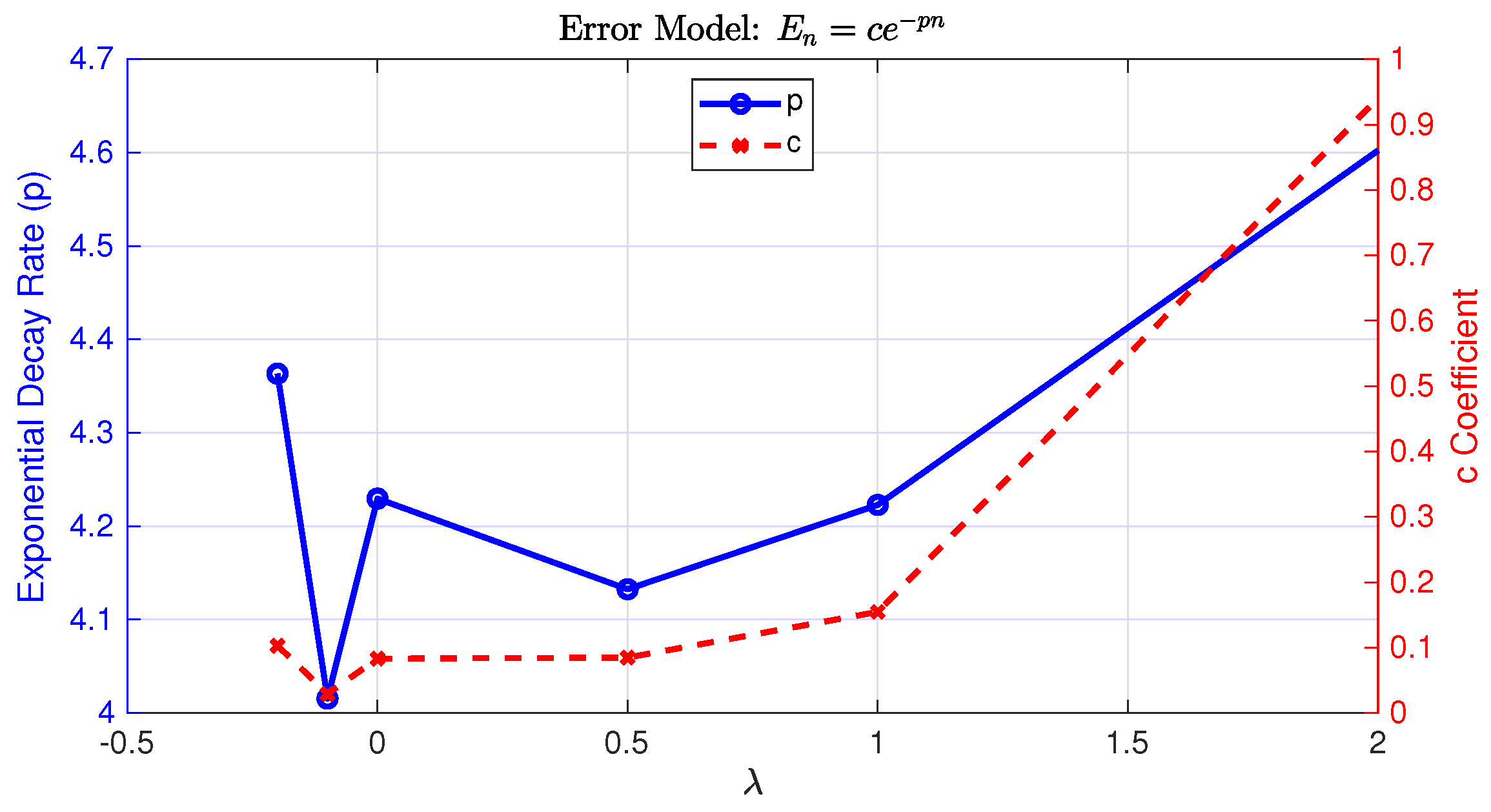
To provide empirical support for our theoretical claims on the convergence rate of the SGPS method, we analyze the error in computing the Caputo FD as a function of the number of interpolation points for various parameter values. We estimate the rate of convergence based on a semi-log regression of the error. Specifically, we assume that the error follows an exponential decay model of the form $E_n\approx c·e^{-pn}$, where p is the exponential decay rate and c is a positive constant. Taking the natural logarithm of this expression yields $ln{E}_n\approx -pn+lnc$. We can estimate p by performing a linear regression of $ln{E}_n$ against n. The magnitude of the slope of the resulting line provides an estimate for the decay rate p. As an illustration, reconsider Test Function $f_2$, previously examined in Section 2, with its error plots shown in Figure 3. Under the same data settings, Figure 5 depicts the variation in the estimated exponential decay rate (p) and coefficient (c) with respect to $\lambda$. The decay rate p remains relatively consistent across different $\lambda$ values, fluctuating slightly between 4 and 4.6, indicating that the SGPS method sustains a stable exponential convergence rate under variations in $\lambda$. The coefficient c varies smoothly between approximately 0.1 and 1, reflecting a stable baseline magnitude of the approximation error. The bounded variation in c further suggests that the method’s accuracy is largely insensitive to the choice of $\lambda$ within the considered range.

5. Case Study: Caputo Fractional TPBVP of the Bagley–Torvik Type

In this section, we consider the application of the proposed method on the following Caputo fractional TPBVP of the Bagley–Torvik type, defined as follows: 353035

$$a{}^{c}D_x^{\alpha }u+b{}^{c}D_x^{1.5}u+cu\left(x\right)=f\left(x\right),x\in {\mathsf{\Omega }}_1,$$

(35a)

with the given Dirichlet boundary conditions

$$u\left(0\right)={\gamma }_1,u\left(1\right)={\gamma }_2,$$

(35b)

where $\alpha >1,\{a,b,c,{\gamma }_{1:2}\}\subset \mathbb{R}$, and $f\in L^2\left({\mathsf{\Omega }}_1\right)$. With the derived numerical instrument for approximating Caputo FDs, determining an accurate numerical solution to the TPBVP is rather straightforward. Indeed, collocating System (35a) at the SGG set $\left\{{\widehat{x}}_{n,0:n}^{\lambda }\right\}={\widehat{\mathbb{G}}}_n^{\lambda }$ in conjunction with Equation (10) yields 363536

$$a{}^E\mathbf{Q}_n^{\alpha }{u}_{0:n}+b{}^E\mathbf{Q}_n^{1.5}{u}_{0:n}+c{u}_{0:n}=f_{0:n}.$$

(36a)

Since ${\widehat{G}}_k^{\lambda }\left(0\right)={(-1)}^k$ and ${\widehat{G}}_k^{\lambda }\left(1\right)=1\forall k\in {\mathbb{J}}_n^{+}$, according to the properties of SG polynomials, substituting the boundary conditions (35b) into Equation (1) gives the following system of equations:

$$\begin{array}{c}\left[\mathrm{trp}\left({\widehat{\lambda }}_{0:n}^{{\lambda }^{÷}}\right)\left({\left({(-1)}^{0:n}\otimes {\mathit{1}}_{n+1}\right)}^{\top }\odot {\widehat{G}}_{0:n}^{\lambda }-[{\widehat{\mathbf{x}}}_n^{\lambda }-]\right)\mathrm{diag}\left({\widehat{\varpi }}_{0:n}^{\lambda }\right)\right]u_{0:n}={\gamma }_1,\end{array}$$

(36b)

$$\begin{array}{c}\left[\mathrm{trp}\left({\widehat{\lambda }}_{0:n}^{{\lambda }^{÷}}\right){\widehat{G}}_{0:n}^{\lambda }-[{\widehat{\mathbf{x}}}_n^{\lambda }-]\mathrm{diag}\left({\widehat{\varpi }}_{0:n}^{\lambda }\right)\right]u_{0:n}={\gamma }_2.\end{array}$$

(36c)

Therefore, the linear system described by Equations (36a), (36b) and (36c) can now be compactly written in the following form:

$$\mathbf{A}{u}_{0:n}=\mathbf{F},$$

(37)

where

$$\mathbf{A}=\left[\begin{array}{c}a{}^E\mathbf{Q}_n^{\alpha }+b{}^E\mathbf{Q}_n^{1.5}+c{\mathbf{I}}_{n+1}\\ \mathrm{trp}\left({\widehat{\lambda }}_{0:n}^{{\lambda }^{÷}}\right)\left({\left({(-1)}^{0:n}\otimes {\mathit{1}}_{n+1}\right)}^{\top }\odot {\widehat{G}}_{0:n}^{\lambda }-[{\widehat{\mathbf{x}}}_n^{\lambda }-]\right)\mathrm{diag}\left({\widehat{\varpi }}_{0:n}^{\lambda }\right)\\ \mathrm{trp}\left({\widehat{\lambda }}_{0:n}^{{\lambda }^{÷}}\right){\widehat{G}}_{0:n}^{\lambda }-[{\widehat{\mathbf{x}}}_n^{\lambda }-]\mathrm{diag}\left({\widehat{\varpi }}_{0:n}^{\lambda }\right)\end{array}\right],$$

is the collocation matrix, and

$$\mathit{F}={[f_{0:n}^{\top },{\gamma }_{1:2}]}^{\top }.$$

The solution to the linear system (37) provides the approximate solution values at the SGG points. The solution values at any non-collocated point in ${\mathsf{\Omega }}_1$ can further be estimated with excellent accuracy via the interpolation Formula (1).

When $\alpha \in {\mathbb{Z}}^{+}$, Caputo FD reduces to the classical integer-order derivative of the same order. In this case, we can use the first-order GDM in barycentric form, ${\mathbf{D}}^{\left(1\right)}$, of Elgindy and Dahy [31]. This matrix enables the approximation of the function’s derivative at the GG nodes using the function values at those nodes by employing matrix–vector multiplication. The entries of the differentiation matrix are computed based on the barycentric weights and GG nodes. The associated differentiation formula exhibits high accuracy, often exhibiting exponential convergence for smooth functions. This rapid convergence is a hallmark of PS methods and makes the GDM highly accurate for approximating derivatives. Furthermore, the utilization of barycentric forms improves the numerical stability of the differentiation matrix and leads to efficient computations. Using the properties of PS differentiation matrices, higher-order differentiation matrices can be readily generated through successive multiplication by the first-order GDM:

$${\mathbf{D}}^{\left(k\right)}={\mathbf{D}}_{\left(k\right)}^{\left(1\right)},\forall k>1.$$

The SGDM of any order $k,{\widehat{\mathbf{D}}}^{\left(k\right)}$, based on the SGG point set ${\widehat{\mathbb{G}}}_n^{\lambda }$, can be generated directly from ${\mathbf{D}}^{\left(1\right)}$ using the following formula:

$${\widehat{\mathbf{D}}}^{\left(k\right)}=2^k{\mathbf{D}}_{\left(k\right)}^{\left(1\right)},\forall k\ge 1.$$

Figure 6 outlines the complete solution workflow for applying the SGPS method to Bagley–Torvik TPBVPs. The process begins with constructing the FSGIMs and, when necessary, the SGDM for integer orders. These are used to discretize the governing fractional differential equations via collocation at SGG nodes. The resulting system is assembled into a linear algebraic system, which is solved to obtain the numerical solution at collocation points. Finally, the global numerical solution is recovered by interpolating these discrete values using the SGPS interpolant.

6. Numerical Examples

In this section, we present numerical experiments conducted on a personal laptop equipped with an AMD Ryzen 7 4800H processor (2.9 GHz, 8 cores/16 threads) and 16GB of RAM, and running Windows 11. All simulations were performed using MATLAB R2023b. The accuracy of the computed solutions was assessed using absolute errors and maximum absolute errors, which provide quantitative measures of the pointwise and worst-case discrepancies between the exact and numerical solutions, respectively.

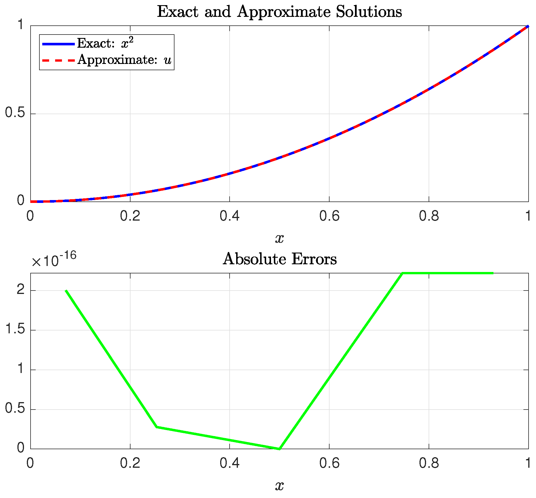
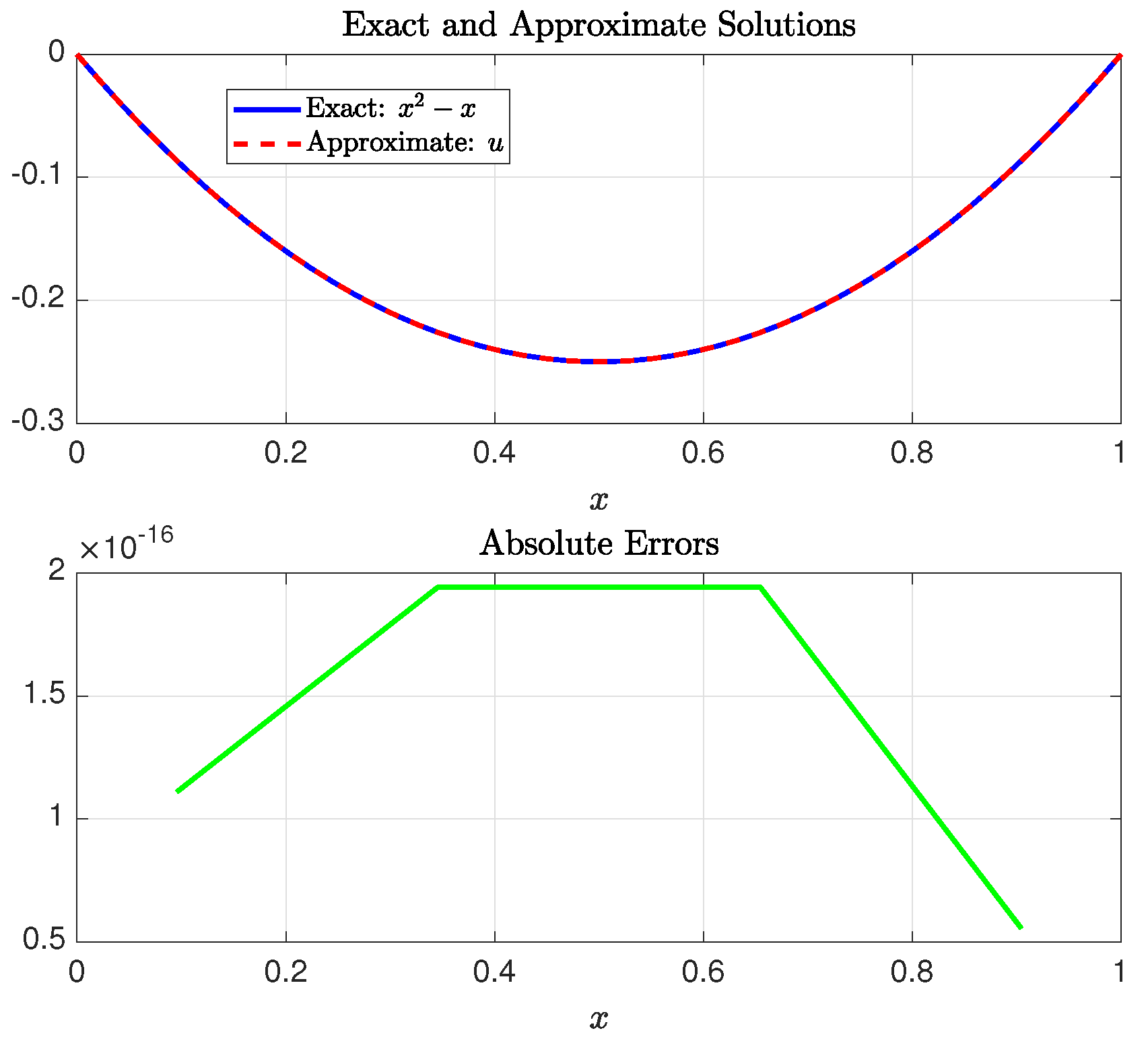
Example 1.

Consider the Caputo fractional TPBVP of the Bagley–Torvik type

$${}^{c}D_x^{2}u+{}^{c}D_x^{1.5}u+u\left(x\right)=x^2+2+4\sqrt{{\displaystyle \frac{x}{\pi }}},x\in {\mathsf{\Omega }}_1,$$

with the given Dirichlet boundary conditions

$$u\left(0\right)=0,u\left(1\right)=1.$$

The exact solution is $u\left(x\right)=x^2$. This problem was solved by Al-Mdallal et al. [32] using a method that combines conjugating collocation, spline analysis, and the shooting technique. Their reported error norm was $3.78\times {10}^{-12}$; cf. [33]. Later, Batool et al. [33] addressed the same problem using integral operational matrices based on Chelyshkov polynomials, transforming the problem into solvable Sylvester-type equations. They reported an error norm of $2.3388\times {10}^{-25}$, obtained using approximate solution terms with significantly more than 16 digits of precision. Specifically, the three terms used to derive this error included 32, 47, and 47 digits after the decimal point, indicating that the method utilizes extended or arbitrary-precision arithmetic, rather than being constrained to standard double precision. For a more fair comparison, since all components of our computational algorithm adhere to double-precision representations and computations, we recalculated their approximate solution using Equation (92) of [33] on the MATLAB platform with double-precision arithmetic. Our results indicate that the maximum absolute error in their approximate solution, evaluated at 50 equally spaced points in ${\mathsf{\Omega }}_1$, was approximately $2.22\times {10}^{-16}$. The SGPS method produced this same result using the parameters $n=n_q=4$ and $\lambda ={\lambda }_q=1.1$. The elapsed time required to run the SGPS method was $0.004732$ s. Figure 7 illustrates the exact solution, the approximate solution obtained using the SGPS method, and the absolute errors at the SGG collocation points.

Example 2.

Consider the Caputo fractional TPBVP of the Bagley–Torvik type

$${}^{c}D_x^{2}u+{}^{c}D_x^{1.5}u+u\left(x\right)=1+x,x\in {\mathsf{\Omega }}_1,$$

with the given Dirichlet boundary conditions

$$u\left(0\right)=1,u\left(1\right)=2.$$

The exact solution is $u\left(x\right)=1+x$. Yüzbaşı [34] solved this problem using a numerical technique based on collocation points, matrix operations, and a generalized form of Bessel functions of the first kind. The maximum absolute error reported in [34] (at $M=6$) was $4.6047\times {10}^{-8}$. Our SGPS method produced near-exact solution values within a maximum absolute error of $4.44\times {10}^{-16}$ using $n=n_q=\lambda ={\lambda }_q=2$; cf. Figure 8. The elapsed time required to run the SGPS method was $0.004142$ s.

Example 3.

Consider the Caputo fractional TPBVP of the Bagley–Torvik type

$${}^{c}D_x^{1.5}u+u\left(x\right)={\displaystyle \frac{2}{\mathsf{\Gamma }(3/2)}}\sqrt{x}+x(x-1),x\in {\mathsf{\Omega }}_1,$$

with the given Dirichlet boundary conditions

$$u\left(0\right)=u\left(1\right)=0.$$

The exact solution is $u\left(x\right)=x^2-x$. Our SGPS method produced near-exact solution values within a maximum absolute error of $1.94\times {10}^{-16}$ using $n=n_q=3$ and $\lambda ={\lambda }_q=1$; cf. Figure 9. The elapsed time required to run the SGPS method was $0.004160$ s.

7. Sensitivity Analysis of SG Parameters ${\forall }_{rs}n$ and $n_q$

Optimizing the performance of the SGPS method requires a thorough understanding of how the Gegenbauer parameters $\lambda$ and ${\lambda }_q$ influence numerical stability and accuracy. These parameters govern the clustering of collocation and quadrature points, directly affecting the condition number of the collocation matrix $\mathbf{A}$ and the overall robustness of the method. In this section, we present a sensitivity analysis to quantify the impact of varying $\lambda$ and ${\lambda }_q$ on the stability of the SGPS method, as measured by the condition number $\kappa \left(\mathbf{A}\right)$. The analysis specifically examines the behavior of the method when solving the Caputo Fractional TPBVP of the Bagley–Torvik Type with smaller interpolation and quadrature mesh sizes. The numerical examples from Section 6 serve as the basis for this analysis, and the results are visualized using surface plots, contour plots, and semilogarithmic plots to illustrate the condition number’s behavior across the parameter space.

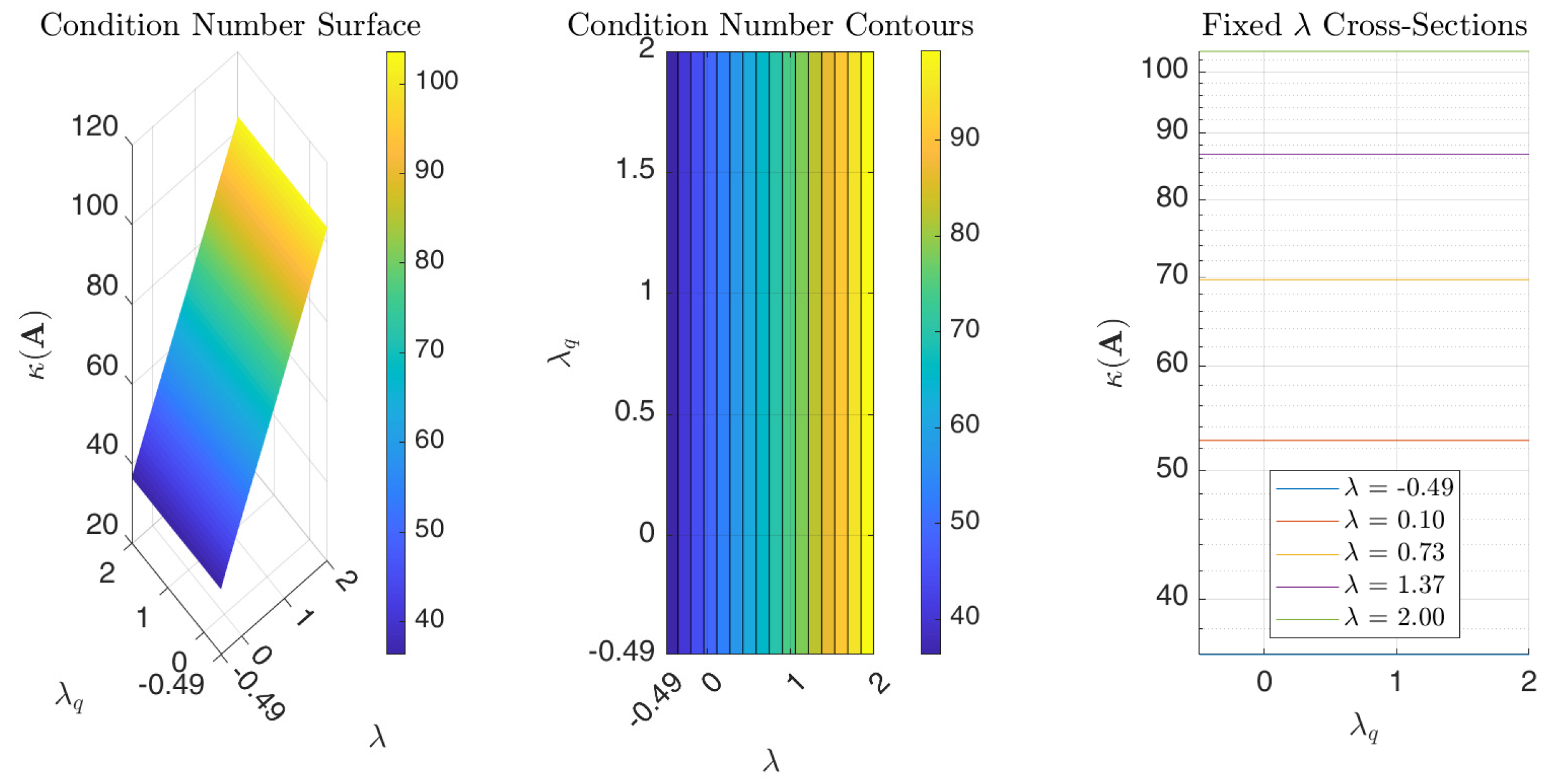
Figure 10 illustrates the influence of varying the parameters $\lambda$ and ${\lambda }_q$ on the condition number of collocation matrix $\mathbf{A}$ associated with Example 1. Higher condition numbers indicate increased sensitivity to perturbations in the input data, potentially leading to instability in the numerical solution. The results show that ${\forall }_{rs}n$ and $n_q$, the condition number is influenced by $\lambda$; as $\lambda$ increases, the condition number tends to grow linearly. Conversely, the condition number exhibits minimal sensitivity to changes in ${\lambda }_q$ within the range specified by the “Rule of Thumb.” This suggests that the stability of the method for low-degree SG interpolants and small quadrature mesh sizes is primarily dependent on the appropriate selection of $\lambda$. Specifically, choosing a $\lambda$ that is relatively large and positive can compromise stability. Conversely, the figure indicates that $\lambda$ values closer to $-1/2$ (while maintaining a sufficient distance to prevent excessive growth in SG polynomial values), combined with ${\lambda }_q$ values within the interval ${\mathcal{T}}_{c,r}$, particularly near its endpoints, yield lower condition numbers. We notice, however, that $\kappa \left(\mathbf{A}\right)$ remains in the order of ${10}^2$ for $-0.49\le \lambda ,{\lambda }_q\le 1.9$, indicating that the SGPS method is numerically stable for this range of parameters. Moreover, for double-precision arithmetic, this observation implies a potential loss of two significant digits in the worst case. However, the actual error observed in the numerical experiments is much smaller, indicating that the method is highly accurate in practice. Figure 11 and Figure 12 present further sensitivity analyses of the SGPS method’s numerical stability for Examples 2 and 3. The condition number in both examples is in the order of 10 for the parameter range considered (up to nearly 2), indicating high numerical stability for that parameter range. These figures consistently indicate that stability is influenced by $\lambda {\forall }_{rs}n$ and $n_q$, but minimally impacted by ${\lambda }_q$.

The sensitivity analysis conducted in this section reveals an important decoupling in parameter effects: while $\lambda$ primarily governs the numerical stability through its linear relationship with the condition number of the collocation matrix, ${\lambda }_q$ predominantly controls the accuracy of Caputo FD approximations, as seen earlier in Figure 2 and Figure 3, without significantly affecting system conditioning. This decoupling allows for the independent optimization of stability and accuracy. In particular, we can select $\lambda$ to ensure well-conditioned systems while tuning ${\lambda }_q$ to achieve the desired precision in derivative computations. The recommended parameter ranges ($\lambda ,{\lambda }_q\in {\mathcal{T}}_{c,r}$) provide a practical balance. Negative values of $\lambda$ and ${\lambda }_q$ close to $-0.49$ can improve stability and accuracy when using smaller interpolation and quadrature grids, while excellent quadrature accuracy is often achieved at ${\lambda }_q=0.5$. This separation of concerns simplifies parameter selection and enables robust implementations across diverse problem configurations.

8. Conclusions and Discussion

This study pioneers a unified SGPS framework that seamlessly integrates interpolation and integration for approximating higher-order Caputo FDs and solving TPBVPs of the Bagley–Torvik type, offering significant advancements in numerical methods for fractional differential equations through the following: (i) The development of FSGIMs that accurately and efficiently approximate Caputo FDs at any random set of points using SG quadratures generalizes traditional PS differentiation matrices to the fractional-order setting, which we consider a significant theoretical advancement. (ii) The use of FSGIMs allows for pre-computation and storage, significantly accelerating the execution of the SGPS method. (iii) The method applies an innovative change of variables that transforms the Caputo FD into a scaled integral of an integer-order derivative. This transformation simplifies computations, facilitates error analysis, and mitigates singularities in the Caputo FD near zero, which improves both stability and accuracy. (iv) The method can produce approximations withing near-full machine precision at an exponential rate using relatively coarse mesh grids. (v) The method generally improves numerical stability and attempts to avoid issues related to ill conditioning in classical PS differentiation matrices by using SG quadratures in barycentric form. (vi) The proposed methodology can be extended to multidimensional fractional problems, making it a strong candidate for future research in high-dimensional fractional differential equations. (vii) Unlike traditional methods that treat interpolation and integration separately, the current method unifies these operations into a cohesive framework using SG polynomials. Numerical experiments validated the superior accuracy of the proposed method over existing techniques, achieving near-machine precision results in many cases. The current study also highlighted critical guidelines for selecting the parameters $\lambda$ and ${\lambda }_q$ to optimize the performance of the SGPS method ${\forall }_{rs}\alpha$. In particular, for large interpolation and quadrature mesh sizes, and for high-precision computations, $\lambda$ should be selected within the range ${\mathsf{\Omega }}_2$, while ${\lambda }_q$ should be adjusted to satisfy $-1/2+\epsilon \le {\lambda }_q\le 2$. This ensures a balance between convergence speed and numerical stability. For general-purpose computations, setting $\lambda ={\lambda }_q=0$ (corresponding to the SC interpolant and quadrature) is recommended, as it provides optimal $L^{\infty }$-norm accuracy for smooth functions. The analysis also revealed that increasing $\lambda$ accelerates theoretical convergence but may introduce numerical instability due to extrapolation effects, while larger ${\lambda }_q$ values can slow convergence. ${\forall }_{rs}n$ and $n_q$, the sensitivity analysis in this study reveals that the conditioning of the linear system of equations produced by the SGPS method when treating a Caputo Fractional TPBVP of the Bagley–Torvik Type increases approximately linearly with $\lambda$. This indicates that smaller values of $\lambda$ in this case can lead to improved numerical stability. In particular, it is advisable to choose negative $\lambda$ values, especially in the neighborhood of $-0.49$, as evidenced by the numerical simulations, but not too close to $-1/2$, to avoid the rapid growth of SG polynomials. The conditioning of the linear system is less sensitive to variations in ${\lambda }_q$ compared to $\lambda {\forall }_{rs}n$ and $n_q$, with minimal effect on stability. However, to maintain accuracy, it is still recommended to keep ${\lambda }_q$ within the recommended interval ${\mathcal{T}}_{c,r}$, with excellent quadrature accuracy often attained at ${\lambda }_q=0.5$. These insights ensure robust and efficient implementations of the SGPS method across diverse problem settings. The SGPS method’s computational efficiency is further underscored by its predictable runtime and storage costs, as summarized in

Table 2. Computational costs and typical parameters for the SGPS method.

Aspect	Cost/Parameter	Typical Values
Runtime	Construction of FSGIM: $\mathcal{O}\left(Mn{n}_q\right)$	Small:$n,n_q=2,3,4$; $M=n$
	Application of FSGIM: $\mathcal{O}\left(Mn\right)$	Large:$n,n_q\ge 10$; $M=n$
Storage	FSGIM: $\mathcal{O}\left(Mn\right)$	Same as above
Parameter Ranges	Small n, $n_q$: $\lambda ,{\lambda }_q\in [-1/2+\epsilon ,2]$	Suggested:$\lambda \approx -0.49$, ${\lambda }_q=0.5$
	Large n, $n_q$: $\lambda \in {\mathsf{\Omega }}_2,{\lambda }_q\in [-\frac{1}{2}+\epsilon ,2]$	Suggested:$\lambda ={\lambda }_q=0$

. For practitioners, these estimates provide clear guidelines for resource allocation. The table also highlights recommended parameter ranges to balance accuracy and stability.

The current work assumes sufficient smoothness of the solution to achieve exponential convergence. For fractional problems involving weakly singular or non-smooth solutions, where derivatives may be unbounded, future research may investigate adaptive techniques—such as graded meshes or hybrid spectral–finite element approaches—to extend the method’s applicability. The robust approximation of Caputo derivatives achieved by the SGPS method creates opportunities for modeling viscoelasticity in smart materials, anomalous transport in heterogeneous media, and non-local dynamics in control theory. Future directions could include adaptive parameter tuning to capture singularities in viscoelastic models or coupling the method with machine learning to optimize fractional-order controllers. These applications would improve the method’s interdisciplinary relevance while preserving its mathematical rigor. Additionally, the SGPS approach could be extended to multidimensional fractional problems, where tensor products of one-dimensional FSGIMs can be employed. The inherent parallelizability of FSGIM matrix–vector operations makes the method particularly suitable for GPU acceleration or distributed computing. For time-dependent fractional PDEs, like fractional diffusion equations, the SGPS method can employ the FSGIM for spatial discretization, transforming the problem into a system of ODEs in time. Standard time-stepping schemes, such as Runge–Kutta or fractional linear multistep methods, can then be applied. The precomputation and reuse of the FSGIM for spatial discretization at each time step can yield significant efficiency gains in time-marching schemes.