Robust Photovoltaic Power Forecasting Model Under Complex Meteorological Conditions

Abstract

The rapid expansion of global photovoltaic (PV) capacity has imposed higher demands on forecast accuracy and timeliness in power dispatching. However, traditional PV power forecasting models designed for distributed PV power stations often struggle with accuracy due to unpredictable meteorological variations, data noise, non-stationary signals, and human-induced data collection errors. To effectively mitigate these limitations, this work proposes a dual-stage feature extraction method based on Variational Mode Decomposition (VMD) and Principal Component Analysis (PCA), enhancing multi-scale modeling and noise reduction capabilities. Additionally, the Whale Optimization Algorithm is adopted to efficiently optimize the hyperparameters of iTransformer for the framework, improving parameter adaptability and convergence efficiency. Based on VMD-PCA refined feature extraction, the iTransformer is then employed to perform continuous active power prediction across time steps, leveraging its strength in modeling long-range temporal dependencies under complex meteorological conditions. Experimental results demonstrate that the proposed model exhibits superior robustness across multiple evaluation metrics, including coefficient of determination, mean square error, mean absolute error, and root mean square error, with comparatively low latency. This research provides valuable model support for reliable PV system dispatch and its application in smart grids.

1. Introduction

With the global push towards carbon neutrality, photovoltaic (PV) power generation has become one of the fastest-growing renewable energy technologies [1,2]. According to the International Energy Agency report “Electricity 2024”, global projections for electricity demand, supply, and carbon dioxide emissions indicate that PV power generation will play a crucial role in the future. By 2030, the global renewable energy capacity is expected to grow by 2.7 times, with solar PV expected to account for 80% of this increase. However, the intermittency and volatility of PV power generation pose significant challenges to grid stability, particularly in scenarios involving rapid cloud movement or localized weather changes, where power fluctuations can exceed 70% of the rated capacity [3]. Therefore, developing high-precision PV power forecasting models has become a critical technological requirement to ensure the safe and economical operations of power systems [4].

For distributed PV power forecasting, data quality is one of the key factors affecting prediction accuracy. However, the core challenges in existing studies arise from the multi-source heterogeneity and quality defects of distributed PV power station data, shown as follows:

• Temporal and spatial mismatches between meteorological data and electrical parameters. The output of PV power is influenced by meteorological factors such as solar irradiance, temperature, and wind speed. Official meteorological stations typically provide regional macro data (with a resolution of approximately 10–20 km), while the micro-meteorological environment of the PV panel surface (irradiance, temperature, etc.) is significantly affected by local cloud cover and array layout. Due to the temporal and spatial mismatch of the data, meteorological data often cannot accurately reflect the actual irradiance on the PV panels, leading to significant prediction errors in the models [5,6];
• Defects exist in data collection systems. Approximately 38% of small- and medium-sized PV power plants still use manual meter reading to record parameters such as voltage and current, leading to random errors of 10–15% in the data. Furthermore, aging sensors and insufficient maintenance in PV plants may lead to inaccurate data collection, further impacting the performance of prediction models [7,8];
• Feature distortion occurs under extreme weather conditions. Extreme weather events, especially cloud cover and storms, can have a significant impact on the power generation of PV plants. Under conditions of high cloud coverage, the actual irradiance received by PV panels may significantly deviate from meteorological station data, resulting in a 30% or more decline in the accuracy of traditional prediction models [9,10,11]. Additionally, local weather changes such as sudden temperature rises and precipitation can directly affect the output of PV power, leading to a degradation in prediction performance during extreme weather events [12,13].

In summary, there is a direct relationship between the accuracy of PV power forecasting and data quality. In the presence of missing data, inconsistencies, noise interference, and outliers, the accuracy of PV power forecasts is often difficult to ensure. In particular, PV power forecasting in distributed PV power stations is frequently challenged by the phenomenon of Concept Drift, which arises due to various factors such as seasonal transitions, weather variability, cloud cover, sensor malfunctions, and missing data caused by human error [14]. This phenomenon leads to non-stationary changes in the statistical properties of the input features (e.g., solar irradiance, ambient temperature), thereby altering the mapping relationship between input variables and the target output (i.e., active PV power generation) over time. Therefore, how to enhance the robustness of forecasting models while ensuring data quality, particularly under complex meteorological conditions, has become a core issue in current PV power forecasting research.

PV power forecasting is a time series forecasting problem, and related studies have evolved through multiple stages, from initial statistical models to current deep learning models, with continuous development and improvement of research methods [15]. However, traditional methods and current deep learning approaches still face many challenges when dealing with complex meteorological data and fluctuating PV power outputs.

Early PV power forecasting methods primarily employed statistical models and classical machine learning methods, such as Autoregressive Integrated Moving Average (ARIMA) [16], Autoregressive Moving Average (ARMA) [17], and Support Vector Machines (SVM) [18]. Statistical models can handle seasonal and trend variations in stationary data through differencing and modeling of historical data, but their forecasting performance is poor when applied to complex PV power data [19]. ARIMA processes non-stationary sequences through differencing but struggles to capture power step changes caused by sudden irradiance fluctuations. Also, it is assumed that the input data are stationary, whereas PV power is influenced by various meteorological factors, resulting in non-stationary data with significant noise and sudden changes [20]. Consequently, the prediction accuracy of ARIMA significantly decreases when dealing with power fluctuations caused by rapid changes in solar irradiance. SVM, a common machine learning method, has been widely applied in PV power forecasting. It handles nonlinear problems using kernel functions and has strong fitting capabilities [18,21]. However, when the input feature dimensions are too high, the computational complexity of SVM increases sharply, and the prediction error grows exponentially in high-dimensional data. Additionally, Random Forest, an ensemble learning method, can handle high-dimensional data [22]. Nevertheless, due to its bagging mechanism, it easily disrupts the continuity of time series data, making it ineffective in capturing the temporal dependencies in PV power data during time series forecasting.

The above-mentioned traditional methods generally suffer from two issues: (1) they overly rely on manual feature engineering, making it difficult to fully extract the multi-scale features of PV data [23]; and (2) hyperparameter tuning relies on manual experience, lacking systematic optimization methods. As a result, the traditional methods often yield unsatisfactory performance in practical applications [24].

In addition to the evolution of statistical and machine learning models, existing engineering methods for PV power forecasting can be broadly categorized into four major types: (1) physical model-based methods, which rely on radiation transmission, thermodynamic balance, and PV system characteristics [15,20]; (2) statistical and empirical models, which establish empirical relationships between meteorological inputs and power output [16,17,19]; (3) hybrid data-driven methods, which combine signal decomposition, optimization, and prediction modules (e.g., genetic algorithms); and (4) deep learning models, which automatically learn complex spatiotemporal features.

Physical models offer high interpretability and are effective when real-time irradiance and panel configuration data are available, but they require precise system parameters and are difficult to apply to distributed PV stations with missing or erroneous data. Statistical models perform well under high-quality time-series data but fail to generalize when facing abrupt weather changes or sensor failures. Hybrid methods attempt to improve robustness via signal preprocessing and optimization algorithms but introduce parameter complexity and often lack adaptability. In contrast, deep learning models, particularly those based on Transformers architectures, offer flexibility in dealing with non-stationary, heterogeneous input features [15]. Given the challenges in our dataset—including spatially mismatched meteorological data, sensor degradation, and high noise levels—this study adopts a hybrid deep learning strategy tailored to handle low-quality; multi-source data from distributed PV stations.

With the development of deep learning technology, research on PV power forecasting has gradually shifted towards deep learning models [15], particularly Long Short-Term Memory (LSTM) networks [25,26] and Transformer models [27,28]. LSTM networks capture long-term dependencies in time series data through gating mechanisms and can alleviate the vanishing gradient problem found in traditional Recurrent Neural Networks to some extent [29]. However, LSTMs still face the issues of vanishing and exploding gradients when handling long time sequences. Additionally, LSTM performance is influenced by the training data, especially in long-term forecasting, where the Mean Squared Error (MSE) significantly increases, leading to unstable predictions. Transformers, with their self-attention mechanism, excel at capturing global feature information and have shown great potential in PV power forecasting. Transformers can accelerate model training through parallel computation and maintain high prediction accuracy over long time series. However, traditional Transformers suffer from distortion in position encoding when handling long sequences, leading to inaccurate capturing of temporal information, which in turn affects the model’s prediction accuracy. To improve performance, variants such as DLinear and PatchTST have been proposed. DLinear adopts a decomposition strategy that separates trend and seasonal components, enabling better generalization in time-series prediction [30,31]. PatchTST, on the other hand, introduces a patching and tokenization scheme that significantly enhances long-sequence modeling ability through Transformer blocks [31,32]. Thus, current improvements in prediction scenarios mainly focus on two directions: (1) designing hybrid architecture models such as the Convolutional Neural Network and Long Short-Term Memory (CNN-LSTM) combined model, which extracts spatial features through convolutional layers and captures temporal information using LSTM [27,33]. However, this approach does not fully solve the forecasting delay problem under sudden weather changes; and (2) optimizing the attention mechanism, such as the Informer model, which reduces computational complexity through the ProbSparse attention mechanism [34], but sacrifices responsiveness to abnormal fluctuations.

In order to overcome the limitations of single models, multi-module integration methods have gradually become a research hotspot. Variational Mode Decomposition (VMD) is a signal decomposition method that adapts to signals by solving a constrained variational problem, decomposing complex signals into multiple intrinsic frequency modes [28]. This allows for the extraction of multi-scale features, making VMD particularly suitable for processing non-stationary and noisy signals. Compared with traditional Empirical Mode Decomposition, VMD has stronger noise resistance and can effectively avoid the problem of mode mixing [35].

Principal Component Analysis (PCA), as a classic dimensionality reduction tool, can effectively mitigate multicollinearity among features [36]. When applied to the components obtained from VMD, PCA helps to reduce the dimensionality of the data by projecting it onto a smaller number of orthogonal components that capture the majority of the variance [37]. By combining VMD and PCA, the main features of PV power data can be effectively extracted and reduced in dimensionality, thereby reducing computational complexity. Although VMD and PCA excel in signal decomposition and dimensionality reduction, they have limitations in capturing the inherent nonlinear features of PV data. To address this issue, intelligent optimization algorithms, such as the Whale Optimization Algorithm (WOA), have been widely used to optimize model hyperparameters, particularly for models with nonlinear architectures [38,39]. WOA, by mimicking the hunting behavior of whales, effectively avoids local optima and accelerates the model’s convergence speed, which is particularly important for handling high-dimensional nonlinear problems [40]. Nevertheless, existing multi-module integration methods still face challenges in parameter optimization, handling nonlinear features, and integrating optimization algorithms with deep learning models, which require further improvements. In this context, the iTransformer model, based on the Transformer architecture, demonstrates exceptional nonlinear modeling capabilities, effectively capturing complex dependencies in time-series data [41]. Therefore, combining WOA for hyperparameter optimization with iTransformer for nonlinear modeling significantly improves the accuracy of PV power forecasting.

Unlike most studies where meteorological and operational data are reliable and directly accessible, the forecasting environment in this work is more complex and unstable. Traditional research is usually conducted in contexts where data are complete and meteorological data are readily available, whereas in the actual situation of this work, factors such as missing data, transcription errors, and cloud cover significantly impact the prediction results. Therefore, the main challenge of this work lies in maintaining the robustness of PV power forecasting in a complex environment, especially in the presence of uncertainties such as data missing, transcription errors, and external obstructions, which ensures the stability and accuracy of the model under such interference.

To this end, this work proposes an integrated PV power forecasting model based on VMD-PCA-WOA-iTransformer, aiming to address the robust prediction of PV power under complex meteorological conditions. PV power generation is influenced by various meteorological factors, such as cloud cover variations and temperature fluctuations, leading to significant fluctuations in its power output. Traditional forecasting methods often perform poorly under such conditions. To tackle these challenges, this work introduces an innovative PV power forecasting framework by integrating multiple modules, combining signal decomposition techniques, deep learning models, and optimization algorithms. In particular, VMD decomposes the original PV power signal into several intrinsic mode functions by solving a constrained variational optimization problem. The key parameter in VMD, the number of decomposition modes K, directly affects the resolution of extracted frequency components. In this work, K is determined empirically based on the spectral entropy of the PV signal to ensure an optimal balance between over- and under-decomposition. PCA then reduces dimensionality while retaining 95% of the variance, thus improving computational efficiency. WOA, simulating the bubble-net foraging behavior of humpback whales, is adopted to tune hyperparameters of the iTransformer by balancing global exploration and local exploitation. This significantly improves the model’s convergence and avoids getting trapped in local optima. The innovations of this work are summarized as follows:

• Dual-Stage Feature Selection Mechanism: The dual-stage feature selection mechanism proposed in this work combines VMD and PCA. First, VMD is used for multi-scale signal decomposition to extract effective temporal features and avoid mode mixing issues. Then, PCA is used for dimensionality reduction, and a nonlinear weighting method is incorporated to enhance the model’s ability to express nonlinear features, further improving the prediction accuracy of the model;
• WOA-Based Hyperparameter Optimization: This work introduces WOA for hyperparameter optimization of iTransformer. It conducts a global search and fine-tuning for key hyperparameters in the iTransformer model (including learning rate, the number of attention heads, and hidden layer dimensions), enhancing the model’s prediction accuracy and adaptability;
• Robust Prediction of the Integrated Model: The integrated model proposed in this work can remain stable and provide reliable prediction results even when data are incomplete, missing, or affected by external obstructions (such as cloud cover). Furthermore, integrating WOA, iTransformer, VMD, and PCA not only enhances the model’s ability to handle nonlinear features but also provides a comprehensive solution, from feature extraction and dimensionality reduction to model optimization.

The rest of the paper is organized as follows: The next section presents the data processing method of the nonlinear data sets. Then, Section 3 illustrates the prediction method of the integrated model. Section 4 designs the numerical experiments and finds the optimal parameters of the model. In Section 5, typical cases are presented to test the performance of the proposed model structure. Finally, the conclusion and future works are given in Section 6.

2. Data Processing

This paper focuses on the robust PV power forecasting of PV power plants, with data sourced from the on-site monitoring system and local meteorological station data. The data includes electrical parameters such as current, voltage, and active power, as well as environmental data, including temperature, ground radiation, direct radiation, and diffuse radiation. Due to various levels of noise and recording errors in the on-site data, as well as significant differences in sunlight duration across different time periods (for example, some data ends at 6 PM or 8 PM), these factors need to be carefully considered during data preprocessing to ensure proper time-series alignment and stability. This preprocessing step aims to update the dataset and eliminate noise and interference, ensuring clean and reliable input for subsequent feature engineering. Among the collected data, the total active power is recorded by the energy meter, and the power data are based on the total active power, which is then back-calculated to the three-phase active power.

2.1. Resampling Technique

For PV power forecasting, the total number of effective sunlight hours varies each day, which leads to inconsistencies in the data. To address this issue, we employ a resampling technique to unify the daily effective time period, ensuring that the data are consistent across days. The effective time period is set from 08:00 to 20:00 (a total of 13 h), which is the union of the effective sunlight hours across all datasets. Thus, this time period captures the majority of the daily solar radiation. This uniform time frame allows for better comparability between days, reducing potential bias in the data that could arise from varying daylight hours.

The original dataset also suffers from irregular sampling intervals. This irregularity arises because certain PV power plants do not utilize electronic or automated data collection systems. As a result, data are manually recorded, leading to human errors and inconsistencies in the sampling intervals. To overcome this limitation, we resample the data such that each point corresponds to hourly intervals, ensuring uniformity in data representation. This process involves interpolating missing data points to ensure temporal continuity, which is essential for capturing accurate temporal dynamics. Additionally, by restricting the analysis to the effective time period between 08:00 and 20:00, we mitigate the influence of low light conditions during nighttime and the early morning or late evening hours. Without doing so, the noise and unnecessary complexity would be introduced into the forecasting model.

To formalize the resampling process, let $t$ represent the original time variable ($t_{raw}\in \left[01:00,09:00,\dots ,24:00\right]$), and let $P_{raw}\left(t_{raw}\right)$ denote the raw PV power data sampled at irregular intervals. The resampled data at hourly spaced intervals t, denoted by $P_{resampled}\left(t\right)$, is obtained through an interpolation technique as follows:

$$P_{resampled}\left(t\right)=interp\left(P_{raw}\left(t_{raw}\right),t\right), t\in \left[08:\mathrm{00,09}:00,\dots ,20:00\right]$$

(1)

where $t$ represents the new, uniformly spaced time points within the interval from 08:00 to 20:00. Also, $interp\left(P_{raw}\left(t_{raw}\right),t\right)$ denotes the interpolation function that generates values for the missing data points at the new time points. This interpolation ensures that the time series is continuous and smooth throughout the day.

By comparing the resampled data to the original dataset, we observe a significant improvement in the smoothness and completeness of the time series. This resampling process lays a solid foundation for subsequent feature extraction and modeling tasks, providing a more reliable and consistent dataset for the prediction of PV active power output.

2.2. Outlier Correction

It is well known that the quality of the data directly affects the model’s performance. To ensure the reliability and accuracy of the prediction results, several outlier correction methods are proposed in this work.

2.2.1. Three-Phase Data Validation

Due to potential errors during data recording, discrepancies may arise between the three-phase active power and the total active power. To ensure consistency and reliability, we first validate the original three-phase active power ($P_A\left(t\right)$, $P_B\left(t\right)$, $P_C\left(t\right)$) and the original total active power ($P_{total}\left(t\right)$). In some cases, the sum of the three-phase powers does not match the total power and needs to be corrected based on the power factor formula. Assuming that the power factor is one and the voltage data are accurate, the relationship between the three-phase powers can be represented by the following equation.

$$P_{total}\left(t\right)=P_A\left(t\right)+P_B\left(t\right)+P_C\left(t\right), t\in \left[08:\mathrm{00,09}:00,\dots ,20:00\right]$$

(2)

If the number of decimal places of the total active power is consistent with that of the three-phase active power data, or the significant digits of the total active power are greater than those of the three-phase data, the total active power is taken as the reference to reverse calculate the average active power for each phase ($P_A^{Ave}\left(t\right),P_B^{Ave}\left(t\right),P_C^{Ave}\left(t\right)$). By averaging the original total active power, the active power for each phase is derived. Based on the physical properties of PV modules, which can be modeled as a voltage source with operating voltage fluctuating around the maximum power point, it is assumed that the voltage for each phase is maintained at the voltage corresponding to the maximum power point. This assumption allows for the reverse calculation of the current for each phase, followed by the computation of the average current for the three phases, thereby providing data support for subsequent feature design. If the data are erroneous such that Equation (2) does not hold, then we can correct the currents of the three phases based on the following equations:

$$P_A^{Ave}\left(t\right)=P_B^{Ave}\left(t\right)=P_C^{Ave}\left(t\right)={\displaystyle \frac{P_{total}\left(t\right)}{3}}$$

(3)

$$I_A^{correct}\left(t\right)={\displaystyle \frac{P_A^{Ave}\left(t\right)}{V_A\left(t\right)·cos\phi }}$$

(4)

$$I_B^{correct}\left(t\right)={\displaystyle \frac{P_B^{Ave}\left(t\right)}{V_B\left(t\right)·cos\phi }}$$

(5)

$$I_C^{correct}\left(t\right)={\displaystyle \frac{P_C^{Ave}\left(t\right)}{V_C\left(t\right)·cos\phi }}$$

(6)

where $I_A^{correct}\left(t\right)$, $I_B^{correct}\left(t\right)$, and $I_C^{correct}\left(t\right)$ are the corrected currents of phases A, B, and C, $V_A\left(t\right)$, $V_B\left(t\right)$, and $V_C\left(t\right)$ are the real operating voltages of phases A, B, and C, and $cos\phi$ is the power factor.

2.2.2. Total Active Power Correction

In the data collection and manual recording process, PV power plants with imperfect digitalization often encounter inconsistencies in active power data. Due to individual counting habits, decimal places are often omitted or rounded in the data. For example, the total active power data from 10 a.m. to 12 p.m. on 2 January 2022 are recorded as follows: integer value (198 kW), one decimal place (229.5 kW), and two decimal places (227.25 kW). Although these values correspond to three consecutive time points within the same day, their significant digits differ, which can lead to prediction accuracy deviations. When data are missing for a particular time point, the number of decimal places in the surrounding time points may not align, making traditional linear interpolation methods insufficient for accurately estimating the missing values. Data exploration reveals that the highest decimal precision retained for active power in the dataset is two decimal places. Therefore, formatting the data to retain two decimal places can reduce some of the errors. However, in practice, the data precision may exceed two decimal places, resulting in a mismatch between the total active power and the sum of the three-phase active power.

This error not only causes deviations under static conditions but is also more likely to affect accuracy under dynamic conditions, such as varying weather conditions. While the discrepancy in decimal places is small, it is numerically significant and cannot be ignored. As such, a more precise interpolation method is required to fill in the missing decimal parts. Since the error originates from uniform formatting, it manifests as a systemic error that remains relatively stable throughout the entire time series. This summation error caused by the limitation of decimal place retention is essentially a special case of linear error.

The real total active power in the dataset is denoted as $P_{total}^{real}\left(t\right)$, which differs from the true value due to decimal point limitations and needs to be corrected. The corrected total active power is represented as $P_{total}^{corrected}\left(t\right)$. The voltage and current data in the dataset are retained to two decimal places, and the formatted total active power is expressed as follows.

$$P_{total}^{rounded}(t)=round(P_A\left(t\right)+P_B\left(t\right)+P_C\left(t\right),2)$$

(7)

The resulting error can be expressed using the following formula.

$$ϵ\left(t\right)=P_{total}^{real}\left(t\right)-P_{total}^{rounded}(t)$$

(8)

To eliminate this error, the correction function is proposed as follows.

$$P_{total}^{correct}\left(t\right)=P_{total}^{rounded}\left(t\right)+f\left(ϵ\left(t\right)\right)$$

(9)

where $f\left(ϵ\left(t\right)\right)$ is the correction function based on the error $ϵ\left(t\right)$, which can be obtained through data fitting.

2.2.3. Meteorological Data Deviation

(1)

Cloud Cover

At certain times, changes in cloud cover may result in actual received irradiance being lower than the solar radiation data provided by meteorological stations, leading to a sudden drop in the power output. In this case, the actual irradiance $I_{actual}$ can be corrected using the following formula.

$$I_{actual}=I_{forecast}·{\alpha }_c$$

(10)

where $I_{forecast}$ is the irradiance predicted by the meteorological station, and ${\alpha }_c$ is the correction factor representing the impact of cloud cover.

(2)

Equipment Failure or Maintenance

In some instances, PV system equipment may be offline or under maintenance, resulting in actual power output being lower than the theoretical value. In such cases, a correction factor β is introduced to adjust the power.

$$P_{actual}=P_{forecast}·{\beta }_e$$

(11)

where ${\beta }_e$ is the correction factor based on the equipment’s health status, with values ranging from 0 to 1.

By applying these outlier correction methods, the quality of the PV power data can be improved, ensuring the reliability of the data used for model training.

2.3. Missing Value Imputation

Missing data often arises due to various factors, such as communication failures, equipment malfunctions, and human error during data collection. Two methods are presented to handle the missing data—linear interpolation and regression-based imputation—tailored to predict the total active power of PV systems.

2.3.1. Linear Interpolation Method

Linear interpolation is a widely used technique for imputing missing values in time series data, especially for data points that are missing consecutively over short periods. For this method, it is assumed that the missing values lie along a straight line between the available data points before and after the missing interval. During data collection or registration, active power, voltage, and current data at a specific moment may miss decimal places, leading to significant deviations in the prediction of active power data. To compensate for the missing values, data from the preceding and succeeding moments will be used. Missing data typically arises from the PV electrical operation data collected from the PV station monitoring platform, while the meteorological data from the official weather station is complete and does not have any missing values. To address this issue, we apply linear interpolation for correction, shown as follows.

$$V\left(t\right)=V\left(t_1\right)+{\displaystyle \frac{V\left(t_2\right)-V\left(t_1\right)}{t_2-t_1}}·\left(t-t_1\right)$$

(12)

where $V\left(t_1\right)$ and $V\left(t_2\right)$ are the known data points at times $t_1$ and $t_2$, respectively, with $t_1$ occurring before $t_2$ and $t$ is the time point for interpolation.

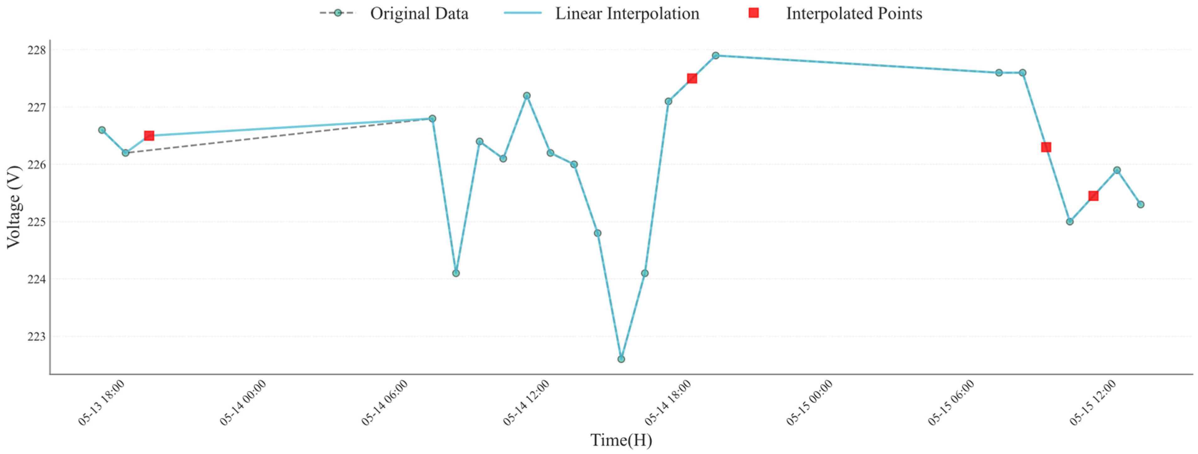
This interpolation method helps to fill in incomplete missing values, ensuring data continuity and consistency. The incomplete imputation results of multi-moment voltage values of phase A based on linear interpolation are shown in Figure 1. The dashed line represents the connection between original data points before linear interpolation, while the solid line depicts the voltage distribution curve after linear interpolation, incorporating both original and interpolated points. Green points indicate the voltage values recorded at each time point in the original dataset, whereas red squares denote the estimated voltage values at missing time points obtained through linear interpolation.

2.3.2. Regression-Based Imputation Method

Complete missing data are a commonly seen issue, often caused by sensor failures, communication disruptions, or manual error during data recording. In some cases, multiple consecutive time points may have missing data, further complicating the data recovery process. The TimesNet model is applied for imputing completely missing values. TimesNet is a deep learning architecture that is capable of handling missing values in time series data and accurately predicting them by capturing the temporal characteristics of the data [42].

For missing values in key features, such as total active power, we utilize meteorological data, including temperature, surface radiation, direct normal radiation, and diffuse radiation, to predict missing power values through regression models. Since these parameters are correlated with total active power, we hypothesize that they can effectively fill missing power data. The regression model used for imputation is shown below.

$$P_{active}={\beta }_0+{\beta }_1·T+{\beta }_2·G_h+{\beta }_3·G_d+{\beta }_4·G_s+\epsilon$$

(13)

where $P_{active}$ is the total active power; $T$ is the temperature; $G_h$ is the surface horizontal radiation; $G_d$ is the normal direct radiation; $G_s$ is the scattered radiation; ${\beta }_0$, ${\beta }_1$, ${\beta }_2$, ${\beta }_3$, and ${\beta }_4$ are the model coefficients; and $\epsilon$ is the error term.

This regression model is trained using historical meteorological data, which allows the estimation of missing power values by leveraging the relationships between the meteorological features and total active power. Also, once the model is trained, it can predict the missing active power values for any given set of meteorological data.

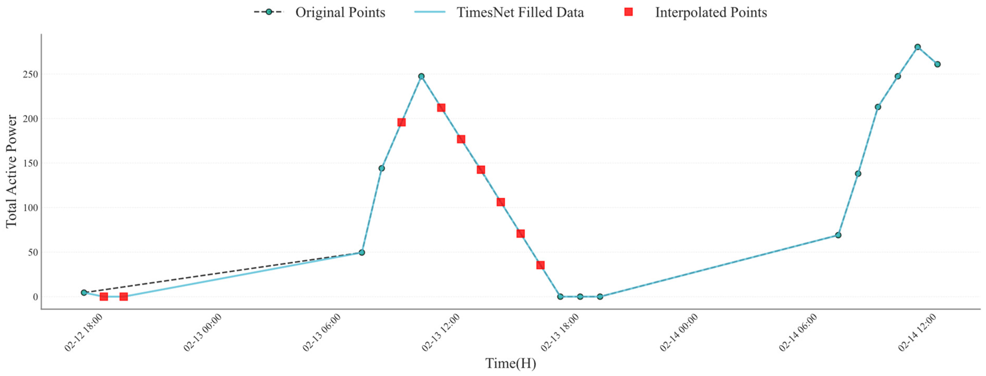
For the cases where significant gaps exist in the data, a deep learning model is adopted for missing data imputation. This model is trained to predict missing values by leveraging the temporal nature of the data. The complete imputation results of multi-moment active power based on TimesNet are shown in Figure 2. During the training process, portions of the data are masked, and the model learns to predict the masked values by minimizing the MSE loss shown as follows.

$$L_{MSE}={\displaystyle \frac{1}{N_r}}\sum _{i=1}^{N_r}{\left(y_i-{\widehat{y}}_i\right)}^2$$

(14)

where $y_i$ is the actual value of total active power, ${\widehat{y}}_i$ is the predicted value for the missing data point of total active power, and $N_r$ is the total number of data points in the process of complete imputation.

2.4. Time Series Feature Reconstruction

Due to the complexity of the data and the influence of noise, the effective extraction of temporal features plays a crucial role in enhancing the accuracy of the predictive model. To improve the model’s sensitivity to time-series features, this work integrates physical models with time-series stabilization methods by employing normalization and smoothing techniques to optimize the feature extraction capability and the training efficiency of the model.

(1)

Normalization

Time series stabilization refers to the removal of seasonal and trend-related fluctuations in the data, ensuring that the statistical properties remain constant over time. This enhances the model’s ability to learn temporal patterns effectively. Normalization is adopted for scaling the original data such that it conforms to the requirements of machine learning models, especially when the features have different magnitudes. To eliminate these differences and accelerate the convergence of the model, we use Min-Max Normalization in this work. The formula for Min-Max Normalization is given in the following equation.

$$x_{norm}={\displaystyle \frac{x-\mathit{min}\left(x\right)}{\mathit{max}\left(x\right)-\mathit{min}\left(x\right)}}$$

(15)

where $x_{norm}$ is the normalized value, $x$ is the original data, and $\mathit{min}\left(x\right)$ and $\mathit{max}\left(x\right)$ represent the minimum and maximum values of the original data $x$, respectively. This method maps all input features to the range [0, 1], eliminating magnitude differences between variables and ensuring that each feature has an equal impact on the model.

(2)

Log Transformation

Given that some input features may exhibit significantly skewed distributions (such as meteorological data or measurements of voltage and current), the log transformation is performed on these skewed data before normalization. The formula for the log transformation is

$$x_{log}=\mathit{log}\left(x+C_{log}\right)$$

(16)

where $x_{log}$ is the log-transformed data, $x$ is the original data, and $C_{log}$ is a small constant used to avoid undefined logarithmic values for zero. The log transformation brings the data closer to a normal distribution, helping to reduce extreme fluctuations and improve the model’s predictive accuracy.

(3)

Smoothing

Smoothing is another effective time-series processing method that reduces the impact of outliers and short-term fluctuations on the overall trend. In this work, a moving average approach is used for smoothing, which calculates the average of data within a fixed time window. This method can effectively reduce short-term noise and retain long-term trends. The formula for smoothing progress is given as follows.

$$x_{smoothed}\left(t\right)={\displaystyle \frac{1}{N_w}}\sum _{j=t-{\displaystyle \frac{N_w-1}{2}}}^{t+{\displaystyle \frac{N_w-1}{2}}}x\left(j\right)$$

(17)

where $x_{smoothed}\left(t\right)$ is the smoothed value at the current time $t$, $N_w$ is the size of the moving window (typically an odd number to ensure symmetry), and $x\left(j\right)$ is the data point at time point $j$ within the sliding time series. The window is symmetrical around the current time $t$, and the calculation considers all data points in the defined range from $t-{\displaystyle \frac{N_w-1}{2}}$ to $t+{\displaystyle \frac{N_w-1}{2}}$.

3. Methodology

This work proposes a method for predicting the total active power of PV systems based on meteorological data and average voltage-current features. The prediction process uses the sliding window technique, which divides the time-series data into consecutive windows, each containing 15 days of data (195 data points). Adjacent windows overlap, with a step size of one hour. Each window serves as a sample containing time information and corresponding environmental parameters (e.g., temperature, radiation, current, and voltage for each phase). Based on these window samples, the model predicts the PV power for the next 7 days. Thus, this work focuses on short-term PV power forecasting, in which historical data over 15 days is used to predict the power output for the next 7 days.

To improve prediction accuracy, this work combines VMD, PCA, and the iTransformer model. VMD is used to decompose the original signal into multiple modal components, which helps extract different frequency features and enhances the model’s ability to adapt to data diversity and complexity. PCA is then applied to reduce the dimensionality of the features, eliminating redundant information and retaining the most representative features to accelerate the model training and improve generalization. Finally, iTransformer, based on the Transformer architecture with a self-attention mechanism, is used for multi-step prediction of PV power, effectively capturing long-term dependencies in the time-series data. To optimize the hyperparameters of iTransformer, WOA is employed. WOA helps avoid local optima, thus improving the prediction accuracy of the model. Through this integrated approach, the constructed model is able to accurately predict future PV power and provide a scientific basis for the optimization and scheduling of PV power plants.

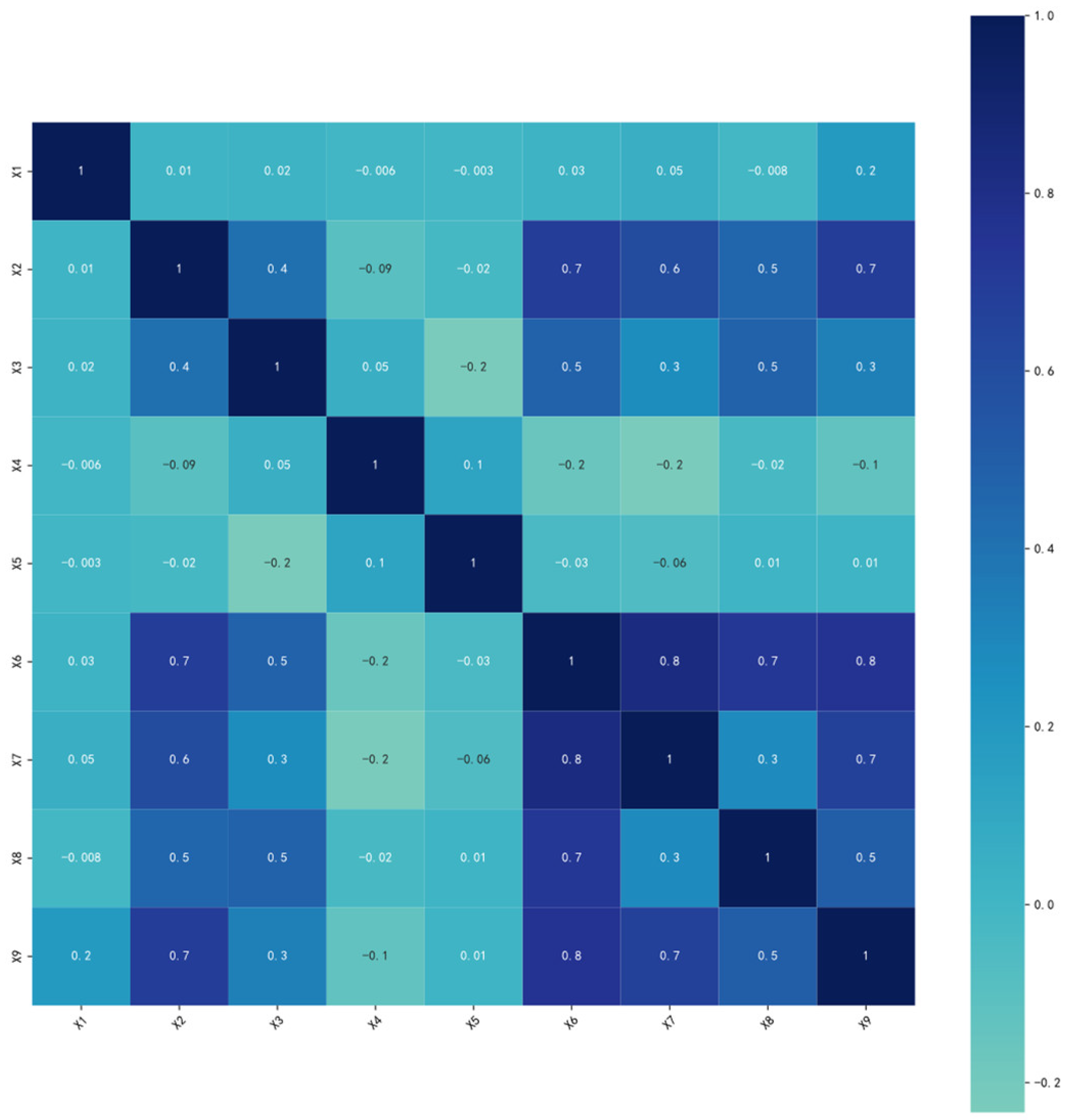
3.1. Feature Correlation Analysis

The feature correlation analysis is performed to identify the most relevant input features for predicting total active power. The correlation between different features is quantified using a correlation coefficient calculated as follows:

$$r_{xy}={\displaystyle \frac{{\sum }_{k=1}^{N_f}\left(x_k-\bar{x}\right)\left(y_k-\bar{y}\right)}{\sqrt{{\sum }_{k=1}^{N_f}{\left(x_k-\bar{x}\right)}^2{\sum }_{k=1}^{N_f}{\left(y_k-\bar{y}\right)}^2}}}$$

(18)

where $r_{xy}$ denotes the correlation coefficient between two different features, $x_k$ and $y_k$ represent the individual values of two features X and Y, respectively, $\bar{x}$ and $\bar{y}$ are their respective means over the dataset, respectively, and $N_f$ is the total number of data points in the process of feature correlation analysis.

The original feature name is shown in

Table 1. Original feature set.

Feature	Feature Name
X1	The Average Voltage at the Previous Moment
X2	The Average Current at the Previous Moment
X3	Temperature
X4	Precipitation
X5	Surface Wind Speed
X6	Surface Horizontal Radiation
X7	Normal Direct Radiation
X8	Scattered Radiation
X9	Total Active Power

. Through this correlation analysis, features that exhibit a strong correlation with the target variable (the total active power) can be identified in Figure 3. The features that are found to be significantly correlated with the total active power are retained for further feature optimization, while features with weak correlations, such as wind speed, precipitation, and reactive power, are discarded. To avoid the data leakage, we eliminate features directly related to the target variable, the total active power, from the feature set. As a result, the following features are removed from the dataset: ‘Phase A Voltage’, ‘Phase B Voltage’, ‘Phase C Voltage’, ‘Phase A Active Power’, ‘Phase B Active Power’, and ‘Phase C Active Power’. After eliminating redundant and weakly correlated features, we select the following six features to form the final feature set for model training: ‘The average voltage at the previous moment’ (X1), ‘The Average Current at the Previous Moment’ (X2), ‘Temperature’ (X3), ‘Surface Horizontal Radiation’ (X5), ‘Normal Direct Radiation’ (X6), and ‘Scattered Radiation’ (X7).

The selected features are then normalized and processed to enhance the model’s predictive performance, ensuring that they are appropriately scaled and aligned with the model requirements. This feature selection and correlation analysis ensure that only the most relevant and non-redundant features are used in the subsequent predictive modeling, minimizing the risk of overfitting and improving the model’s interpretability and accuracy.

3.2. Variational Mode Decomposition

VMD is employed to preprocess features selected through feature correlation analysis by decomposing the original signal into multiple modal components. These components capture different frequency bands or time scales within the signal, enhancing the model’s ability to learn from various signal characteristics [43]. VMD divides the original signal into high-frequency components (fast oscillations) and low-frequency components (trend changes), improving the understanding of complex time-series data. VMD is utilized in this study as a key preprocessing technique to enhance the interpretability and regularity of PV-related time-series signals. It adaptively decomposes the input signals into a predefined number of sub-signals, each of which captures a specific frequency band and is relatively independent from the others. The mathematical formulation for VMD is given by

$$\underset{\left\{u_l\right\}}{min}\sum _{l=1}^K\parallel {\displaystyle \frac{\partial }{\partial t}}\left(u_l\left(t\right)+\lambda \cdot \varphi \right){\parallel }^2+\alpha \cdot \sum _{l=1}^K\parallel f_{in}-u_l{\parallel }^2$$

(19)

where $u_l\left(t\right)$ represents the l-th mode component, $K$ is the number of modes, into which the signal is decomposed, $\lambda$ is a balancing parameter for the data fidelity constraint, $\varphi$ is the dual variable used in the optimization to enforce the smoothness of the modal components in the time domain, $f_{in}$ represents the selected feature signals through feature correlation analysis, which will be decomposed into multiple modes, and $\alpha$ is the penalty term that controls the data fidelity.

By utilizing VMD, the original PV power signal is transformed into a set of sub-signals that are more regular and easier to interpret, enhancing feature extraction and improving model learning capabilities.

For PV power prediction, meteorological data and electrical parameters (such as average voltage and current) are used as input features, alongside the modal components obtained from VMD decomposition. Each modal component represents a different frequency characteristic of the original signal and is relatively independent, yet together, they form a comprehensive representation of the signal. The integration of these model components as additional features helps the model more accurately capture the diverse patterns and behaviors presented in PV power data, thereby enhancing prediction accuracy. Mathematically, the decomposed features after VMD are formulated as follows:

$$X_{decomposed}=\left[u_1\left(t\right),u_2\left(t\right),\dots ,u_K\left(t\right)\right]$$

(20)

where $X_{decomposed}$ represents the set of decomposed modal components, K denotes the number of modes (in this case, K = 25), $u_1\left(t\right),u_2\left(t\right),\dots ,u_K\left(t\right)$ are the modal components at time $t$, where each component represents a distinct mode corresponding to different frequency characteristics of the original signal.

The selection of VMD parameters was based on extensive empirical testing and guided by established literature in Section 1 to ensure optimal decomposition performance and model stability. The VMD decomposition parameters used are summarized as follows:

• Penalty parameter ($\alpha =500$): This term controls the bandwidth of each mode. A higher $\alpha$ forces the modes, to be narrower in frequency, promoting smoother decomposition. The value is determined via grid search to ensure accurate mode separation without excessive overfitting;
• Dual ascent step ($\tau =0$): This parameter controls the update rate of the Lagrange multipliers. A zero value stabilizes the convergence of the decomposition process;
• Number of modes (K ∈ [1, 10]): The optimal value of K is determined by evaluating the trade-off between signal reconstruction accuracy and model complexity. This ensures that the signal is neither under- nor over-decomposed;
• DC component setting (DC = True): DC = True indicates that the first mode is initialized as the zero-frequency (DC) component, which helps to capture the trend part of the signal;
• Initialization (init = 0): init = 0 means all center frequencies are initialized to zero to avoid bias in decomposition;
• Tolerance (tol = $1\times {10}^{-6}$): tol = $1\times {10}^{-6}$ determines the convergence criterion of the iterative process, ensuring precise convergence while avoiding computational inefficiency.

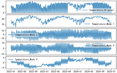
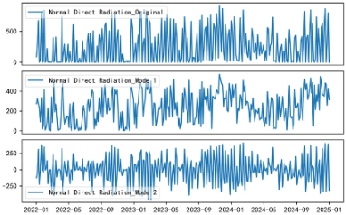
After performing VMD, the resulting decomposition of features is shown in

Table 2. The decomposition results of features based on VMD.

Original Feature	Number of Decomposed Modes	Energy Distribution Plot
The Mean of Voltage at the Previous Moment	3
The Mean of Current at the Previous Moment	9
Temperature	4
Surface Horizontal Radiation	3
Normal Direct Radiation	2
Scattered Radiation	6

.

3.3. Principal Component Analysis

Based on VMD decomposition, we further apply PCA to reduce the dimensionality of the extracted features. The purpose of PCA is not only to reduce data redundancy but also to construct a more compact and interpretable feature space that preserves most of the signal’s variance, which is critical for improving forecasting model performance. The core of PCA is to extract the most representative orthogonal feature vectors from the data by performing eigenvalue decomposition of the covariance matrix, thereby retaining the main information and removing redundant data. It can reduce the dimensionality, accelerate the model training, and improve the generalization ability. To apply PCA, the covariance matrix $Cov$ should be known, and it is obtained by the following equation.

$$Cov={\displaystyle \frac{1}{N_{cov}}}\sum _{p=1}^{N_{cov}}\left(X_p-\bar{X}\right){\left(X_p-\bar{X}\right)}^T$$

(21)

where $X_p$ is the p-th sample, $\bar{X}$ is the sample mean, and $N_{cov}$ is the number of samples. Then, eigenvalue decomposition of the covariance matrix is performed to obtain the eigenvalue matrix $A_e$ and eigenvector matrix $V_e$, which satisfy the relation:

$$Cov\times V_e=V_e\times A_e$$

(22)

PCA is applied to the feature matrix formed by the modal components after VMD, which typically exhibits multicollinearity and high dimensionality. PCA addresses these issues by projecting the data onto a lower-dimensional subspace that captures the most informative patterns in the variance structure. By selecting the top k eigenvectors corresponding to the largest eigenvalues, we obtain the new feature space $X_{PCA}$, which contains the most representative variation patterns of the data. The new data representation is given by:

$$X_{PCA}=X{V}_q$$

(23)

where $V_q$ is the matrix of the first q eigenvectors, and $X_{PCA}$ is the data matrix after dimensionality reduction. The variance contribution of each principal component can be measured by its eigenvalue and is calculated as

$$V_n={\displaystyle \frac{{\lambda }_n}{\sum _{n=1}^{N_{PCA}}{\lambda }_n}}$$

(24)

where ${\lambda }_n$ represents the eigenvalue of the $n_{th}$ principal component, and $N_{PCA}$ is the total number of principal components. Also, the numerator is the eigenvalue of the $n_{th}$ principal component, and the denominator is the sum of all eigenvalues.

In this work, the main features of PV power data are extracted using VMD, and PCA is applied to reduce the dimensionality of these features. PCA results indicate that the first two principal components (PC1 and PC2) account for the majority of the variance in the dataset. Specifically, PC1 is primarily influenced by Surface Horizontal Radiation_mode_2 (weight = 0.7393), Scattered Radiation_mode_3 (weight = 0.2675), and Mean of Current at the Previous Moment_mode_3 (weight = 0.2402), suggesting that it captures the impact of radiation levels and current history on PV power output. This component reflects the system’s response to low-frequency environmental changes and local shading effects. In contrast, PC2 is dominated by Normal Direct Radiation_mode_2 (weight = 0.8625), Surface Horizontal Radiation_mode_2 (weight = 0.4672), and Mean of Current at the Previous Moment_mode_15 (weight = 0.1560), indicating that it is primarily driven by direct radiation intensity, a key factor in PV generation performance.

The contribution of PC1 and PC2 underscores the importance of radiation patterns and historical current data in short-term PV power forecasting. While PC1 encapsulates the effects of scatter and low-frequency environmental changes, PC2 emphasizes the direct radiation’s influence on power generation. These two principal components provide a reduced and efficient feature set for subsequent power prediction models, enhancing accuracy and serving as effective input for optimization algorithms like WOA and iTransformer.

In our experimental analysis, we use a cumulative variance contribution threshold (set to 95%) to determine the number of retained principal components. After performing VMD and PCA, the feature dimension is reduced from the original 27 dimensions to 25 dimensions. The contribution rates of each principal component after dimensionality reduction are shown in Figure 4. We obtain a more refined and representative feature set for training the PV power prediction model. The final model can be expressed as follows.

$$P_{V-P}\left(t\right)=f_{V-P}\left(X_{PCA}\left(t\right)\right)$$

(25)

where $P_{V-P}\left(t\right)$ represents the total active power after VMD and PCA processing at time t, $X_{PCA}\left(t\right)$ is the feature vector after VMD and PCA processing, which includes all relevant input features such as meteorological data, average current, and average voltage. The function $f_{V-P}\left(\cdot \right)$ is a deep learning network that maps the input features to the predicted power output. The detailed illustration of the deep learning model will be presented in the next part, D.

Through the above process, VMD effectively decomposes the signal into multi-scale features, and PCA further optimizes the feature space, enabling the final prediction model to more accurately capture the underlying patterns in the PV power data, thereby improving the prediction robustness and generalization ability of the model.

3.4. ITransformer-Based Learning Model

In this work, a prediction method for PV active power is proposed based on the selected features, such as meteorological features, average voltage, and current features at the previous moment processed by VMD-PCA. Based on these selected features, we use iTransformer to forecast future PV active power output, integrating multiple steps such as feature extraction, time-series analysis, and hyperparameter optimization.

As an advanced deep learning architecture tailored for time-series forecasting, the iTransformer modifies the standard Transformer structure to better adapt to the unique characteristics of temporal data, such as periodicity, trend, and seasonality. In contrast to the original Transformer—which was designed for language modeling—the iTransformer focuses on long-range temporal dependency modeling; dynamic temporal weight learning; and efficient sequence processing with reduced computational complexity. It leverages the powerful attention mechanism to model complex temporal dependencies in sequential data. The core components of iTransformer include the Data Embedding, Encoder, Attention Layer, and Projection, with its mathematical formulation and structure outlined below [41].

(1)

Data Embedding

The input sequence of data are embedded into a higher-dimensional space using a linear transformation. During training, the Dropout layer randomly drops a fraction of the neurons’ outputs, ensuring that the network does not overly rely on any single neuron, which enhances the model’s ability to generalize. Given the sequence length L and the model dimension $d_{model}$, the data embedding $E\left(x\right)$ is expressed as follows.

$$E\left(x\right)=Linear\left(x\right)+Dropout\left(x\right)$$

(26)

where, $x$ is the input data sequence including selected features, $Linear\left(x\right)$ represents the linear transformation mapping the input data to a higher-dimensional space, and $Dropout\left(x\right)$ represents the application of the Dropout layer on the input, where a fraction p of the input neurons are randomly set to zero during training to prevent overfitting.

(2)

Encoder Layer

The encoder processes the embedded sequence through multiple layers of attention and convolution. At each layer, the output of the attention mechanism is passed through a convolutional block. The encoder layer can be expressed as follows.

$$y_l=EncoderLayer\left(y_{l-1}\right)=LayerNorm(x_l+Dropout(A_T(x_l,W)\left)\right)$$

(27)

where $A_T$ is the attention mechanism, $x_l$ is the input to the layer, which is obtained from data embedding, $y_l$ is the output of the l-th layer, and $W$ is the learnable weight matrix. $LayerNorm$ stabilizes the training process by normalizing layer inputs, while the residual connection $x_l+Dropout\left(A_T\right(x_l,W\left)\right)$ preserves temporal continuity and gradients across deep layers.

(3)

Attention Mechanism

The attention mechanism calculates the weighted sum of inputs, considering their relationships across different time steps. In iTransformer, the attention mechanism enables dynamic weighting of inputs over time, making it possible to capture long-term dependencies more effectively than traditional models. The attention output $\mathrm{O}$ for queries $Q$, keys $K$, and values $V$ is given by the following activation equation.

$$O\left(Q,K,M\right)=Softmax\left({\displaystyle \frac{Q{K}^T}{\sqrt{d_k}}}\right)M$$

(28)

where $d_k$ is the dimensionality of the keys, and $Q$, $K$, and $M$, are the query, key, and value matrices, respectively. The scaling factor $\sqrt{d_k}$ mitigates the issue of large dot products leading to extremely small gradients when applying the Softmax function.

(4)

Projection Layer

After passing through the encoder, the output is projected to the prediction length $L_{pred}$. This final projection transforms the hidden representation to the output space (e.g., predicted power values). The design ensures dimension compatibility between the encoded features and the prediction target. The projection $\widehat{y}$ is represented as

$$\widehat{y}=Linear\left(h\right)=J\cdot h+b$$

(29)

where $h$ is the encoded output, and $J$ and $b$ are the weight matrix and bias term, respectively. The matrix $J$ allows the mapping from hidden state space to physical forecasted values.

(5)

Output Constraints

The final output (${\widehat{y}}_{final}$) is constrained using the ReLU activation function as shown in Equation (29) to ensure that the predictions are non-negative, as physical quantities like power cannot be negative.

$${\widehat{y}}_{final}=ReLU\left(\widehat{y}\right)$$

(30)

where, the $ReLU$ activation function $ReLU\left(z\right)=\max (0.z)$ ensures non-negativity of output values, which is critical in energy forecasting tasks such as photovoltaic power prediction, where negative outputs are physically meaningless.

3.5. WOA for Hyperparameter Optimization in ITransformer

To enhance the accuracy and robustness of the prediction model, we combine WOA with iTransformer so as to optimize the hyperparameters of iTransformer. By optimizing these hyperparameters, we aim to improve the PV power forecasting performance. WOA is a swarm intelligence optimization algorithm inspired by the hunting behavior of whales. It uses a spiral update process to explore the solution space and converge toward the optimal solution. The parameter settings for WOA include a population size of 50 and a maximum iteration count of 50. The selection of WOA parameters, such as population size, maximum iteration number, and control coefficients, is the result of extensive empirical testing and reference to established research in optimization algorithms. In particular, the values adopted in this study have been validated through a series of experiments, ensuring that the optimization process achieves a balance between convergence speed, solution diversity, and model generalization. A population size of 50 offers sufficient diversity to escape local optima during the early iterations while keeping the computational burden manageable. Similarly, setting the maximum number of iterations to 50 ensures enough update rounds for convergence without overfitting to the validation set.

In this part, the WOA is used to optimize the hyperparameters of iTransformer. The value ranges of the hyperparameters to be optimized are shown in

Table 3. The hyperparameters to be optimized by WOA.

Parameter	Lower Bound	Upper Bound
$\mathrm{PCA} \mathrm{Dimensions} (C_0$)	15	25
$\mathrm{Learning} \mathrm{Rate} (C_1$)	0.0001	0.001
$\mathrm{Attention} \mathrm{Heads} (C_2$)	4	16
$\mathrm{Layers} (C_3$)	2	16
$\mathrm{Hidden} \mathrm{Units} (C_4$)	128	1024
$\mathrm{Look}\text{-}\mathrm{back} \mathrm{Window} (C_5$)	130	260
$\mathrm{Batch} \mathrm{Size} (C_6$)	16	128
$\mathrm{Penalty} \mathrm{Factor} (C_7$)	1	20

.

Each of these hyperparameters plays a crucial role in balancing the model’s generalization ability and learning efficiency. For instance, the learning rate ($C_1$) directly controls the step size of weight updates during backpropagation—smaller values enable fine-tuning but may slow convergence; while larger values risk overshooting minima. The look-back window ($C_5$) determines how much historical data the model considers, influencing its temporal perception; longer windows capture more trends but increase computational cost. The penalty factor ($C_7$) acts as a regularization parameter that adjusts the impact of error terms, crucial for reducing overfitting. By searching within these bounded ranges, WOA systematically identifies optimal configurations that balance model complexity and prediction accuracy.

The steps of WOA for optimizing iTransformer hyperparameters are as follows:

Step 1: Initialize the Whale Population

During the initialization phase, a set of hyperparameter combinations is generated and regarded as the initial positions of the whale population. Each individual represents a specific combination of eight key iTransformer hyperparameters, arranged in the following order: PCA dimensions, learning rate, the number of attention heads, the number of layers, hidden layer dimensions, look-back window, batch size, and penalty factor.

$$X_i=(C_0, C_1, C_2, C_3, C_4, C_5, C_6, C_7)$$

(31)

where $X_i$ is the initial position of i-th individual.

Step 2: Evaluate Fitness

The prediction error of iTransformer corresponding to each individual is computed and used as the fitness function value. The optimization objective is to minimize this error to enhance the model’s predictive robustness as shown as follows.

$$min f(P_t)=\mathit{min}({\displaystyle \frac{1}{N_T}}\sum _{t=1}^{N_T}{\left(P_t-{\widehat{P}}_t\right)}^2)$$

(32)

where $P_t$ is the actual PV power at time t, $N_T$ is the total number of data points, and ${\widehat{P}}_t$ is the predicted power.

Step 3: Update Whale Positions

The positions of the whale population are updated based on the WOA search strategy. During the optimization process, the shrink encircling mechanism (exploitation) and the spiral updating mechanism (exploration) are alternately employed to adjust the hyperparameter combinations, ensuring a balance between global exploration and local convergence to determine the optimal hyperparameter configuration. The update formula for the position of a whale ($x^{\left(t\right)}$) in the search space is expressed as follows.

$$x^{\left(t+1\right)}=x^{\left(t\right)}+U_{woa}\cdot N_{woa}$$

(33)

where $U_{woa}$ and $N_{woa}$ are the parameters controlling the update of whale positions, calculated as

$$U_{woa}=2a\cdot r-a, N_{woa}=\left|C_w\cdot x_{best}-x^{\left(t\right)}\right|$$

(34)

where $r$ is a random number in the range [0, 1], $C_w$ and $a$ are constants, and $x_{best}$ is the current best solution.

The coefficient $a$ linearly decreases from 2 to 0 over iterations, gradually shifting the search from exploration (larger step sizes) to exploitation (fine-tuned local search). Meanwhile, $C_w$ controls the search direction based on the distance from the best-known solution. This dynamic adjustment mechanism allows WOA to maintain a self-adaptive search radius, which is essential for avoiding premature convergence and for fine-tuning the final parameter values. The interplay between $a$, $r$, and $C_w$ also affects the diversity of candidate solutions and thus the robustness of convergence. The parameter decay strategy has been confirmed by prior work to effectively improve convergence stability and prevent stagnation in high-dimensional optimization tasks.

Step 4: Convergence Check

If the stopping criteria are satisfied, stop running the algorithm; otherwise, return to Step 2.

4. Numerical Experiments

The experimental platform runs on the Windows 10 Enterprise G (64-bit) operating system, with Python 3.9.18 as the development language. In the experiment, Pandas 2.1.1 and Numpy 1.24.3 data class libraries are used for data processing, and deep learning networks are realized based on Pytorch2.0.0 and Cuda11.8. The network training is performed on a host with CPU model Intel Xeon Gold 5220R and GPU model NVIDIA RTXA6000-24Q (32G), while the trained model is used for prediction.

4.1. Data Generation

This work utilizes three years of real-world data from a 372 kWp distributed PV power station located in Huangpu District, Guangzhou, Guangdong Province, China. The dataset spans from 08:00 on 1 January 2022 to 20:00 on 31 December 2024, comprising a total of 14,248 historical records. The data are partitioned into training, validation, and test sets in a 7:2:1 ratio.

The electrical data originates from the distributed PV station and captures the actual active power of each subsystem, while the meteorological data are obtained from the public meteorological database of the China Meteorological Data Network, representing the regional atmospheric conditions corresponding to the station’s geographical area. Although the two data sources differ spatially in origin, they share a consistent hourly sampling interval and are temporally aligned through timestamp synchronization, ensuring one-to-one correspondence for input–output time series modeling. The original datasets, both electrical and meteorological, have a sampling interval of 1 h, with a 24 h sampling cycle per day. After preprocessing, the dataset was resampled to retain only the 13 h window from 08:00 to 20:00 each day, thereby discarding nighttime periods with zero irradiation and enhancing the relevance and signal-to-noise ratio for model training.

4.2. Evaluation Metrics

The experiment selects representative days from four seasons and three weather conditions to ensure comprehensive coverage of PV power features in both temporal and environmental aspects. Each experimental group records five evaluation metrics: Coefficient of Determination (R²), Mean Square Error (MSE), Mean Absolute Error (MAE), Root Mean Square Error (RMSE), and Prediction Delay to assess the model’s prediction accuracy and timeliness. To quantify the performance of the models under complex meteorological conditions, the following evaluation framework is introduced.

$R^2$ measures the proportion of variance in the PV power prediction explained by the model, with values closer to 1 indicating better prediction accuracy. It is calculated as:

$$R^2=1-{\displaystyle \frac{\sum _{i=1}^{N_h}{\left(P_i-{\widehat{P}}_i\right)}^2}{\sum _{i=1}^{N_h}{\left(P_i-\bar{P}\right)}^2}}$$

(35)

where $P_i$ and ${\widehat{P}}_i$ are the actual active power and predicted active power at $i_{th}$ hour of one day, respectively. $N_h$ is the total number of hours in a day during which the distributed PV power station can receive effective sunlight intensity, considered as the sampling period, with a value of 13 h. And $\bar{P}$ is the mean of the actual active power.

MSE evaluates the average squared differences between the predicted and actual values, giving higher weight to larger errors, and is calculated as

$$MSE={\displaystyle \frac{1}{N_h}}\sum _{i=1}^{N_h}{\left(P_i-{\widehat{P}}_i\right)}^2$$

(36)

MAE calculates the average of the absolute differences between the predicted and actual values, providing an indication of the average error in the model’s predictions. It is defined as:

$$MAE={\displaystyle \frac{1}{N_h}}\sum _{i=1}^{N_h}\left|P_i-{\widehat{P}}_i\right|$$

(37)

RMSE is the square root of MSE and reflects the spread of the prediction errors, with smaller values indicating better accuracy. It is defined as:

$$RMSE=\sqrt{{\displaystyle \frac{1}{N_h}}\sum _{i=1}^{N_h}{\left(P_i-{\widehat{P}}_i\right)}^2}$$

(38)

Prediction Delay refers to the time (in milliseconds) taken by the model to complete the prediction after receiving input data, excluding training time. This metric is critical for evaluating the real-time performance of the model, particularly in dynamic meteorological conditions, where timely predictions are essential for PV power forecasting and scheduling.

4.3. Experiment Design

To comprehensively evaluate the performance of the proposed VMD-PCA-WOA-iTransformer model for PV power forecasting in distributed PV power stations, four levels of experiments are designed as follows:

(1)

Multi-model comparison: The proposed model is compared with five state-of-the-art forecasting models—Transformer; DLinear; PatchTST; CNN-LSTM; and LSTM [32,33,34]—using five key metrics (R², MSE, MAE, RMSE, and prediction delay).

(2)

Ablation study: To evaluate the individual contributions of VMD, PCA, and WOA components, an ablation analysis is conducted. This experiment is used to demonstrate that each module significantly enhances the model’s feature extraction, stability, and convergence efficiency.

(3)

Seasonal robustness evaluation: The forecasting performance is evaluated across four seasons—Spring; Summer; Autumn; and Winter. This experiment is used to validate high accuracy of the proposed model across varying irradiance levels throughout the year.

(4)

Weather condition testing: The model’s generalization ability is further tested under three typical weather conditions: sunny, cloudy, and rainy. This experiment is used to confirm the model’s consistent performance and resilience to weather-induced variability.

4.4. Parameter Setting

In this work, the WOA is used to optimize the hyperparameters of the iTransformer model. The convergence of the objective function during the optimization process is shown in Figure 5. As seen in Figure 5, after several iterations, the value of the objective function gradually stabilizes, especially after the 12th iteration, where the convergence process slows down and ultimately reaches a steady state. This indicates that adjusting the hyperparameters using the WOA algorithm effectively improves the model’s fit and enhances prediction accuracy. The key hyperparameters involved in the optimization process and their optimal values are presented in

Table 4. Hyperparameter optimization results based on WOA-iTransformer.

Parameter	Optimal Values
$\mathrm{PCA} \mathrm{Dimensions} (C_0$)	25
$\mathrm{Learning} \mathrm{Rate} (C_1$)	0.0001
$\mathrm{Attention} \mathrm{Heads} (C_2$)	8
$\mathrm{Layers} (C_3$)	2
$\mathrm{Hidden} \mathrm{Units} (C_4$)	256
$\mathrm{Look}\text{-}\mathrm{back} \mathrm{Window} (C_5$)	195
$\mathrm{Batch} \mathrm{Size} (C_6$)	32
$\mathrm{Penalty} \mathrm{Factor} (C_7$)	20

.

5. Results and Discussion

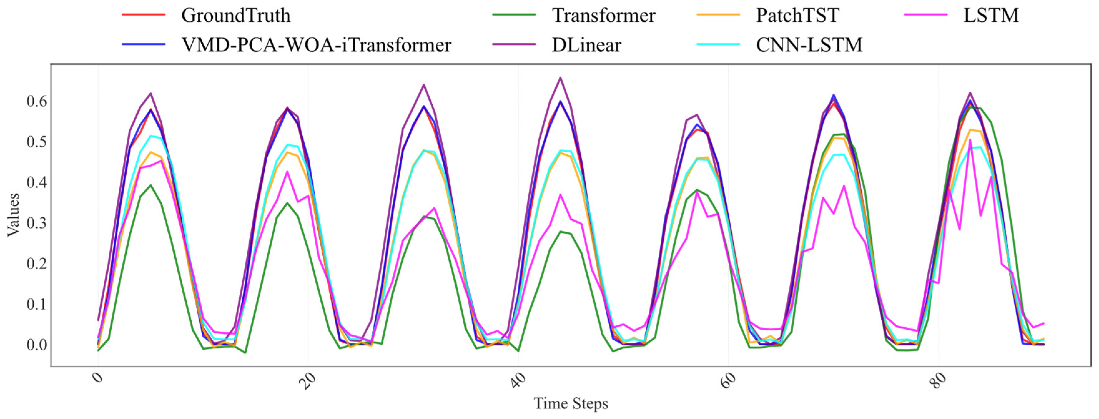
5.1. Multi-Model Comparison

Figure 6 presents a comprehensive boxplot comparison across five key evaluation metrics—R²; MSE; MAE; RMSE; and prediction delay—for the proposed VMD-PCA-WOA-iTransformer model and five state-of-the-art PV forecasting models: Transformer, DLinear, PatchTST, CNN-LSTM, and LSTM. Meanwhile, Figure 7 illustrates the temporal alignment and accuracy of predicted power outputs among these models, offering visual insight into prediction fidelity across the time series.

According to the quantitative results in

Table 5. Comparisons of evaluation metric values for different models.

Model	${\mathit{R}}^2$	MSE	MAE	RMSE	Prediction Delay (ms)
VMD-PCA-WOA-iTransformer	0.8986	0.0088	0.0668	0.0940	0.8160
Transformer	0.8090	0.0211	0.0905	0.1452	143.3779
DLinear	0.8704	0.0143	0.0707	0.1196	0.4475
PatchTST	0.8453	0.0171	0.0963	0.1307	74.4021
CNN-LSTM	0.8444	0.0172	0.0833	0.1310	1.9763
LSTM	0.8165	0.0202	0.0889	0.1423	1.7143

, the proposed VMD-PCA-WOA-iTransformer consistently outperforms all baseline models across every evaluation metric. It achieves the highest R² value of 0.8986, indicating a superior ability to capture the nonlinear dynamics of PV output. In contrast, Transformer and LSTM yield lower R² values of 0.8090 and 0.8165, respectively, highlighting the enhanced fitting capability introduced by the VMD-based decomposition and WOA-optimized parameter tuning. In terms of error control, the proposed model records the lowest MSE (0.0088), MAE (0.0668), and RMSE (0.0940), substantially improving upon the Transformer model (MSE = 0.0211, MAE = 0.0905, RMSE = 0.1452) and PatchTST (MSE = 0.0171, MAE = 0.0963, RMSE = 0.1307). Notably, the MAE of the proposed model is reduced by 26.2% compared to DLinear and by 35.7% compared to PatchTST, which confirms its robustness against local fluctuations and outliers in the time series. Furthermore, while deep learning models such as Transformer and PatchTST suffer from substantial computational latency (e.g., 143.38 ms and 74.40 ms, respectively), the proposed model achieves a remarkably low prediction delay of 0.8160 ms, significantly outperforming all neural network-based counterparts. This confirms its suitability for real-time or embedded PV forecasting scenarios where both accuracy and efficiency are critical.

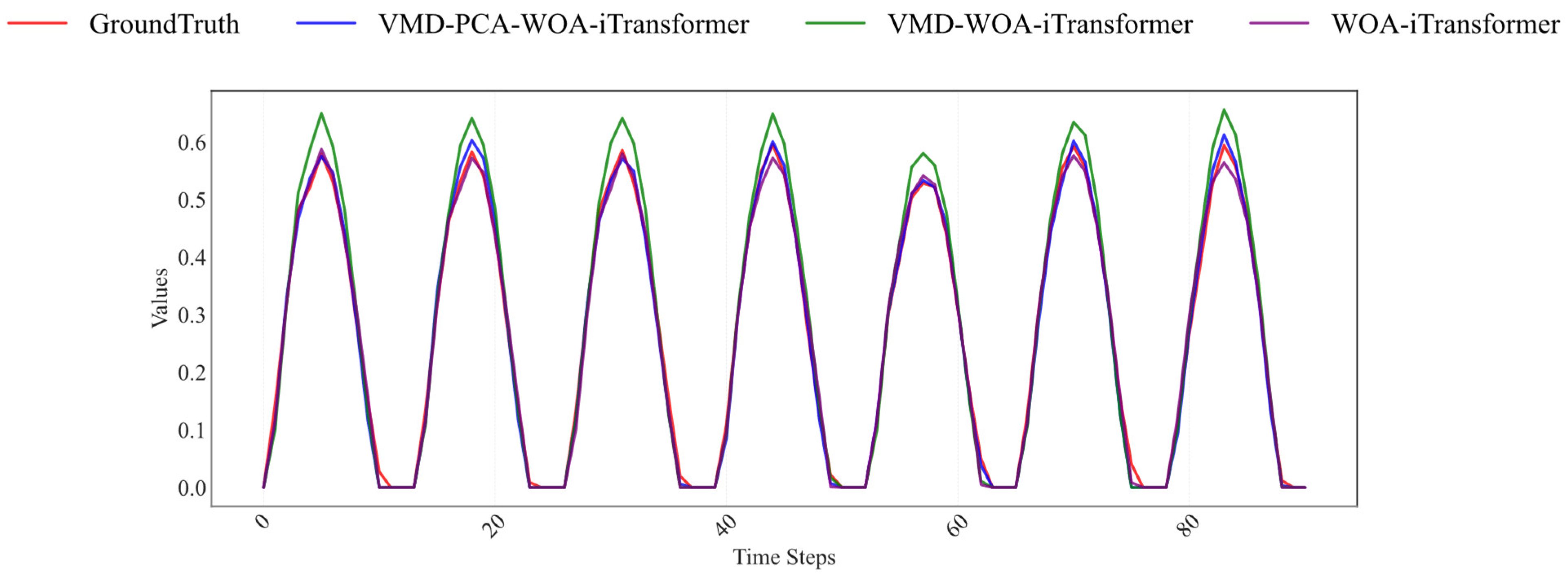
The ablation study results presented in

Table 6. Ablation study results for the VMD-PCA-WOA-iTransformer model.

Model	${\mathit{R}}^2$	MSE	MAE	RMSE
VMD-PCA-WOA-iTransformer	0.8986	0.0088	0.0668	0.0940
VMD-WOA-iTransformer	0.765	0.0275	0.1146	0.1681
WOA-iTransformer	0.8754	0.0091	0.0691	0.0953
iTransformer	0.8476	0.0137	0.0686	0.1169

and illustrated in Figure 8 comprehensively demonstrate the incremental contributions of each component—VMD; PCA; and WOA—to the overall performance of the VMD-PCA-WOA-iTransformer model. The full model exhibits the best predictive performance across all five evaluation metrics, achieving an R² of 0.8986, MSE of 0.0088, MAE of 0.0668, RMSE of 0.0940, and a notably low prediction delay. This underscores the synergistic benefit of combining VMD-based signal decomposition, PCA-based dimensionality reduction, and WOA-driven hyperparameter optimization. Figure 8 further validates these findings by presenting the predicted active power curves for each model variant alongside the actual output, clearly visualizing the extent to which each configuration captures temporal trends and mitigates forecast errors. The full model achieves the closest alignment with ground truth, demonstrating minimal deviation throughout the time series, particularly during peak and transitional periods.

When the VMD component is excluded (as in the PCA-WOA-iTransformer variant), the performance notably deteriorates, with R² dropping to 0.765, MSE increasing to 0.0275, MAE to 0.1146, and RMSE to 0.1681. This highlights the critical role of VMD in enhancing multi-scale feature representation and suppressing noise-induced error propagation. Similarly, removing PCA (in the VMD-WOA-iTransformer variant) results in a modest degradation of performance (R² = 0.8754, MSE = 0.0091, MAE = 0.0691, RMSE = 0.0953), suggesting PCAs importance in eliminating redundant or irrelevant components prior to Transformer-based sequence modeling. The baseline iTransformer model, while competitive (R² = 0.8476, MSE = 0.0137, MAE = 0.0686, RMSE = 0.1169), is consistently outperformed by all integrated variants. These results substantiate the hypothesis that incorporating VMD and PCA enables the model to learn more structured and interpretable temporal features, while WOA optimization fine-tunes the model parameters to achieve superior generalization. In conclusion, both the quantitative data in Table 6 and the predictive fidelity shown in Figure 8 affirm that each module—VMD; PCA; and WOA—plays a non-trivial role in performance enhancement. The VMD-PCA-WOA-iTransformer architecture emerges as the most robust and accurate configuration, capable of delivering precise PV power forecasts under complex temporal dynamics.

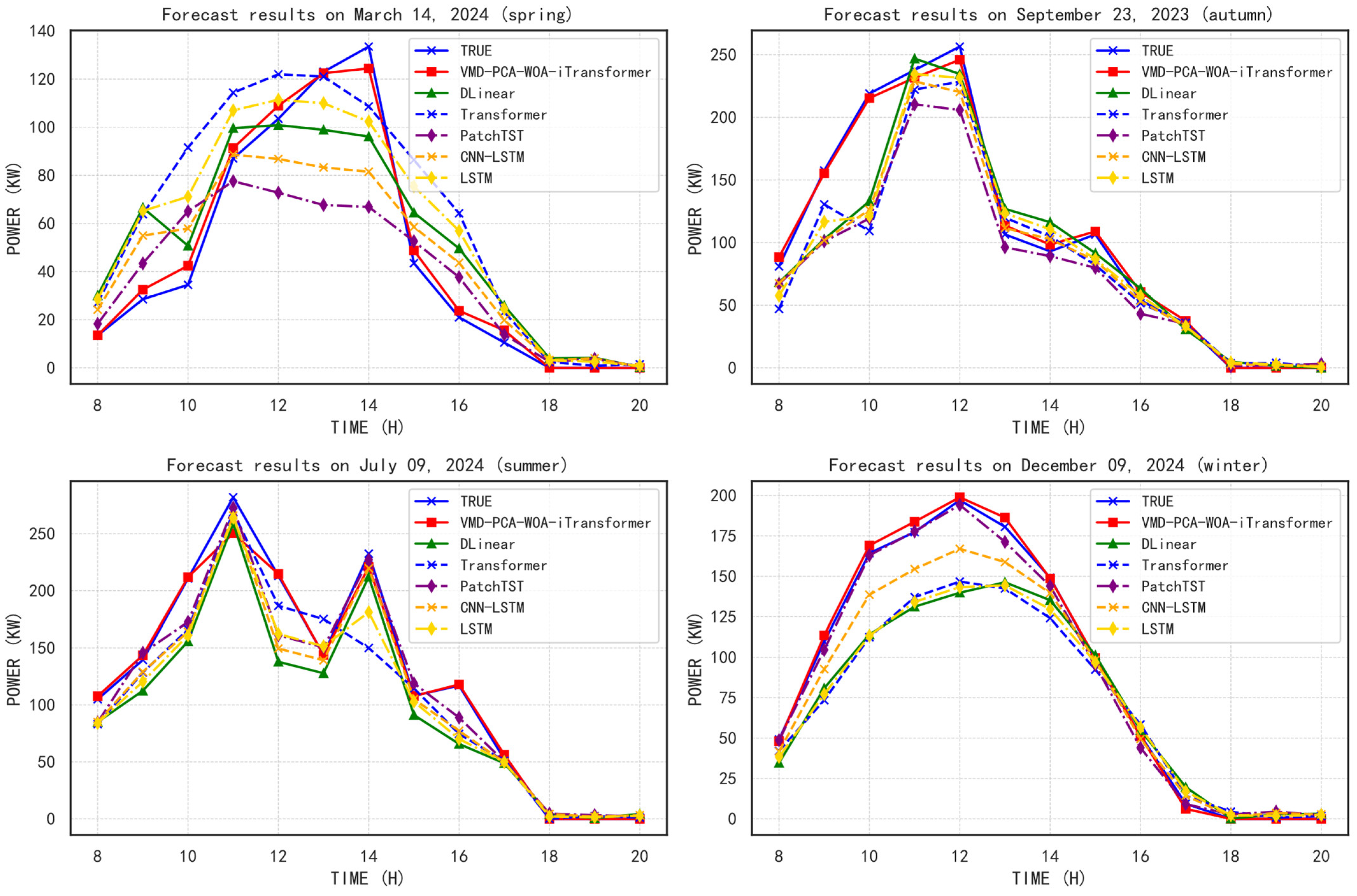
5.2. Performance Under Seasonal Influence

Figure 9 below shows the prediction performance analysis for the four seasons, with the following dates selected as representatives: 14 March 2024 (Spring), 9 July 2024 (Summer), 23 September 2023 (Autumn), and 9 December 2024 (Winter). Corresponding quantitative comparisons are presented in

Table 7. Comparisons of $R^2$ values for different seasons.

$\mathbf{Model}\mathbf{\left(}{\mathit{R}}^2\mathbf{\right)}$	Spring	Summer	Autumn	Winter	Average
VMD-PCA-WOA-iTransformer	0.9304	0.9263	0.9181	0.8983	0.9182
DLinear	0.8000	0.8668	0.8726	0.8517	0.847775
Transformer	0.6369	0.8752	0.8372	0.8526	0.797975
PatchTST	0.6429	0.8455	0.8196	0.8946	0.80065
CNN-LSTM	0.7605	0.8761	0.8580	0.8567	0.837825
LSTM	0.7512	0.8940	0.8623	0.8538	0.8403

,

Table 8. Comparisons of MSE values for different seasons.

Model (MSE)	Spring	Summer	Autumn	Winter	Average
VMD-PCA-WOA-iTransformer	20.8356	90.5199	27.6432	9.8522	37.1127
DLinear	435.3224	1072.7980	956.6163	806.6570	817.8484
Transformer	790.5452	1004.9139	1222.8896	801.4800	954.9572
PatchTST	777.3776	438.7965	1354.6918	19.2834	647.5373
CNN-LSTM	521.3898	675.4770	1066.8322	235.1759	624.6687
LSTM	541.6061	853.8352	1034.4423	794.8751	806.1897

,

Table 9. Comparisons of MAE values for different seasons.

Model (MAE)	Spring	Summer	Autumn	Winter	Average
VMD-PCA-WOA-iTransformer	3.4176	4.4608	4.1872	2.2337	3.5748
DLinear	17.0033	24.3839	20.2324	20.6045	20.5560
Transformer	21.7077	21.8820	21.2343	21.0558	21.4699
PatchTST	19.0904	14.5249	23.6267	3.4605	15.1756
CNN-LSTM	17.3199	17.6317	19.3652	11.5090	16.4564
LSTM	19.1511	21.3828	19.7416	20.6006	20.2190

and

Table 10. Comparisons of RMSE values for different seasons.

Model (RMSE)	Spring	Summer	Autumn	Winter	Average
VMD-PCA-WOA-iTransformer	4.5646	9.5142	5.2577	3.1388	5.6188
DLinear	20.8644	32.7536	30.9292	28.4017	28.2372
Transformer	28.1166	31.7004	34.9698	28.3104	30.7743
PatchTST	27.8815	20.9475	36.8061	4.3913	22.5066
CNN-LSTM	22.8340	25.9899	32.6624	15.3354	24.2054
LSTM	23.2724	29.2205	32.1627	28.1935	28.2123

, covering four performance metrics (R², MSE, MAE, RMSE). A comprehensive analysis of these results reveals the seasonal adaptability and robustness of the proposed VMD-PCA-WOA-iTransformer model relative to five state-of-the-art benchmark models.

In spring, the VMD-PCA-WOA-iTransformer model achieves the highest R² value of 0.9304, significantly outperforming all benchmark models. Notably, the next best model, CNN-LSTM, reaches only 0.7605, indicating the hybrid model’s superior ability to capture the complex variability of spring solar irradiance. The model also records the lowest MSE (20.84), MAE (3.42), and RMSE (4.56), underscoring its high precision and stability under moderately fluctuating seasonal conditions.

During summer, characterized by intense solar radiation and potential intermittency from cloud cover, the hybrid model maintains its top performance with an R² of 0.9263, followed by LSTM (0.8940) and CNN-LSTM (0.8761). Its MSE of 90.52 remains substantially lower than the benchmarks (e.g., DLinear: 1072.80), demonstrating its resilience to high-magnitude data fluctuations. The low MAE (4.46) and RMSE (9.51) further confirm the model’s robustness.

In autumn, which typically presents reduced irradiance and gradual seasonal transitions, the proposed model sustains a leading R² of 0.9181, while other models, such as LSTM (0.8623) and CNN-LSTM (0.8580), exhibit noticeable performance degradation. The VMD-PCA-WOA-iTransformer also achieves the lowest MSE (27.64) and RMSE (5.26), confirming its superior accuracy in handling transitional seasonal patterns.

In winter, where solar radiation is weakest and more erratic due to low sun angles and frequent occlusion, the VMD-PCA-WOA-iTransformer model still ranks first with an R² of 0.8983, outperforming the closest competitors, PatchTST (0.8946) and Transformer (0.8526). Its exceptionally low MSE (9.85), MAE (2.23), and RMSE (3.14) reveal the model’s resilience under challenging low-irradiance conditions.

Overall, across all four seasons, the proposed VMD-PCA-WOA-iTransformer model demonstrates consistent superiority, with the highest average R² (0.9182) and lowest average errors across all metrics (MSE: 37.11, MAE: 3.57, RMSE: 5.62). These results confirm the model’s strong generalization capability, seasonal adaptability, and predictive reliability in diverse environmental scenarios, making it a robust solution for PV power forecasting throughout the year.

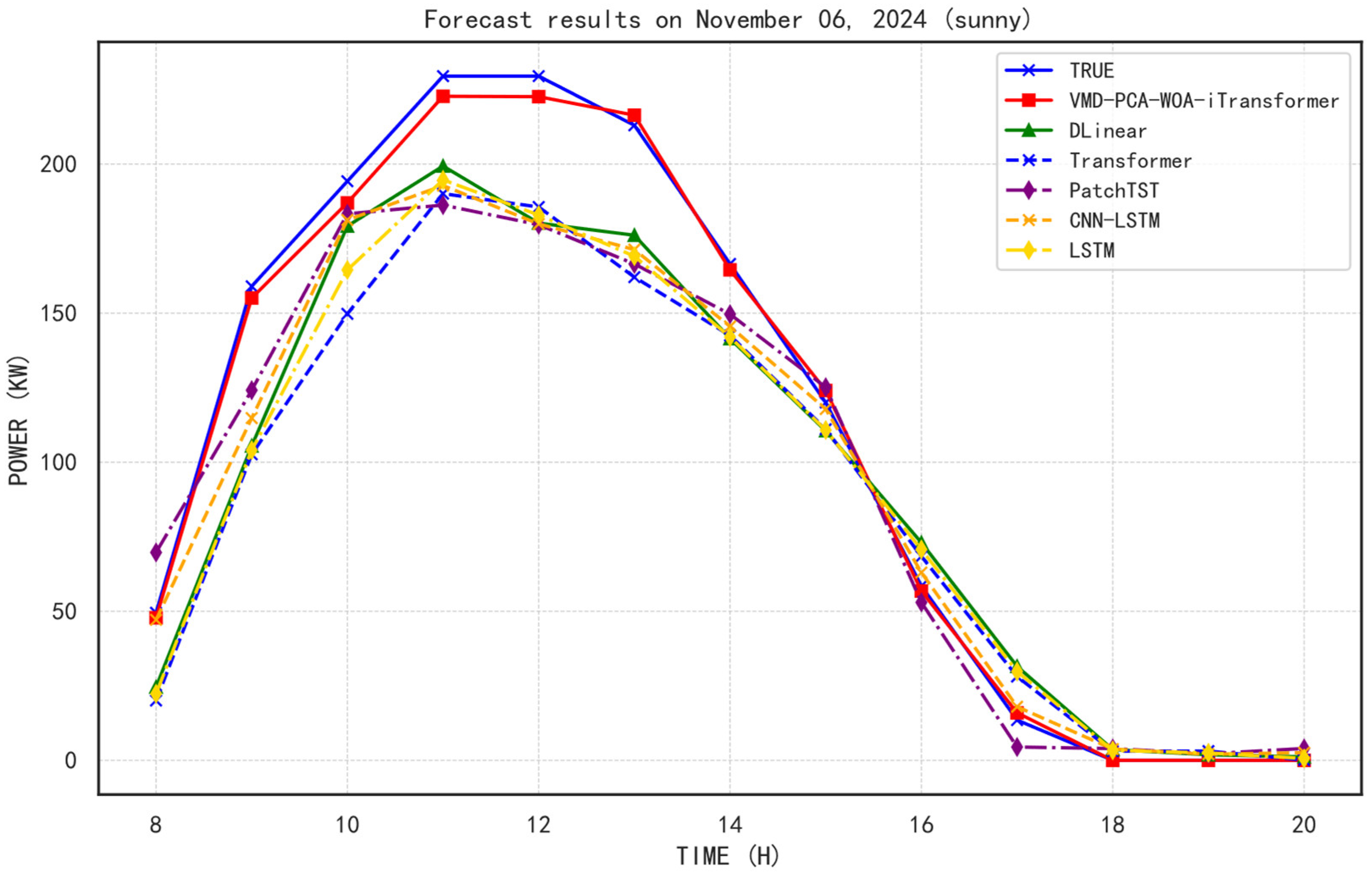
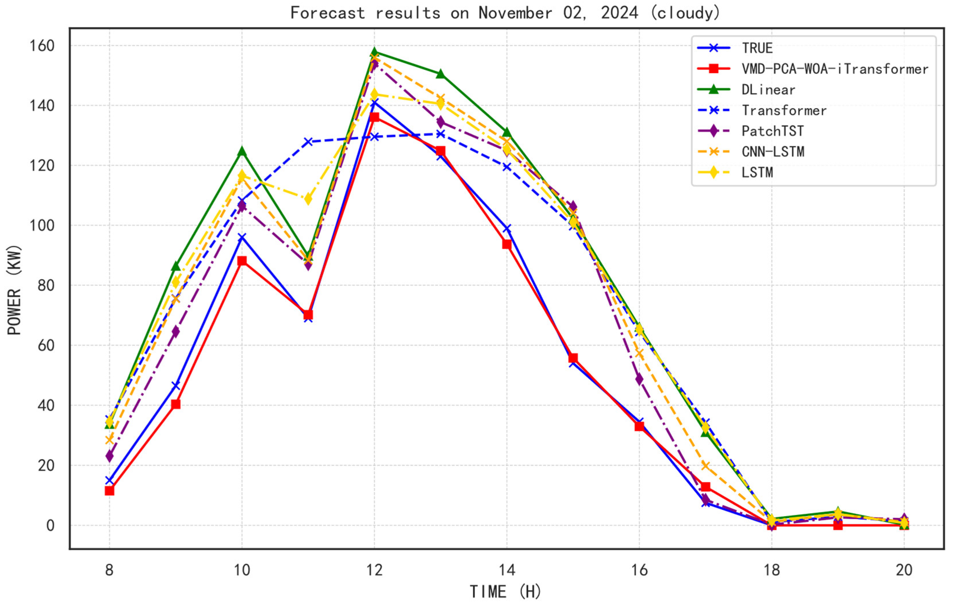
5.3. Performance Under Weather Influence

Figure 10, Figure 11 and Figure 12 illustrate the prediction performance of various models under three weather conditions: sunny, cloudy, and rainy days. Additionally,

Table 11. Comparisons of $R^2$ values for different weather conditions.

$\mathbf{Model}\mathbf{\left(}{\mathit{R}}^2\mathbf{\right)}$	Sunny	Cloudy	Rain	Average
VMD-PCA-WOA-iTransformer	0.9380	0.9231	0.9429	0.9347
DLinear	0.9068	0.6858	0.8955	0.8294
Transformer	0.8741	0.6853	0.8909	0.8168
PatchTST	0.9161	0.8380	0.8648	0.8729
CNN-LSTM	0.9213	0.7797	0.8858	0.8623
LSTM	0.8934	0.7130	0.8937	0.8337

,

Table 12. Comparisons of MSE values for different weather conditions.

Model (MSE)	Sunny	Cloudy	Rain	Average
VMD-PCA-WOA-iTransformer	15.7603	15.6040	81.1722	37.5122
DLinear	745.0240	705.5440	497.4776	649.3485
Transformer	1006.4240	706.6847	519.1332	744.0806
PatchTST	670.8334	363.7092	643.4921	559.3449
CNN-LSTM	629.2323	494.6869	543.5283	555.8158
LSTM	851.8047	644.4078	506.1874	667.4666

,

Table 13. Comparisons of MAE values for different weather conditions.

Model (MAE)	Sunny	Cloudy	Rain	Average
VMD-PCA-WOA-iTransformer	3.0834	3.0300	6.3063	4.1398
DLinear	21.8133	22.6866	17.7171	20.7390
Transformer	25.2516	20.5839	18.1238	21.3198
PatchTST	19.4100	13.6342	19.6176	17.5540
CNN-LSTM	17.5397	18.1604	18.0712	17.9238
LSTM	23.5325	20.7537	17.9204	20.7355

and

Table 14. Comparisons of RMSE values for different weather conditions.

Model (RMSE)	Sunny	Cloudy	Rain	Average
VMD-PCA-WOA-iTransformer	3.9699	3.9502	9.0096	5.6432
DLinear	27.2951	26.5621	22.3042	25.3871
Transformer	31.7242	26.5835	22.7845	27.0307
PatchTST	25.9005	19.0712	25.3671	23.4463
CNN-LSTM	25.0845	22.2416	23.3137	23.5466
LSTM	29.1857	25.3852	22.4986	25.6899

present comprehensive comparisons of R², MSE, MAE, and RMSE values across these weather conditions. The selected representative dates are 6 November 2024 (sunny), 2 November 2024 (cloudy), and 24 November 2024 (rainy), respectively.

Under sunny weather, the VMD-PCA-WOA-iTransformer model exhibits outstanding predictive capability with an R² of 0.9380, the highest among all models, accompanied by the lowest MAE (3.0834) and RMSE (3.9699). This indicates that the model captures the PV generation pattern with high fidelity and low error under optimal illumination. In comparison, the DLinear and Transformer models, although achieving decent R² values (0.9068 and 0.8741, respectively), yield significantly larger MSE and MAE values, demonstrating poorer fit to actual outputs. Other deep learning models such as CNN-LSTM and PatchTST also fall short in terms of accuracy and error control under sunny conditions.

In cloudy weather, where irradiance becomes more variable and less predictable, the superiority of the VMD-PCA-WOA-iTransformer model becomes even more evident. It achieves an R² of 0.9231, maintaining high consistency in prediction. Notably, other models such as DLinear (R² = 0.6858) and Transformer (R² = 0.6853) exhibit severe performance degradation, reflecting their limited adaptability under reduced and unstable solar input. The proposed model also records the lowest MSE (15.6040) and MAE (3.0300), indicating remarkable robustness in uncertain atmospheric scenarios.

Under rainy conditions, typically characterized by extreme fluctuations and lower irradiance, the VMD-PCA-WOA-iTransformer again secures the best performance, with the highest R² of 0.9429 and a remarkably low MAE of 6.3063, compared to substantially higher error metrics in other models (e.g., DLinear MAE = 17.7171, Transformer MAE = 18.1238). Although the RMSE (9.0096) is relatively higher than in other weather conditions due to more pronounced data noise, it remains significantly better than those of competing models, confirming the model’s resilience.

On average across all weather scenarios, the VMD-PCA-WOA-iTransformer achieves the highest R² (0.9347) and the lowest average RMSE (5.6432), substantiating its overall superiority in both accuracy and stability. In contrast, baseline models such as DLinear and Transformer show marked performance drops under non-sunny conditions, indicating their limited generalizability. In summary, the experimental results confirm that the VMD-PCA-WOA-iTransformer model delivers consistently superior performance across all weather conditions, achieving both high prediction accuracy and strong robustness, thus demonstrating considerable potential for real-world deployment in diverse environmental settings.

5.4. Prediction Delay

As shown in Table 5, the proposed VMD-PCA-WOA-iTransformer model achieves a prediction delay of 0.8160 ms, which, although not the shortest among the compared models, remains within a highly acceptable range for practical engineering applications. This delay reflects the intrinsic computational complexity of Transformer-based architectures, which, despite their superior feature extraction and sequence modeling capabilities, typically incur greater inference latency due to multi-head attention mechanisms and deep model depth.

In contrast, the DLinear model exhibits the shortest prediction delay of 0.4475 ms, benefiting from its linear structure that eliminates attention-based computation, resulting in significantly reduced inference time. However, this speed advantage comes at the cost of slightly lower prediction accuracy (R² = 0.8704), indicating a trade-off between computational efficiency and predictive performance. Notably, while the baseline Transformer model achieves a reasonable R² of 0.8090, its prediction delay soars to 143.38 ms, highlighting the inefficiencies introduced by unoptimized self-attention modules when operating without dedicated acceleration or architectural enhancement. Similarly, PatchTST also demonstrates high latency (74.40 ms), despite maintaining competitive accuracy (R² = 0.8453), further reinforcing that transformer variants tend to demand substantial inference time. The CNN-LSTM and LSTM models, with delays of 1.9763 ms and 1.7143 ms, respectively, represent a middle ground between speed and accuracy but fail to match the robustness and predictive precision of the proposed hybrid approach. Overall, the VMD-PCA-WOA-iTransformer offers an optimal balance across accuracy, stability, and delay control, outperforming most models in predictive performance while maintaining manageable inference costs—thereby demonstrating strong applicability for real-time PV forecasting systems.

6. Conclusions

This study presents an integrated PV power forecasting framework (VMD-PCA-WOA-iTransformer) designed for distributed PV power stations under complex meteorological conditions. Through the joint application of signal decomposition, feature reduction, parameter optimization, and time-series modeling, the framework achieves a balanced performance in terms of accuracy, robustness, and computational efficiency.

Extensive experiments conducted under different seasons and weather conditions show that the proposed model outperforms four cutting-edge models and one traditional forecasting model, including DLinear, Transformer, PatchTST, CNN-LSTM, and LSTM. It achieves the highest coefficient of determination (R² = 0.8986) and the lowest prediction delay (0.8160 ms). The model maintains high accuracy across different irradiance levels throughout the year and demonstrates strong generalization ability in sunny, cloudy, and rainy weather. Ablation experiments further confirm the effectiveness of each component: VMD improves feature extraction and denoising, PCA enhances feature correlation and representation, and WOA accelerates convergence and improves training stability.

Although the proposed VMD-PCA-WOA-iTransformer model demonstrates strong performance under diverse meteorological conditions, one notable limitation of this study is that it relies solely on data from a single 372 kWp distributed PV power station located in Guangzhou, China. This may restrict the geographic generalizability of the findings. However, this data selection is driven by the inherent privacy constraints and practical difficulties in obtaining long-term, structured operational datasets from multiple distributed PV systems. Despite this regional data limitation, the proposed framework is intentionally designed with high adaptability and modularity. It demonstrates robust performance in addressing several common challenges encountered in distributed PV systems, including missing or anomalous electrical data and spatial mismatches between meteorological and electrical data sources. These characteristics endow the model with strong theoretical potential for transferability to other geographic regions and various distributed PV scenarios—particularly those in urban or heterogeneous environments with complex spatial distributions and inconsistent data quality.

Furthermore, the current framework employs a static offline training strategy based on historical data, which may limit its adaptability to “Concept Drift” phenomena resulting from seasonal variations, weather fluctuations, and equipment degradation. This limitation may also increase the risk of overfitting in contexts characterized by sparse or noisy input data. Although the VMD component can partially mitigate the problems caused by low-resolution sensors commonly found in real-world PV deployments, the model’s predictive accuracy is still highly dependent on the quality of input data.

Future research will focus on incorporating online learning mechanisms, adaptive temporal attention modules, and ensemble methods with embedded drift detection to improve the model’s robustness and adaptability in non-stationary environments. Additionally, the integration of uncertainty quantification, anomaly detection, and lightweight deployment strategies will further facilitate the practical application of the proposed model on edge devices and within real-time monitoring systems. To improve generalization performance, future work will also aim to include data from multiple distributed PV stations located in different climate zones, with a strong emphasis on data compliance and privacy protection to support broader applicability in real-world scenarios.