Projected Gradient Descent Method for Tropical Principal Component Analysis over Tree Space

Abstract

Tropical Principal Component Analysis (PCA) is an analogue of the classical PCA in the setting of tropical geometry, and applied it to visualize a set of gene trees over a space of phylogenetic trees, which is a union of lower-dimensional polyhedral cones in an Euclidean space with dimension $m(m-1)/2$, where m is the number of leaves. In this paper, we introduce a projected gradient descent method to estimate the tropical principal polytope over the space of phylogenetic trees, and we apply it to an Apicomplexa dataset. With computational experiments against Markov Chain Monte Carlo (MCMC) samplers, we show that our projected gradient descent method yields a lower sum of tropical distances between observations and their projections onto the estimated best-fit tropical polytope, compared with the MCMC-based approach.

1. Introduction

Phylogenomics is a relatively new field that applies tools from phylogenetics to genome data. One of the key tasks in phylogenomics is to analyze gene trees, which are phylogenetic trees representing the evolutionary histories of genes in the genome. In this work, we use an unsupervised learning method to visualize how gene trees are distributed over the space of phylogenetic trees, that is, the set of all possible phylogenetic trees with a fixed set of labels for all leaves.

A phylogenetic tree T on a given set of leaves $\left[m\right]:=\{1,\dots ,m\}$ is a weighted tree in which the internal nodes in T are unlabeled, their leaves X are labeled, and their branch lengths represent evolutionary time and mutation rates. In phylogenetics, a phylogenetic tree on the set of species $\left[m\right]$ represents their evolutionary history. In phylogenomics, we construct a phylogenetic tree from an alignment or sequence data for each gene in a given genome. A phylogenetic tree reconstruced from a gene alignment is called a gene tree. Since different genes may have distinct evolutionary histories, gene trees can vary in topology and branch lengths. Thus, it is a statistical challenge to analyze a set of phylogenetic trees.

When conducting statistical analysis on a set of phylogenetic trees, we represent each tree as a vector in a high-dimensional vector space. One common method is to compute all pairwise distances between two distinct leaves in $\left[m\right]$, resulting in ${\mathbb{R}}^{\left({\displaystyle \genfrac{}{}{0pt}{}{m}{2}}\right)}$. However, not every vector in ${\mathbb{R}}^{\left({\displaystyle \genfrac{}{}{0pt}{}{m}{2}}\right)}$ corresponds to a valid phylogenetic tree on $\left[m\right]$. In 1974, Buneman showed [1] that a vector derived from all possible pairwise distances between leaves in $\left[m\right]$ must satisfy the four-point conditions to represent a phylogenetic tree. For an equidistant tree—namely, a rooted phylogenetic tree in which the total edge weight from the root to each leaf in $\left[m\right]$ is equal (see Definition 9)—the vector must satisfy the three-point condition to correspond to the phylogenetic tree (Theorem 1).

In 2006, Ardila and Klivans showed that the space of all phylogenetic trees on $\left[m\right]$ is a union of $m-2$ dimensional cones in ${\mathbb{R}}^{\left({\displaystyle \genfrac{}{}{0pt}{}{m}{2}}\right)}$, and that this space is not classically convex [2]. Therefore, classical statistical methods cannot be directly applied to a set of phylogenetic trees, as these methods assume a Euclidean sample space.

However, Ardila and Klivans also showed that the space of equidistant trees—rooted phylogenetic trees on $\left[m\right]$ as defined in Definition 9—is a tropical Grasmaniann. So, the space of equidistant trees on $\left[m\right]$ is tropically convex and forms a tropical linear space with the max-plus algebra over the tropical projective space. Therefore, we can apply tropical linear algebra to perform statistical analysis on the space of equidistant trees on $\left[m\right]$.

In 2019, Yoshida et al. introduced tropical principal component analysis (PCA), an analogue of a classical PCA from the perspective of tropical geometry, to visualize how gene trees are distributed over the space of equidistant trees on $\left[m\right]$ using max-plus algebra [3]. For $s\le \left({\displaystyle \genfrac{}{}{0pt}{}{m}{2}}\right)$, they defined the $(s-1)$-th order tropcial principal polytope, or the best-fit tropical polytope with s vertices, whose vertices serve as analogues of the classical first s principal components.They showed that computing these vertices can be formulated as a mixed integer linear programming problem, as shown in Problem 1 [3]. Later, Page et al.  developed a Markov Chain Monte Carlo (MCMC) method to estimate the vertices of the tropical principal polytope from a set of gene trees.

In this work, inspired by the recent work of tropical gradient descent defined in [4], we introduce a projected gradient descent method to compute the set of vertices of the tropical principal polytope from a set of gene trees. We compute subgradients in order to find the optimal solution for the mixed integer programming problem in order to compute the tropical principal polytope shown in Theorem 3. Then, we apply our novel method to Apicomplexa data from [5], and our experiments using the R package TML version 2.3.0 [6] show that our method outperforms existing approaches in terms of computational time and cost function.

This paper is organized as follows. In Section 2, we introduce the basics of tropical geometry. In Section 3, we review the notions of metrics and ultrametrics, and discuss the isometry between the space of equidistant trees on $\left[m\right]$ and the space of ultrametrics on the finite set $\left[m\right]$, based on results by Buneman [1]. In Section 4, we present tropical PCA and the s-th order tropical principal polytope for $s\le e$, where $e:=\left({\displaystyle \genfrac{}{}{0pt}{}{m}{2}}\right)$. Section 5 provides experimental results on the Apicomplexa dataset from [5].

2. Tropical Basics

In this section, we introduce the basics of tropical geometry to be used for our main results. Let $\mathbf{1}$$=(1,\dots ,1)\in {\mathbb{R}}^e$. Then, through this paper, we consider the tropical projective torus, ${\mathbb{R}}^e/\mathbb{R}\mathbf{1}$ which is isomorphic to ${\mathbb{R}}^{e-1}$. This means that ${\mathbb{R}}^e/\mathbb{R}\mathbf{1}$ is equivalent to a hyperplane in ${\mathbb{R}}^e$. This implies that for a point $x:=(x_1,\dots ,x_e)\in {\mathbb{R}}^e/\mathbb{R}\mathbf{1}$,

$$(x_1,\dots ,x_e)=(x_1+c,\dots ,x_e+c)$$

where $c\in \mathbb{R}$. See [7] for more details.

Throughout this paper, we consider tropically convex sets defined by the max-plus algebra provided in Definition 1.

Definition 1 (Tropical Arithmetic Operations). 

The tropical semiring $(\mathbb{R}\cup \{-\infty \},\oplus ,\odot )$ is defined using the following tropical addition ⊕ and multiplication ⊙:

$$a\oplus b:=max\{a,b\},a\odot b:=a+b$$

for any $a,b\in \mathbb{R}\cup \{-\infty \}$.

Remark 1. 

$-\infty$ is the identity element under addition ⊕ and 0 is the identity element under multiplication ⊙ over $(\mathbb{R}\cup \{-\infty \},\oplus ,\odot )$.

Definition 2 (Tropical Scalar Multiplication and Vector Addition). 

For any $a,b\in \mathbb{R}\cup \{-\infty \}$ and for any $v=(v_1,\dots ,v_e),w=(w_1,\dots ,w_e)\in {(\mathbb{R}\cup \{-\infty \})}^e$, the tropical scalar multiplication and tropical vector addition are defined as:

$$a\odot v\oplus b\odot w:=(max\{a+v_1,b+w_1\},\dots ,max\{a+v_e,b+w_e\}).$$

Definition 3 (Generalized Hilbert Projective Metric). 

For any points $v:=(v_1,\dots ,v_d),w:=(w_1,\dots ,w_e)\in {\mathbb{R}}^e/\mathbb{R}\mathbf{1}$, the tropical metric, $d_{\mathrm{tr}}$, between v and w, is defined as:

$$d_{\mathrm{tr}}(v,w):=\underset{i\in \{1,\dots ,e\}}{max}\left\{v_i-w_i\right\}-\underset{i\in \{1,\dots ,e\}}{min}\left\{v_i-w_i\right\}.$$

(1)

Remark 2. 

The tropical metric $d_{\mathrm{tr}}$ is the metric over ${\mathbb{R}}^e/\mathbb{R}\mathbf{1}$.

Definition 4. 

A subset $S\subset {\mathbb{R}}^e$ is called tropically convex if it contains the point $a\odot x\oplus b\odot y$ for all $x,y\in S$ and all $a,b\in \mathbb{R}$. The tropical convex hull or tropical polytope, $\mathrm{tconv}\left(V\right)$, of a given finite subset $V\subset {\mathbb{R}}^e$ is the smallest tropically convex set containing $V\subset {\mathbb{R}}^e$. In addition, $\mathrm{tconv}\left(V\right)$ can be written as the set of all tropical linear combinations

$$\mathrm{tconv}\left(V\right)=\{a_1\odot v_1\oplus a_2\odot v_2\oplus \cdots \oplus a_r\odot v_r:v_1,\dots ,v_r\in Vand{a}_1,\dots ,a_r\in \mathbb{R}\}.$$

Any tropically convex subset S of ${\mathbb{R}}^e$ is closed under tropical scalar multiplication, $\mathbb{R}\odot S\subseteq S$, i.e., if $x\in S$, then $x+c·\mathbf{1}\in S\mathit{for}\mathit{all}c\in \mathbb{R}$. Thus, the tropically convex set S is identified as its quotient in the tropical projective torus ${\mathbb{R}}^e/\mathbb{R}\mathbf{1}$.

Definition 5 

(Max-tropical Hyperplane [8]). A max-tropical hyperplane $H_{\omega }^{max}$ is the set of points $x\in {\mathbb{R}}^e/\mathbb{R}\mathbf{1}$, such that

$$\underset{i\in \{1,\dots ,e\}}{max}\{x_i+{\omega }_i\}$$

(2)

is attained at least twice, where $\omega :=({\omega }_1,\dots ,{\omega }_e)\in {\mathbb{R}}^e/\mathbb{R}\mathbf{1}$.

Definition 6 

(Min-tropical Hyperplane [8]). A min-tropical hyperplane $H_{\omega }^{min}$ is the set of points $x\in {\mathbb{R}}^d/\mathbb{R}\mathbf{1}$, such that

$$\underset{i\in \{1,\dots ,e\}}{min}\{x_i+{\omega }_i\}$$

(3)

is attained at least twice, where $\omega :=({\omega }_1,\dots ,{\omega }_e)\in {\mathbb{R}}^e/\mathbb{R}\mathbf{1}$.

Remark 3. 

A min-tropical hyperplane $H_{\omega }^{min}$ and a max-tropical hyperplane $H_{\omega }^{max}$ are tropically convex over ${(R\cup \{-\infty \})}^e/\mathbb{R}\mathbf{1}$.

Definition 7 

(Max-tropical Sectors from Section 5.5 in [8]). For $i\in \left[e\right]$, the i-th open sector of $H_{\omega }^{max}$ is defined as

$$S_{\omega }^{max,i}:=\{\mathbf{x}\in {\mathbb{R}}^e/\mathbb{R}\mathbf{1}|{\omega }_i+x_i>{\omega }_j+x_j,\forall j\ne i\}.$$

(4)

and the i-th closed sector of $H_{\omega }^{max}$ is defined as

$${\overline{S}}_{\omega }^{max,i}:=\{\mathbf{x}\in {\mathbb{R}}^e/\mathbb{R}\mathbf{1}|{\omega }_i+x_i\ge {\omega }_j+x_j,\forall j\ne i\}.$$

(5)

Definition 8 

(Min-tropical Sectors). For $i\in \left[d\right]$, the i-th open sector of $H_{\omega }^{min}$ is defined as

$$S_{\omega }^{min,i}:=\{\mathbf{x}\in {\mathbb{R}}^d/\mathbb{R}\mathbf{1}|{\omega }_i+x_i<{\omega }_j+x_j,\forall j\ne i\},$$

(6)

and the i-th closed sector of $H_{\omega }^{min}$ is defined as

$${\overline{S}}_{\omega }^{min,i}:=\{\mathbf{x}\in {\mathbb{R}}^d/\mathbb{R}\mathbf{1}|{\omega }_i+x_i\le {\omega }_j+x_j,\forall j\ne i\}.$$

(7)

3. Space of Phylogenetic Trees

A phylogenetic tree is a rooted or unrooted tree whose exterior nodes have unique labels, whose interior nodes do not have labels, and whose edges have non-negative weights. In this paper, we focus on an equidistant tree that is a rooted phylogenetic tree, such that a total weight on the path from its root to each leaf on the tree has the same total weight. Let $\left[m\right]:=\{1,\dots ,m\}$ be the set of leaf labels on an equidistant tree T.

Definition 9. 

An equidistant tree T on $\left[m\right]$ is a rooted phylogenetic tree on $\left[m\right]$, such that the total weight from the root to each leaf $i\in \left[m\right]$ is equal to a constant $h>0$ for all $i\in \left[m\right]$. h is the height of T.

Example 1. 

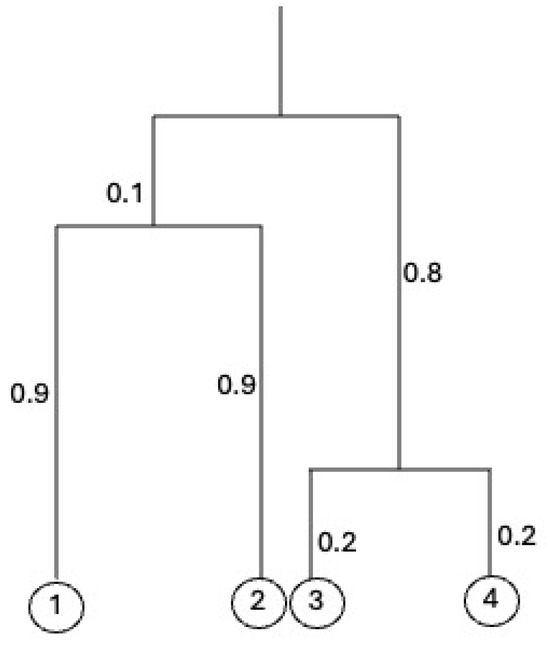
Figure 1 shows an equidistant tree a height 1 on $\left[4\right]:=\{1,2,3,4\}$.

Figure 1. An equidistant tree with $\left[4\right]:=\{1,2,3,4\}$ from Example 1. The height of the tree is 1.

Suppose $D(i,j)$ is the total weight on the unique path from a leaf $i\in \left[m\right]$ and a leaf $j\in \left[m\right]$ on a phylogenetic tree T. Then, $D=(D(1,2),D(1,3),\dots ,D(m-1,m))\in {\mathbb{R}}_{\ge 0}^e$, where $e:=\left({\displaystyle \genfrac{}{}{0pt}{}{m}{2}}\right)$, is a metric, that is, D satisfies

$$\begin{array}{c}\hfill D(i,j)\le D(i,k)+D(k,j)\\ \hfill D(i,j)=D(j,i)\\ \hfill D(i,j)=0\end{array}$$

for all $i,j,k\in \left[m\right]$. The metric D is the tree metric of a phylogenetic tree T.

If metric D satisfies

$$\begin{array}{c}\hfill max\left\{D\right(i,j),D(i,k),D(k,j\left)\right\}\end{array}$$

and this maximum is achieved at least twice for distinct $i,j,k\in \left[m\right]$, then D is called an ultrametric. Suppose $D(i,j)$ is the total weight of the path from $i,i\in \left[m\right]$ from an equidistant tree T, then we have the following theorem.

Theorem 1 

(noted in [1]). Suppose we have an equidistant tree T with a leaf label set $\left[m\right]$ and D as its tree metric. Then, D is an ultrametric if and only if T is an equidistant tree. In addition, we can uniquely reconstruct T from D.

Using Theorem 1, we consider the space of ultrametrics on $\left[m\right]$ as the space of phylogenetic trees, which is the set of all possible equidistant trees with the leaf set $\left[m\right]$. Let ${\mathcal{U}}_m$ be the space of ultrametrics on $\left[m\right]$.

With tropical geometry, it can be shown that ${\mathcal{U}}_m$ is a tropical subspace over the tropical projective space ${(\mathbb{R}\cup \{-\infty \})}^e/\mathbb{R}\mathbf{1}$. Let $L_m$ denote the subspace of ${\mathbb{R}}^e$, defined by the linear equations, such that $x_{ij}-x_{ik}+x_{jk}=0$ for $1\le i<j<k\le m$. The tropicalization $\mathrm{Trop}\left(L_m\right)\subseteq {(\mathbb{R}\cup \{-\infty \})}^e/\mathbb{R}\mathbf{1}$ is the tropical linear space consisting of points $(u_{12},u_{13},\dots ,u_{m-1,m})$, such that, for any $max(u_{ij},u_{ik},u_{jk})$, the maximum of $i,j,k\in \left[m\right]$ is achieved at least twice.

In addition, it is important to note that the tropical linear space $\mathrm{Trop}\left(L_m\right)$ corresponds to the graphic matroid of the complete graph $K_m$.

Theorem 2 

(Theorem 2.18 in [3]). The image of ${\mathcal{U}}_m$ in the tropical projective torus ${\mathbb{R}}^e/\mathbb{R}\mathbf{1}$ coincides with $\mathit{Trop}\left(L_m\right)$.

Projection onto Tree Space

In tropical geometry, it is well-known that ${\mathcal{U}}_m$ is the support of a pointed simplicial fan of dimension $m-2$ and it has $2^m-m-2$ rays, defined as clade metrics [2].

Definition 10. 

Suppose we have an equidistant phylogenetic tree T with leaf set $\left[m\right]$. A clade of T with leaves $\sigma \subset \left[m\right]$ is the equidistant subtree of T formed by including all common ancestral interior nodes of combinations of leaves in σ, while excluding any common ancestors that involve leaves from $X-\sigma$ in T, along with the edges in T that connect these interior nodes to the leaves in σ.

We note that a clade of an equidistant tree T with leaf set $\sigma \subset \left[m\right]$ is a subtree of T with leaves $\sigma$. Feichtner showed that each topology of equidistant trees can be encoded by a nested set, that is, a set of clades $\{{\sigma }_1,\dots ,{\sigma }_C\}$, where $C\in \{1,\dots ,m-2\}$, such that

$${\sigma }_i\subset {\sigma }_j,\mathrm{or} {\sigma }_j\subset {\sigma }_i,\mathrm{or} {\sigma }_i\cap {\sigma }_j=\varnothing$$

for all $1\le i\le j\le C$ and $|{\sigma }_k| \ge 2$ for all $k=1,\dots ,C$ [9].

Definition 11 

(Clade Ultrametrics). We consider an equidistant tree T on the leaf set $\left[m\right]$. Let $\sigma \subset \left[m\right]$ be a proper subset of $\left[m\right]$ with at least two elements. Let $D_{\sigma }:=(D_{\sigma }(1,2),\dots ,D_{\sigma }(m-1,m))\in {\mathcal{U}}_m$, such that

$$D_{\sigma }(i,j)=\left\{\begin{array}{cc}0\hfill & if i,j\in \sigma \hfill \\ 1\hfill & otherwise.\hfill \end{array}\right.$$

Then, $D_{\sigma }$ is called a clade ultrametric.

We note that Ardila and Klivans showed that the set of clade ultrametrics forms a set of generators—i.e., rays—of a pointed simplicial fan of dimension $m-2$, in terms of classical arithmetic in Euclidean geometry. In this paper, we use an extreme clade ultrametric, which is an analogue of a clade ultrametric defined using the max-plus algebra. This is done by replacing the identity element of classical addition with the identity of tropical addition ⊕ (namely, replacing 0 with $-\infty$), and replacing the identity element of classical multiplication with that of tropical multiplication ⊙ (namely, replacing 1 with 0).

Definition 12 

(Extreme Clade Ultrametrics). We consider an equidistant tree T on the leaf set $\left[m\right]$. Let $\sigma \subset \left[m\right]$ be a proper subset with at least two elements. Let $D_{\sigma }:=(D_{\sigma }(1,2),\dots ,D_{\sigma }(m-1,m))\in {\mathcal{U}}_m$, such that

$$D_{\sigma }(i,j)=\left\{\begin{array}{cc}-\infty \hfill & if i,j\in \sigma \hfill \\ 0\hfill & otherwise.\hfill \end{array}\right.$$

Then, $D_{\sigma }$ is called an extreme clade ultrametric.

Remark 4. 

In polyhedral geometry, a polyhedral cone generated by a set of rays $V=\{v^1,\dots ,v^k\}\subset {\mathbb{R}}^{e-1}$ is defined as

$$C\left(V\right)=\left\{x\in {\mathbb{R}}^{e-1}|x=\sum _{i=1}^k{\alpha }_i{v}^i,{\alpha }_i\ge 0 for all i=1,\dots ,k\right\}.$$

We replace classical addition with ⊕ and classical multiplication with ⊙ for $V=\{v^1,\dots ,v^k\}\subset {\mathbb{R}}^e/\mathbb{R}\mathbf{1}\cong {\mathbb{R}}^{e-1}$; thus, we have

$$Trop\left(C\left(V\right)\right)=\left\{x\in {\mathbb{R}}^e/\mathbb{R}\mathbf{1}|x=\underset{i=1}{\overset{k}{⨁}}{\alpha }_i\odot v^i,{\alpha }_i\in \mathbb{R} for all i=1,\dots ,k\right\}$$

which is a tropical polytope defined by V.

Proposition 1 

([10]). The set of all extreme clade ultrametrics, ${\mathcal{U}}_m^{\infty }$, is a generating set of ${\mathcal{U}}_m$ in terms of max-plus algebra.

Proposition 1 is a tropical geometric analogue of the simplicial complex result by Ardila and Klivans in [2], obtained by replacing classical addition with ⊕ and classical multiplication with ⊙.

Definition 13 

(Projection Map [10]). The tropical projection map to ultrametric tree space ${\pi }_{{\mathcal{U}}_m}:{(\mathbb{R}\cup \{-\infty \})}^e/\mathbb{R}\mathbf{1}\to {\mathcal{U}}_m$ is given by

$${\pi }_{{\mathcal{U}}_m}\left(x\right)=\underset{v\in {\mathcal{U}}_m^{\infty }}{⨁}{\lambda }_v\odot v,{\lambda }_v=\underset{j:v_j=0}{min}\left\{x_j\right\}$$

for $x:=(x_1,\dots ,x_e)\in {\mathbb{R}}^e/\mathbb{R}\mathbf{1}$.

Proposition 2 

([10]). For all $x\in {\mathbb{R}}^e/\mathbb{R}\mathbf{1}$, we have

$$d_{\mathrm{tr}}(x,x^{\prime })\le d_{\mathrm{tr}}(x,y)$$

for all $y\in {\mathcal{U}}_m$, and where $x^{\prime }={\pi }_{{\mathcal{U}}_m}\left(x\right)$ is defined by Definition 13.

The following proposition is key to the projected gradient methods we proposed in Section 4.

Proposition 3 

(Lemma 19, [11]). The projection map ${\pi }_{{\mathcal{U}}_m}\left(x\right)$ is non-expansive in terms of $d_{\mathrm{tr}}$, i.e.,

$$d_{\mathrm{tr}}({\pi }_{{\mathcal{U}}_m}\left(u\right),{\pi }_{{\mathcal{U}}_m}\left(v\right))\le d_{\mathrm{tr}}(u,v)$$

for all $u,v\in {\mathbb{R}}^e/\mathbb{R}\mathbf{1}$.

Remark 5. 

The projection map ${\pi }_{{\mathcal{U}}_m}$ is equivalent to the single linkage hierarchical clustering method [12]. Therefore, in the computational experiment described in Section 5, we use a single linkage hierarchical clustering method to projecting a subgradient.

4. Tropical Principal Component Analysis

Yoshida et al. introduced the notion of tropical principal component analysis (PCA), an analysis based on the best-fit tropical hyperplane or tropical polytope [3]. In particular, they applied tropical PCA using tropical polytopes to samples of ultrametrics within the space of ultrametrics. In this section, we consider ${\mathcal{U}}_m\subset {\mathbb{R}}^e/\mathbb{R}\mathbf{1}$, where m is the number of leaves and $e=\left({\displaystyle \genfrac{}{}{0pt}{}{m}{2}}\right)$. Suppose we have a sample $\mathcal{S}:=\{u_1,\dots u_n\}\subset {\mathcal{U}}_m$.

Definition 14 

(Definition 3.1 in [13]). The $(s-1)$-th order tropical principal polytope $\mathcal{P}$ minimizes

$$\sum _{i=1}^n{d}_{\mathrm{tr}}(u_i,w_i)$$

where $w_i$ is the projection onto a tropical polytope $\mathcal{P}$ with s many vertices, that is

$$d_{\mathrm{tr}}(u_i,w_i)\le d_{\mathrm{tr}}(u_i,x)$$

for all $x\in \mathcal{P}$ for $\mathcal{S}:\{u_1,\dots u_n\}$, which is called the $(s-1)$th-order tropical principal component polytope of the sample $\mathcal{S}$. The s vertices of the tropical principal component polytope $\mathcal{P}$ are called the $(s-1)$th order tropical principal components, or equivalently, the best-fit tropical polytope with s vertices.

Remark 6. 

The 0-th tropical principal polytope is a tropical Fermat–Weber point of a sample $\mathcal{S}$ with respect to $d_{\mathrm{tr}}$. A tropical Fermat–Weber point of $\mathcal{S}$ with respect to $d_{\mathrm{tr}}$ is defined as

$$x^{*}:=\underset{x\in {\mathbb{R}}^e/\mathbb{R}\mathbf{1}}{arg\; min}\sum _{i=1}^n{d}_{\mathrm{tr}}(x,u_i).$$

A tropical Fermat–Weber point of $\mathcal{S}$ with respect to $d_{\mathrm{tr}}$ is not necessarily unique, and the set of all tropical Fermat–Weber points forms both a classical polytope and a tropical polytope [14].

In this paper, we focus on the $(s-1)$-th order principal components over ${\mathcal{U}}_m\subset {\mathbb{R}}^e/\mathbb{R}\mathbf{1}$ for $s>1$. Our problem can be written as follows:

Problem 1. 

We seek a solution for the following optimization problem:

$$\underset{D^{\left(1\right)},\dots ,D^{\left(s\right)}\in {\mathcal{U}}_m}{min}\sum _{i=1}^n{d}_{\mathrm{tr}}(u_i,w_i)$$

where

$$w_i={\lambda }_1^i\odot D^{\left(1\right)}\oplus \dots \oplus {\lambda }_s^i\odot D^{\left(s\right)},\mathrm{where}{\lambda }_k^i=\min (u_i-D^{\left(k\right)}),$$

(8)

and

$$d_{\mathrm{tr}}(u_i,w_i)=max\left\{\right|u_i\left(k\right)-w_i\left(k\right)-u_i\left(l\right)+w_i\left(l\right)|:1\le k<l\le e\}$$

(9)

with

$$u_i=(u_i\left(1\right),\dots ,u_i\left(e\right))\mathrm{and}{w}_i=(w_i\left(1\right),\dots ,w_i\left(e\right)).$$

(10)

Remark 7 

(Proposition 4.2 in [3]). Problem 1 can be formulated as a mixed integer programming problem.

In this section, we consider subgradients of Problem 1. Here, we are interested in computing

$${\displaystyle \frac{\partial d_{\mathrm{tr}}(u_i,w_i)}{\partial D^{\left(k\right)}}}.$$

First, we notice that

$$\begin{array}{ccc}\hfill {\displaystyle \frac{\partial d_{\mathrm{tr}}(u_i,w_i)}{\partial D^{\left(k\right)}}}& =& {\displaystyle \frac{\partial d_{\mathrm{tr}}(u_i,w_i)}{\partial w_i}}{\displaystyle \frac{\partial w_i}{\partial D^{\left(k\right)}}}\hfill \end{array}$$

by the product rule.

Let

$${\delta }_{ij}=\left\{\begin{array}{cc}1\hfill & \mathrm{i}\mathrm{f} i=j\hfill \\ 0\hfill & \mathrm{o}\mathrm{t}\mathrm{h}\mathrm{e}\mathrm{r}\mathrm{w}\mathrm{i}\mathrm{s}\mathrm{e}.\hfill \end{array}\right.$$

be Kronecker’s Delta. Then, we have the following lemma:

Lemma 1 

(Lemma 10 in [14]). For any two points $x,p\in {\mathbb{R}}^e/\mathbb{R}\mathbf{1}$, the gradient at x of the tropical distance between x and p is given by

$${\displaystyle \frac{\partial d_{\mathrm{tr}}(p,x)}{\partial x\left(l^{\prime }\right)}}=\left({\delta }_{l^{\prime }t}-{\delta }_{l^{\prime }{t}^{\prime }}\mid x\in S_{-p}^{max,t}\cap S_{-p}^{min,t^{\prime }}\right).$$

(11)

provided there are no ties in $(x-p)$, which ensures that the min- and max-sectors are uniquely identifiable; that is, the point x is inside of open sectors and not on the boundary of $H_{-p}$.

Also, we notice that

$$\begin{array}{ccc}\hfill w_i\left(l\right)& =& max\left[\left(\underset{j}{min}(u_i\left(j\right)-D^{\left(1\right)}\left(j\right))\mathbf{1}+D^{\left(1\right)}\right)\left(l\right),\dots ,\left(\underset{j}{min}(u_i\left(j\right)-D^{\left(s\right)}\left(j\right))\mathbf{1}+D^{\left(s\right)}\right)\left(l\right)\right],\hfill \end{array}$$

for $l=1,\dots ,e$.

Lemma 2. 

$${\displaystyle \frac{\partial w_i\left(l^{\prime }\right)}{\partial D^{\left(k\right)}\left(l\right)}}=\left\{\begin{array}{cc}-1\hfill & if{\mathrm{argmax}}_{k^{\prime }}\left\{\left(D^{\left(k^{\prime }\right)}+\underset{j}{min}(u_i\left(j\right)-D^{\left(k^{\prime }\right)}\left(j\right))\mathbf{1}\right)\left(l^{\prime }\right)\right\}=k,\hfill \\ \hfill & \underset{j}{min}(u_i\left(j\right)-D^{\left(k\right)}\left(j\right))=l, and l^{\prime }\ne l,\hfill \\ 1\hfill & if{\mathrm{argmax}}_{k^{\prime }}\left\{\left(D^{\left(k^{\prime }\right)}+\underset{j}{min}(u_i\left(j\right)-D^{\left(k^{\prime }\right)}\left(j\right))\mathbf{1}\right)\left(l^{\prime }\right)\right\}=k,\hfill \\ \hfill & \underset{j}{min}(u_i\left(j\right)-D^{\left(k\right)}\left(j\right))\ne l, and l^{\prime }=l,\hfill \\ 0\hfill & otherwise,\hfill \end{array}\right.$$

(12)

for $i=1,\dots ,n$, $k=1,\dots ,s$, and for $l=1,\dots ,e$.

Proof. 

Direct computation from the equation in (12).    □

Lemma 3. 

Subgradients of Problem 1 over ${\mathbb{R}}^e/\mathbb{R}\mathbf{1}$ is

$$\sum _{i=1}^n{\displaystyle \frac{\partial d_{\mathrm{tr}}(u_i,w_i)}{\partial D^{\left(k\right)}\left(l\right)}}=\sum _{i=1}^n{\displaystyle \frac{\partial d_{\mathrm{tr}}(u_i,w_i)}{\partial w_i\left(l^{\prime }\right)}}{\displaystyle \frac{\partial w_i\left(l^{\prime }\right)}{\partial D^{\left(k\right)}\left(l\right)}}$$

which can be obtained by Equations (11) and (12).

Theorem 3. 

The subgradient of Problem 1 over ${\mathcal{U}}_m$ is

$${\pi }_{{\mathcal{U}}_m^{\infty }}\left(\sum _{i=1}^n{\displaystyle \frac{\partial d_{\mathrm{tr}}(u_i,w_i)}{\partial D^{\left(k\right)}\left(l\right)}}\right)$$

where ${\sum }_{i=1}^n{\displaystyle \frac{\partial d_{\mathrm{tr}}(u_i,w_i)}{\partial D^{\left(k\right)}\left(l\right)}}$ is obtained in Lemma 3.

Proof. 

Using Proposition 3, we know that ${\pi }_{{\mathcal{U}}_m^{\infty }}$ is non-expanding in terms of $d_{\mathrm{tr}}$. Therefore, we have

$$d\left(0,{\pi }_{{\mathcal{U}}_m^{\infty }}\left(\sum _{i=1}^n{\displaystyle \frac{\partial d_{\mathrm{tr}}(u_i,w_i)}{\partial D^{\left(k\right)}\left(l\right)}}\left(x\right)\right)\right)\le d_{\mathrm{tr}}\left(0,\sum _{i=1}^n{\displaystyle \frac{\partial d_{\mathrm{tr}}(u_i,w_i)}{\partial D^{\left(k\right)}\left(l\right)}}\left(x\right)\right).$$

Therefore,

$$d\left(0,{\pi }_{{\mathcal{U}}_m^{\infty }}\left(\sum _{i=1}^n{\displaystyle \frac{\partial d_{\mathrm{tr}}(u_i,w_i)}{\partial D^{\left(k\right)}\left(l\right)}}\left(x\right)\right)\right)=0$$

when x is at a critical point.

Suppose $x^{*}\in {\mathcal{U}}_m$ is an optimal solution for the Problem 1. Then, let

$$x^{t+1}:=x^t-{\alpha }_t\sum _{i=1}^n{\displaystyle \frac{\partial d_{\mathrm{tr}}(u_i,w_i)}{\partial D^{\left(k\right)}\left(l\right)}}\left(x^t\right).$$

Since

$$\sum _{i=1}^n{\displaystyle \frac{\partial d_{\mathrm{tr}}(u_i,w_i)}{\partial D^{\left(k\right)}\left(l\right)}}$$

is a subgradient in Lemma 3, we have

$$\begin{array}{ccc}& & \hfill \sum _{i=1}^n{d}_{\mathrm{tr}}(u_i,{\pi }_{tconv(D^{\left(1\right)},\dots ,D^{(k-1)},x^{t+1},D^{(k+1)},\dots ,D^{\left(s\right)})}\left(u_i\right))\\ & \le & \hfill \sum _{i=1}^n{d}_{\mathrm{tr}}(u_i,{\pi }_{tconv(D^{\left(1\right)},\dots ,D^{(k-1)},x^t,D^{(k+1)},\dots ,D^{\left(s\right)})}\left(u_i\right)),\end{array}$$

for $k=1,\dots ,s$. Using Proposition 3, we have

$$\begin{array}{ccc}& & \hfill \sum _{i=1}^n{d}_{\mathrm{tr}}\left({\pi }_{{\mathcal{U}}_m^{\infty }}\left(u_i\right),{\pi }_{{\mathcal{U}}_m^{\infty }}\left({\pi }_{tconv(D^{\left(1\right)},\dots ,D^{(k-1)},x^{t+1},D^{(k+1)},\dots ,D^{\left(s\right)})}\left(u_i\right)\right)\right)\\ & =& \hfill \sum _{i=1}^n{d}_{\mathrm{tr}}\left(u_i,{\pi }_{{\mathcal{U}}_m^{\infty }}\left({\pi }_{tconv(D^{\left(1\right)},\dots ,D^{(k-1)},x^{t+1},D^{(k+1)},\dots ,D^{\left(s\right)})}\left(u_i\right)\right)\right)\\ & \le & \hfill \sum _{i=1}^n{d}_{\mathrm{tr}}(u_i,{\pi }_{tconv(D^{\left(1\right)},\dots ,D^{(k-1)},x^{t+1},D^{(k+1)},\dots ,D^{\left(s\right)})}\left(u_i\right))\\ & \le & \hfill \sum _{i=1}^n{d}_{\mathrm{tr}}(u_i,{\pi }_{tconv(D^{\left(1\right)},\dots ,D^{(k-1)},x^t,D^{(k+1)},\dots ,D^{\left(s\right)})}\left(u_i\right)),\end{array}$$

for $k=1,\dots ,s$.    □

5. Computational Experiments

5.1. Simulated Dataset

Next, we generate gene trees under the multispecies coalescent model (MCM) using a given species tree via the software Mesquite version 3.81 [15]. We fixed the effective population size at $N_e=100,000$ and varied $R={\displaystyle \frac{SD}{N_e}}$ where $SD$ is the species depth, defined as the number of generations from the most recent common ancestor (the root of the tree) to its leaves.

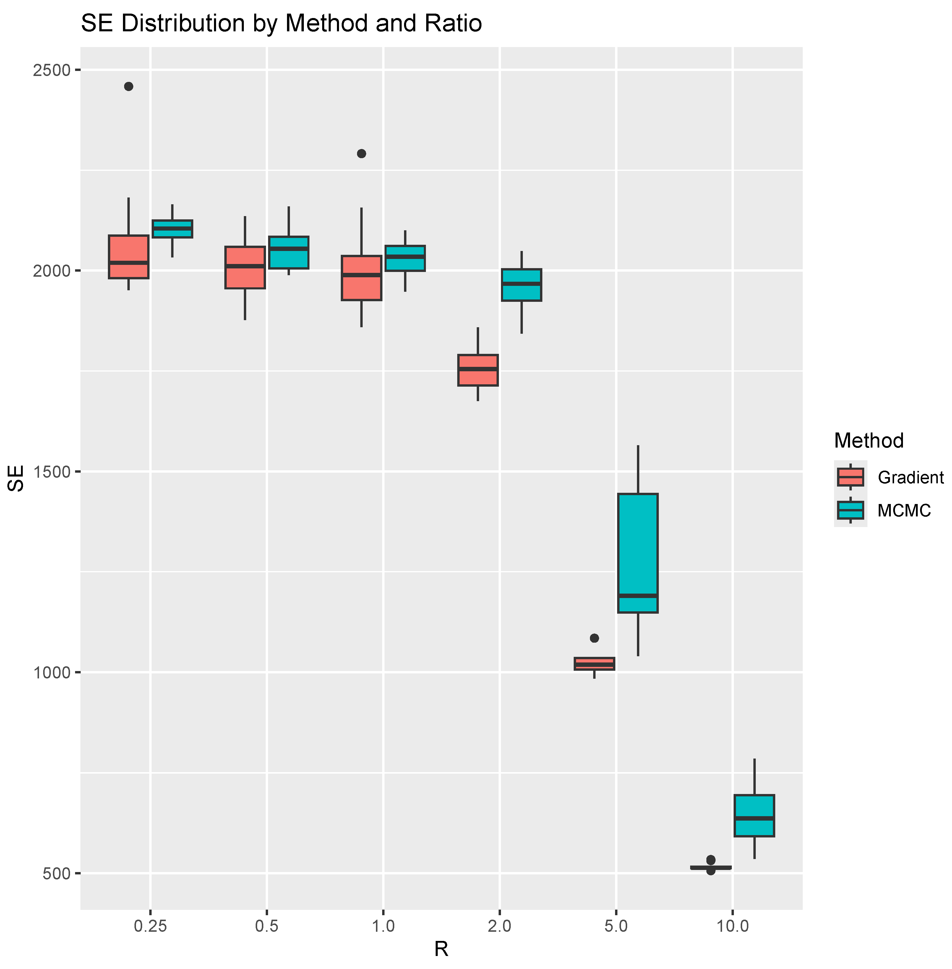
In this experiment, we simulate 1000 trees for each valuee of R = 0.25, 0.5, 1.0, 2.0, 5.0, 10.0. We run 100 iterations of both the MCMC method and our projected gradient method. To account for variability in performance, we repeat both methods 10 times for each R. For each run, we compute the sum of tropical distances $d_{\mathrm{tr}}$ between the observed trees and their projections onto the estimated tropical polytope. This sum, representing the total “magnitude of errors” (SE) in terms of $d_{\mathrm{tr}}$), corresponds to the estimated optimal value of the linear programming problem in Problem 1. The results are shown in Figure 2. For the learning rate schedule, we start with $\lambda =0.001$ and multiply it by $0.999$ at each iteration. Note that this learning rate has not been optimized. Therefore, investigating an optimal learning rates remains a direction for future work. As for the stopping criterion, we terminate the algorithm when the preset maximum number of iterations is reached. Each iteration has time complecity $O\left(m^{2}n\right)$, where n is the sample size.

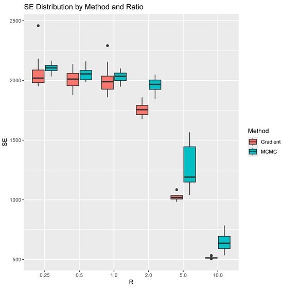
Figure 2. Side-by-side boxplots for the SE for each method and ratio. We repeat computation 10 times for each ratio and method.

5.2. Empirical Dataset

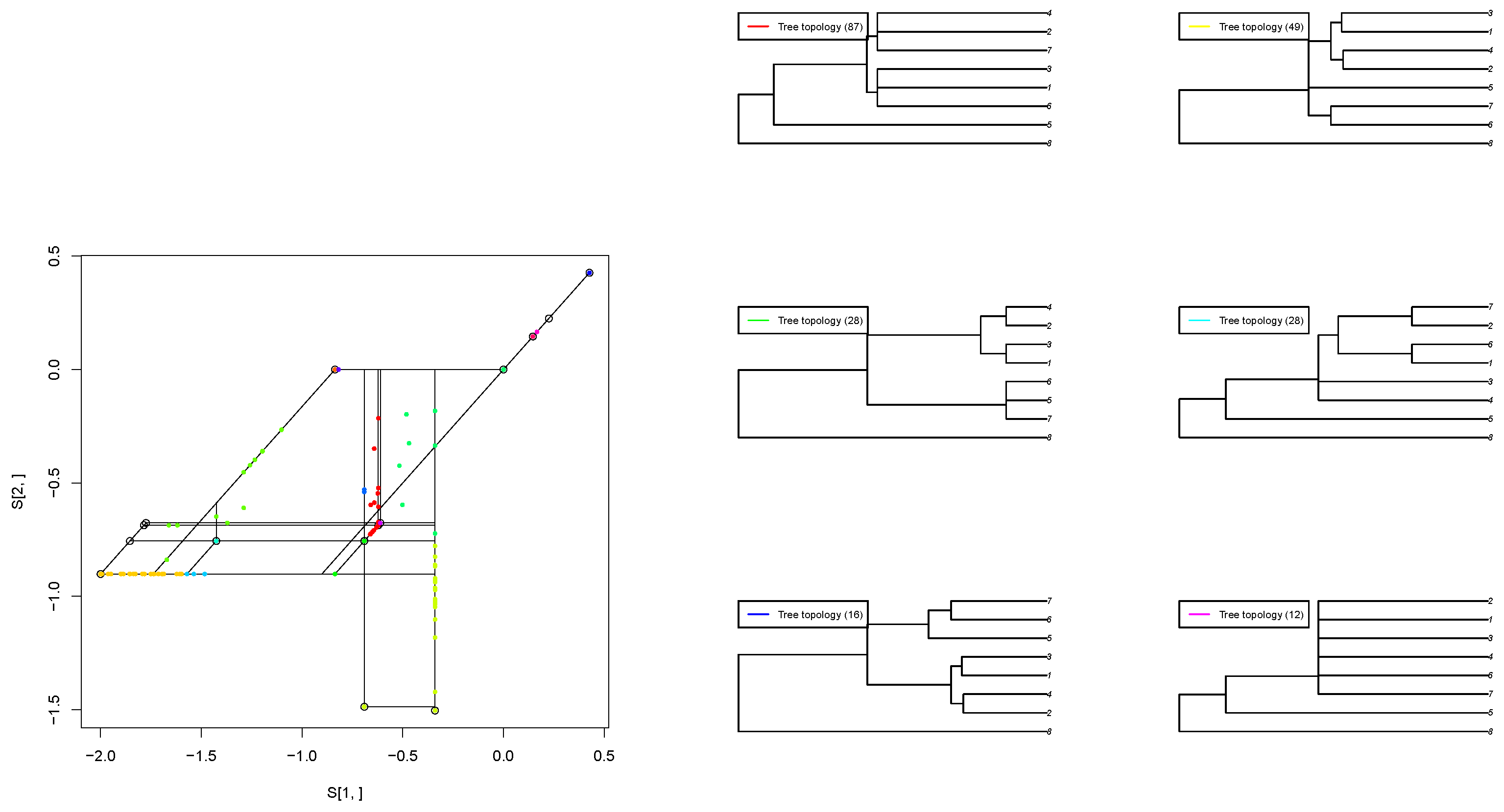
We apply our projected gradient method to estimate the best-fit tropical polytope for an empirical dataset consisting of 268 orthologous sequences from eight protozoa species, as presented in [5]. This dataset contains gene trees reconstructed from the following sequences: Babesia bovis (Bb), Cryptosporidium parvum (Cp), Eimeria tenella (Et) [15], Plasmodium falciparum (Pf) [11], Plasmodium vivax (Pv), Theileria annulata (Ta), and Toxoplasma gondii (Tg). The outgroup is a free-living ciliate, Tetrahymena thermophila (Tt) (Figure 3).

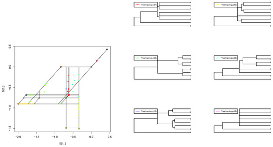
Figure 3. (Left): Estimated second-order tropical principal polytope. (Right): Each color represents a tree topology. The number inside each bracket is the frequency of the tree topology. 1 presents “Pv”, 2 represents “Pf”, 3 represents “Tg”, 4 represents “Et”, 5 represents “Cp”, 6 represents “Ta”, 7 represents “Bb” and 8 represents “Tt”.

In order to run this experiment, we used a Mac Pro laptop (Apple Inc., Cupertino, CA, USA) with Apple M4 Max and 128 GB memory. We implemented our projected gradient method using R.

We set the maximum number of iterations to 100 for our projected gradient method, and to 1000 for the MCMC method. For the learning rate schedule, we initialize $\lambda =0.01$ and multiply it by $0.999$ at each iteration. Note that the learning rate and scheduling have not been optimized. Using the projected gradient descent to estimate the tropical principal polytope on this dataset takes $6.82$ s, resulting in an estimated optimal value of $360.8589$ for the optimization problem in Problem 1. In comparison, the Markov Chain Monte Carlo (MCMC) method implemented via the TML package [6] yields an estimated optimal value of $397.6459$, with a computational time of $54.70$ s over 1000 iterations.

6. Conclusions

In this work, we introduce a novel method to approximate the best-fit tropical polytope that explains a sample of gene trees. We show that our gradient method effectively reduces the objective function when an appropriate learning rate is used. Computational experiments show that this method achieves a lower sum of tropical distances between observations and their projections onto the estimated best-fit tropical polytope, compared to the MCMC approach proposed by Page et al. [13]. Although we implement a decreasing learning rate in our experiments, the optimal learning rate schedule for this problem remains an open question.

We implement our method in R and the source code is available at http://polytopes.net/Tropical_Gradient2.zip (accessed on 15 May 2025).

References

- Buneman, P. A note on the metric properties of trees. J. Comb. Theory Ser. B 1974, 17, 48–50. [Google Scholar] [CrossRef]
- Ardila, F.; Klivans, C.J. The Bergman Complex of a Matroid and Phylogenetic Trees. J. Comb. Theory Ser. B 2006, 96, 38–49. [Google Scholar] [CrossRef]
- Yoshida, R.; Zhang, L.; Zhang, X. Tropical Principal Component Analysis and its Application to Phylogenetics. Bull. Math. Biol. 2019, 81, 568–597. [Google Scholar] [CrossRef] [PubMed]
- Talbut, R.; Monod, A. Tropical Gradient Descent. arXiv 2024, arXiv:2405.19551. [Google Scholar] [CrossRef]
- Kuo, C.; Wares, J.P.; Kissinger, J.C. The Apicomplexan Whole-Genome Phylogeny: An Analysis of Incongruence among Gene Trees. Mol. Biol. Evol. 2008, 25, 2689–2698. [Google Scholar] [CrossRef] [PubMed]
- Barnhill, D.; Yoshida, R.; Aliatimis, G.; Miura, K. Tropical geometric tools for machine learning: The TML package. J. Softw. Algebra Geom. 2024, 14, 133–174. [Google Scholar] [CrossRef]
- Maclagan, D.; Sturmfels, B. Introduction to Tropical Geometry; Graduate Studies in Mathematics; American Mathematical Society: Providence, RI, USA, 2015; Volume 161. [Google Scholar]
- Joswig, M. Essentials of Tropical Combinatorics; Springer: New York, NY, USA, 2021. [Google Scholar]
- Feichtner, E.M. Complexes of trees and nested set complexes. Pac. J. Math. 2004, 227, 271–286. [Google Scholar] [CrossRef]
- Ardila, F. Subdominant Matroid Ultrametrics. Ann. Comb. 2005, 8, 379–389. [Google Scholar] [CrossRef]
- Jaggi, M.; Katz, G.; Wagner, U. New results in tropical discrete geometry. Preprint 2008. Available online: https://api.semanticscholar.org/CorpusID:14825187 (accessed on 14 April 2025).
- Gascuel, O.; McKenzie, A. Performance analysis of hierarchical clustering algorithms. J. Classif. 2004, 21, 3–18. [Google Scholar] [CrossRef]
- Page, R.; Yoshida, R.; Zhang, L. Tropical principal component analysis on the space of phylogenetic trees. Bioinformatics 2020, 36, 4590–4598. [Google Scholar] [CrossRef] [PubMed]
- Barnhill, D.; Sabol, J.; Yoshida, R.; Miura, K. Tropical Fermat-Weber Polytropes. arXiv 2024, arXiv:2402.14287. [Google Scholar] [CrossRef]
- Maddison, W.P.; Maddison, D. Mesquite: A Modular System for Evolutionary Analysis. Version 2.72. 2009. Available online: http://mesquiteproject.org (accessed on 11 August 2016).
Disclaimer/Publisher’s Note: The statements, opinions and data contained in all publications are solely those of the individual author(s) and contributor(s) and not of MDPI and/or the editor(s). MDPI and/or the editor(s) disclaim responsibility for any injury to people or property resulting from any ideas, methods, instructions or products referred to in the content. |
© 2025 by the author. Licensee MDPI, Basel, Switzerland. This article is an open access article distributed under the terms and conditions of the Creative Commons Attribution (CC BY) license (https://creativecommons.org/licenses/by/4.0/).