Optimizing Sustainable Supply Chains: An Analysis of Quantity-Discount Pricing Strategies Under Carbon Cap-and-Trade Regulations

Abstract

This study investigates two pricing strategies within a vendor-buyer supply chain system under cap-and-trade regulation, emphasizing demand sensitivity to market price and green technology investment. The findings reveal that quantity discounts significantly enhance profitability across the supply chain by encouraging buyers to place larger orders, thereby benefiting vendors, buyers, and end consumers. A novel profit-sharing parameter is introduced to foster sustainable and mutually beneficial relationships between supply chain participants. A search algorithm is developed to determine the optimal solutions by using the profit-sharing mechanisms. The analysis yields three key insights: first, a critical cap threshold is identified, enabling supply chain participants to make informed strategic decisions based on the value of the cap; second, another critical cap threshold is derived to assist governments in setting feasible emission limits that incentivize vendors to invest in green technology—caps below this threshold may discourage such investments; third, a reasonable return on investment (ROI) benchmark is established to guide vendors in adopting effective green technology strategies. Numerical examples and sensitivity analyses are conducted to illustrate the theoretical framework and validate the findings.

1. Introduction

The rising importance of environmental issues, governmental regulations through imposing tariffs, and social responsibility has led to increased research attention on sustainable supply chain management. Sustainability in supply chain management has emerged as a critical focus for businesses worldwide, driven by increasing environmental concerns and societal expectations. A sustainable supply chain integrates environmental, social, and governance (ESG) principles into operational practices to minimize ecological harm while promoting social equity and economic viability. Its overarching goal is to reduce the negative environmental impact of supply chains while enhancing social welfare and maintaining profitability.

The importance of this study lies in addressing one of the most pressing global challenges: carbon emissions. Carbon emissions are nearly irreversible and have far-reaching consequences for climate change, biodiversity loss, and public health. Governments worldwide are implementing policies such as subsidies, penalties, and cap-and-trade regulations to curb emissions. However, achieving meaningful reductions requires coordinated efforts across supply chains involving vendors, buyers, and consumers. This study contributes to this effort by exploring how pricing strategies can align economic incentives with environmental goals through green technology investments and carbon emission reductions.

The complexity of carbon reduction initiatives stems from several factors: government intervention through carbon pricing mechanisms; coordination among supply chain participants; investments in green technologies; consumer awareness of ESG concerns; and willingness to pay higher prices for environmentally sustainable products. These challenges necessitate innovative approaches that balance profitability with sustainability.

The high-tech industry serves as a compelling example of these dynamics. For instance, producing an iPhone X generates approximately 80 kg of carbon emissions. In Sweden, where carbon taxes are among the highest globally, Apple could face taxation exceeding USD 10 per unit—a cost that could amount to approximately USD 2 billion annually if applied globally. To address these challenges, Apple has implemented significant sustainability measures. As outlined in its 2020 Environmental Progress Report, Apple achieved 100% carbon neutrality across its operations by 2019 through initiatives such as renewable energy adoption and collaboration with over 100 supply chain partners to transition to sustainable practices. Furthermore, Apple has committed to ensuring that every device sold will have a net-zero climate impact by 2030. This case study highlights the broader implications for global industries: prioritizing environmental sustainability can yield substantial benefits for companies while addressing critical societal concerns.

Literature Review

In the era of environmental concerns and trade protection through imposing tariffs, Daryanto et al. [1] explored low carbon supply chain coordination for imperfect quality deteriorating items. Hua et al. [2] focused on deriving an economic lot size by incorporating carbon footprints into inventory management, aiming to minimize total costs under constant demand conditions. Dwicahyani et al. [3] introduced a supply chain inventory system that includes a warehouse and a distributor, addressing environmental and remanufacturing capacity constraints. Their analysis indicated that while the system may increase waste and carbon emissions, it can reduce energy consumption. They also noted that increasing the collection of returned products could lower the total joint cost. Ghosh et al. [4] examined the optimization of production batch sizes under conditions of stochastic market demand, carbon emission caps, and partial stock outs, taking into account significant emission sources like production, storage, and transportation. Tiwari et al. [5] developed a pricing and inventory model that accounts for housing, transportation, imperfect quality, and related carbon emission costs. Yang and Chen [6] explored the use of green quality costs and sales revenue sharing as mechanisms to achieve Pareto optimality in supply chain operations. Bai et al. [7] suggested that governmental subsidies for carbon emission reduction could incentivize manufacturers to invest in green technology facilities.

Turki et al. [8] investigated the differences between new and remanufactured products, considering factors such as random machine failures, carbon constraints, and random demand. Their study analyzed the effects of carbon emission caps, carbon trading prices, and the proportion of recycled materials on carbon emissions. Chelly et al. [9] contributed to the field of operations management (OM) by focusing on low-carbon supply chain management (LCSCM) within the broader context of green supply chain management (GSCM). Their review highlighted supply chain management research specifically aimed at reducing carbon emissions and managing associated constraints. Yu et al. [10] established a closed-loop inventory model involving a manufacturer and a retailer, with both return and demand rates being sensitive to price. Their study aimed to optimize sales prices, return prices, batch sizes for new and returned components, and production quantities delivered to retailers. Taleizadeh et al. [11] considered carbon reduction, return policies, and quality improvement as key factors, examining technology investment, trading, and capping strategies to reduce carbon emissions in forward logistics. They also studied hybrid remanufacturing of imperfect quality products under technology licensing in reverse logistics, assessing the impact of remanufacturing on carbon emission reduction, quality enhancement, and overall supply chain efficiency.

Integrating environmental protection into traditional supply chain design through the collection and reuse of used products is a primary goal of closed-loop systems, which encompass both forward and reverse supply chains. A study by Nahr et al. [12] developed a bi-objective, multi-period, multi-product closed supply chain network, incorporating environmental considerations, discount strategies, and system uncertainties. Entezaminia et al. [13] focused on developing cost-effective and environmentally friendly control policies for companies implementing green investments, analyzing the impact of cost and system parameters on these strategies. Taleizadeh et al. [14] also explored a vendor-managed inventory system, where suppliers make replenishment decisions at the buyer’s location to enhance supply chain coordination, considering partial stock outs and limited storage capacity. Ramandi and Bafruei [15] examined the reduction of greenhouse gas emissions in a two-tier supply chain with one supplier and one retailer under government policies, focusing on emissions from transportation. Roy and Sana [16] investigated strategies for simultaneously reducing lead time and setup costs in a two-stage supply chain model under trade credit financing, considering the impact of variable production rates and batch sizes on delivery times. Rout et al. [17] developed a sustainable supply chain inventory management (SSCIM) model using an integrated approach with a single supplier and multiple buyers, addressing item spoilage and imperfect production. Jiang and Jiang [18] analyzed cooperative and competitive dynamics between original equipment manufacturers (OEMs) and contract manufacturers (CMs) concerning green investments. Hoque [19] proposed a single-manufacturer multi-retailer integration model, incorporating carbon neutrality mechanisms and imperfect remanufacturing processes. Heydari et al. [20] analyzed supply chain coordination between a manufacturer and a buyer under demand conditions sensitive to price and green quality, applying a hybrid strategy combining green cost and revenue sharing to achieve channel coordination. Recently, Sarkar and Bhuniya [21] developed a model focusing on flexible manufacturing–remanufacturing with green investments under variable demand. Their work emphasizes the integration of service facilities to enhance customer satisfaction and sustainability. Sarkar and Guchhait [22] examined the impact of information asymmetry on green supply chains, incorporating cap-and-trade policies, service levels, and vendor-managed inventory strategies. They utilized RFID technology to mitigate asymmetry and improve coordination. Guchhait et al. [23] proposed an extended MRP framework within hybrid energy-enabled smart production systems. Their model integrates renewable energy sources and reverse logistics, demonstrating cost savings and enhanced sustainability. Guchhait and Sarkar [24] analyzed the economic implications of outsourcing logistics to 4PL providers in flexible production systems, particularly for deteriorating products. Their findings suggest significant cost reductions and improved efficiency.

Table 1. Comparison between the proposed work and previous studies.

Authors (Year)	Sustainable Supply Chains	Carbon Reduction	Pricing Strategy	Profit/Cost Negotiation Mechanism
Daryanto et al. (2019) [1]	Yes	Yes	No	No
Hua et al. (2011) [2]	No	Yes	No	No
Dwicahyani et al. (2017) [3]	Yes	No	No	No
Ghosh et al. (2017) [4]	No	Yes	No	No
Tiwari et al. (2018) [5]	No	Yes	Yes
Yang and Chen (2018) [6]	Yes	No	No	Yes
Bai et al. (2018) [7]	No	Yes	No	Yes
Turki et al. (2018) [8]	No	Yes	No	No
Chelly et al. (2019) [9]	Yes	Yes	No	No
Yu et al. (2019) [10]	Yes	No	Yes	No
Taleizadeh et al. (2019) [11]	Yes	Yes	No	No
Nahr et al. (2020) [12]	Yes	No	Yes	No
Entezaminia et al. (2020) [13]	Yes	No	No	No
Taleizadeh et al. (2020) [14]	Yes	No	No	No
Ramandi and Bafruei (2020) [15]	No	Yes	No	No
Roy and Sana (2021) [16]	No	No	No	Yes
Rout et al. (2021) [17]	Yes	No	No	No
Jiang et al. (2021) [18]	Yes	No	No	No
Hoque, M. (2021) [19]	Yes	Yes	No	No
Heydari et al. (2021) [20]	Yes	No	Yes	Yes
Sarkar and Bhuniya (2022) [22]	Yes	No	Yes	Yes
Sarkar and Guchhait (2023) [23]	Yes	No	Yes	Yes
Guchhait et al. (2024) [24]	Yes	No	Yes	Yes
Guchhait and Sarkar (2025) [25]	Yes	No	Yes	Yes
Proposed model	Yes	Yes	Yes	Yes

shows the differences between this study and existing studies. Our study can fill the research gap for sustainable supply chains inside thoroughly regarding negotiation mechanism.

Environmental issues must be addressed and implemented over the long term because the implementation of environmental protection is crucial to whether a company can operate sustainably and whether society can survive healthily forever. Pricing strategy is related to the competitiveness of enterprises in the market. The above two problem characteristics are very important for today’s business operations.

This study considered the setup, holding, green facility cost, and penalty cost when the demand is sensitive to price and green technology level. The goals are the improvements in manufacturing processes, energy efficiency, product design optimization, recycling initiatives, and pollution reduction. By examining pricing strategies within a sustainable supply chain framework under cap-and-trade regulation, this study provides valuable insights into how businesses can align their operations with environmental objectives while maintaining economic competitiveness.

2. Modelling

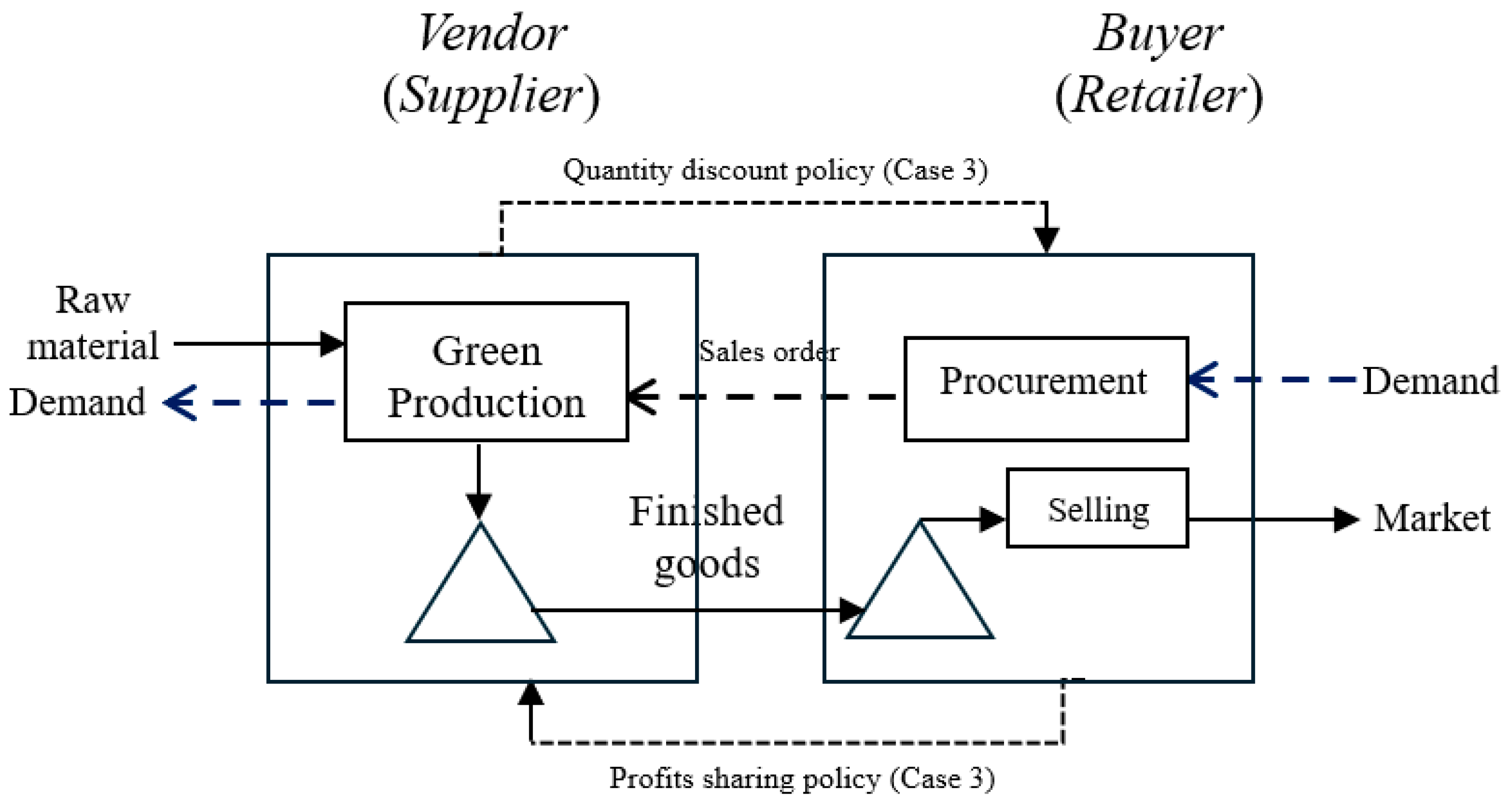
This study developed a quantity-discount pricing strategy model with a market price and technology level of carbon emission reduction sensitive demand. Take the famous retailer, Walmart, as an example. We compared the effects of the three cases when facing a leader of the supply chain. Figure 1 shows how the two parties behave in a two-echelon supply chain in our study.

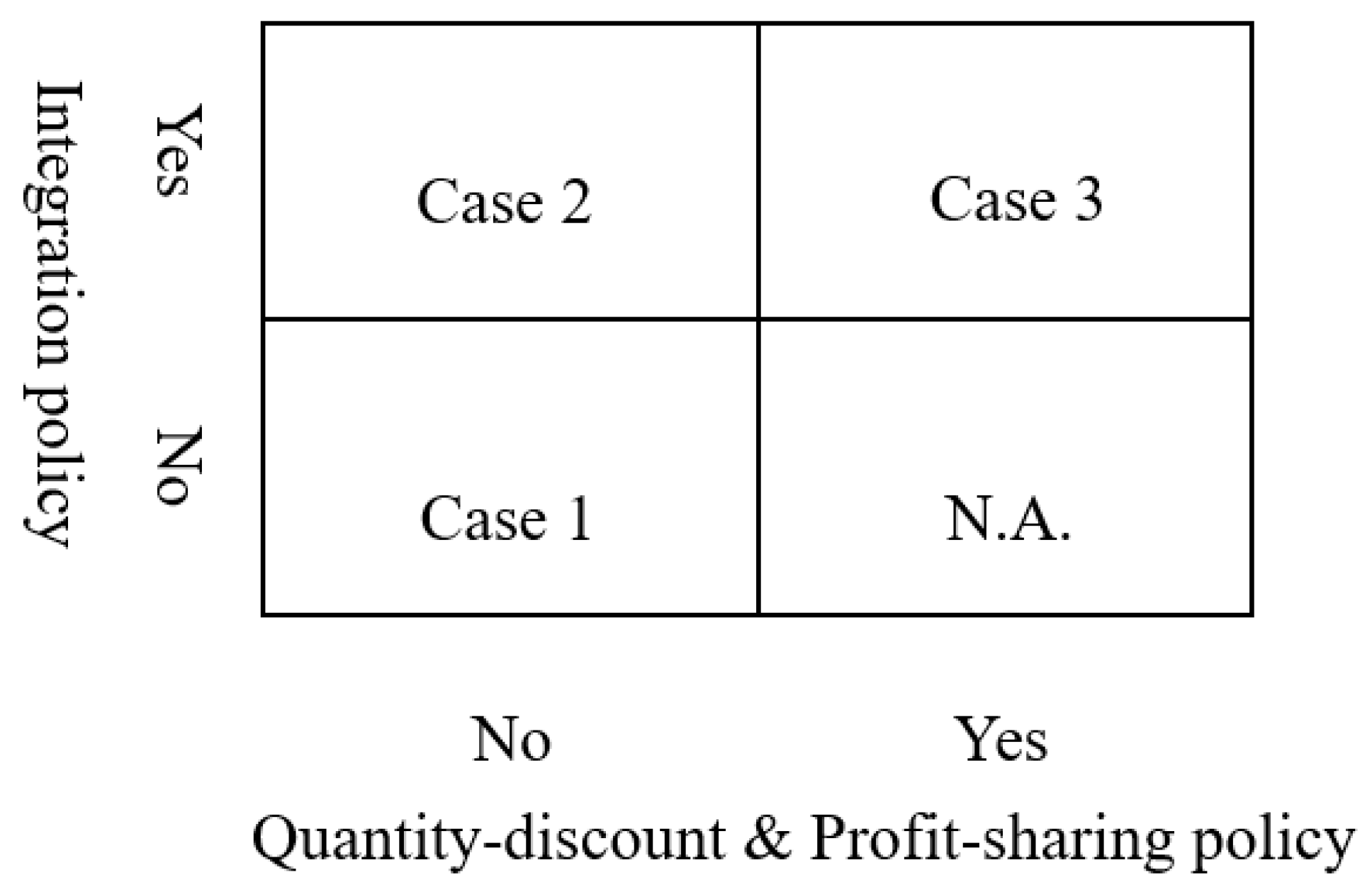
The scenario matrix of our study is shown in Figure 2. Case 1 is an equal strength case in point when the supplier is also very powerful, and they will make their own buying and selling decisions. Case 2 is an example of an unequal relationship between vendor and buyer, when Walmart’s suppliers have a high dependence on Walmart. Suppliers will choose to integrate into Walmart’s system to seek opportunities for stable development of their own businesses. So, the vendor will cooperate with the buyer to make decisions. In the example of Case 3, in addition to being highly dependent on Walmart, the supplier may have competitors in the Walmart system. Therefore, in addition to complying with the integration, the supplier also provides discounts, combined with Walmart’s profit-sharing mechanism, to create a win-win opportunity for both buyers and sellers. To ensure mutually beneficial strategy, in Case 3, a negotiation factor is incorporated to enable profit sharing between both parties.

The mathematical model developed in this paper is based on the following assumptions:

(a)

There is one vendor and one buyer.

(b)

The vendor’s (or manufacturer’s) replenishment rate is finite.

(c)

The demand rate is sensitive to market price and technology level of carbon emission reduction.

(d)

All unit quantity discounts are considered.

(e)

The vendor is fully responsible for carbon emission reduction.

(f)

The players have complete knowledge of each other’s information.

Three cases are discussed: the first case considers a buyer’s market, where the buyer prioritizes maximizing their profit. The second case considers the integration to maximize vendor-buyer profit. The third case considers integration and quantity discount.

The decision variables are as follows:

S: The technology level of carbon emission reduction

P_m: Market price

T_b: The replenishment period for the buyer

N: Number of replenishments per cycle for the retailer

P_b: Buyer’s unit purchase cost from the vendor in Case 3 (constant in Cases 1 and 2)

The buyer’s other related parameters are:

d: Market demand rate

d₀: Potential market demand rate

d₁: Technology level sensitive coefficient of carbon emission reduction on market demand

d₂: Price-sensitive coefficient on market demand

C_b: Setup cost per replenishment

F_b: Holding cost per dollar per unit time

The vendor’s related parameters are:

C_v: Setup cost per production cycle

C_vb: Fixed cost to process each replenishment to the buyer

F_v: Holding cost per dollar per unit time

P_v: Unit purchase cost

$g$: Production rate

C: Cap (or called quota) of carbon emission regulated by the government

C_p: Unit price per carbon emission that can be bought (or sold) from an organization when the manufacturer’s carbon emission exceeds (or is less than) the cap C

${\displaystyle \frac{1}{2}}\eta S^2$: Facility cost of green technology, where $\eta$ is the influence coefficient

$a-bS$: Carbon emission for each one produced product, where $a>bS$. a: base carbon emission per unit product when the carbon emission reduction technology level is zero, a > 0; and b: influence coefficient of emission reduction technology on reducing emissions, b > 0.

Other related parameters:

$\mathsf{\Phi }$: Negotiation factor between vendor and buyer for sharing extra profit

TP_b: Buyer’s total profit, considering net sales revenue, setup cost, and holding cost

TP_v: Vendor’s total profit, considering net sales revenue, setup cost, and holding cost

TP: Total profit, considering net sales revenue, setup cost, and holding cost, where $TP={TP}_b+{TP}_v$

${TC}_{vg}$: Green cost, including facility cost and the penalty cost (or subsidy) with government cap-and-trade regulation, ${TC}_{vg}\ge 0 or {TC}_{vg}\le 0$

${TP}_v^{\#}$: ${TP}_v^{\#}={TP}_v-{TC}_{vg}$

TP^#: Total profit considering net sales revenue, setup cost, holding cost, and green cost, where ${TP}^{\#}={TP}_v^{\#}+{TP}_b$.

When the demand is sensitive to market price and technology level of carbon emission reduction, it is assumed as follows:

$$d=d_0+d_{1}S-d_2{P}_m$$

(1)

The buyer’s total profit is expressed as:

$${TP}_b(P_m,S,T_b)=\left(P_m-P_b\right)d-{\displaystyle \frac{C_b}{T_b}}-{\displaystyle \frac{1}{2}}{P}_{b}d{T}_b{F}_b$$

(2)

On the right side of Equation (2), the first item represents net sales revenue, the second item represents setup cost, and the last item represents holding cost. The vendor’s (or manufacturer’s) total profit can be expressed as:

$${TP}_v\left(P_m,S,T_b,N\right)=\left(P_b-P_v\right)d-{\displaystyle \frac{C_v+N{C}_{vb}}{N{T}_b}}-{\displaystyle \frac{1}{2}}d{T}_b\left[\left(N-1\right)\left(1-{\displaystyle \frac{d}{g}}\right)+{\displaystyle \frac{d}{g}}\right]P_v{F}_v$$

(3)

On the right side of Equation (3), the first item represents net sales revenue, the second item represents the setup cost, and the third item represents the holding cost. The expression ${\displaystyle \frac{1}{2}}d{T}_b[\left(N-1\right)\left(1-{\displaystyle \frac{d}{g}}\right)+{\displaystyle \frac{d}{g}}]$ represents the average inventory level for the vendor when the replenishment rate is constant. The sum of Equations (2) and (3) can be expressed as:

$$TP\left(P_m,S,T_b,N\right)={TP}_b\left(P_m,S,T_b\right)+{TP}_v\left(P_m,S,T_b,N\right)$$

(4)

Generally, the pressure of carbon emission reduction is placed on the manufacturer (or vendor) instead of the retailer (or buyer). The vendor’s green cost and total profit are expressed as:

$${TC}_{vg}(S,P_m)={\displaystyle \frac{1}{2}}\eta S^2+C_p[\left(a-bS\right)d-C]$$

(5)

where $a>0,b>0,a>bS$

$${TP}_v^{\#}\left(P_m,S,T_b,N\right)={TP}_v\left(P_m,S,T_b,N\right)-{TC}_{vg}(S,P_m)$$

(6)

On the right-hand side of Equation (5), the first item represents the cost of facility investment in carbon emission reduction, and the second item represents the loss (or earn) when the actual carbon emission exceeds (or falls short of) the cap of carbon emission. The sum of Equations (2) and (6) are written as:

$${TP}^{\#}\left(P_m,S,T_b,N\right)={TP}_b\left(P_m,S,T_b\right)+{TP}_v^{\#}\left(P_m,S,T_b,N\right)$$

(7)

In Equation (7), there are four decision variables. Within the whole system of the vendor and buyer, including the green cost of carbon emission reduction, the problem is:

$$Maximize {TP}^{\#}\left(P_m,S,T_b,N\right)$$

(8)

Subject to $S\ge 0,P_m\ge 0,T_b\ge 0,N\ge 0$.

Let $S^{*}$ be the optimal solution of (8). After substituting $S=S^{*}$ and demand d in Equation (1) into Equations (2) and (3), ${TP}_b$ and ${TP}_v$ are expressed as:

$${TP}_b\left(P_m,T_b\right)=\left(P_m-P_b\right)\left(d_0+d_1{S}^{*}-d_2{P}_m\right)-{\displaystyle \frac{C_b}{T_b}}-{\displaystyle \frac{1}{2}}{P}_b(d_0+d_1{S}^{*}-d_2{P}_m)T_b{F}_b$$

(9)

$$\begin{array}{ll}{TP}_v^{\#}\left(P_m,T_b,N\right)& =\left(P_b-P_v\right)\left(d_0+d_1{S}^{*}-d_2{P}_m\right)-{\displaystyle \frac{C_v+N{C}_{vb}}{N{T}_b}}\\ & -{\displaystyle \frac{1}{2}}d{T}_b\left[\left(N-1\right)\left(1-{\displaystyle \frac{\left(d_0+d_1{S}^{*}-d_2{P}_m\right)}{g}}\right)+{\displaystyle \frac{\left(d_0+d_1{S}^{*}-d_2{P}_m\right)}{g}}\right]P_v{F}_v-{TC}_{vg}(S^{*},P_m)\end{array}$$

(10)

Case 1: Considering a buyer’s market without a quantity discount

In this case, the vendor offers a fixed price to the buyer and the buyer decides the values of P_m and T_b in Equation (9). Since the value of S (i.e., green technology level) in Equation (9) is related to the green cost of carbon emission reduction, it is reasonable for the vendor to set the value of $S$ to be equal to $S^{*}$.

Case 2: Considering vendor-buyer integration without quantity discount

In this case, the vendor and buyer make the decision in Equation (8) simultaneously.

Case 3: Considering integration and quantity discount

The vendor offered a discount-price $P_b$ to the buyer. In this case, there are five decision variables: $P_m$, S, $T_b$, N and $P_b$ in Equation (8). Let the optimum values of ${TP}_b$ and ${TP}_v$ $(or {TP}_v^{\#})$ in Case 1 be expressed as ${TP}_{b1}$ and ${TP}_{v1}$ $(or {TP}_{v1}^{\#})$, respectively.

Two pricing strategies for sharing the extra profit are discussed as follows:

Strategy I: Sharing the extra profit from net sales revenue, setup cost, and holding cost. The characteristic of Strategy I is when the discount price remains stable.

Strategy II: Sharing the extra profit from net sales revenue, setup cost, holding cost, and green cost. The green cost may be positive or negative depending on whether ${\displaystyle \frac{1}{2}}\eta S^2>C_p[\left(a-bS\right)d-C]$ or ${\displaystyle \frac{1}{2}}\eta S^2<C_p\left[\left(a-bS\right)d-C\right],$ respectively. The characteristic of Strategy II is that the discount price adjusts according to the government’s carbon emission cap.

The extra total profit for the buyer (or the vendor) in Case 3 is defined as the difference in total profit between Case 3 and Case 1. It is written as:

$$∆{TP}_b={TP}_b-{TP}_{b1}$$

(11)

and

$$∆{TP}_v={TP}_v-{TP}_{v1}(or {∆TP}_v^{\#}={TP}_v^{\#}-{TP}_{v1}^{\#})$$

(12)

A key parameter in negotiating the profit share between the vendor and the buyer, $\mathsf{\Phi }$, is defined as:

$$(∆{TP}_v)=\mathsf{\Phi }(∆{TP}_b) or \left({∆TP}_v^{\#}\right)=\mathsf{\Phi }\left({∆TP}_b\right)$$

(13)

If $\mathsf{\Phi }=1$, it means the vendor’s extra total profit is equal to the buyer’s extra total profit. If $\mathsf{\Phi }=100$ (or $\mathsf{\Phi }=10)$, the vendor’s profit is more than 100 times (or 10 times) compared to the buyer’s extra total profit. A constrained problem in Case 3 can be rewritten as:

$$Maximize {TP}^{\#}\left(P_m,{S,T}_b,P_b,N\right)$$

(14)

$$\mathit{Subject}\mathit{to} (∆{TP}_v)=\mathsf{\Phi }(∆{TP}_b)$$

$$or\left({∆TP}_v^{\#}\right)=\mathsf{\Phi }\left({∆TP}_b\right)$$

3. Solution Procedure

Case 1:

The buyer’s total profit is optimized first, followed by the vendor’s total profit.

Step 1: By taking the first derivative of ${TP}_b\left(P_m,T_b\right)$ with respect to $P_m,T_b$ setting to zero simultaneously, the value of $P_m,T_b$ is determined.

$${\displaystyle \frac{\mathsf{\partial }{TP}_b\left(P_m,T_b\right)}{\mathsf{\partial }{P}_m}}=0$$

(15)

$${\displaystyle \frac{\mathsf{\partial }{TP}_b\left(P_m,T_b\right)}{\mathsf{\partial }{T}_b}}=0$$

(16)

Step 2: The optimal solution of $N^{\zeta }$, denoted as $N^{\zeta *}$, must satisfy the following conditions:

$${TP}_v^{\#}(N^{\zeta *}-1)\le {TP}_v^{\#}\left(N^{\zeta *}\right)\ge {TP}_v^{\#}(N^{\zeta *}+1)$$

(17)

Case 2:

The total profit in Equation (8) is optimized. For a fixed value of N (denoted $N^{\zeta }$), the following conditions must be satisfied simultaneously.

Step 1: By taking the first derivative of ${TP}^{\#}\left(P_m,S,T_b,N\right)$ with respect to $P_m,S,T_b, N$ setting to zero simultaneously, the value of $P_m,S,T_b, N$ is determined.

$${\displaystyle \frac{\mathsf{\partial }{TP}^{\#}(P_m,{S,T}_b,N^{\zeta })}{\mathsf{\partial }{P}_m}}=0$$

(18)

$${\displaystyle \frac{\mathsf{\partial }{TP}^{\#}(P_m,S,T_b,N^{\zeta })}{\mathsf{\partial }S}}=0$$

(19)

$${\displaystyle \frac{\mathsf{\partial }{TP}^{\#}(P_m,S,T_b,N^{\zeta })}{\mathsf{\partial }{T}_b}}=0$$

(20)

Step 2: The optimal solution of $N^{\zeta }$ must satisfy the following conditions:

$${TP}^{\#}(N^{\zeta }-1)\le {TP}^{\#}\left(N^{\zeta }\right)\ge {TP}^{\#}(N^{\zeta }+1)$$

(21)

Case 3:

The first step is to derive $P_b$ from Equation (13), where $P_b$ is expressed as $P_b(P_m,{S,T}_b,N)$. For a fixed value of N (denoted as $N^{\zeta }$), the optimal solution in Equation (14) must simultaneously satisfy the following conditions:

Step 1: By taking the first derivative of ${TP}^{\#}(P_m,S,T_b,P_b,N)$ with respect to $P_m,S,T_b,P_b,N$ setting to zero simultaneously, the value of $P_m,S,T_b,P_b,N$ is determined.

$${\displaystyle \frac{\mathsf{\partial }{TP}^{\#}(P_m,S,T_b,P_b(P_m,T_b,N^{\zeta }),N^{\zeta })}{\mathsf{\partial }{P}_m}}=0$$

(22)

$${\displaystyle \frac{\mathsf{\partial }{TP}^{\#}(P_m,S,T_b,P_b(P_m,T_b,N^{\zeta }),N^{\zeta })}{\mathsf{\partial }S}}=0$$

(23)

$${\displaystyle \frac{\mathsf{\partial }{TP}^{\#}(P_m,S,T_b,P_b\left(P_m,T_b,N^{\zeta }\right),N^{\zeta })}{\mathsf{\partial }{T}_b}}=0$$

(24)

Step 2: The optimal solution of $N^{\zeta }$ must satisfy the following conditions:

$${TP}^{\#}(N^{\zeta }-1)\le {TP}^{\#}\left(N^{\zeta }\right)\ge {TP}^{\#}(N^{\zeta }+1)$$

(25)

4. Numerical Example and Sensitivity Analysis

4.1. Numerical Example for Three Cases

In this study, the following example data illustrate the proposed approach. They are offered by Yiming Co. Ltd., Taiwan, (Taiwan, China) which belongs to A&I Group. The factory produces consumer goods and utensils through plastic injection molding and metal extrusion molding and sells to large-scale hypermarkets.

The buyer-related parameters are $C_b$ = 100; $F_b$ = 0.3; $P_b$ = 35 for Cases 1 and 2. The vendor-related parameters are: $C_v$ = 6000; $C_{vb}$ = 100; $F_v$ = 0.2; $P_v$ = 20; g = 30000. The parameters related to green technology are C = 300,000, $C_p$ = 0.5. $\eta$ = 1.5. a = 425. b = 1.1. The demand parameters: $d_0$ = 3000; $d_1$ = 0.1; $d_2$ = 35. The negotiation factor:$\mathsf{\Phi }$ = 100, 10, 1, 0.1, and 0.01. By applying the above solution procedure, the results for Cases 1, 2, and 3 are presented in

Table 2. The optimum solution in various cases.

Case i	Case 1	Case 2	Case 3
			$\mathit{S}\mathit{t}\mathit{r}\mathit{a}\mathit{t}\mathit{e}\mathit{g}\mathit{y}\mathit{I}$ $(∆{\mathit{T}\mathit{P}}_{\mathit{v}})=(∆{\mathit{T}\mathit{P}}_{\mathit{b}})$	$\mathit{S}\mathit{t}\mathit{r}\mathit{a}\mathit{t}\mathit{e}\mathit{g}\mathit{y}\mathit{I}\mathit{I}$ $\left({∆\mathit{T}\mathit{P}}_{\mathit{v}}^{\#}\right)=\left({∆\mathit{T}\mathit{P}}_{\mathit{b}}\right)$
N	13	7	7	7
S	379.24	379.24	378.43	378.62
Pb	35	35	33.633	33.880
Pm	61.282	57.399	57.457	57.440
Tb	0.14604	0.24651	0.24921	0.24886
d	893.0	1028.9	1026.9	1027.5
dTb	130.42	253.65	255.89	255.70
TPb	22,102	21,310	22,771	22,506
TPv	6506	8595	7175	7434
TP	28,608	29,905	29,946	29,940
TCvg	6366	6899	6888	6891
${TP}_v^{\#}$	139.68	1696.0	287.64	543.44
${TP}^{\#}$	22,241	23,006	23,059	23,049

Remark: $(∆{TP}_v=7175-6506)=(∆{TP}_b=\mathrm{22,771}-\mathrm{22,102})=669$; $\left({∆TP}_v^{\#}=543.44-139.68\right)=\left({∆TP}_b=\mathrm{22,506}-\mathrm{22,102}\right)=404.$

.

Under the conditions considering the net sales revenue, setup, and holding costs, the following observations can be made, as shown in Table 2 for Cases 1 and 2. The buyer’s order size increases from 130.42 units to 253.65 units. However, no discount is provided to compensate for the larger order, which appears unreasonable. With integration, it leads to an additional total profit increase of 4.53% (i.e., 29905 $÷$ 28608 − 1). Comparing Case 3 under Strategy I with Case 1 reveals the following: (i) integration combined with a quantity discount yields a higher total profit increase of 4.68% (i.e., 29946 $÷$ 28608 − 1). (ii) The vendor offers a unit price discount from $35 to $33.633 (3.91% discount rate) to the buyer, while the buyer reduces the market price to consumers from $61.282 to $57.457 (6.24%). These actions stimulate sales (1026.9 $÷893.0-1=$ 14.99%) and benefit all players in the supply chain. This represents a real win-win and sustainable strategy.

When green cost, net sales revenue, setup cost, and holding cost are considered, a comparison between Case 3 using Strategy II and Case 1 shows that: (i) the buyer’s order quantity increases from 130.42 to 255.70 and the vendor offers a unit price discount from $35 to $33.880 (3.20% discount). (ii) Integration and quantity discount together lead to an additional total profit increase of 3.63% (i.e., 23049 $÷$ 22241 − 1). (iii) The vendor provides a 3.20% discount to the buyer, who then reduces the market price to consumers from $61.282 to $57.440 (6.27%). These activities increase sales from 893.0 units to 1027.5 (a 15.06% rise) and benefit all members of the supply chain.

Generally, Case 1 benefits the buyer more, while Case 2 favors the vendor. Case 3 benefits the vendor, buyer, and consumer simultaneously. When a reasonable profit-sharing mechanism is adopted within the supply chain system, the profits of the buyer, the vendor, and the entire system in Case 3 exceed those in Case 1.

4.2. Sensitivity Analysis and Discussion

A sensitivity analysis is carried out when key parameters are changed by $\pm 5\mathrm{\%},\pm 10\mathrm{\%}$. If the seller (vendor) benefits more from the extra total profit, a higher discount can be offered, encouraging the buyer to place a larger order quantity. This, in turn, results in an increased total profit for both the seller and the buyer;

Table 3. The sensitivity analysis with various values of $\mathsf{\Phi }$ in Case 3.

$\Phi$	100	10	1	0.1	0.01
N	7	7	7	7	7
S	378.60	378.58	378.43	378.27	378.24
Pb	34.248	34.148	33.633	33.104	32.998
Pm	57.441	57.444	57.457	57.471	57.474
Tb	0.24847	0.24859	0.24921	0.24985	0.24997
d	1027.4	1027.3	1026.9	1026.3	1026.2
dTb	255.28	255.38	255.89	256.43	256.53
TPb	22,115	22,222	22,771	23,335	23,448
TPv	7811	7707	7175	6629	6519
TP	29,926	29,929	29,946	29,964	29,968
TCvg	6890.5	6890.0	6887.6	6884.9	6884.4
${TP}_v^{\#}$	920.16	816.95	287.64	−255.64	−364.93
${TP}^{\#}$	23,035	23,039	23,059	23,079	23,083

Remark: The black column represents central values.

shows the results.

From

Table 4. The sensitivity analysis with various values of C ($\pm 5\%, \pm 10\%$) in Case 3.

Item	$\mathbf{Strategy} \mathbf{I}\text{:} ∆{\mathit{T}\mathit{P}}_{\mathit{v}}=∆{\mathit{T}\mathit{P}}_{\mathit{b}}$					$\mathbf{Strategy} \mathbf{II}\text{:} {∆\mathit{T}\mathit{P}}_{\mathit{v}}^{\#}={∆\mathit{T}\mathit{P}}_{\mathit{b}}$
C	189,000	199,500	210,000	220,500	231,000	189,000	199,500	210,000	220,500	231,000
Pb	33.633	33.633	33.633	33.633	33.633	38.922	36.400	33.880	31.362	28.847
N	7					7	7	7	7	7
S	378.43					378.42	378.52	378.62	378.73	378.83
Pm	57.457					57.455	57.448	57.440	57.432	57.424
Tb	0.24921					0.24360	0.24619	0.24886	0.25162	0.25447
d	1026.8					1026.9	1027.2	1027.5	1027.7	1028.0
dTb	255.89					250.15	252.88	255.70	258.60	261.60
TPb	22,771					17,161	19,833	22,506	25,179	27,853
TPv	7175					12586	10010	7434	4859	2285
TP	29,946					29,747	29,843	29,940	30,038	30,138
TCvg	17,388	12,138	6888	1638	${-3612}^{\epsilon }$	17,388	12,139	6891	1642	−3606
${TP}_v^{\#}$	−10,212	−4962	288	5538	10,788	−4802	−2129	543	3217	5891
${TP}^{\#}$	125,59	17,809	23,059	28,309	33,559	12,359	17,704	23,049	28,396	33,744

Remark: $\epsilon$: A negative value indicates that the vendor can sell the additional carbon emission savings and the revenue generated exceeds the cost of investing in carbon emission reduction facilities.

, under the condition $(∆{TP}_v)=(∆{TP}_b)$, the discount price remains constant (i.e., $33.633). However, under the condition $\left({∆TP}_v^{\#}\right)=\left({∆TP}_b\right)$, the transaction price varies significantly, ranging from $38.922 to $28.847; this is due to the cost/profit-sharing mechanism. As shown in Figure 3, a critical point occurs when C = 211,033, which marks the intersection of Strategies I and II. When C < 211,033, the buyer prefers Strategy I, while the vendor prefers Strategy II. Conversely, when C > 211,033, the preferences are reversed. The relationship between ${TP}_v, {TC}_{vg}, {TP}_v^{\#}$, and cap C is illustrated in Figure 4. A critical point is found at cap C = 223,786, where TC_vg = 0. This indicates that the vendor’s subsidy from carbon emission reduction is equal to that of the investment cost for green facilities. If the government emission quota is below the critical value, the vendor incurs a cost loss and may be reluctant to invest in green technologies. However, considering that government resources are limited, a reasonable suggestion is to set up the cap value at least equal to or above the critical point.

Therefore, the critical point of C (the cap of carbon emission) can be a metric for selecting Strategy I and Strategy II. Moreover, C is also a key factor affecting ROI. If the value of C is too low, the ROI will be negative and the company will suffer losses. The return on investment of the green technology facility for Case 3 and Strategies I and II is presented in

Table 5. Return on investment of green technology with various values of the cap.

$\mathbf{Cap}\text{:} \mathbf{C} \left({10}^5\right) (\pm 5\mathit{\%},\pm 10\mathit{\%}$)		1.89	1.995	2.1	2.205	2.31
Strategy I	Investment: ${\displaystyle \frac{1}{2}}\eta S^2$	107,407
	Return: ${TP}^{\#}-TP$	−17,387	−12,137	−6887	−1637	3613
	ROI	−16.2%	−11.3%	−6.4%	−1.5%	3.4%
Strategy II	Investment: ${\displaystyle \frac{1}{2}}\eta S^2$	107,401	107,458	107,515	107,577	107,634
	Return: ${TP}^{\#}-TP$	−17,388	−12,139	−6891	−1642	3606
	ROI	−16.2%	−11.3%	−6.4%	−1.5%	3.4%

and Figure 5. The facility investment is given by $1/2·\eta S^2$ and the return is calculated as the difference between ${TP}^{\#}$ and $TP$ in Table 4. Figure 5 shows that the ROI is positive only when the cap is 231,000. As the cap value decreases from 220,500 to 189,000, the ROI becomes negative, ranging from −1.50% to −16.20%. From

Table 6. The sensitivity analysis with various values of C_v ($\pm 5\%, \pm 10\%$) in Case 2.

Cv	5400	5700	6000	6300	6600
N	7	7	7	7	8
S	378.82	379.03	379.24	379.44	379.62
Pm	57.431	57.415	57.399	57.384	57.371
Tb	0.23643	0.24153	0.24651	0.25139	0.22984
d	1027.8	1028.4	1028.9	1029.5	1030.0
dTb	243.01	248.38	253.65	258.81	236.73
TPb	21356	21333	21310	21288	21364
TPv	8899	8745	8595	8448	8209
TP	30,254	30,078	29,905	29,736	29,572
TCvg	6893	6896	6899	6901	6904
${TP}_v^{\#}$	2006	1849	1696	1546	1305
${TP}^{\#}$	23,361	23,182	23,006	22,834	22,668

, as the value of C_v increases, the value of N tends to increase to prolong the production cycle time, thereby reducing the setup cost per unit of time. From

Table 7. The sensitivity analysis with various values of F_b ($\pm 5\%, \pm 10\%$) in Case 2.

Fb	0.27	0.285	0.3	0.315	0.33
N	7	7	7	8	8
S	379.08	379.16	379.24	379.30	379.38
Pm	57.412	57.405	57.399	57.395	57.389
Tb	0.25048	0.24847	0.24651	0.21984	0.21832
d	1028.5	1028.7	1028.9	1029.1	1029.3
dTb	257.62	255.61	253.65	226.24	224.72
TPb	21,434	21,372	21,310	21,345	21,290
TPv	8603	8599	8595	8496	8493
TP	30,037	29,971	29,905	29,841	29,783
TCvg	6896	6898	6899	6900	6900
${TP}_v^{\#}$	1707	1702	1696	1596	1592
${TP}^{\#}$	23,141	23,073	23,006	22,941	22,882

, as the holding cost per dollar per unit time increases, the replenishment time interval tends to decrease to counteract the effect of the higher holding cost. From

Table 8. The sensitivity analysis with various values of C_p ($\pm 5\%, \pm 10\%$) in Case 2.

Cp	0.45	0.475	0.5	0.525	0.55
N	7	7	7	7	7
Pm	52.672	55.267	57.399	59.194	60.734
S	397.01	386.78	379.24	373.58	369.27
Tb	0.22901	0.23813	0.24651	0.25432	0.26165
d	1196.2	1104.3	1028.9	965.6	911.2
dTb	273.93	262.97	253.65	245.56	238.42
TPb	19,264	20,581	21,310	21,679	21,816
TPv	10,585	9487	8595	7852	7222
TP	29,849	30,068	29,905	29,531	29,038
TCvg	17,409	12,209	6899	1550	−3806
${TP}_v^{\#}$	−6824	−2722	1696	6302	11,028
${TP}^{\#}$	12,440	17,859	23,006	27,981	32,844

, when the value of C_p increases, it results in a greater increase in the vendor’s profit and a smaller increase in the buyer’s profit. It can be observed that a higher value of Cp allows for carbon emission reduction. From

Table 9. The sensitivity analysis with various values of b ($\pm 1\%, \pm 2\%$) in Case 2.

b	1.078	1.089	1.1	1.111	1.122
N	7	7	7	7	7
Pm	55.760	56.599	57.399	58.165	58.897
S	392.91	385.94	379.24	372.80	366.61
Tb	0.23990	0.24321	0.24651	0.24980	0.25307
d	1087.7	1057.6	1028.9	1001.5	975.3
dTb	260.94	257.23	253.65	250.18	246.81
TPb	20,794	21,082	21,310	21,486	21,615
TPv	9289	8933	8595	8273	7966
TP	30,083	30,015	29,905	29,759	29,580
TCvg	11,568	9204	6899	4653	2465
${TP}_v^{\#}$	−2280	−271	1696	3620	5500
${TP}^{\#}$	18,514	20,811	23,006	25,106	27,115

, a greater value of b may decrease the facility’s technological level of emission reduction (i.e., S), thereby reducing the vendor’s green cost (i.e., TC_vi) and increasing the vendor’s profit. As shown in

Table 10. The sensitivity analysis with various values of $\eta$ ($\pm 1\%, \pm 2\%$) in Case 2.

$\eta$	1.47	1.485	1.5	1.515	1.53
N	7	7	7	7	7
Pm	58.191	57.797	57.399	56.999	56.596
S	376.46	377.84	379.24	380.65	382.07
Tb	0.24986	0.24818	0.24651	0.24487	0.24324
d	1001.0	1014.9	1028.9	1043.1	1057.4
dTb	250.11	251.88	253.65	255.42	257.20
TPb	21,500	21,411	21,310	21,198	21,073
TPv	8266	8430	8595	8761	8930
TP	29,766	29,841	29,905	29,959	30,003
TCvg	4618	5759	6899	8035	9170
${TP}_v^{\#}$	3648	2670	1696	726	−240
${TP}^{\#}$	25,148	24,081	23,006	21,924	20,833

, the value of S increases with the value of $\eta$, which then reduces the vendor’s total profit (i.e., ${TP}_v^{\#}$). As shown in

Table 11. The sensitivity analysis with various values of a ($\pm 1\%, \pm 2\%$) in Case 2.

a	416.5	420.75	425	429.25	433.5
N	7	7	7	7	7
Pm	58.185	57.792	57.399	57.006	56.613
S	368.71	373.98	379.24	384.51	389.78
Tb	0.24994	0.24821	0.24651	0.24485	0.24323
d	1000.4	1014.7	1028.9	1043.2	1057.5
dTb	250.03	251.84	253.65	255.44	257.22
TPb	21,481	21,402	21,310	21,208	21,095
TPv	8259	8427	8595	8763	8932
TP	29,741	29,828	29,905	29,971	30,026
TCvg	2422	4650	6899	9166	11,454
${TP}_v^{\#}$	5837	3776	1696	−403	−2522
${TP}^{\#}$	27,319	25,178	23,006	20,805	18,573

, the increase in a value will make it necessary to increase the facility’s technology level for carbon emission reduction. As shown in

Table 12. The sensitivity analysis of various value of d₁ ($\pm 5\%, \pm 10\%$) in Case 2.

d1	0.09	0.095	0.1	0.105	0.11
N	7	7	7	7	7
Pm	57.250	57.325	57.399	57.474	57.548
S	379.58	379.41	379.24	379.07	378.90
Tb	0.24634	0.24643	0.24651	0.24660	0.24668
d	1030.4	1029.7	1028.9	1028.2	1027.5
dTb	253.83	253.74	253.65	253.56	353.46
TPb	21,188	21,249	21,310	21,371	21,432
TPv	8612	8603	8595	8586	8797
TP	29,800	29,853	29,905	29,957	24,569
TCvg	6905	6902	6899	6895	6892
${TP}_v^{\#}$	1707	1701	1696	1691	1686
${TP}^{\#}$	22,895	22,951	23,006	23,062	23,118

, when the value of d₁ increases, the technology level decreases, the market price rises, and both the buyer’s sales amount and total profit increase.

Table 13. The sensitivity analysis with various value of d₂ ($\pm 5\%, \pm 10\%$) in Case 2.

d2	31.5	33.25	35	36.75	38.5
N	7	7	7	7	7
Pm	64.470	60.725	57.399	54.426	51.750
S	371.10	375.47	379.24	382.52	385.40
Tb	0.24921	0.24775	0.24651	0.24544	0.24452
d	1006.3	1018.5	1028.9	1038.1	1046.2
dTb	250.78	252.32	253.65	254.80	255.80
TPb	27,938	24,471	21,310	18,421	15,772
TPv	8328	8471	8595	8702	8797
TP	36,266	32,942	29,905	27,123	24,569
TCvg	6734	6835	6899	6936	6954
${TP}_v^{\#}$	1594	1636	1696	1767	1843
${TP}^{\#}$	29,532	26,107	23,006	20,188	17,615

shows that as the price-sensitive coefficient increases, the market price decreases, thereby promoting sales volume.

5. Conclusions

This study explores two quantity-discount pricing strategies under cap-and-trade regulations, where demand is influenced by market price and green technology. A key finding is that it is feasible to increase profits for the vendor, buyer, and consumer simultaneously using quantity discounts. Offering greater price discounts, which involves sacrificing some of the vendor’s profit to enhance the buyer’s profit, leads to higher total profits.

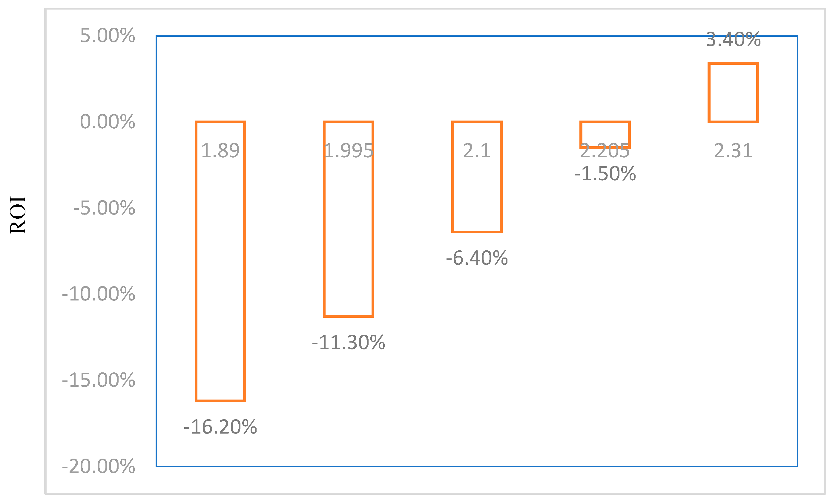
A critical value of C = 211,033 is identified as a strategic threshold. If the government’s cap is below this value, the buyer will opt for Strategy I, while the vendor will choose Strategy II. Conversely, if the cap exceeds this value, each player will select the opposite strategy. This critical value guides strategic decisions and highlights the importance of incorporating negotiation factors to distribute extra profits based on each player’s contribution. For government policy, this critical value suggests that setting caps below or above this threshold can significantly influence market strategies and outcomes. Another critical value, C = 223,786, is crucial for setting reasonable carbon emission quotas. If the quota is below this value, vendors may be reluctant to invest in green technology. This finding underscores the need for governments to set quotas that encourage sustainable investments.

From the vendor’s perspective, the return on investment in green technology is positive only under specific conditions, such as when C = 231,000. This indicates that vendors may be interested in investing in green technology if the return is positive. The study contributes to understanding strategic decision-making under cap-and-trade regulations, emphasizing the importance of critical values and sensitivity coefficients in guiding investments and pricing strategies. It highlights how changes in setup costs, holding costs, and sensitivity coefficients can impact production cycles and inventory management. From the sensitivity analysis, it is shown that:

• If the buyer (retailer) is willing to share more profits, the seller (supplier) can offer higher price discounts to encourage the buyer to place larger orders; this will increase the profits of both parties.
• The critical point of C (the cap of carbon emission) can be a metric for selecting Strategy I and Strategy II. In addition, C is also a key factor affecting ROI. If the value of C is too low, the ROI will be negative, and the company will suffer losses.
• In addition, when the subsidy for carbon emission reduction obtained by the supplier is lower than the critical value, the supplier will suffer cost losses and may be unwilling to invest in green technology. Therefore, the government should set a carbon emission cap above the critical point.
• Extending the production cycle can reduce the setup cost per unit time.
• Reducing the time interval between replenishments can reduce holding costs.
• A higher C_p value (Unit price per carbon emission) can promote lower carbon emission.

For future research, exploring how different regulatory frameworks and technological advancements can further influence these strategies would be beneficial. Additionally, examining the impact of consumer preferences and benefits could provide valuable insights into how businesses can align their strategies with growing eco-consumer demands.

References

1. Daryanto, Y.; Wee, H.M.; Widyadana, G. Low carbon supply chain coordination for imperfect quality deteriorating items. Mathematics 2019, 7, 234. [Google Scholar] [CrossRef]
2. Hua, G.; Cheng, T.C.E.; Wang, S. Managing carbon footprints in inventory management. Int. J. Prod. Econ. 2011, 132, 178–185. [Google Scholar] [CrossRef]
3. Dwicahyani, A.R.; Jauhari, W.A.; Rosyidi, C.N.; Laksono, P.W. Inventory decisions in a two-echelon system with remanufacturing, carbon emission, and energy effects. Cogent Eng. 2017, 4, 1379628. [Google Scholar] [CrossRef]
4. Ghosh, A.; Jha, J.K.; Sarmah, S.P. Optimal lot-sizing under strict carbon cap policy considering stochastic demand. Appl. Math. Model. 2017, 44, 688–704. [Google Scholar] [CrossRef]
5. Tiwari, S.; Daryanto, Y.; Wee, H.M. Sustainable inventory management with deteriorating and imperfect quality items considering carbon emission. J. Clean. Prod. 2018, 192, 281–292. [Google Scholar] [CrossRef]
6. Yang, H.; Chen, W. Retailer-driven carbon emission abatement with consumer environmental awareness and carbon tax: Revenue-sharing versus cost-sharing. Omega 2018, 78, 179–191. [Google Scholar] [CrossRef]
7. Bai, Q.; Xu, J.; Zhang, Y. Emission reduction decision and coordination of a make-to-order supply chain with two products under cap-and-trade regulation. Comput. Ind. Eng. 2018, 119, 131–145. [Google Scholar] [CrossRef]
8. Turki, S.; Sauvey, C.; Rezg, N. Modelling and optimization of a manufacturing/ remanufacturing system with storage facility under carbon cap and trade policy. J. Clean. Prod. 2018, 193, 441–458. [Google Scholar] [CrossRef]
9. Chelly, A.; Nouira, I.; Frein, Y.; Hadj-Alouane, A.B. On the consideration of carbon emissions in modelling-based supply chain literature: The state of the art, relevant features and research gaps. Int. J. Prod. Res. 2019, 57, 4977–5004. [Google Scholar] [CrossRef]
10. Yu, J.C.P.; Yang, P.C.; Lai, X.C. Integrated manufacturer-retailer closed-loop inventory system with price-sensitive return and demand rates. J. Ind. Prod. Eng. 2019, 36, 134–145. [Google Scholar] [CrossRef]
11. Taleizadeh, A.A.; Alizadeh-Basban, N.; Taghi Akhavan Niaki, S. A closed-loop supply chain considering carbon reduction, quality improvement effort, and return policy under two remanufacturing scenarios. J. Clean. Prod. 2019, 232, 1230–1250. [Google Scholar] [CrossRef]
12. Nahr, J.G.; Pasandideh, S.H.R.; Niaki, S.T.A. A robust optimization approach for multi-objective, multi-product, multi-period, closed-loop green supply chain network designs under uncertainty and discount. J. Ind. Prod. Eng. 2020, 37, 1–22. [Google Scholar]
13. Entezaminia, A.; Gharbi, A.; Ouhimmou, M. Environmental hedging point policies for collaborative unreliable manufacturing systems with variant emitting level technologies. J. Clean. Prod. 2020, 250, 119539. [Google Scholar] [CrossRef]
14. Taleizadeh, A.A.; Shokr, I.; Joali, F. Optimizing vendor-managed inventory systems with limited storage capacity and partial backordering under stochastic demand. Rairo-Oper. Res. 2020, 54, 179–209. [Google Scholar] [CrossRef]
15. Ramandi, M.D.; Bafruei, M.K. Effects of government’s policy on supply chain coordination with a periodic review inventory system to reduce greenhouse gas emissions. Comput. Ind. Eng. 2020, 148, 106756. [Google Scholar] [CrossRef]
16. Roy, M.D.; Sana, S.S. Production rate and lot-size dependent lead time reduction strategies in a supply chain model with stochastic demand, controllable setup cost and trade-credit financing. Rairo-Oper. Res. 2021, 55, 1469–1485. [Google Scholar]
17. Rout, C.; Paul, A.; Kumar, R.S.; Chakraborty, D.; Goswami, A. Integrated optimization of inventory, replenishment and vehicle routing for a sustainable supply chain under carbon emission regulations. J. Clean. Prod. 2021, 316, 128256. [Google Scholar] [CrossRef]
18. Jiang, S.; Ye, F.; Lin, Q. Managing green innovation investment in a co-competitive supply chain under capital constraint. J. Clean. Prod. 2021, 291, 125254. [Google Scholar] [CrossRef]
19. Hoque, M. An optimal solution policy to an integrated manufacturer-retailers problem with normal distribution of lead times of delivering equal and unequal sized batches. Opsearch 2021, 58, 483–512. [Google Scholar] [CrossRef]
20. Heydari, J.; Govindan, K.; Basiri, Z. Balancing price and green quality in presence of consumer environmental awareness: A green supply chain coordination approach. Int. J. Prod. Res. 2021, 59, 1957–1975. [Google Scholar] [CrossRef]
21. Yu, J.; Lin, Y.; Wang, K. Coordination-based inventory management of two-echelon supply chain with profit sharing”. Int. J. Syst. Sci. 2013, 44, 1587–1601. [Google Scholar] [CrossRef]
22. Sarkar, B.; Bhuniya, S. A sustainable flexible manufacturing–remanufacturing model with improved service and green investment under variable demand. Expert Syst. Appl. 2022, 202, 117154. [Google Scholar] [CrossRef]
23. Sarkar, B.; Guchhait, R. Ramification of information asymmetry on a green supply chain management with the cap-trade, service, and vendor-managed inventory strategies. Electron. Commer. Res. Appl. 2023, 60, 101274. [Google Scholar] [CrossRef]
24. Guchhait, R.; Sarkar, M.; Sarkar, B.; Yang, L.; AlArjani, A.; Mandal, B. Extended material requirement planning (MRP) within a hybrid energy-enabled smart production system. J. Ind. Inf. Integr. 2024, 42, 100717. [Google Scholar] [CrossRef]
25. Guchhait, R.; Sarkar, B. Economic evaluation of an outsourced fourth-party logistics (4PL) under a flexible production system. Int. J. Prod. Econ. 2025, 279, 109440. [Google Scholar]
Figure 1. The flows of a two-echelon supply chain [21].
Mathematics 13 01761 g001
Figure 2. The different scenarios are characterized by the relationship between the vendor and the buyer.
Mathematics 13 01761 g002
Figure 3. Cap C vs. discount price Pb.
Mathematics 13 01761 g003
Figure 4. The relationship between T P v ,   T C v g ,   T P v # , and cap C.
Mathematics 13 01761 g004
Figure 5. Return on investment vs. cap C (105).
Mathematics 13 01761 g005