

A Novel Empirical Interpolation Surrogate for Digital Twin Wave-Based Structural Health Monitoring with MATLAB Implementation


Abstract
1. Introduction
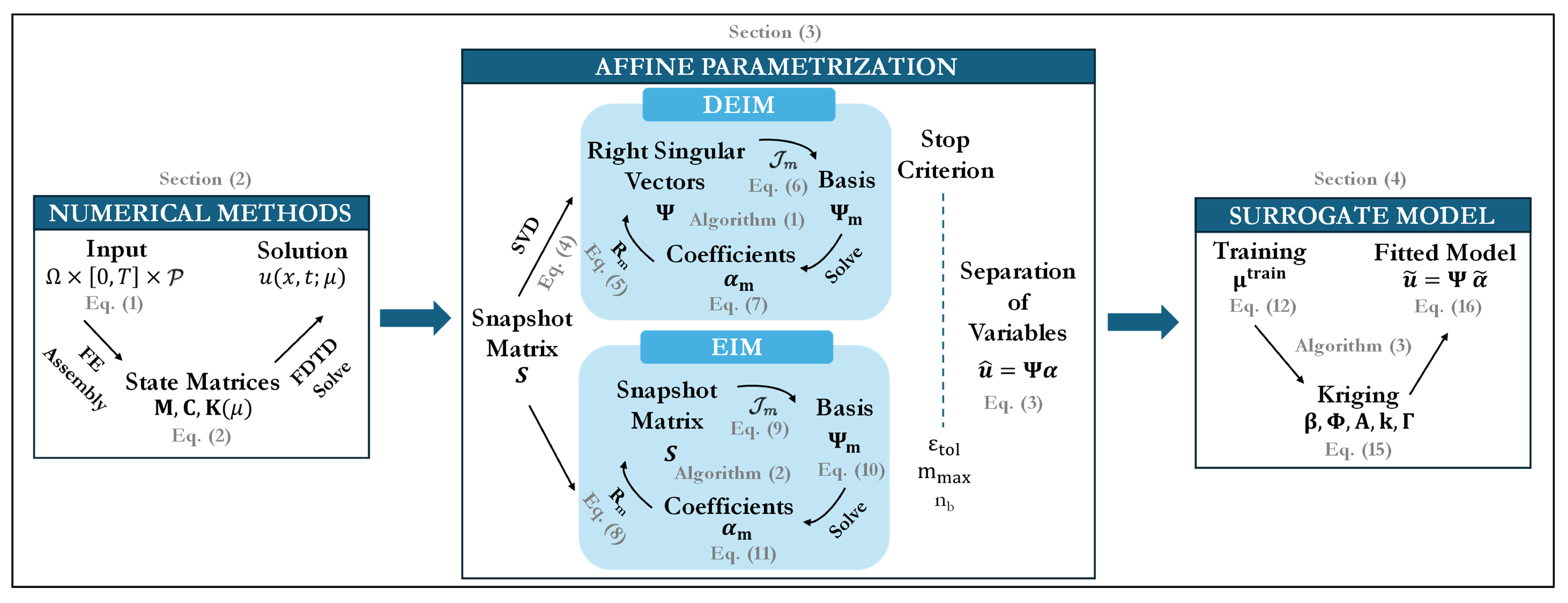
2. Methodology
2.1. Governing Equations
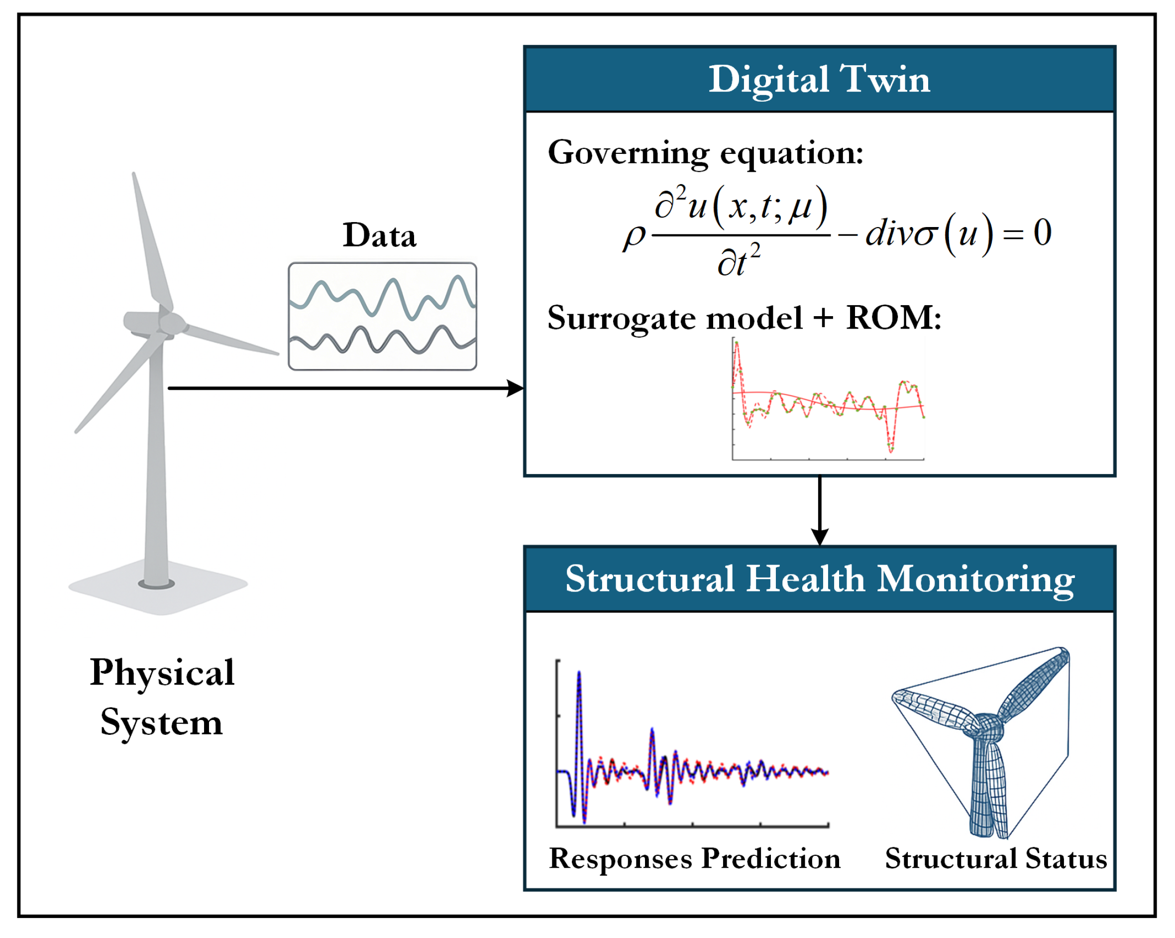
2.2. Affine Parametrization of the Solution
2.2.1. Discrete Empirical Interpolation Method (DEIM)
| Algorithm 1: Discrete Empirical Interpolation (DEIM) |
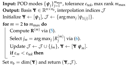 |
2.2.2. Continuous Empirical Interpolation Method (EIM)
| Algorithm 2: Continuous Empirical Interpolation (EIM) |
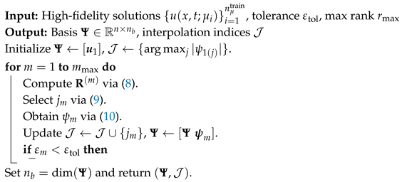 |
2.3. Kriging Surrogate for the Coefficients
| Algorithm 3: Offline–online Kriging surrogate for a coefficient |
Input: Training set ; snapshots ; regression basis Output: Predictor for any query Offline calibration; ; ; for ; Online prediction;
; ; return |
3. Numerical Results and Discussion
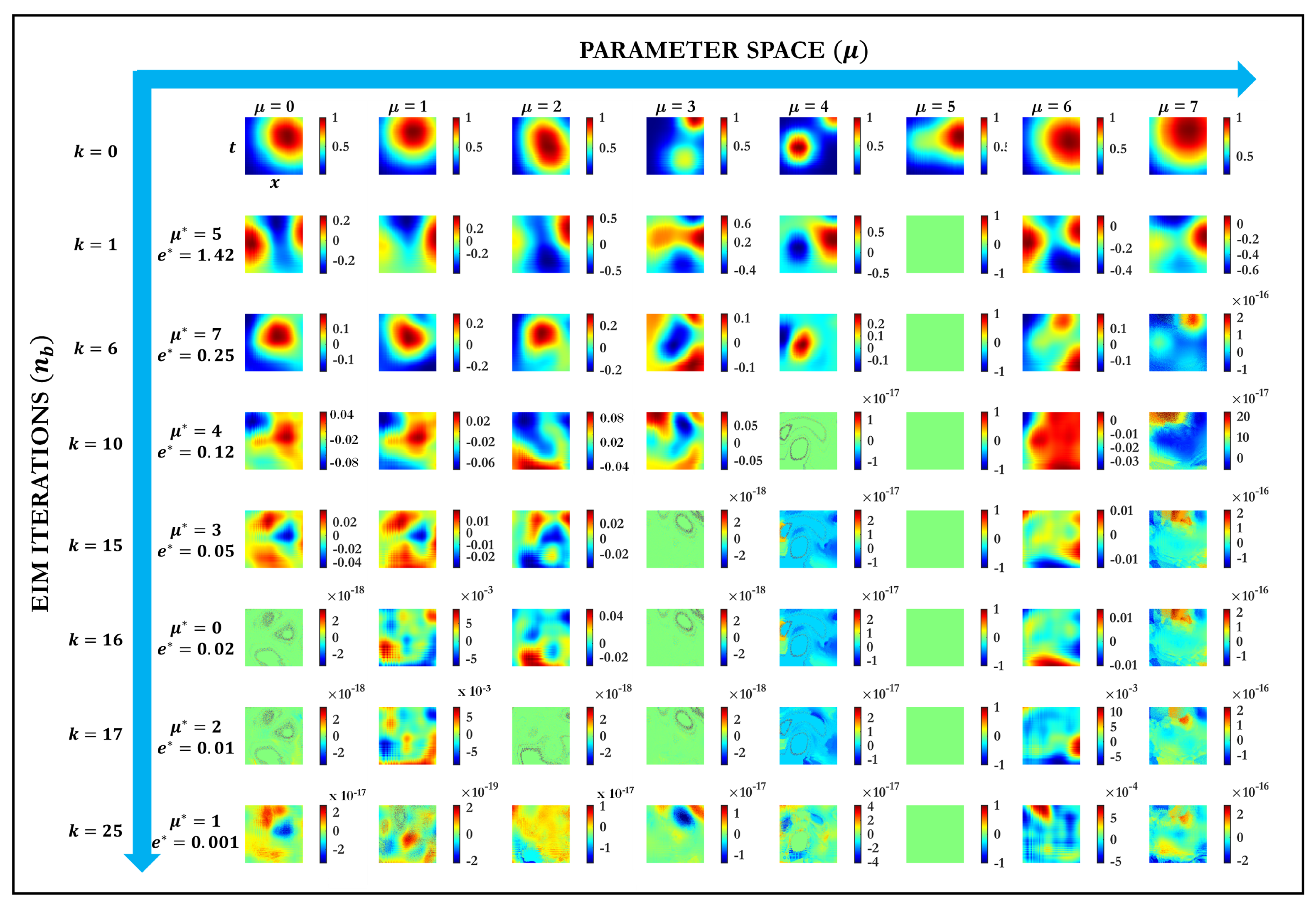
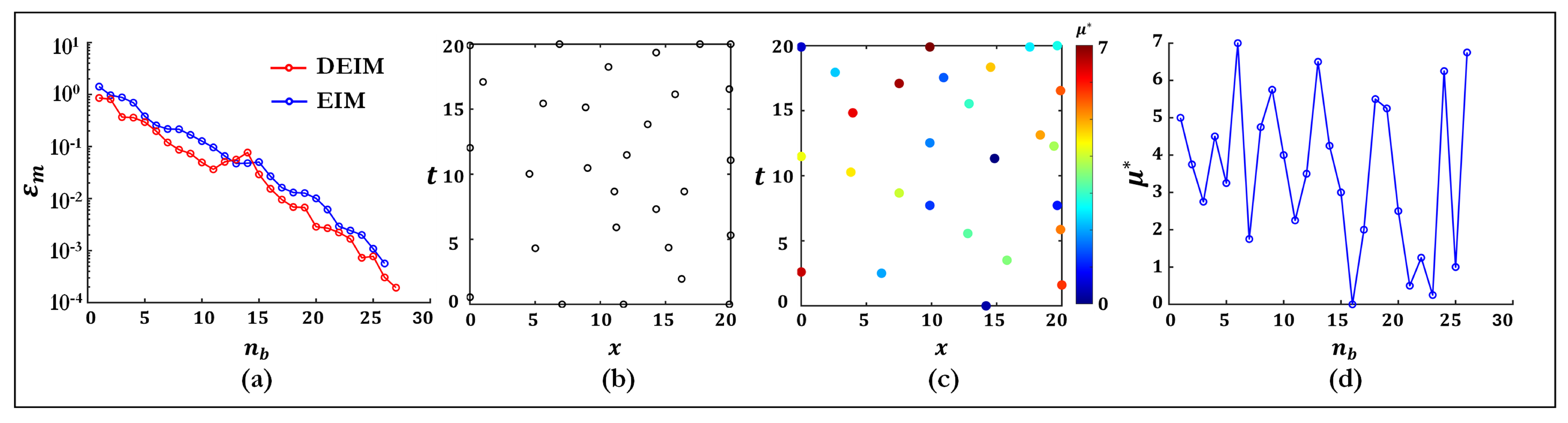
3.1. Analytical Case Study: Convergence on a Parameterized Double-Gaussian Pulse
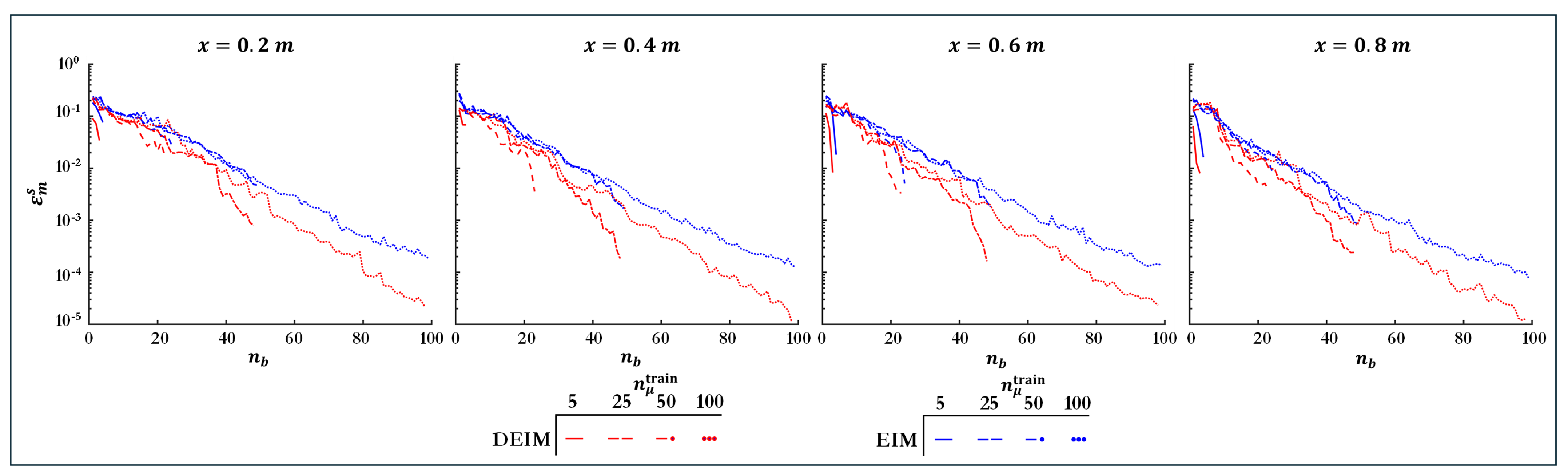
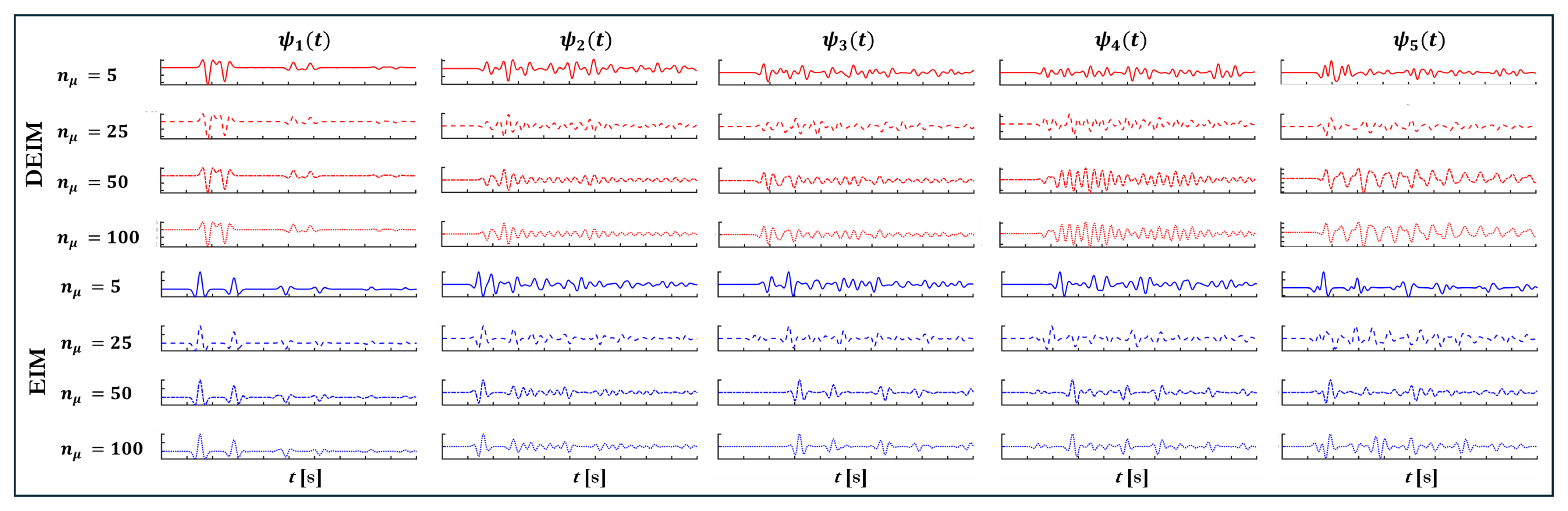
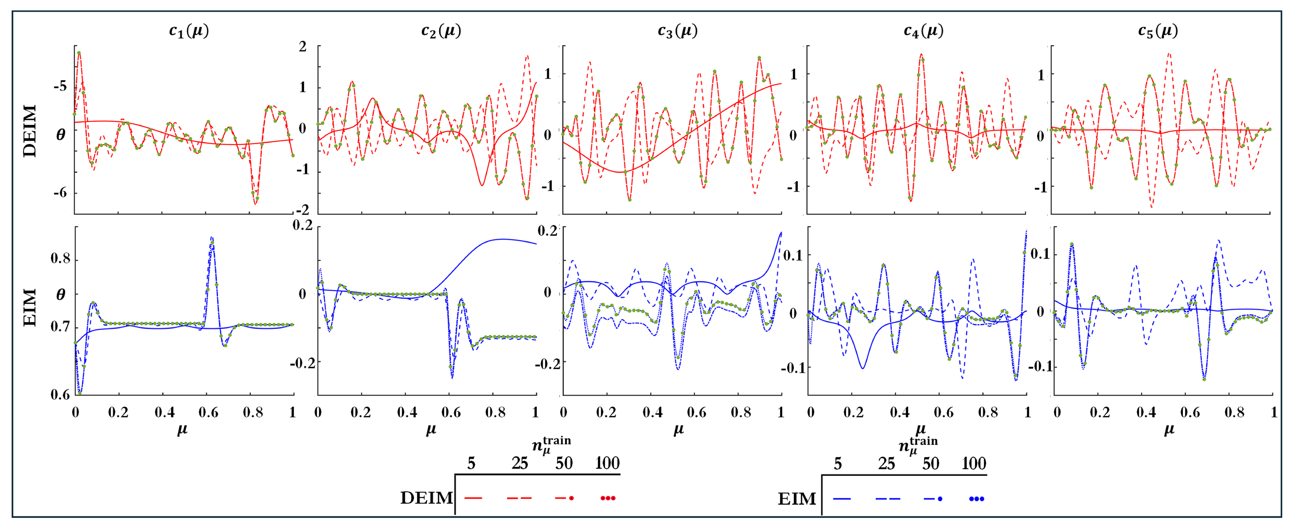
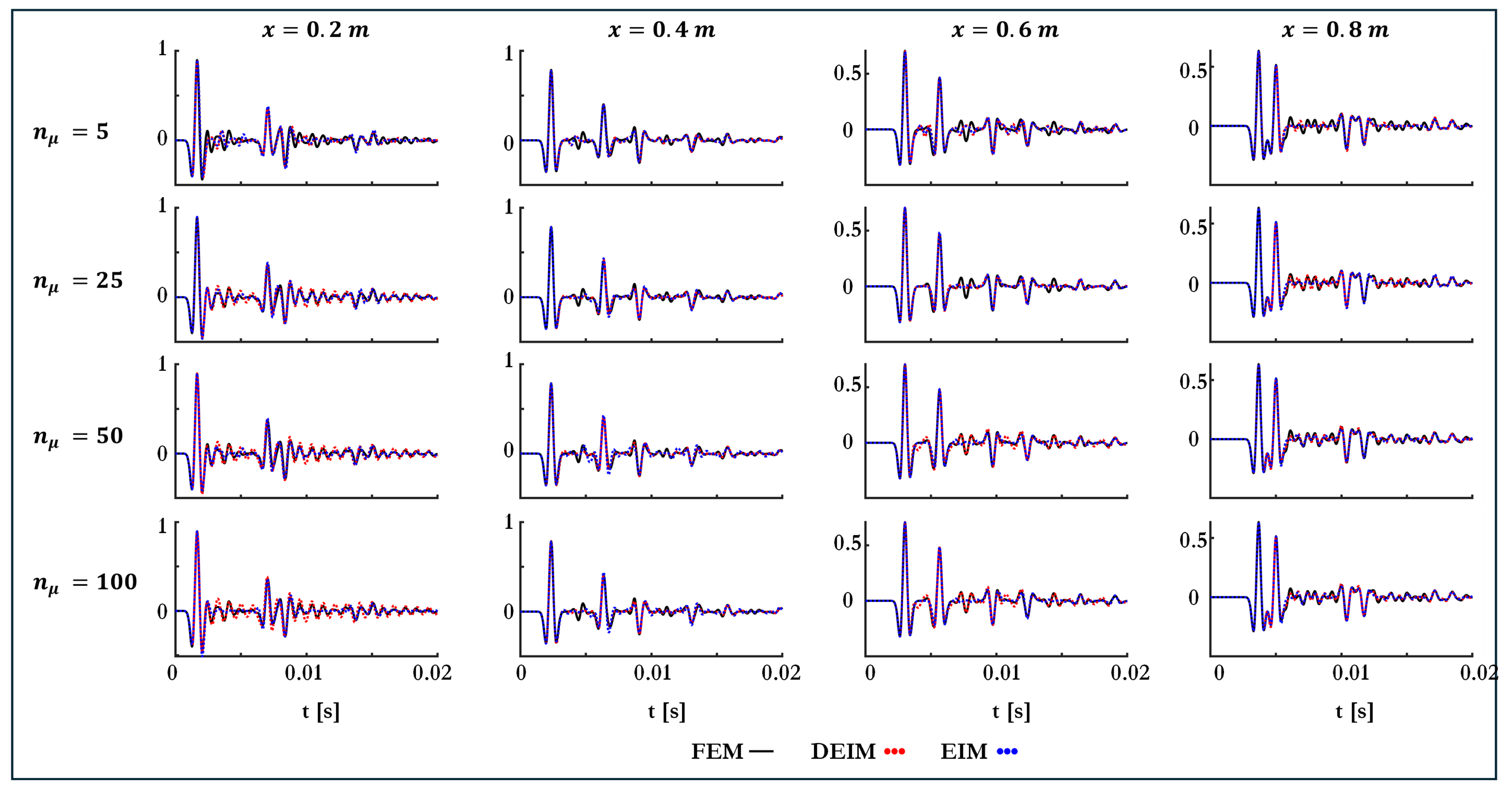
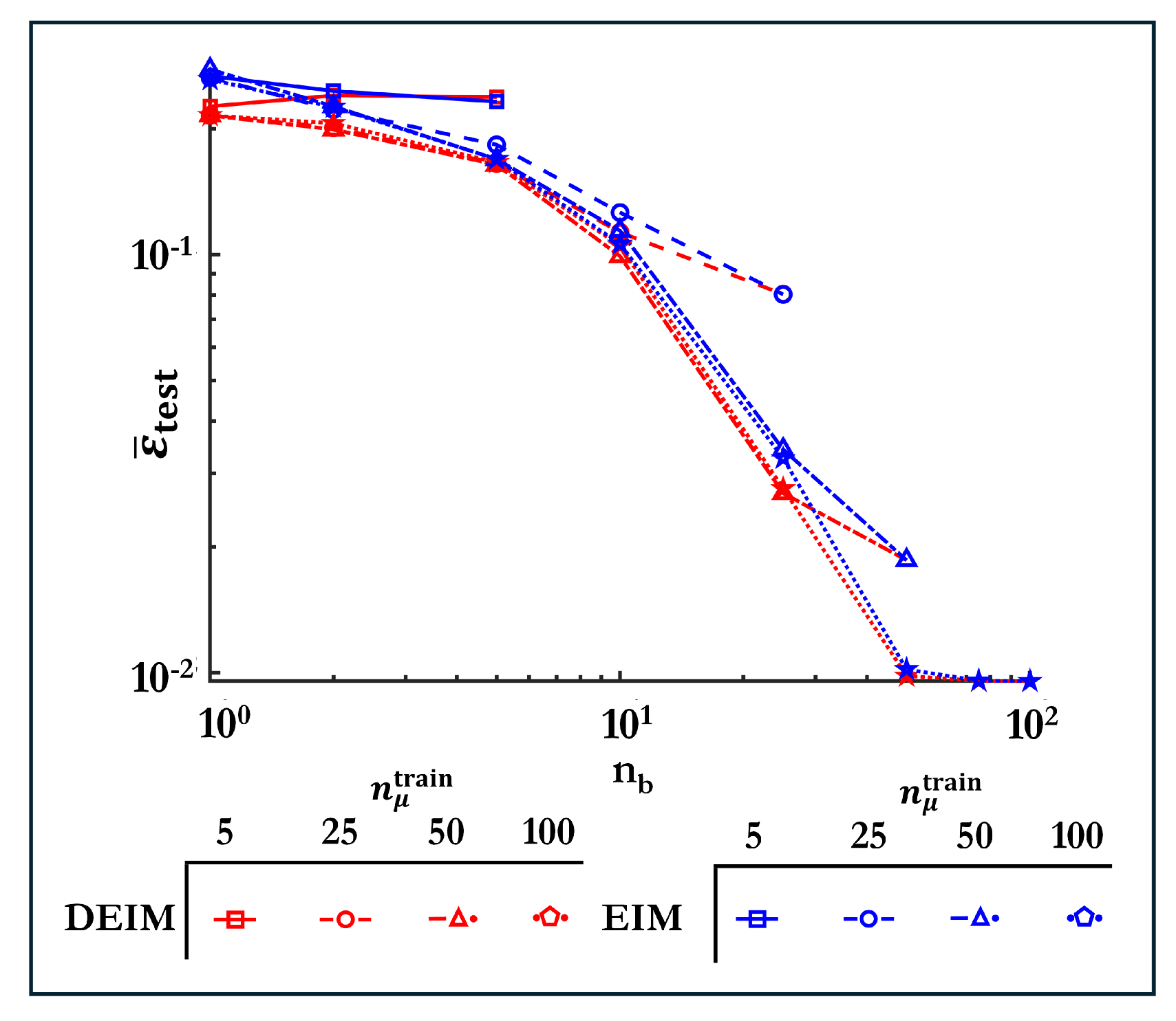
3.2. Guided-Wave Digital Twin for a Prismatic Beam with Localized Stiffness Defect
4. Conclusions and Future Perspectives
Author Contributions
Funding
Data Availability Statement
Acknowledgments
Conflicts of Interest
Appendix A. Parametrized Double-Gaussian Pulse
Appendix B. Nomenclature

| General | Model-Order Reduction | ||
|---|---|---|---|
| Symbol | Meaning | Symbol | Meaning |
| x | Spatial position | Approximated solution | |
| Physical domain | Scalar-valued coefficients | ||
| Real number | Basis functions | ||
| t | Time | Singular values | |
| Damage parameter | Right singular vectors | ||
| Parameter space | Left singular vectors | ||
| u | Displacement | Interpolation indices | |
| Mass density | Residual | ||
| Stress | Boolean matrix | ||
| Strain tensor | Reconstruction error | ||
| ∇ | Gradient operator | Maximum error tolerance | |
| Tensor field | Maximum iteration limit | ||
| Mass | Regression functions | ||
| Rayleigh damping | Regression coefficient vector | ||
| Stiffness matrices | Local bias | ||
| — | — | Correlation function | |
| — | — | Process variance | |
| — | — | Roughness parameter | |
Appendix C. Abbreviations
| Abbreviation | Full Term |
|---|---|
| CFL | Courant–Friedrichs–Lewy condition |
| DEIM | Discrete Empirical Interpolation Method |
| DOF | Degrees of Freedom |
| EIM | Empirical Interpolation Method |
| FCN | Fully Convolutional Network |
| FEM | Finite-Element Method |
| GP | Gaussian Process |
| IIRS | Iterated Improved Reduced System |
| IRS | Improved Reduced System |
| LSTM | Long Short-Term Memory |
| MOR | Model Order Reduction |
| NARX | Nonlinear Autoregressive with Exogenous Input |
| ODE | Ordinary Differential Equation |
| PDE | Partial Differential Equation |
| PCE | Polynomial Chaos Expansion |
| POD | Proper Orthogonal Decomposition |
| ROM | Reduced-Order Model |
| SEREP | System Equivalent Reduction Expansion Process |
| SHM | Structural Health Monitoring |
| SVD | Singular Value Decomposition |
References
- Farrar, C.R.; Worden, K. An introduction to structural health monitoring. Philos. Trans. R. Soc. Math. Phys. Eng. Sci. 2007, 365, 303–315. [Google Scholar] [CrossRef] [PubMed]
- Mardanshahi, A.; Sreekumar, A.; Yang, X.; Barman, S.K.; Chronopoulos, D. Sensing Techniques for Structural Health Monitoring: A State-of-the-Art Review on Performance Criteria and New-Generation Technologies. Sensors 2025, 25, 1424. [Google Scholar] [CrossRef] [PubMed]
- Marwala, T. Finite Element Model Updating Using Computational Intelligence Techniques: Applications to Structural Dynamics; Springer Science & Business Media: Cham, Switzerland, 2010. [Google Scholar]
- Chinesta, F.; Cueto, E.; Abisset-Chavanne, E.; Duval, J.L.; Khaldi, F.E. Virtual, digital and hybrid twins: A new paradigm in data-based engineering and engineered data. Arch. Comput. Methods Eng. 2020, 27, 105–134. [Google Scholar] [CrossRef]
- Fink, O.; Wang, Q.; Svensen, M.; Dersin, P.; Lee, W.J.; Ducoffe, M. Potential, challenges and future directions for deep learning in prognostics and health management applications. Eng. Appl. Artif. Intell. 2020, 92, 103678. [Google Scholar] [CrossRef]
- Torzoni, M.; Manzoni, A.; Mariani, S. Structural health monitoring of civil structures: A diagnostic framework powered by deep metric learning. Comput. Struct. 2022, 271, 106858. [Google Scholar] [CrossRef]
- Avci, O.; Abdeljaber, O.; Kiranyaz, S.; Hussein, M.; Gabbouj, M.; Inman, D.J. A review of vibration-based damage detection in civil structures: From traditional methods to Machine Learning and Deep Learning applications. Mech. Syst. Signal Process. 2021, 147, 107077. [Google Scholar] [CrossRef]
- Entezami, A.; Sarmadi, H.; Behkamal, B.; Mariani, S. Big data analytics and structural health monitoring: A statistical pattern recognition-based approach. Sensors 2020, 20, 2328. [Google Scholar] [CrossRef]
- Kamariotis, A.; Chatzi, E.; Straub, D. Value of information from vibration-based structural health monitoring extracted via Bayesian model updating. Mech. Syst. Signal Process. 2022, 166, 108465. [Google Scholar] [CrossRef]
- Azam, S.E.; Mariani, S. Online damage detection in structural systems via dynamic inverse analysis: A recursive Bayesian approach. Eng. Struct. 2018, 159, 28–45. [Google Scholar] [CrossRef]
- Corigliano, A.; Mariani, S. Parameter identification in explicit structural dynamics: Performance of the extended Kalman filter. Comput. Methods Appl. Mech. Eng. 2004, 193, 3807–3835. [Google Scholar] [CrossRef]
- Azam, S.E.; Chatzi, E.; Papadimitriou, C. A dual Kalman filter approach for state estimation via output-only acceleration measurements. Mech. Syst. Signal Process. 2015, 60, 866–886. [Google Scholar] [CrossRef]
- Mitra, M.; Gopalakrishnan, S. Guided wave based structural health monitoring: A review. Smart Mater. Struct. 2016, 25, 053001. [Google Scholar] [CrossRef]
- Yang, Z.; Yang, H.; Tian, T.; Deng, D.; Hu, M.; Ma, J.; Gao, D.; Zhang, J.; Ma, S.; Yang, L.; et al. A review on guided-ultrasonic-wave-based structural health monitoring: From fundamental theory to machine learning techniques. Ultrasonics 2023, 133, 107014. [Google Scholar] [CrossRef] [PubMed]
- Wierach, P. Lamb-Wave Based Structural Health Monitoring in Polymer Composites; Springer: Cham, Switzerland, 2017. [Google Scholar]
- Taddei, T.; Penn, J.; Yano, M.; Patera, A.T. Simulation-based classification; a model-order-reduction approach for structural health monitoring. Arch. Comput. Methods Eng. 2018, 25, 23–45. [Google Scholar] [CrossRef]
- Rosafalco, L.; Corigliano, A.; Manzoni, A.; Mariani, S. A hybrid structural health monitoring approach based on reduced-order modelling and deep learning. Proceedings 2020, 42, 67. [Google Scholar] [CrossRef]
- Sreekumar, A.; Triantafyllou, S.P.; Chevillotte, F.; Bécot, F.X. Resolving vibro-acoustics in poroelastic media via a multiscale virtual element method. Int. J. Numer. Methods Eng. 2023, 124, 1510–1546. [Google Scholar] [CrossRef]
- Sreekumar, A.; Barman, S.K. Physics-informed model order reduction for laminated composites: A Grassmann manifold approach. Compos. Struct. 2025, 361, 119035. [Google Scholar] [CrossRef]
- Rixen, D.J. A dual Craig–Bampton method for dynamic substructuring. J. Comput. Appl. Math. 2004, 168, 383–391. [Google Scholar] [CrossRef]
- Arasan, U.; Sreekumar, A.; Chevillotte, F.; Triantafyllou, S.; Chronopoulos, D.; Gourdon, E. Condensed finite element scheme for symmetric multi-layer structures including dilatational motion. J. Sound Vib. 2022, 536, 117105. [Google Scholar] [CrossRef]
- Guyan, R.J. Reduction of stiffness and mass matrices. AIAA J. 1965, 3, 380. [Google Scholar] [CrossRef]
- Sreekumar, A. Multiscale Aeroelastic Modelling in Porous Composite Structures. Ph.D. Thesis, University of Nottingham, Nottingham, UK, 2022. [Google Scholar]
- O’Callahan, J.C. System equivalent reduction expansion process. In Proceedings of the 7th International Modal Analysis Conference 1989, Las Vegas, NV, USA, 30 January–2 February 1989. [Google Scholar]
- Gordis, J.H. An analysis of the improved reduced system (IRS) model reduction procedure. In Proceedings of the 10th International Modal Analysis Conference 1992, San Diego, CA, USA, 3–7 February 1992; Volume 1, pp. 471–479. [Google Scholar]
- Friswell, M.; Garvey, S.; Penny, J. Model reduction using dynamic and iterated IRS techniques. J. Sound Vib. 1995, 186, 311–323. [Google Scholar] [CrossRef]
- Sreekumar, A.; Chevillotte, F.; Gourdon, E. Numerical condensation for heterogeneous porous materials and metamaterials. In Proceedings of the 10e Convention de l’Association Européenne d’Acoustique, EAA 2023, Turin, Itlay, 11–15 September 2023. [Google Scholar]
- Besselink, B.; Tabak, U.; Lutowska, A.; Van de Wouw, N.; Nijmeijer, H.; Rixen, D.J.; Hochstenbach, M.; Schilders, W. A comparison of model reduction techniques from structural dynamics, numerical mathematics and systems and control. J. Sound Vib. 2013, 332, 4403–4422. [Google Scholar] [CrossRef]
- Flodén, O.; Persson, K.; Sandberg, G. Reduction methods for the dynamic analysis of substructure models of lightweight building structures. Comput. Struct. 2014, 138, 49–61. [Google Scholar] [CrossRef]
- Bai, Z. Krylov subspace techniques for reduced-order modeling of large-scale dynamical systems. Appl. Numer. Math. 2002, 43, 9–44. [Google Scholar] [CrossRef]
- Rosafalco, L.; Torzoni, M.; Manzoni, A.; Mariani, S.; Corigliano, A. Online structural health monitoring by model order reduction and deep learning algorithms. Comput. Struct. 2021, 255, 106604. [Google Scholar] [CrossRef]
- Torzoni, M.; Rosafalco, L.; Manzoni, A. A combined model-order reduction and deep learning approach for structural health monitoring under varying operational and environmental conditions. Eng. Proc. 2020, 2, 94. [Google Scholar]
- Sepehry, N.; Shamshirsaz, M.; Bakhtiari Nejad, F. Low-cost simulation using model order reduction in structural health monitoring: Application of balanced proper orthogonal decomposition. Struct. Control. Health Monit. 2017, 24, e1994. [Google Scholar] [CrossRef]
- Torzoni, M.; Manzoni, A.; Mariani, S. A multi-fidelity surrogate model for structural health monitoring exploiting model order reduction and artificial neural networks. Mech. Syst. Signal Process. 2023, 197, 110376. [Google Scholar] [CrossRef]
- Du, J.; Zeng, J.; Wang, H.; Ding, H.; Wang, H.; Bi, Y. Using acoustic emission technique for structural health monitoring of laminate composite: A novel CNN-LSTM framework. Eng. Fract. Mech. 2024, 309, 110447. [Google Scholar] [CrossRef]
- Luo, H.; Huang, M.; Zhou, Z. A dual-tree complex wavelet enhanced convolutional LSTM neural network for structural health monitoring of automotive suspension. Measurement 2019, 137, 14–27. [Google Scholar] [CrossRef]
- Sengupta, P.; Chakraborty, S. An improved iterative model reduction technique to estimate the unknown responses using limited available responses. Mech. Syst. Signal Process. 2023, 182, 109586. [Google Scholar] [CrossRef]
- Kundu, A.; Adhikari, S. Transient response of structural dynamic systems with parametric uncertainty. J. Eng. Mech. 2014, 140, 315–331. [Google Scholar] [CrossRef]
- Sreekumar, A.; Kougioumtzoglou, I.A.; Triantafyllou, S.P. Filter approximations for random vibroacoustics of rigid porous media. ASCE-ASME J. Risk Uncertain. Eng. Syst. Part B Mech. Eng. 2024, 10, 031201. [Google Scholar] [CrossRef]
- Jacquelin, E.; Baldanzini, N.; Bhattacharyya, B.; Brizard, D.; Pierini, M. Random dynamical system in time domain: A POD-PC model. Mech. Syst. Signal Process. 2019, 133, 106251. [Google Scholar] [CrossRef]
- Gerritsma, M.; Van der Steen, J.B.; Vos, P.; Karniadakis, G. Time-dependent generalized polynomial chaos. J. Comput. Phys. 2010, 229, 8333–8363. [Google Scholar] [CrossRef]
- Xiu, D.; Karniadakis, G.E. The Wiener–Askey polynomial chaos for stochastic differential equations. SIAM J. Sci. Comput. 2002, 24, 619–644. [Google Scholar] [CrossRef]
- Jacquelin, E.; Adhikari, S.; Sinou, J.J.; Friswell, M.I. Polynomial chaos expansion and steady-state response of a class of random dynamical systems. J. Eng. Mech. 2015, 141, 04014145. [Google Scholar] [CrossRef]
- Le Maître, O.P.; Mathelin, L.; Knio, O.M.; Hussaini, M.Y. Asynchronous time integration for polynomial chaos expansion of uncertain periodic dynamics. Discret. Contin. Dyn. Syst. 2010, 28, 199–226. [Google Scholar] [CrossRef]
- Spiridonakos, M.D.; Chatzi, E.N. Metamodeling of dynamic nonlinear structural systems through polynomial chaos NARX models. Comput. Struct. 2015, 157, 99–113. [Google Scholar] [CrossRef]
- Bhattacharyya, B.; Jacquelin, E.; Brizard, D. Uncertainty quantification of nonlinear stochastic dynamic problem using a Kriging-NARX surrogate model. In Proceedings of the 3rd International Conference on Uncertainty Quantification in Computational Sciences and Engineering, ECCOMAS, Crete, Greece, 24–16 June 2019; pp. 34–46. [Google Scholar]
- Bhattacharyya, B.; Jacquelin, E.; Brizard, D. A Kriging–NARX model for uncertainty quantification of nonlinear stochastic dynamical systems in time domain. J. Eng. Mech. 2020, 146, 04020070. [Google Scholar] [CrossRef]
- Bhattacharyya, B. Uncertainty quantification of dynamical systems by a POD–Kriging surrogate model. J. Comput. Sci. 2022, 60, 101602. [Google Scholar] [CrossRef]
- Zhong, L.; Chen, C.P.; Guo, J.; Zhang, T. Robust incremental broad learning system for data streams of uncertain scale. IEEE Trans. Neural Netw. Learn. Syst. 2024, 36, 7580–7593. [Google Scholar] [CrossRef] [PubMed]
- Samadian, D.; Muhit, I.B.; Dawood, N. Application of data-driven surrogate models in structural engineering: A literature review. Arch. Comput. Methods Eng. 2024, 32, 735–784. [Google Scholar] [CrossRef]
- Hao, P.; Feng, S.; Li, Y.; Wang, B.; Chen, H. Adaptive infill sampling criterion for multi-fidelity gradient-enhanced kriging model. Struct. Multidiscip. Optim. 2020, 62, 353–373. [Google Scholar] [CrossRef]
- Brezzi, F.; Franzone, P.C.; Gianazza, U.; Gilardi, G. Analysis and Numerics of Partial Differential Equations; Springer: Cham, Switzerland, 2013. [Google Scholar]
- Chaturantabut, S.; Sorensen, D.C. Nonlinear model reduction via discrete empirical interpolation. SIAM J. Sci. Comput. 2010, 32, 2737–2764. [Google Scholar] [CrossRef]
- Tiso, P.; Rixen, D.J. Discrete empirical interpolation method for finite element structural dynamics. In Proceedings of the Topics in Nonlinear Dynamics, Volume 1: Proceedings of the 31st IMAC, A Conference on Structural Dynamics, Garden Grove, CA, USA, 11–14 February 2013; Springer: New York, NY, USA, 2013; pp. 203–212. [Google Scholar]
- Nguyen, N.C.; Patera, A.T.; Peraire, J. A ‘best points’ interpolation method for efficient approximation of parametrized functions. Int. J. Numer. Methods Eng. 2008, 73, 521–543. [Google Scholar] [CrossRef]
- Li, Z.; Shan, J.; Gabbert, U. Development of reduced Preisach model using discrete empirical interpolation method. IEEE Trans. Ind. Electron. 2018, 65, 8072–8079. [Google Scholar] [CrossRef]
- Barrault, M.; Maday, Y.; Nguyen, N.C.; Patera, A.T. An ‘empirical interpolation’ method: Application to efficient reduced-basis discretization of partial differential equations. Comptes Rendus Math. 2004, 339, 667–672. [Google Scholar] [CrossRef]
- Dasgupta, A.; Pecht, M. Material failure mechanisms and damage models. IEEE Trans. Reliab. 1991, 40, 531–536. [Google Scholar] [CrossRef]
- Arefi, A.; van der Meer, F.P.; Forouzan, M.R.; Silani, M.; Salimi, M. Micromechanical evaluation of failure models for unidirectional fiber-reinforced composites. J. Compos. Mater. 2020, 54, 791–800. [Google Scholar] [CrossRef]
- Rossi, D.F.; Ferreira, W.G.; Mansur, W.J.; Calenzani, A.F.G. A review of automatic time-stepping strategies on numerical time integration for structural dynamics analysis. Eng. Struct. 2014, 80, 118–136. [Google Scholar] [CrossRef]
- Bhattacharya, K.; Hosseini, B.; Kovachki, N.B.; Stuart, A.M. Model reduction and neural networks for parametric PDEs. SMAI J. Comput. Math. 2021, 7, 121–157. [Google Scholar] [CrossRef]
- Lassila, T.; Rozza, G. Parametric free-form shape design with PDE models and reduced basis method. Comput. Methods Appl. Mech. Eng. 2010, 199, 1583–1592. [Google Scholar] [CrossRef]
- Arefi, A.; Sreekumar, A.; Chronopoulos, D. A Programmable Hybrid Energy Harvester: Leveraging Buckling and Magnetic Multistability. Micromachines 2025, 16, 359. [Google Scholar] [CrossRef]
- Falini, A. A review on the selection criteria for the truncated SVD in Data Science applications. J. Comput. Math. Data Sci. 2022, 5, 100064. [Google Scholar] [CrossRef]
- Van Beers, W.C.; Kleijnen, J.P. Kriging interpolation in simulation: A survey. In Proceedings of the 2004 Winter Simulation Conference, Washington, DC, USA, 5–8 December 2004; IEEE: Piscataway, NJ, USA, 2004; Volume 1. [Google Scholar]
- Sreekumar, A. Wave-Based SHM Empirical Interpolation MATLAB Code. GitHub Repository. Available online: https://github.com/abhimuscat/wave-based-shm-empirical-interpolation-matlab.git (accessed on 25 April 2025).
- Stoter, S. 10–Model Order Reduction–(Discrete) Empirical Interpolation Method (DEIM). YouTube Video. 2023. Available online: https://www.youtube.com/watch?v=L70nwaBAjlQ (accessed on 24 April 2025).
- Gorissen, D.; Couckuyt, I.; Demeester, P.; Dhaene, T.; Crombecq, K. A surrogate modeling and adaptive sampling toolbox for computer based design. J. Mach. Learn. Res. Camb. Mass. 2010, 11, 2051–2055. [Google Scholar]
- Gorissen, D.; Couckuyt, S.; Demeester, Y.; Dhaene, J.; Riche, R.J.L. ooDACE Toolbox; Dual-Licensed Under GNU Affero GPL v3 and Commercial License; iMinds-SUMO Lab, Ghent University: Gent, Belgium, 2009. [Google Scholar]


| Structural | Method | ||||
|---|---|---|---|---|---|
| Parameter | Value | Description | Parameter | Value | Description |
| E | 702 GPa | Young’s modulus | 1 kHz | Central excitation frequency | |
| 7800 kg/m3 | Density | T | 20 ms | Total simulation time | |
| Ns/m | Damping coefficient | 2666 | Number of time-steps | ||
| L | 1.0 m | Beam length | 401 | Physical DOFs | |
| 0.02 m | Damage width | 5, 25, 50, 100 | Training parameters | ||
| D | 0.5 | Material degradation | 250 | Test parameters | |
| 0.2, 0.4, 0.6, 0.8 m | Measurement locations | — | — | — | |
Disclaimer/Publisher’s Note: The statements, opinions and data contained in all publications are solely those of the individual author(s) and contributor(s) and not of MDPI and/or the editor(s). MDPI and/or the editor(s) disclaim responsibility for any injury to people or property resulting from any ideas, methods, instructions or products referred to in the content. |
© 2025 by the authors. Licensee MDPI, Basel, Switzerland. This article is an open access article distributed under the terms and conditions of the Creative Commons Attribution (CC BY) license (https://creativecommons.org/licenses/by/4.0/).
Share and Cite
Sreekumar, A.; Zhong, L.; Chronopoulos, D. A Novel Empirical Interpolation Surrogate for Digital Twin Wave-Based Structural Health Monitoring with MATLAB Implementation. Mathematics 2025, 13, 1730. https://doi.org/10.3390/math13111730
Sreekumar A, Zhong L, Chronopoulos D. A Novel Empirical Interpolation Surrogate for Digital Twin Wave-Based Structural Health Monitoring with MATLAB Implementation. Mathematics. 2025; 13(11):1730. https://doi.org/10.3390/math13111730
Chicago/Turabian StyleSreekumar, Abhilash, Linjun Zhong, and Dimitrios Chronopoulos. 2025. "A Novel Empirical Interpolation Surrogate for Digital Twin Wave-Based Structural Health Monitoring with MATLAB Implementation" Mathematics 13, no. 11: 1730. https://doi.org/10.3390/math13111730
APA StyleSreekumar, A., Zhong, L., & Chronopoulos, D. (2025). A Novel Empirical Interpolation Surrogate for Digital Twin Wave-Based Structural Health Monitoring with MATLAB Implementation. Mathematics, 13(11), 1730. https://doi.org/10.3390/math13111730