Figure 1.
Latin Hypercube Sampling: Interval boxes and their corresponding midpoints. In (a) two- and (b) three-dimensional space.
Figure 1.
Latin Hypercube Sampling: Interval boxes and their corresponding midpoints. In (a) two- and (b) three-dimensional space.
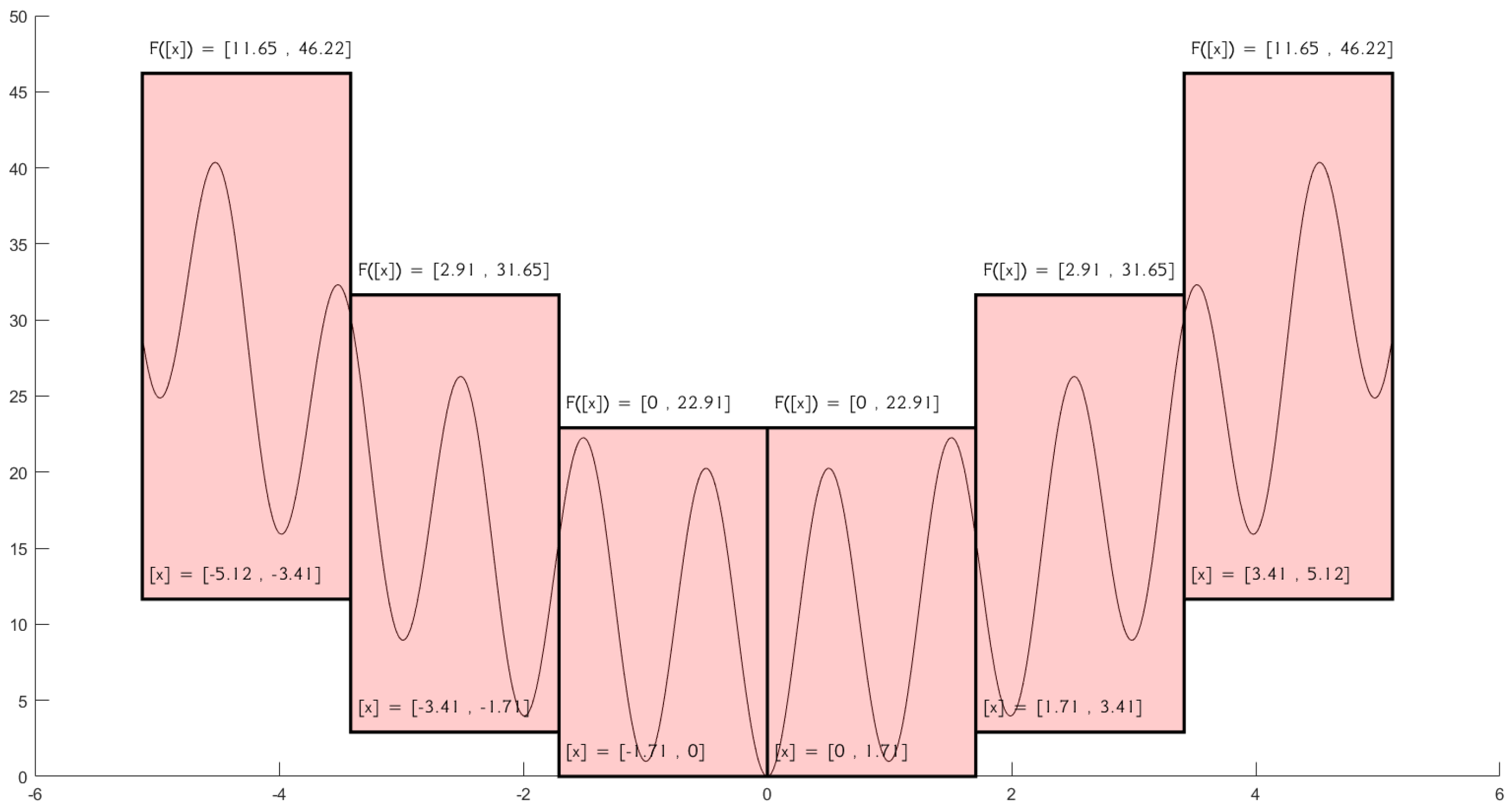
Figure 2.
One−dimensional Rastrigin function: Range overestimation on six-box partition. The two middle boxes are identified as the most promising for deeper local search.
Figure 2.
One−dimensional Rastrigin function: Range overestimation on six-box partition. The two middle boxes are identified as the most promising for deeper local search.
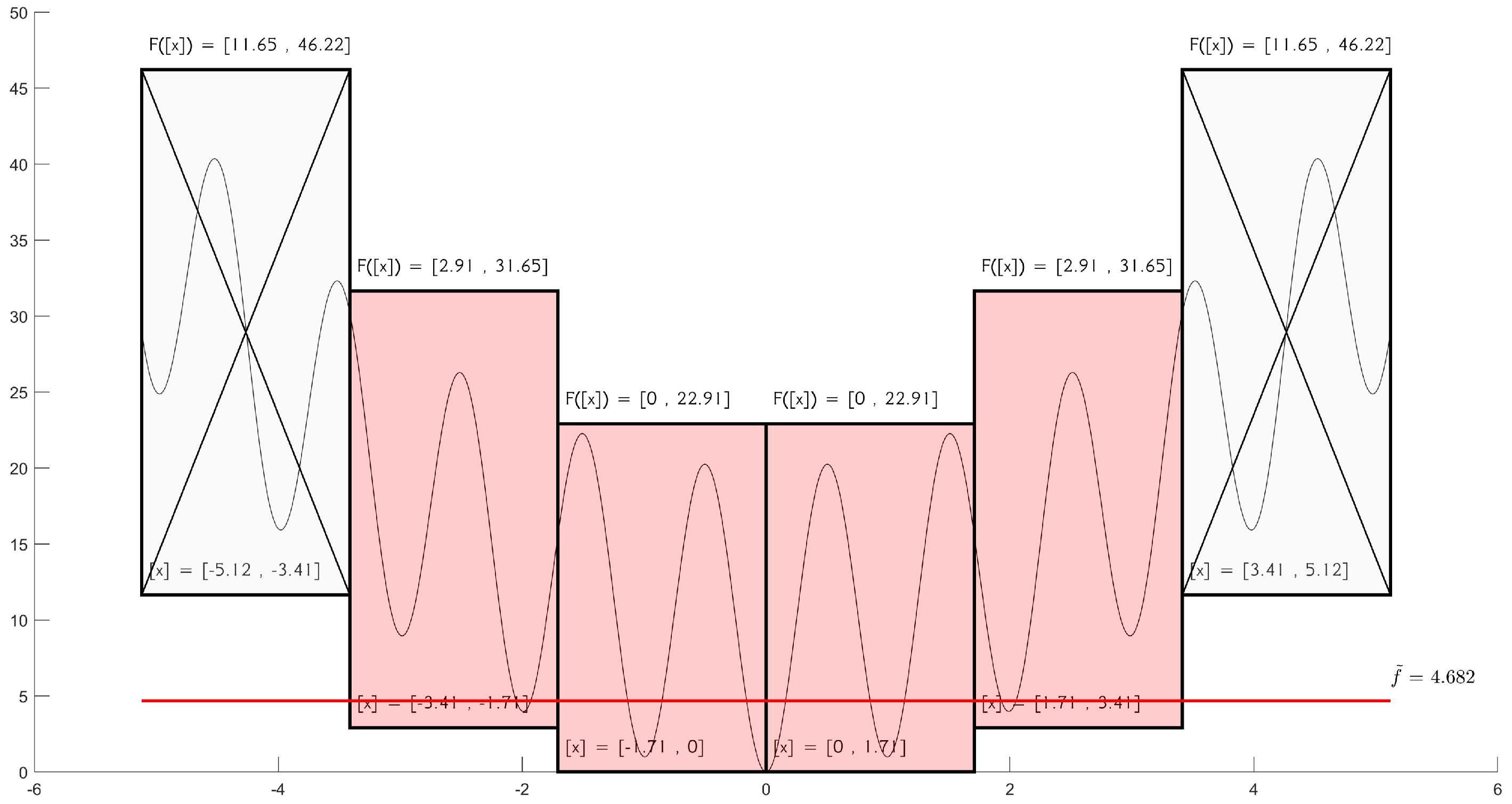
Figure 3.
One−dimensional Rastrigin function: Application of the cut-off test results in the exclusion of 2 out of 6 interval boxes.
Figure 3.
One−dimensional Rastrigin function: Application of the cut-off test results in the exclusion of 2 out of 6 interval boxes.
Figure 4.
Flowchart of the proposed selective multistart optimization framework. The method combines Latin Hypercube Sampling, interval analysis, and local search with termination and pruning criteria.
Figure 4.
Flowchart of the proposed selective multistart optimization framework. The method combines Latin Hypercube Sampling, interval analysis, and local search with termination and pruning criteria.
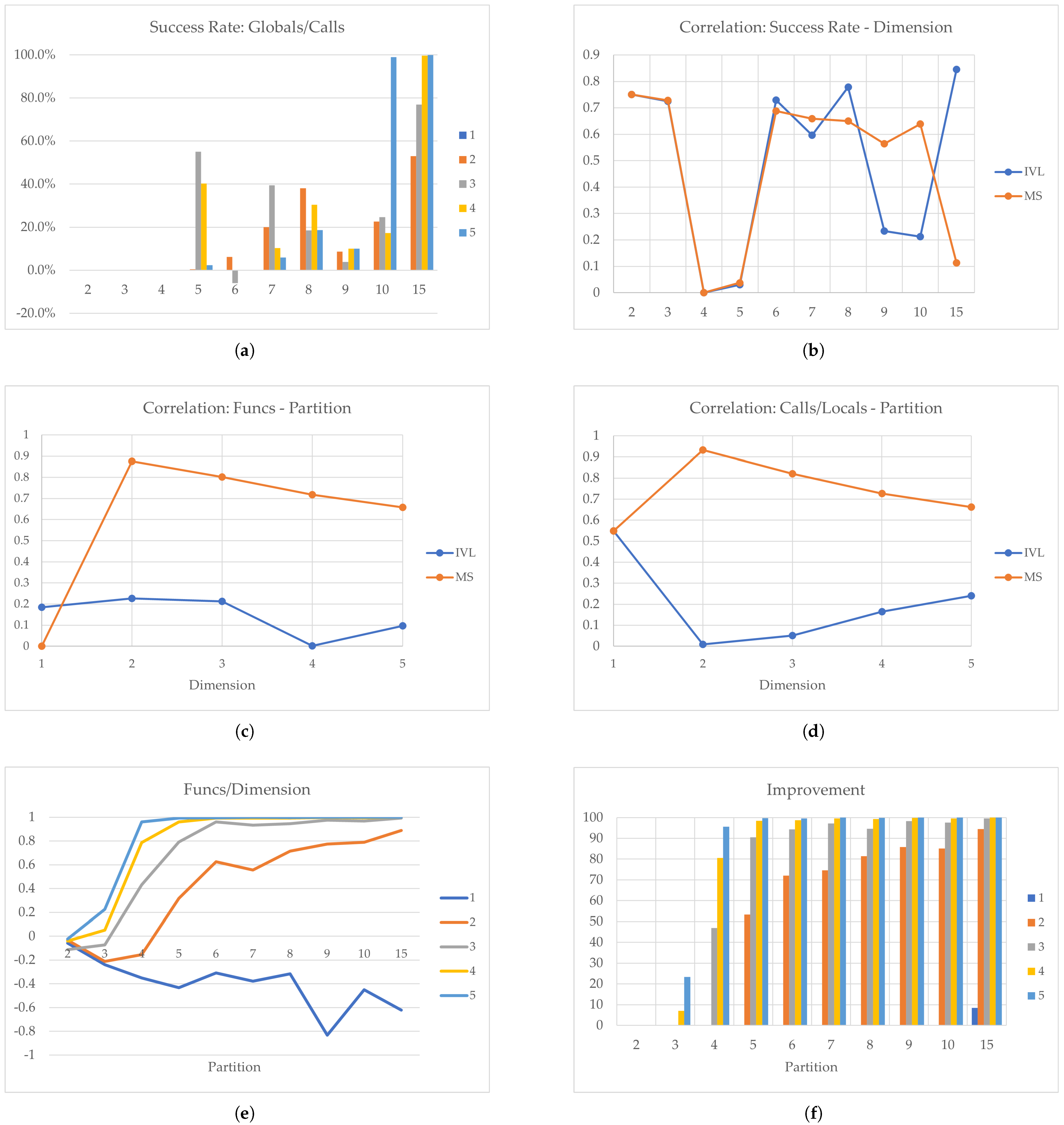
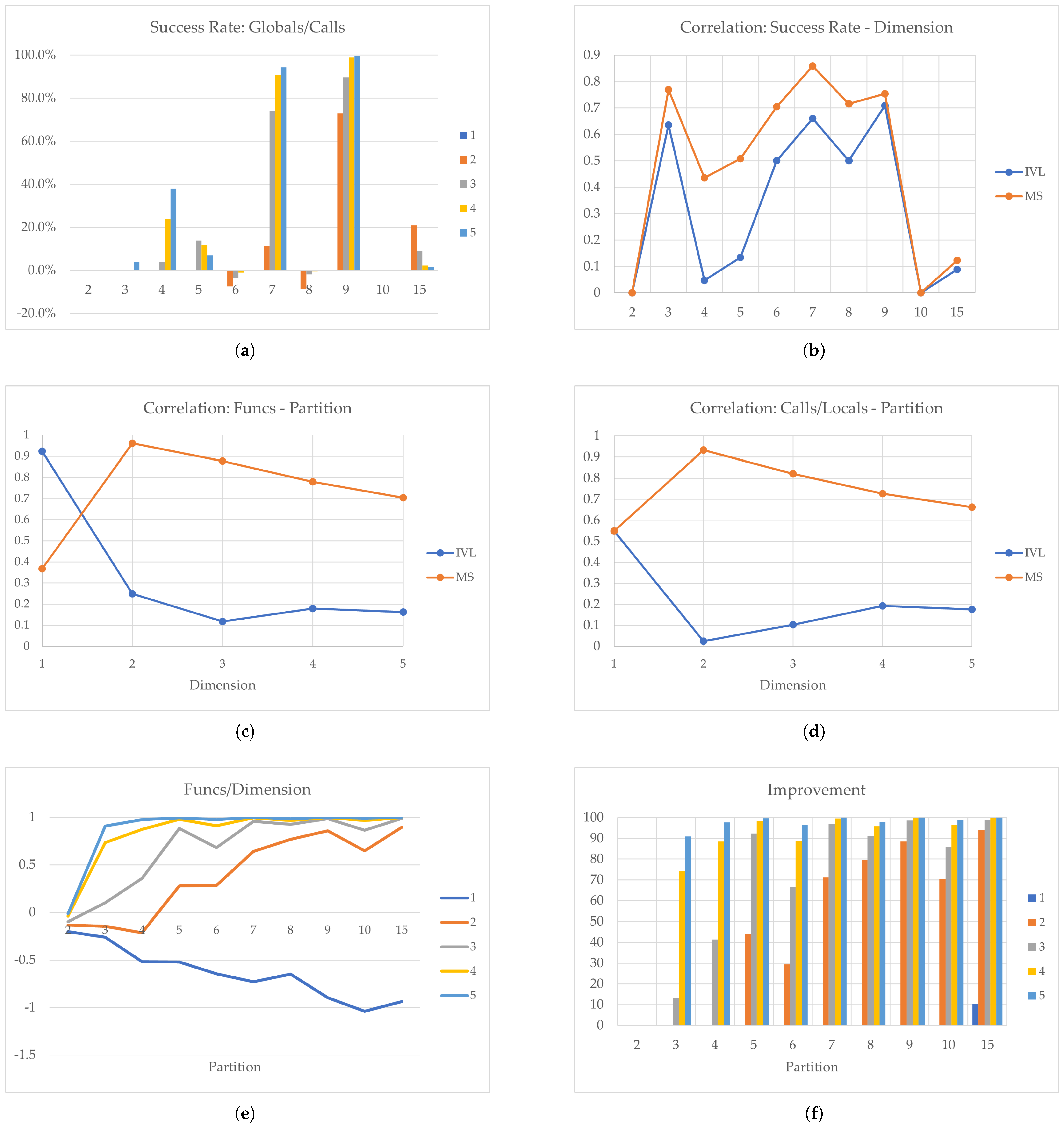
Figure 5.
Ackley Function: (a) Success Rate, (b) Correlation: Success Rate−Partition, (c) Correlation: Function Evaluations−Partition, (d) Correlation: Calls/Locals−Partition, (e) Function Evaluations/Dimension, and (f) Improvement.
Figure 5.
Ackley Function: (a) Success Rate, (b) Correlation: Success Rate−Partition, (c) Correlation: Function Evaluations−Partition, (d) Correlation: Calls/Locals−Partition, (e) Function Evaluations/Dimension, and (f) Improvement.
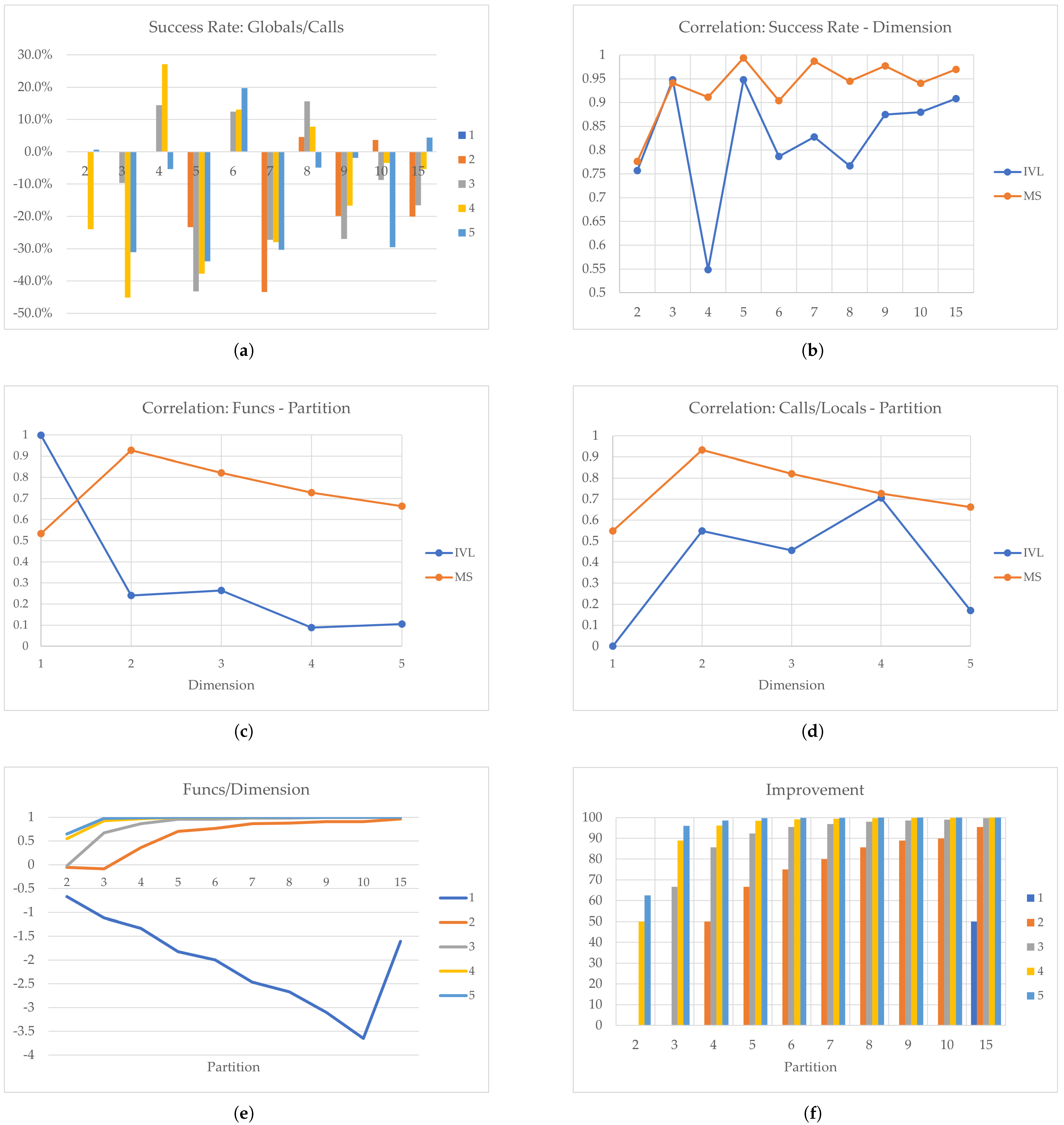
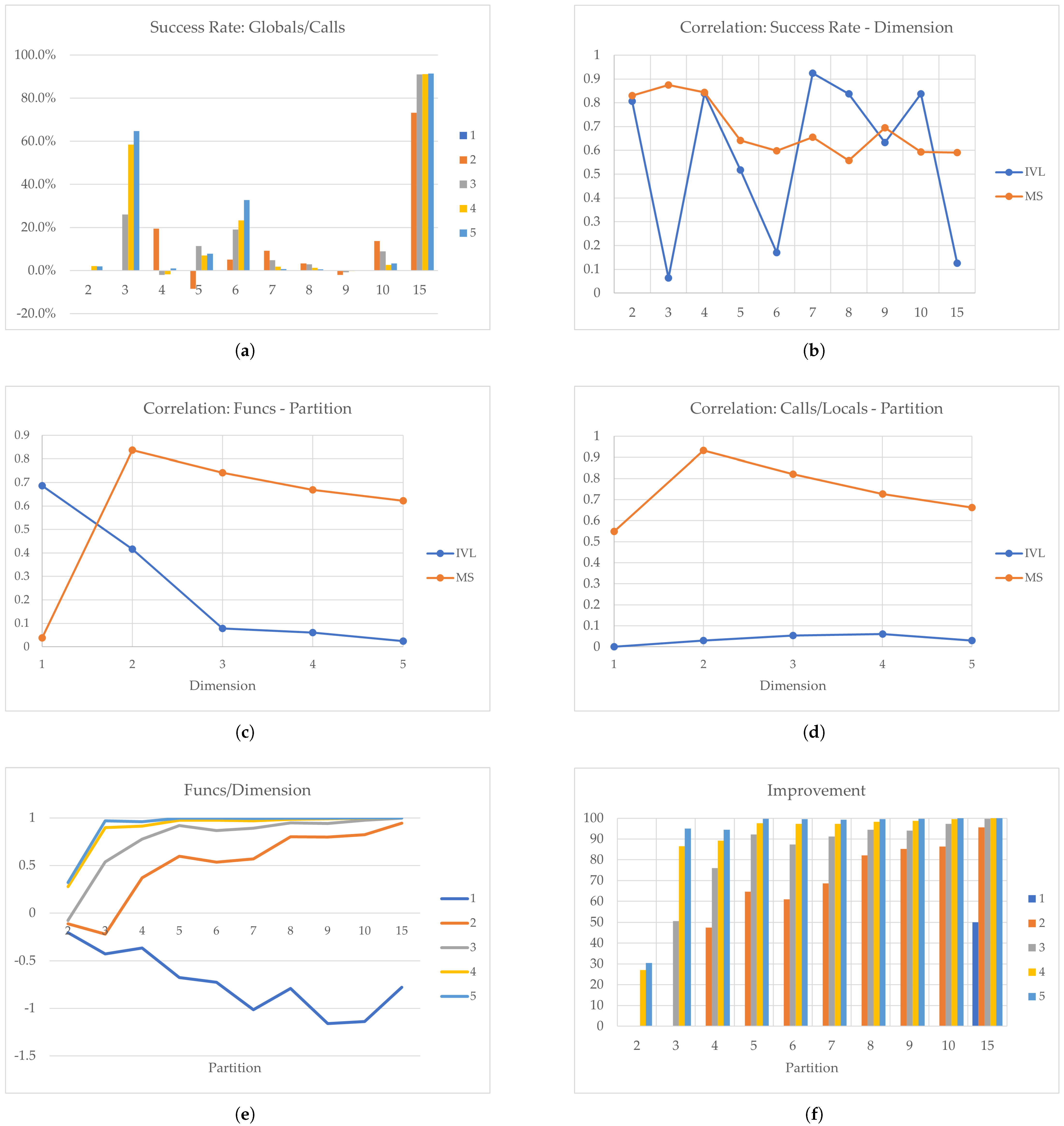
Figure 6.
Dixon–Price Function: (a) Success Rate, (b) Correlation: Success Rate−Partition, (c) Correlation: Function Evaluations−Partition, (d) Correlation: Calls/Locals−Partition, (e) Function Evaluations/Dimension, and (f) Improvement.
Figure 6.
Dixon–Price Function: (a) Success Rate, (b) Correlation: Success Rate−Partition, (c) Correlation: Function Evaluations−Partition, (d) Correlation: Calls/Locals−Partition, (e) Function Evaluations/Dimension, and (f) Improvement.
Figure 7.
Levy Function: (a) Success Rate, (b) Correlation: Success Rate−Partition, (c) Correlation: Function Evaluations−Partition, (d) Correlation: Calls/Locals−Partition, (e) Function Evaluations/Dimension, and (f) Improvement.
Figure 7.
Levy Function: (a) Success Rate, (b) Correlation: Success Rate−Partition, (c) Correlation: Function Evaluations−Partition, (d) Correlation: Calls/Locals−Partition, (e) Function Evaluations/Dimension, and (f) Improvement.
Figure 8.
Rastrigin Function: (a) Success Rate, (b) Correlation: Success Rate−Partition, (c) Correlation: Function Evaluations−Partition, (d) Correlation: Calls/Locals−Partition, (e) Function Evaluations/Dimension, and (f) Improvement.
Figure 8.
Rastrigin Function: (a) Success Rate, (b) Correlation: Success Rate−Partition, (c) Correlation: Function Evaluations−Partition, (d) Correlation: Calls/Locals−Partition, (e) Function Evaluations/Dimension, and (f) Improvement.
Figure 9.
Rosenbrock Function: (a) Success Rate, (b) Correlation: Success Rate−Partition, (c) Correlation: Function Evaluations−Partition, (d) Correlation: Calls/Locals−Partition, (e) Function Evaluations/Dimension, and (f) Improvement.
Figure 9.
Rosenbrock Function: (a) Success Rate, (b) Correlation: Success Rate−Partition, (c) Correlation: Function Evaluations−Partition, (d) Correlation: Calls/Locals−Partition, (e) Function Evaluations/Dimension, and (f) Improvement.
Table 1.
Performance metrics of the Ackley function: success rate, coefficient of variation, and efficiency with respect to dimension and partition size. Entries marked with an asterisk (*) correspond to cases of division by zero.
Table 1.
Performance metrics of the Ackley function: success rate, coefficient of variation, and efficiency with respect to dimension and partition size. Entries marked with an asterisk (*) correspond to cases of division by zero.
| | 2 | 3 | 4 | 5 | 6 | 7 | 8 | 9 | 10 | 15 |
|---|
| | SR | CV | Eff | SR | CV | Eff | SR | CV | Eff | SR | CV | Eff | SR | CV | Eff | SR | CV | Eff | SR | CV | Eff | SR | CV | Eff | SR | CV | Eff | SR | CV | Eff |
| 1 | 0.0% | 0.3028 | 0 | 0.0% | 0.2569 | 0 | * | −0.1525 | * | 0.0% | 0.1509 | 0 | 0.0% | 0.3671 | 0 | 0.0% | 0.1955 | 0 | 0.0% | 0.3364 | 0 | 0.0% | −0.0676 | 0 | 0.0% | 0.3215 | 0 | * | −0.9974 | * |
| 2 | 0.0% | 0.4716 | 0 | 0.0% | −0.2140 | 0 | * | −0.9871 | * | 114.3% | −0.2719 | 3.5918 | 84.7% | −0.5469 | 5.5975 | 293.7% | −0.0925 | 14.5000 | 364.7% | −0.0292 | 24.0223 | 603.1% | −0.2949 | 48.4385 | 272.0% | 0.0554 | 23.9636 | 944.7% | 0.1587 | 186.7186 |
| 3 | * | −1 | * | * | −0.9630 | * | * | −0.2063 | * | 287.4% | −0.6798 | 39.6099 | −100.0% | −0.4055 | −1 | 523.1% | −0.8216 | 217.0871 | 604.9% | 1.1320 | 128.5289 | 5603.1% | −0.0313 | 3251.5635 | 2831.7% | 2.0992 | 1185.9362 | 3013.2% | −0.4369 | 8992.6054 |
| 4 | * | −1 | * | 7.7% | −0.2622 | 0.1590 | * | 0.7140 | * | 413.0% | −0.7551 | 322.2085 | * | −0.9812 | * | 585.3% | −0.7877 | 1650.5924 | 4012.6% | 0.9691 | 5957.2102 | 65,600.0% | −0.0374 | 431,648 | 3948.1% | 3.2576 | 9568.8784 | 32,670.2% | −0.9999 | 1,659,155.57 |
| 5 | * | −1 | * | 30.4% | 1.7762 | 0.7007 | * | 0.5619 | * | 61.5% | −0.8351 | 504.4291 | −100.0% | −0.3149 | −1 | 9069.1% | −0.6731 | 154,131.4182 | 9733.9% | 1.1376 | 64,709.0008 | 56,678.8% | 0.1408 | 3,352,789.865 | 310,244.8% | −0.6970 | 31,034,481.76 | 128,739.5% | −0.9999 | 97,838,136.84 |
Table 2.
Preprocessing times (IVL) for the Ackley function.
Table 2.
Preprocessing times (IVL) for the Ackley function.
| # | 2 | 3 | 4 | 5 | 6 | 7 | 8 | 9 | 10 | 15 |
|---|
| 1 | 0.0010 | 0.0010 | 0.0010 | 0.0010 | 0.0009 | 0.0011 | 0.0013 | 0.0010 | 0.0011 | 0.0019 |
| 2 | 0.0013 | 0.0013 | 0.0025 | 0.0036 | 0.0047 | 0.0097 | 0.0081 | 0.0103 | 0.0114 | 0.0255 |
| 3 | 0.0017 | 0.0046 | 0.0105 | 0.0190 | 0.0309 | 0.0479 | 0.0698 | 0.0977 | 0.1335 | 0.4370 |
| 4 | 0.0036 | 0.0151 | 0.0418 | 0.0987 | 0.2027 | 0.3764 | 0.6386 | 1.0331 | 1.5492 | 7.8323 |
| 5 | 0.0083 | 0.0476 | 0.1914 | 0.5750 | 1.4284 | 3.0881 | 6.0089 | 10.8971 | 18.2944 | 139.6668 |
Table 3.
Processing times (left: IVL, right: MS) for the Ackley function.
Table 3.
Processing times (left: IVL, right: MS) for the Ackley function.
| | 2 | 3 | 4 | 5 | 6 | 7 | 8 | 9 | 10 | 15 |
|---|
| | IVL | MS | IVL | MS | IVL | MS | IVL | MS | IVL | MS | IVL | MS | IVL | MS | IVL | MS | IVL | MS | IVL | MS |
| 1 | 0.0028 | 0.0023 | 0.0014 | 0.0012 | 0.0014 | 0.0014 | 0.0015 | 0.0014 | 0.0017 | 0.0032 | 0.0015 | 0.0013 | 0.0016 | 0.0012 | 0.0016 | 0.0007 | 0.0021 | 0.0016 | 0.0042 | 0.0021 |
| 2 | 0.0022 | 0.0028 | 0.0013 | 0.0013 | 0.0022 | 0.0020 | 0.0015 | 0.0025 | 0.0045 | 0.0032 | 0.0033 | 0.0078 | 0.0013 | 0.0055 | 0.0014 | 0.0064 | 0.0022 | 0.0076 | 0.0012 | 0.0174 |
| 3 | 0.0013 | 0.0010 | 0.0029 | 0.0018 | 0.0025 | 0.0054 | 0.0015 | 0.0102 | 0.0015 | 0.0202 | 0.0015 | 0.0233 | 0.0017 | 0.0414 | 0.0013 | 0.0514 | 0.0075 | 0.0755 | 0.0015 | 0.2476 |
| 4 | 0.0022 | 0.0014 | 0.0066 | 0.0047 | 0.0183 | 0.0190 | 0.0014 | 0.0403 | 0.0019 | 0.0997 | 0.0013 | 0.1524 | 0.0111 | 0.3088 | 0.0014 | 0.4829 | 0.0018 | 0.7626 | 0.0018 | 3.8704 |
| 5 | 0.0037 | 0.0023 | 0.0155 | 0.0131 | 0.0012 | 0.0788 | 0.0016 | 0.1937 | 0.0041 | 0.5943 | 0.0016 | 1.0863 | 0.0022 | 2.5584 | 0.0017 | 4.4787 | 0.0020 | 7.9643 | 0.0020 | 60.5127 |
Table 4.
Performance metrics of the Dixon–Price function: success rate, coefficient of variation, and efficiency with respect to dimension and partition size.
Table 4.
Performance metrics of the Dixon–Price function: success rate, coefficient of variation, and efficiency with respect to dimension and partition size.
| | 2 | 3 | 4 | 5 | 6 | 7 | 8 | 9 | 10 | 15 |
|---|
| | SR | CV | Eff | SR | CV | Eff | SR | CV | Eff | SR | CV | Eff | SR | CV | Eff | SR | CV | Eff | SR | CV | Eff | SR | CV | Eff | SR | CV | Eff | SR | CV | Eff |
| 1 | 0.0% | 0.2101 | 0 | 0.0% | 0.4199 | 0 | 0.0% | 0.4399 | 0 | 0.0% | 0.2797 | 0 | 0.0% | 1.3908 | 0 | 0.0% | 0.5682 | 0 | 0.0% | 0.3316 | 0 | 0.0% | 0.7618 | 0 | 0.0% | 0.3039 | 0 | 0.0% | −0.6575 | 1 |
| 2 | 0.0% | 0.2229 | 0 | 0.0% | 0.4751 | 0 | 0.0% | −0.5037 | 1 | −27.0% | 0.8858 | 1.1892 | 0.0% | −0.9343 | 3 | −51.4% | 0.5272 | 1.4289 | 4.8% | −0.9999 | 6.3353 | −23.2% | 0.6331 | 5.9159 | 3.8% | −1 | 9.3842 | −22.0% | 0.6538 | 16.2592 |
| 3 | 0.0% | 0.6118 | 0 | −19.5% | 0.0600 | 1.4161 | 16.9% | −0.9999 | 7.1803 | −59.9% | 0.0388 | 4.2193 | 14.2% | −0.9999 | 24.1298 | −36.6% | 0.1806 | 19.1703 | 18.5% | −0.9999 | 60.6085 | −34.7% | 0.2013 | 44.8684 | −10.3% | 0.1569 | 86.0603 | −20.8% | 0.2352 | 244.6160 |
| 4 | −31.6% | 0.4245 | 0.3684 | −100.0% | −0.9999 | −1 | 39.4% | −0.9999 | 35.2547 | −70.2% | −0.2633 | 17.7438 | 19.2% | −0.2470 | 145.2101 | −49.0% | −0.0306 | 103.9915 | 11.8% | −0.1052 | 435.6865 | −28.3% | 0.0238 | 431.3220 | −5.2% | 0.0082 | 901.5030 | −8.8% | −0.0777 | 3470.5174 |
| 5 | 1.3% | −0.0625 | 1.7022 | −100.0% | −0.9998 | −1 | −12.1% | 0.0108 | 64.1526 | −97.1% | −0.7973 | 7.9559 | 44.5% | −0.1005 | 984.8924 | −82.2% | −0.4400 | 243.7062 | −10.9% | 0.0142 | 2261.8978 | −4.9% | 0.0079 | 4969.5842 | −66.5% | −0.1214 | 1992.7044 | 10.9% | −0.0598 | 55,054.0632 |
Table 5.
Preprocessing times (IVL) for the Dixon–Price function.
Table 5.
Preprocessing times (IVL) for the Dixon–Price function.
| # | 2 | 3 | 4 | 5 | 6 | 7 | 8 | 9 | 10 | 15 |
|---|
| 1 | 0.0042 | 0.0060 | 0.0017 | 0.0007 | 0.0012 | 0.0013 | 0.0006 | 0.0004 | 0.0003 | 0.0027 |
| 2 | 0.0023 | 0.0009 | 0.0029 | 0.0020 | 0.0027 | 0.0032 | 0.0045 | 0.0058 | 0.0064 | 0.0145 |
| 3 | 0.0011 | 0.0031 | 0.0071 | 0.0129 | 0.0213 | 0.0333 | 0.0498 | 0.0698 | 0.0944 | 0.3144 |
| 4 | 0.0029 | 0.0122 | 0.0334 | 0.0778 | 0.1593 | 0.2972 | 0.5046 | 0.7826 | 1.1926 | 5.9960 |
| 5 | 0.0069 | 0.0393 | 0.1585 | 0.4783 | 1.1812 | 2.5473 | 4.9776 | 8.9981 | 15.2041 | 115.7074 |
Table 6.
Processing times (left: IVL, right: MS) for the Dixon–Price function.
Table 6.
Processing times (left: IVL, right: MS) for the Dixon–Price function.
| | 2 | 3 | 4 | 5 | 6 | 7 | 8 | 9 | 10 | 15 |
|---|
| | IVL | MS | IVL | MS | IVL | MS | IVL | MS | IVL | MS | IVL | MS | IVL | MS | IVL | MS | IVL | MS | IVL | MS |
| 1 | 0.4285 | 0.0204 | 0.0227 | 0.0053 | 0.0283 | 0.0023 | 0.0010 | 0.0008 | 0.0022 | 0.0018 | 0.0009 | 0.0007 | 0.0009 | 0.0005 | 0.0015 | 0.0006 | 0.0008 | 0.0005 | 0.0021 | 0.0015 |
| 2 | 0.1637 | 0.0083 | 0.0065 | 0.0024 | 0.0046 | 0.0050 | 0.0051 | 0.0036 | 0.0012 | 0.0037 | 0.0016 | 0.0051 | 0.0012 | 0.0067 | 0.0014 | 0.0081 | 0.0012 | 0.0092 | 0.0033 | 0.0198 |
| 3 | 0.0025 | 0.0021 | 0.0020 | 0.0038 | 0.0013 | 0.0078 | 0.0014 | 0.0147 | 0.0020 | 0.0241 | 0.0015 | 0.0400 | 0.0022 | 0.0567 | 0.0013 | 0.0781 | 0.0014 | 0.1073 | 0.0012 | 0.3617 |
| 4 | 0.0036 | 0.0028 | 0.0016 | 0.0122 | 0.0018 | 0.0342 | 0.0017 | 0.0821 | 0.0017 | 0.1793 | 0.0016 | 0.3245 | 0.0012 | 0.5490 | 0.0016 | 0.8422 | 0.0016 | 1.3149 | 0.0012 | 6.5467 |
| 5 | 0.0078 | 0.0063 | 0.0009 | 0.0336 | 0.0015 | 0.1590 | 0.0015 | 0.4743 | 0.0020 | 1.1872 | 0.0010 | 2.5305 | 0.0021 | 5.1153 | 0.0017 | 9.0007 | 0.0017 | 15.5621 | 0.0049 | 116.4989 |
Table 7.
Performance metrics of the Levy function: success rate, coefficient of variation, and efficiency with respect to dimension and partition Size. Entries marked with an asterisk (*) correspond to cases of division by zero.
Table 7.
Performance metrics of the Levy function: success rate, coefficient of variation, and efficiency with respect to dimension and partition Size. Entries marked with an asterisk (*) correspond to cases of division by zero.
| | 2 | 3 | 4 | 5 | 6 | 7 | 8 | 9 | 10 | 15 |
|---|
| | SR | CV | Eff | SR | CV | Eff | SR | CV | Eff | SR | CV | Eff | SR | CV | Eff | SR | CV | Eff | SR | CV | Eff | SR | CV | Eff | SR | CV | Eff | SR | CV | Eff |
| 1 | * | −0.0676 | * | 0.0% | 0.1324 | 0 | 0.0% | 0.1556 | 0 | 0.0% | 0.2399 | 0 | 0.0% | 0.3953 | 0 | 0.0% | 0.2721 | 0 | 0.0% | 0.3701 | 0 | 0.0% | 0.1437 | 0 | 0.0% | 0.2959 | 0 | * | −0.9276 | * |
| 2 | * | −0.4865 | * | 0.0% | 0.0043 | 0 | * | −0.6722 | * | * | −0.6993 | * | 105.1% | −0.6165 | 3.208 | 244.8% | −0.6821 | 10.891 | 376.2% | −0.7314 | 21.676 | 433.9% | −0.8396 | 39.721 | 456.0% | −0.7813 | 32.295 | 418.9% | −0.9343 | 102.784 |
| 3 | * | −0.4845 | * | * | −0.7589 | * | 276.3% | −0.7301 | 13.163 | 278.4% | −0.7719 | 21.667 | 1111.1% | −0.8647 | 185.328 | * | −0.8141 | * | 1834.5% | −0.9076 | 597.781 | 1467.9% | −0.9153 | 799.413 | 3728.2% | −0.9046 | 2501.090 | 833.0% | −0.9594 | 2482.020 |
| 4 | * | −0.7280 | * | * | −0.6122 | * | 753.7% | −0.8434 | 142.199 | −100.0% | −0.8335 | −1 | 6552.0% | −0.9506 | 6501.001 | −100.0% | −0.8272 | −1 | 6645.5% | −0.9522 | 15,624.203 | 4194.6% | −0.9718 | 15,850.317 | 26,725.6% | −0.9506 | 162,578.596 | 2876.3% | −0.9726 | 78,482.737 |
| 5 | * | −0.7962 | * | * | −0.6179 | * | 2289.3% | −0.9247 | 1863.378 | * | −0.8673 | * | 28,502.9% | −0.9782 | 186,999.741 | −100.0% | −0.8902 | −1 | 11,134.7% | −0.9745 | 212,808.556 | 3411.3% | −0.9822 | 77,947.323 | 229,160.9% | −0.9664 | 11,756,970.03 | 8257.6% | −0.9865 | 2,677,901.014 |
Table 8.
Preprocessing times (IVL) for the Levy function.
Table 8.
Preprocessing times (IVL) for the Levy function.
| # | 2 | 3 | 4 | 5 | 6 | 7 | 8 | 9 | 10 | 15 |
|---|
| 1 | 0.0081 | 0.0033 | 0.0243 | 0.0026 | 0.0025 | 0.0046 | 0.0038 | 0.0022 | 0.0039 | 0.0052 |
| 2 | 0.0024 | 0.0024 | 0.0082 | 0.0079 | 0.0111 | 0.0168 | 0.0178 | 0.0218 | 0.0228 | 0.0438 |
| 3 | 0.0026 | 0.0082 | 0.0184 | 0.0321 | 0.0523 | 0.0826 | 0.1231 | 0.1690 | 0.2375 | 0.7531 |
| 4 | 0.0063 | 0.0260 | 0.0766 | 0.1930 | 0.3756 | 0.6799 | 1.1643 | 1.8409 | 2.8630 | 14.1993 |
| 5 | 0.0143 | 0.0839 | 0.3540 | 1.1133 | 2.6624 | 5.7357 | 11.3356 | 20.1256 | 34.8130 | 259.5128 |
Table 9.
Processing times (left: IVL, right: MS) for the Levy function.
Table 9.
Processing times (left: IVL, right: MS) for the Levy function.
| | 2 | 3 | 4 | 5 | 6 | 7 | 8 | 9 | 10 | 15 |
|---|
| | IVL | MS | IVL | MS | IVL | MS | IVL | MS | IVL | MS | IVL | MS | IVL | MS | IVL | MS | IVL | MS | IVL | MS |
| 1 | 0.0383 | 0.0016 | 0.0012 | 0.0011 | 0.0032 | 0.0012 | 0.0011 | 0.0010 | 0.0013 | 0.0019 | 0.0014 | 0.0010 | 0.0017 | 0.0009 | 0.0013 | 0.0009 | 0.0032 | 0.0008 | 0.0030 | 0.0019 |
| 2 | 0.0244 | 0.0016 | 0.0039 | 0.0012 | 0.0065 | 0.0030 | 0.0057 | 0.0029 | 0.0055 | 0.0034 | 0.0013 | 0.0043 | 0.0026 | 0.0063 | 0.0011 | 0.0070 | 0.0016 | 0.0076 | 0.0014 | 0.0182 |
| 3 | 0.0016 | 0.0009 | 0.0042 | 0.0030 | 0.0016 | 0.0070 | 0.0060 | 0.0121 | 0.0031 | 0.0187 | 0.0019 | 0.0306 | 0.0013 | 0.0608 | 0.0024 | 0.0624 | 0.0059 | 0.0775 | 0.0012 | 0.3176 |
| 4 | 0.0026 | 0.0017 | 0.0089 | 0.0086 | 0.0015 | 0.0299 | 0.0048 | 0.0630 | 0.0016 | 0.1203 | 0.0055 | 0.2521 | 0.0040 | 0.4156 | 0.0025 | 0.6420 | 0.0046 | 0.8696 | 0.0016 | 5.4197 |
| 5 | 0.0043 | 0.0032 | 0.0223 | 0.0281 | 0.0030 | 0.1296 | 0.0248 | 0.3637 | 0.0018 | 0.8279 | 0.0342 | 1.9264 | 0.0017 | 3.8885 | 0.0028 | 6.8542 | 0.0031 | 10.0263 | 0.0015 | 98.1058 |
Table 10.
Performance metrics of the Rastrigin function: success rate, coefficient of variation, and efficiency with respect to dimension and partition size. Entries marked with an asterisk (*) correspond to cases of division by zero.
Table 10.
Performance metrics of the Rastrigin function: success rate, coefficient of variation, and efficiency with respect to dimension and partition size. Entries marked with an asterisk (*) correspond to cases of division by zero.
| | 2 | 3 | 4 | 5 | 6 | 7 | 8 | 9 | 10 | 15 |
|---|
| | SR | CV | Eff | SR | CV | Eff | SR | CV | Eff | SR | CV | Eff | SR | CV | Eff | SR | CV | Eff | SR | CV | Eff | SR | CV | Eff | SR | CV | Eff | SR | CV | Eff |
| 1 | * | −1 | * | 0.0% | −0.0363 | 0 | 0.0% | 0.2486 | 0 | 0.0% | −0.0497 | 0 | 0.0% | 0.3011 | 0 | 0.0% | 0.4904 | 0 | 0.0% | 0.3343 | 0 | 0.0% | 0.4644 | 0 | * | 0.1872 | * | * | −0.2102 | * |
| 2 | * | −1 | * | 0.0% | −0.0392 | 0 | * | −0.6327 | * | * | −0.3818 | * | −100.0% | −0.4764 | −1 | 33.9% | −0.4360 | 3.6482 | −100.0% | −0.8251 | −1 | 631.0% | −0.9313 | 62.8699 | * | −0.7318 | * | 477.6% | −0.9397 | 95.2596 |
| 3 | * | −1 | * | * | −0.6019 | * | 59.6% | −0.3894 | 1.7248 | 1200.0% | −0.9406 | 168 | −100.0% | −0.1099 | −1 | 463.5% | −0.8976 | 178.2974 | −100.0% | −0.8786 | −1 | 2608.8% | −0.9840 | 1937.6315 | * | −0.7306 | * | 995.5% | −0.9509 | 1002.4984 |
| 4 | * | −1 | * | 286.3% | −0.5862 | 13.9201 | 410.9% | −0.6144 | 43.5718 | 5715.4% | −0.9499 | 3662.6923 | −100.0% | −0.3598 | −1 | 980.2% | −1 | 2602.3617 | −100.0% | −0.8905 | −1 | 8133.1% | −1 | 54,090.3534 | * | −0.8179 | * | 1404.5% | −0.9601 | 7685.3858 |
| 5 | * | −1 | * | 996.5% | −0.4524 | 119.2293 | 1185.2% | −0.8228 | 555.2022 | 31200.0% | −0.9645 | 97,968 | −100.0% | −0.5276 | −1 | 1642.0% | −1 | 29,281.4974 | −100.0% | −0.9605 | −1 | 24,170.4% | −1 | 1,433,168.955 | * | −0.8837 | * | 4738.3% | −0.9634 | 165,202.7248 |
Table 11.
Preprocessing times (IVL) for the Rastrigin function.
Table 11.
Preprocessing times (IVL) for the Rastrigin function.
| # | 2 | 3 | 4 | 5 | 6 | 7 | 8 | 9 | 10 | 15 |
|---|
| 1 | 0.0018 | 0.0012 | 0.0006 | 0.0006 | 0.0008 | 0.0006 | 0.0006 | 0.0007 | 0.0007 | 0.0015 |
| 2 | 0.0010 | 0.0009 | 0.0020 | 0.0026 | 0.0041 | 0.0043 | 0.0059 | 0.0075 | 0.0083 | 0.0193 |
| 3 | 0.0012 | 0.0037 | 0.0084 | 0.0154 | 0.0259 | 0.0412 | 0.0586 | 0.0812 | 0.1063 | 0.3752 |
| 4 | 0.0031 | 0.0137 | 0.0362 | 0.0862 | 0.1784 | 0.3328 | 0.5546 | 0.8836 | 1.3339 | 7.2134 |
| 5 | 0.0075 | 0.0429 | 0.1706 | 0.5211 | 1.2986 | 2.8194 | 5.4560 | 9.8211 | 16.4495 | 133.8370 |
Table 12.
Processing times (left: IVL, right: MS) for the Rastrigin function.
Table 12.
Processing times (left: IVL, right: MS) for the Rastrigin function.
| | 2 | 3 | 4 | 5 | 6 | 7 | 8 | 9 | 10 | 15 |
|---|
| | IVL | MS | IVL | MS | IVL | MS | IVL | MS | IVL | MS | IVL | MS | IVL | MS | IVL | MS | IVL | MS | IVL | MS |
| 1 | 0.0156 | 0.0017 | 0.0028 | 0.0012 | 0.0012 | 0.0011 | 0.0040 | 0.0017 | 0.0014 | 0.0019 | 0.0011 | 0.0011 | 0.0014 | 0.0010 | 0.0011 | 0.0009 | 0.0012 | 0.0009 | 0.0020 | 0.0020 |
| 2 | 0.0146 | 0.0016 | 0.0029 | 0.0015 | 0.0037 | 0.0018 | 0.0016 | 0.0025 | 0.0031 | 0.0035 | 0.0013 | 0.0041 | 0.0013 | 0.0054 | 0.0045 | 0.0074 | 0.0013 | 0.0076 | 0.0042 | 0.0149 |
| 3 | 0.0013 | 0.0010 | 0.0014 | 0.0029 | 0.0060 | 0.0045 | 0.0015 | 0.0085 | 0.0033 | 0.0161 | 0.0015 | 0.0277 | 0.0023 | 0.0350 | 0.0012 | 0.0535 | 0.0238 | 0.0730 | 0.0013 | 0.2074 |
| 4 | 0.0022 | 0.0014 | 0.0042 | 0.0072 | 0.0011 | 0.0154 | 0.0012 | 0.0369 | 0.0096 | 0.0926 | 0.0014 | 0.1818 | 0.0163 | 0.2816 | 0.0011 | 0.4642 | 0.0187 | 0.7193 | 0.0072 | 3.0977 |
| 5 | 0.0043 | 0.0029 | 0.0013 | 0.0192 | 0.0010 | 0.0597 | 0.0012 | 0.1880 | 0.0182 | 0.5618 | 0.0014 | 1.2696 | 0.1069 | 2.2625 | 0.0012 | 4.2861 | 0.1176 | 7.4535 | 0.0060 | 47.5542 |
Table 13.
Performance metrics of the Rosenbrock function: success rate, coefficient of variation, and efficiency with respect to dimension and partition Size. Entries marked with an asterisk (*) correspond to cases of division by zero.
Table 13.
Performance metrics of the Rosenbrock function: success rate, coefficient of variation, and efficiency with respect to dimension and partition Size. Entries marked with an asterisk (*) correspond to cases of division by zero.
| | 2 | 3 | 4 | 5 | 6 | 7 | 8 | 9 | 10 | 15 |
|---|
| | SR | CV | Eff | SR | CV | Eff | SR | CV | Eff | SR | CV | Eff | SR | CV | Eff | SR | CV | Eff | SR | CV | Eff | SR | CV | Eff | SR | CV | Eff | SR | CV | Eff |
| 1 | 0.0% | 0.3543 | 0 | 0.0% | * | 0 | 0.0% | 0.4674 | 0 | 0.0% | * | 0 | 0.0% | 0.5437 | 0 | 0.0% | 0.4021 | 0 | 0.0% | 0.2832 | 0 | 0.0% | 0.8290 | 0 | 0.0% | 0.5701 | 0 | 0.0% | −0.4031 | 1 |
| 2 | 0.0% | 0.3864 | 0 | 0.0% | 0.4482 | 0 | 90.5% | 0.0509 | 2.6281 | −39.0% | −0.5509 | 0.7252 | 156.4% | −0.8599 | 5.5746 | 218.5% | −0.8308 | 9.1424 | 460.0% | −0.8535 | 30.36 | −31.2% | −0.9366 | 3.6567 | 291.1% | −0.8911 | 27.7584 | 372.2% | −0.9743 | 107.6026 |
| 3 | 0.0% | 0.3400 | 0 | 102.7% | −0.0446 | 3.1088 | −25.6% | −0.7033 | 2.1002 | 100.8% | −0.9075 | 24.5895 | 517.7% | −0.8187 | 48.0616 | 734.5% | −0.9104 | 93.2180 | 1711.8% | −0.9435 | 327.2788 | −63.9% | −0.9500 | 5.0564 | 1810.9% | −0.9357 | 714.6842 | 1007.5% | −1 | 3742.2503 |
| 4 | 37.0% | −0.2930 | 0.8765 | 279.8% | −0.6191 | 27.2506 | −36.0% | −0.8716 | 4.9664 | 94.4% | −0.8903 | 82.3076 | 1680.3% | −0.8913 | 647.2767 | 1834.4% | −0.9469 | 716.2339 | 5634.3% | −0.9496 | 3287.1804 | −100.0% | −0.9715 | −1 | 4023.7% | −0.9702 | 8501.4976 | 1031.2% | −1 | 57,272.6533 |
| 5 | 43.9% | −0.5129 | 1.0703 | 476.5% | −0.7817 | 114.2941 | 409.5% | −0.8928 | 91.7256 | 138.0% | −0.9698 | 715.4350 | 8154.0% | −0.9261 | 22,374.0705 | 7806.9% | −0.9604 | 12,502.7103 | 22,376.0% | −0.9473 | 50,516.0329 | −100.0% | −0.9938 | −1 | 85,340.9% | −0.9842 | 1,849,368.5870 | 1059.9% | −1 | 880,807.0508 |
Table 14.
Preprocessing times (IVL) for the Rosenbrock function.
Table 14.
Preprocessing times (IVL) for the Rosenbrock function.
| # | 2 | 3 | 4 | 5 | 6 | 7 | 8 | 9 | 10 | 15 |
|---|
| 1 | 0.0013 | 0.0006 | 0.0006 | 0.0006 | 0.0007 | 0.0006 | 0.0007 | 0.0007 | 0.0006 | 0.0016 |
| 2 | 0.0012 | 0.0009 | 0.0021 | 0.0027 | 0.0034 | 0.0043 | 0.0063 | 0.0077 | 0.0094 | 0.0186 |
| 3 | 0.0012 | 0.0038 | 0.0087 | 0.0161 | 0.0256 | 0.0418 | 0.0622 | 0.0772 | 0.1061 | 0.3539 |
| 4 | 0.0031 | 0.0135 | 0.0368 | 0.0870 | 0.1785 | 0.3295 | 0.6086 | 0.8891 | 1.3613 | 6.8458 |
| 5 | 0.0076 | 0.0427 | 0.1740 | 0.5273 | 1.3007 | 2.7937 | 6.0006 | 9.8732 | 16.8640 | 127.6426 |
Table 15.
Processing times (left: IVL, right: MS) for the Rosenbrock function.
Table 15.
Processing times (left: IVL, right: MS) for the Rosenbrock function.
| | 2 | 3 | 4 | 5 | 6 | 7 | 8 | 9 | 10 | 15 |
|---|
| | IVL | MS | IVL | MS | IVL | MS | IVL | MS | IVL | MS | IVL | MS | IVL | MS | IVL | MS | IVL | MS | IVL | MS |
| 1 | 0.0184 | 0.0019 | 0.0012 | 0.0011 | 0.0012 | 0.0013 | 0.0010 | 0.0012 | 0.0015 | 0.0018 | 0.0011 | 0.0009 | 0.0011 | 0.0007 | 0.0011 | 0.0007 | 0.0011 | 0.0007 | 0.0015 | 0.0020 |
| 2 | 0.0163 | 0.0017 | 0.0015 | 0.0014 | 0.0024 | 0.0023 | 0.0017 | 0.0032 | 0.0010 | 0.0028 | 0.0014 | 0.0037 | 0.0012 | 0.0057 | 0.0015 | 0.0069 | 0.0013 | 0.0076 | 0.0012 | 0.0184 |
| 3 | 0.0011 | 0.0008 | 0.0057 | 0.0028 | 0.0012 | 0.0060 | 0.0012 | 0.0113 | 0.0012 | 0.0147 | 0.0050 | 0.0255 | 0.0010 | 0.0383 | 0.0042 | 0.0524 | 0.0050 | 0.0618 | 0.0012 | 0.2742 |
| 4 | 0.0016 | 0.0019 | 0.0008 | 0.0064 | 0.0030 | 0.0191 | 0.0011 | 0.0523 | 0.0010 | 0.0779 | 0.0069 | 0.1662 | 0.0090 | 0.3136 | 0.0074 | 0.4934 | 0.0021 | 0.6169 | 0.0022 | 4.1540 |
| 5 | 0.0032 | 0.0029 | 0.0009 | 0.0184 | 0.0055 | 0.0809 | 0.0010 | 0.2797 | 0.0011 | 0.4615 | 0.0062 | 1.1921 | 0.0178 | 2.6545 | 0.0146 | 4.6996 | 0.0055 | 6.2630 | 0.0012 | 67.2266 |
Table 16.
Sample size (S) and framework’s function calls performed (for a 10% space coverage) with respect to dimension (d) and partitioning (N = 2, 3, and 4, for the Rastrigin, Dixon–Price, and Rosenbrock benchmark functions, respectively).
Table 16.
Sample size (S) and framework’s function calls performed (for a 10% space coverage) with respect to dimension (d) and partitioning (N = 2, 3, and 4, for the Rastrigin, Dixon–Price, and Rosenbrock benchmark functions, respectively).
| N | 2 | 3 | 4 |
|---|
| d | S | Calls | S | Calls | S | Calls |
| 1 | 1 | 1 | 1 | 1 | 1 | 1 |
| 2 | 1 | 1 | 1 | 1 | 2 | 1 |
| 3 | 1 | 1 | 3 | 3 | 7 | 1 |
| 4 | 2 | 1 | 9 | 1 | 26 | 3 |
| 5 | 4 | 2 | 25 | 4 | 103 | 2 |
| 6 | 7 | 1 | 73 | 11 | 410 | 7 |
| 7 | 13 | 1 | 219 | 2 | 1639 | 52 |
| 8 | 26 | 13 | 657 | 3 | 6554 | 179 |
| 9 | 52 | 26 | 1969 | 1 | 26,215 | 147 |
| 10 | 103 | 51 | 5905 | 20 | 104,858 | 416 |
| 11 | 205 | 102 | 17,715 | 1 | 419,431 | — |
| 12 | 410 | 205 | 53,145 | 3 | 1,677,722 | — |
| 13 | 820 | 410 | 159,433 | 3 | 6,710,887 | — |
| 14 | 1639 | 820 | 478,297 | 2 | 26,843,546 | — |
| 15 | 3277 | 1539 | 1,434,891 | 12 | 107,374,183 | — |
| 16 | 6554 | 3277 | 4,304,673 | — | 429,496,730 | — |
| 17 | 13,108 | 6554 | 12,914,017 | — | 1.7 × 10⁹ | — |
| 18 | 26,215 | 13,107 | 38,742,049 | — | 6.9 × 10⁹ | — |
| 19 | 52,429 | 26,214 | 116,226,147 | — | 2.7 × 10¹⁰ | — |
| 20 | 104,858 | 52,429 | 348,678,441 | — | 1.1 × 10¹¹ | — |


