Abstract
Time delay and nonlinear incidence functions have a significant effect on rumor-spreading. In this article, a rumor-spreading model with two unequal time delays and a saturation effect is proposed. The existence, uniqueness, and non-negativity of the solution to this model are shown. The basic reproduction number is determined. A criterion for the existence of a rumor-endemic equilibrium is derived. It is found that there is an interesting conditional forward bifurcation. As a consequence, a complex bifurcation phenomenon is exhibited. A collection of criteria for the asymptotic stability of the rumor-free equilibrium are outlined. In the absence of a time delay, a criterion for the local asymptotic stability of the rumor-endemic equilibrium is presented. In the presence of small time delays, a criterion for the local asymptotic stability of the rumor-endemic equilibrium is established by applying our recently developed technique. Finally, a rumor-spreading control problem is reduced to an optimal control model, which is tackled in the framework of optimal control theory. This work facilitates the understanding of the influence of time delays and the saturation effect on rumor-spreading.
Keywords:
rumor-spreading model; time delay; nonlinear incidence function; equilibrium; local asymptotic stability; global asymptotic stability MSC:
34K20; 34D05
1. Introduction
Rumor is talk or opinion that is widely disseminated with no discernible source [1]. Rumor-spreading involves different domains, such as communication science, sociology, psychology, and information science. The theoretical research of rumor-spreading dates back to 1946, in which Allport and Postman proposed the well-known thesis that the amount of propagation of a rumor is proportional to both the importance of the rumor and the vagueness of the associated evidence [2]. The popularization of social media greatly promotes the propagation of information and knowledge. However, the rapid diffusion of some rumors may inflict serious consequences, such as causing huge financial losses and leading to serious social panic. Therefore, it is of critical importance to understand the mechanism of rumor-spreading and reduce the speed of rumor-spreading.
The dynamics of infectious diseases have developed for almost a century [3]. In 1964, by comparing the transmission of ideas to the spread of infectious diseases, Goffman and Newill [4] illuminated the feasibility and importance of studying a variety of propagation phenomena through epidemic modeling. Later, Daley and Kendall [5] initiated the mathematical modeling of rumor-spreading and established the first rumor-spreading model [6]. Since then, the modeling and study of rumor-spreading have garnered considerable interest. Based on the structure of the rumor-propagation network, most popular rumor-spreading models can be divided into three classes: population-level, where the network is homogeneous [7,8,9,10], degree-level, where the network is heterogeneous and can be captured by a degree sequence [11,12,13,14], and individual-level, where the network is heterogeneous and can be characterized by an adjacency matrix [15,16,17,18].
Time delay is a type of pervasive phenomenon in nature, society, and engineering. In particular, numerous propagation models with multiple time delays have been suggested [19,20,21]. With respect to rumor-spreading, there exist different time delays, such as the time delay needed for an ignorant individual to become rumor-spreading and the time delay needed for a spreader to become rumor-stifling. In order to better understand the effect of time delay on rumor-spreading and effectively restrain the spread of rumors, a number of delayed rumor-spreading models have been suggested [22,23,24,25,26]. Among these models, most have a single time delay. Possibly owing to the difficulty of dealing with multiple time delays, fewer rumor-spreading models with multiple time delays have been reported in the literature [27,28,29].
It proves to be challenging to show the local asymptotic stability of a rumor-endemic equilibrium of a rumor-spreading model with multiple time delays. A novel technique of proving the result for a rumor-spreading model with a small time delay has recently been developed [29]. Through preliminary research, it is found that the technique can be applied to show the result for a rumor-spreading model with multiple distinct time delays. Consequently, the technique is expected to have widespread applications, not only in rumor-spreading models with small time delays but in some other types of dynamical systems with small time delays.
In practice, there are many propagation processes that exhibit the saturation effect of “first speeding up then flattening out”, which is typically characterized by a (nonlinear) saturation function. The common saturation functions include the Holling type II [30,31,32], the Monod–Haldane type [33,34], the Beddington–DeAngelis type [35,36], and the Crowley–Martin type [37,38]. When it comes to rumor-spreading, the Holling type II incidence rate has found some excellent explanations. For instance, the Holling type II has been used to explain the psychological inhibition effect of rumor-spreading [39]. Indeed, this infection rate is more realistic than the conventional bilinear infection rate. As another example, in the context of an emergency event, the Holling type II has been used to explain the effect of circulating scientific knowledge against rumor-spreading [40]. In recent years, a number of delayed rumor-spreading models with the Holling type II saturation effect have been advised [41,42,43,44,45,46,47,48,49,50,51,52,53,54]. The only exception is the more complex Crowley–Martin type [55].
Based on the assumption that an online social network consists of three individuals (i.e., ignorant persons, spreaders, and stiflers), in this article, a novel rumor-spreading model with two time delays and a saturation effect is proposed, where the first time delay characterizes the average time needed for an ignorant person to become rumor-spreading when exposed to spreaders, the second time delay captures the average time needed for a spreader to become rumor-stifling when exposed to stiflers, and the saturation effect, which is of the Holling type II, reflects the slowdown for ignorant persons to become rumor-spreading.
The purpose of studying the laws of rumor dissemination is to effectively control the spread of rumors. In this context, a control is introduced into a rumor-spreading model under consideration to yield a controlled rumor-spreading model. Then, the control problem of rumor-spreading is reduced to an optimal control model. In this article, the control problem of rumor dissemination under the proposed delayed rumor-spreading model is reduced to a delayed optimal control problem, which is then solved to obtain a cost-effective rumor control strategy.
The subsequent materials are organized in this fashion: Section 2 formulates the new delayed rumor-spreading model, shows the existence, uniqueness, and non-negativity of the solution to this model, and determines the associated basic reproduction number. Section 3 offers the criteria for the existence of the rumor-endemic equilibria. Section 4 presents a collection of criteria for the asymptotic stability of the rumor-free equilibrium. In the absence of a time delay, Section 5 derives a criterion for the local asymptotic stability of a rumor-endemic equilibrium. Meanwhile, in the presence of a small time delay, Section 5 presents a criterion for the local asymptotic stability of a rumor-endemic equilibrium by applying our recently developed technique. Section 6 verifies the theoretical results through simulation experiments and examines the effect of time delays. Section 7 reduces a rumor-spreading control problem to an optimal control model, which is tackled in the framework of optimal control theory. Finally, Section 8 summarizes this work.
2. Delayed Rumor-Spreading Model
This section focuses on a new delayed rumor-spreading model. First, the model is formulated. Second, the non-negativity of the model is proved. Finally, the basic reproduction number is determined.
2.1. A Three-Dimensional Delayed Rumor-Spreading Model
Consider an online social network. We refer to all individuals inside the network as insiders and those outside as outsiders. Assume each outsider can enter the network freely and each insider can exit the network freely.
Suppose a rumor circulates in the network. Assume the insiders are divided into three classes: ignorant persons, i.e., those who are unaware of the rumor, spreaders, i.e., those who are aware of the rumor and spread it, and stiflers, i.e., those who are aware of the rumor but refuse to spread it. Additionally, assume all the outsiders are ignorant. Let , , and denote the number of ignorant insiders, spreaders, and stiflers at time t, respectively. Below, let us introduce a collection of assumptions.
- ()
- The outsiders enter the network at any time at the constant rate .
- ()
- Each insider exits the network at any time at the constant rate .
- ()
- Owing to exposure to spreaders and in view of the influence of time delay, the ignorant insiders become rumor-spreading at time t at the rate , where , , and are constants.
- ()
- Owing to different reasons, each spreader naturally becomes rumor-stifling at any time at the constant rate .
- ()
- Owing to exposure to stiflers and in view of the influence of time delay, the spreaders become rumor-stifling at time t at the rate , where and are constants.
Let . Suppose the initial conditions are
Here, , , and are non-negative continuous functions. Henceforth, it is reasonably assumed that, having undergone the early propagation of the rumor, there hold , , and .
Combining the previous assumptions yields the following delayed rumor-spreading model:
2.2. The Reduced Two-Dimensional Delayed Rumor-Spreading Model
Let . Then, . This implies . So, the plane is an invariant manifold of the system (2), which is attracting in the first octant. Hence, model (1) can be reduced to the following two-dimensional delayed rumor-spreading model [56,57]:
2.3. Existence, Uniqueness, Non-Negativity, and Continuation of the Solution
First, it follows from the continuity and local Lipschitz property of and that model (3) admits a unique solution that is defined on some finite time interval .
The non-negativity of the solution to model (3) is guaranteed by the following Lemma.
Lemma 1.
Let , be a solution to model (3). Then, , , .
Proof of Lemma 1.
On the contrary, suppose one of the following two conditions hold.
- There exists such that (a) , (b) , .
- There exists such that (a) , (b) , .
Without loss of generality, assume the first condition is met. Let
It follows from Equation (3) that
So,
In view of the continuity of and on , there exists such that
In view of , it follows that . A contradiction occurs. Consequently, , . The argument for , is analogous. The proof is complete. □
It follows from Lemma 1 and that the solution to model (3) is bounded. Hence, this solution can be extended to the infinite time interval .
2.4. Basic Reproduction Number
Lemma 2.
The basic reproduction number for model (3) equals
Proof of Lemma 2.
Let
Then,
It follows by applying the next-generation matrix method [58,59] that . □
Remark 1.
is closely related to the existence of rumor-endemic equilibrium, the asymptotic stability of the rumor-free equilibrium, and the asymptotic stability of a rumor-endemic equilibrium.
3. Existence of Rumor-Endemic Equilibrium
It is easily verified that model (3) always admits the unique rumor-free equilibrium . Now, consider the existence of rumor-endemic equilibrium.
Lemma 3.
Let
Then, is a rumor-endemic equilibrium of model (3) if and only if the following conditions hold.
- (C1)
- .
- (C2)
- .
- (C3)
- .
Proof of Lemma 3.
Necessity. Assume is a rumor-endemic equilibrium of model (3). Then, , . By model (3), the following two equations are met.
Solving Equation (17) for yields
So, . Substituting Equation (18) into Equation (16) leads to
Simplification yields . The necessity is proved.
Sufficiency. Assume meets the three conditions. It is easily verified that Equations (16) and (17) are met. Hence, is a rumor-endemic equilibrium. The sufficiency is proved. □
The following lemma facilitates the characterization of the existence of rumor-endemic equilibrium of model (3).
Lemma 4.
Let . Then, .
Proof of Lemma 4.
It follows from Equations (14) and (15) that
The proof is complete. □
The following lemma provides a preliminary characterization for the existence of rumor-endemic equilibrium of model (3).
Lemma 5.
Consider model (3). Let
The following claims hold.
- (C1)
- Suppose . Then, there is no rumor-endemic equilibrium.
- (C2)
- Suppose . Then, there is no rumor-endemic equilibrium.
- (C3)
- Suppose , . Then, there is no rumor-endemic equilibrium.
- (C4)
- Suppose , . Then, there is the sole rumor-endemic equilibrium , where , .
- (C5)
- Suppose , . Then, there is the sole rumor-endemic equilibrium , where , .
- (C6)
- Suppose , . Then, there are the pair of rumor-endemic equilibria and .
Proof of Lemma 5.
By Lemma 4, the quadratic equation admits a pair of real roots:
Suppose . Then, and . Hence, model (3) admits no rumor-endemic equilibrium. Claim (C1) is proved.
Suppose . Then, and . Hence, model (3) admits no rumor-endemic equilibrium. Claim (C2) is proved.
Suppose , . Then, and . Hence, model (3) admits no rumor-endemic equilibrium. Claim (C3) is proved.
Suppose , . Then, and . Hence, model (3) admits the unique rumor-endemic equilibrium . Claim (C4) is proved.
Suppose , . Then, and . Hence, model (3) admits the unique rumor-endemic equilibrium . Claim (C5) is proved.
Suppose , . Then, , , Hence, model (3) admits the pair of rumor-endemic equilibria and . Claim (C6) is proved. □
The following lemma facilitates the simplification of Lemma 5.
Lemma 6.
, .
Proof of Lemma 6.
The first claim will be proved. The proof of the second claim is similar and is omitted here. In view of Lemma 4, the following two possibilities are distinguished.
Case 1.. Then, .
Case 2.. It follows from Equations (14), (15), and (21) that
So, . Hence, . The proof is complete. □
The following theorem provides a complete characterization for the existence of a rumor-endemic equilibrium of model (3).
Theorem 1.
Consider model (3). The following claims hold.
- (C1)
- Suppose . Then, there is no rumor-endemic equilibrium.
- (C2)
- Suppose . Then, there is the sole rumor-endemic equilibrium , where , .
Proof of Theorem 1.
Claim (C1) follows from claim (C1) of Lemma 3.
By Lemma 6, claims (C2), (C5), and (C6) of Lemma 3 are nonsense.
By Lemma 6, claim (C3) of Lemma 3 is simplified as claim (C1), and claim (C4) of Lemma 3 is simplified as claim (C2). Hence, claim (C1) of Lemma 3 is redundant and can be removed. □
Generally, the existence of rumor-endemic equilibrium of a rumor-spreading model is closely related to the basic reproduction number of the model. For the purpose of examining the existence of rumor-endemic equilibrium of model (3) from the perspective of the basic reproduction number, the following lemma is established.
Lemma 7.
The following claims hold.
- (C1)
- ⇔∧.
- (C2)
- ⇔∧.
- (C3)
- ⇔∨.
- (C4)
- ⇔∨.
- (C5)
- ⇔∧.
- (C6)
- ⇔∧.
- (C7)
- ⇔∨.
- (C8)
- ⇔∨.
Proof of Lemma 7.
Claim (C1) will be proved below. The proofs of the remaining claims are similar and are omitted here.
Necessity. Assume . Then, and . So, . It follows by claim (C1) of Lemma 2 that . The necessity is proved.
Sufficiency. Assume , . Then, . It follows by claim (C1) of Lemma 2 that , and thus, . Hence, . The sufficiency is proved. □
The following theorem offers a complete characterization for the existence of a rumor-endemic equilibrium of model (2) from the perspective of the basic reproduction number.
Theorem 2.
Consider model (3). The following claims hold.
- (C1)
- Suppose . Then, there is no rumor-endemic equilibrium.
- (C2)
- Suppose . Then, there is no rumor-endemic equilibrium.
- (C3)
- Suppose , . Then, there is the sole rumor-endemic equilibrium .
Proof of Theorem 2.
Claims (C1)–(C2) follow by combining Theorem 1 with claim (C8) of Lemma 5. Claim (C3) follows by combining Theorem 1 with claim (C5) of Lemma 5. □
From Theorem 2, the following conclusions are drawn:
- (a)
- In the case where , there is no rumor-endemic equilibrium. Hence, there is no backward bifurcation.
- (b)
- In the case where , the existence of a rumor-endemic equilibrium is determined by the negativity of . Hence, there is a conditional forward bifurcation.
4. Dynamics of the Rumor-Free Equilibrium
This section is devoted to the research on the asymptotic stability of the rumor-free equilibrium of model (3).
4.1. Local Asymptotic Stability
The linearized system of model (3) at is
The associated characteristic equation is
Let
Theorem 3.
Consider model (3) with no time delay. The following claims hold.
- (C1)
- Suppose . Then, is locally asymptotically stable.
- (C2)
- Suppose . Then, is unstable.
Proof of Theorem 3.
In this case, the characteristic Equation (26) degenerates to the following equation:
The equation admits the negative root and the root , which is negative or positive according to or . The claims follow from Lyapunov stability theorem [60]. □
Theorem 4.
Consider model (3) with time delays. The following claims hold.
- (C1)
- Suppose . Then, is locally asymptotically stable.
- (C2)
- Suppose . Then, is unstable.
Proof of Theorem 4.
Two possibilities are distinguished.
Case 1: . Then, , . Since , it follows that is increasing on . Hence, admits no non-negative zero. Hence, if admits a zero with positive real part, the zero must be complex and can be derived from a pair of conjugate complex zeros that cross the imaginary axis, denoted () [61]. This implies
At this point, the method introduced in [62] is used. Separating the real and imaginary parts, it follows that
Taking square on both sides of each of the two equations, summing up the two equations, and making algebraic calculations, it follows that
This implies . A contradiction occurs. Hence, admits no complex zero with non-negative real part. Combining the above discussions, it follows that admits no zero with non-negative real part. It follows from Hurwitz criterion [60] that is locally asymptotically stable.
Case 2:. Then, , . It follows from the continuity of that admits a positive zero. Hence, is unstable. □
4.2. Global Asymptotic Stability
Theorem 5.
Consider model (3). If , then is globally attracting.
Proof of Theorem 5.
Let
Then, is positive definite. We have
Moreover, if and only if . It follows from LaSalle’s invariance principle [60] that is globally attracting. □
Theorem 6.
Consider model (3). If , then is globally asymptotically stable.
Proof of Theorem 6.
The claim follows by combining Theorems 3 and 4 with Theorem 5. □
5. Dynamics of a Rumor-Endemic Equilibrium
This section is engaged in the research on the asymptotic stability of the rumor-endemic equilibrium.
Let be a rumor-endemic equilibrium of model (3). The linearized system of model (3) at is
The associated characteristic equation is
where
Theorem 7.
Consider model (3) with no time delay. Suppose the following conditions are met.
- (C1)
- .
- (C2)
- .
Then, is locally asymptotically stable.
Proof of Theorem 7.
In this case, the characteristic Equation (35) degenerates to the following equation.
By Hurwitz criterion [60], admits a pair of zeros with negative real parts. The claim follows from Lyapunov stability theorem [60]. □
Theorem 8.
Suppose the following conditions are met.
Consider model (3) with very small time delays. Let
- (C1)
- .
- (C2)
- .
- (C3)
- is not very small.
Then, is locally asymptotically stable.
Proof of Theorem 8.
For , it follows that
So, admits no non-negative zero. Suppose admits a zero with non-negative real part. Then, the zero is complex and can be derived from a pair of complex conjugate zeros that cross the imaginary axis, denoted (). Hence,
Separating the real and imaginary parts, it follows that
Taking square on both sides of each of the two equations, summing up the two equations, and making algebraic calculations, it follows that
The approximations of , , , and follow from the assumption that and are very small. So,
Let
Then, . Let . Then,
It is easily verified that . Hence, is very small. A contradiction occurs. Therefore, admits no complex zero with non-negative real part. The claim follows from Lyapunov stability theorem [60]. □
6. Simulation Experiments
This section is devoted to verifying the previously reported results and examining the effect of the time delays on rumor-spreading through simulation experiments.
6.1. Asymptotic Stability of the Rumor-Free Equilibrium
- Experiment 1. Consider model (3) with , , , , , , , and .
- -
- Since , it follows from claim (C1) of Theorem 3 that is locally asymptotically stable.
- -
- Consider the four initial conditions: , , , and . For , Figure 1a displays the time plot for , Figure 1b the time plot for . Additionally, Figure 1c plots the associated phase portrait. It is observed that, for , , . Hence, is locally asymptotically stable. This observation is in line with claim (C1) of Theorem 3.
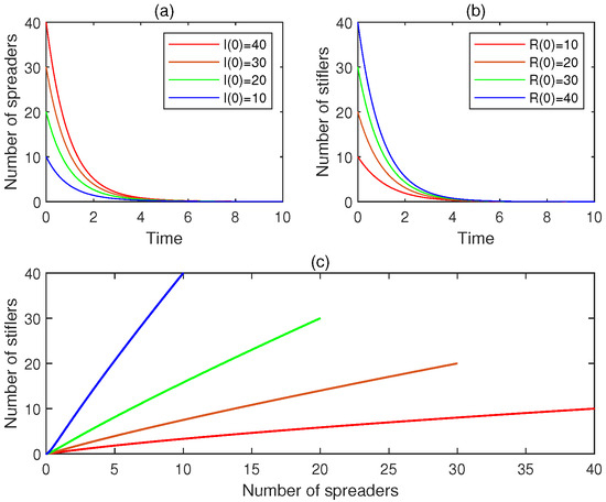 Figure 1. The experimental results for Experiment 1: (a) the four time plots for the number of spreaders, (b) the four time plots for the number of stiflers, and (c) the phase portrait. It is observed that the rumor-free equilibrium is locally asymptotically stable.
- Experiment 2. Consider model (3) with , , , , , , , and .
- -
- Since , it follows from claim (C2) of Theorem 3 that is unstable.
- -
- Consider the four initial conditions: , , , and . For , Figure 2a displays the time plot for , Figure 2b the time plot for . Additionally, Figure 2c portrays the associated phase portrait. It is observed that, for , does not approach zero. Hence, is unstable. This observation conforms to claim (C2) of Theorem 3.
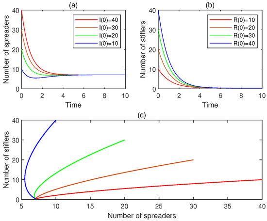 Figure 2. The experimental results for Experiment 2: (a) the four time plots for the number of spreaders, (b) the four time plots for the number of stiflers, and (c) the phase portrait. It is observed that the rumor-free equilibrium is unstable.
- Experiment 3. Consider model (3) with , , , , , and , , , and .
- -
- Since , it follows from claim (C1) of Theorem 4 that is locally asymptotically stable.
- -
- Consider the four initial conditions: , , , , and . For , Figure 3a depicts the time plot for . Figure 3b presents the time plot for . Additionally, Figure 3c shows the associated phase portrait. It is observed that, for , , . Hence, is locally asymptotically stable. This observation fits claim (C1) of Theorem 4.
 Figure 3. The experimental results for Experiment 3: (a) the four time plots for the number of spreaders, (b) the four time plots for the number of stiflers, and (c) the phase portrait. It is observed that the rumor-free equilibrium is locally asymptotically stable.
- Experiment 4. Consider model (3) with , , , , , , , , and .
- -
- Since , it follows from claim (C2) of Theorem 4 that is unstable.
- -
- Consider the four initial conditions: , , , , and . For , Figure 4a exhibits the time plot for , and Figure 4b displays the time plot for . Additionally, Figure 4c plots the associated phase portrait. It is observed that, for , does not approach zero. Hence, is unstable. This observation matches claim (C2) of Theorem 4.
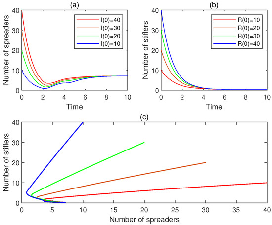 Figure 4. The experimental results for Experiment 4: (a) the four time plots for the number of spreaders, (b) the four time plots for the number of stiflers, and (c) the phase portrait. It is observed that the rumor-free equilibrium is unstable.
- Experiment 5. Consider model (3) with , , , , , , , and .
- -
- Since , it follows from Theorem 6 that is globally asymptotically stable.
- -
- Consider the four initial conditions: , , , and . For , Figure 5a depicts the time plot for . Figure 5b shows the time plot for . Additionally, Figure 5c exhibits the associated phase portrait. It is observed that, for , , . Hence, is globally asymptotically stable. This observation is consistent with Theorem 6.
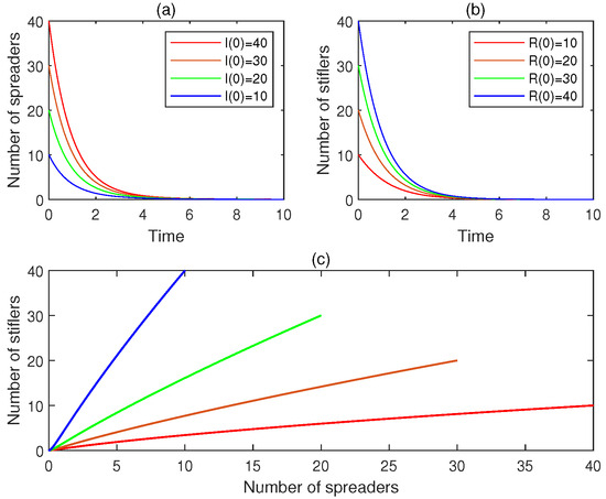 Figure 5. The experimental results for Experiment 5: (a) the four time plots for the number of spreaders, (b) the four time plots for the number of stiflers, and (c) the phase portrait. It is observed that the rumor-free equilibrium is globally asymptotically stable.
- Experiment 6. Consider model (3) with time delay, where , , , , , , , , and .
- -
- Since , it follows from Theorem 6 that is globally asymptotically stable.
- -
- Consider the four initial conditions: , , , , and . For , Figure 6a presents the time plot for . Figure 6b depicts the time plot for . Additionally, Figure 6c demonstrates the phase portrait. It is observed that, for , , . Hence, is globally asymptotically stable. This observation accords with Theorem 6.
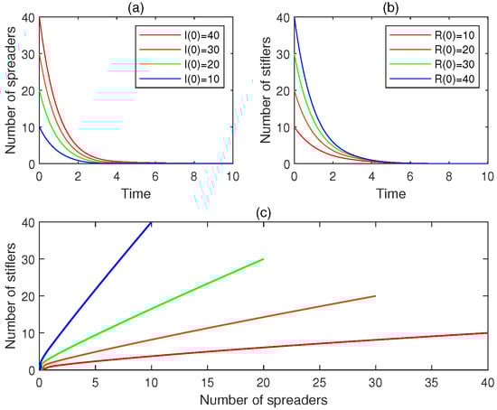 Figure 6. The experimental results for Experiment 6: (a) the four time plots for the number of spreaders, (b) the four time plots for the number of stiflers, and (c) the phase portrait. It is observed that the rumor-free equilibrium is globally asymptotically stable.
6.2. Asymptotic Stability of the Rumor-Endemic Equilibrium
- Experiment 7. Consider model (3) with , , , , , , , and .
- -
- is a rumor-endemic equilibrium.
- -
- Since , , , it follows from Theorem 7 that is locally asymptotically stable.
- -
- Consider the initial conditions: , , , , and . For , Figure 7a displays the time plot for . Figure 7b exhibits the time plots for . Figure 7c plots the phase portrait. It is observed that, for , , . Hence, is locally asymptotically stable. This observation is line with Theorem 7.
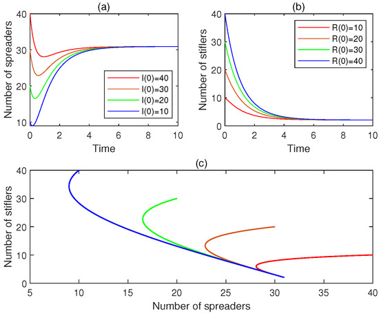 Figure 7. The experimental results for Experiment 7: (a) the four time plots for the number of spreaders, (b) the four time plots for the number of stiflers, and (c) the phase portrait. It is observed that the rumor-endemic equilibrium is locally asymptotically stable.
- Experiment 8. Consider model (3) with , , , , , , , and .
- -
- is a rumor-endemic equilibrium.
- -
- Since , , , it follows from Theorem 8 that is locally asymptotically stable.
- -
- Consider the four initial conditions: , , , , and . For , Figure 8a presents the time plot for . Figure 8b depicts the time plot for . Additionally, Figure 8c provides the phase portrait. It is observed that, for , , . Hence, is locally asymptotically stable. This observation conforms to Theorem 8.
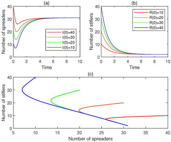 Figure 8. The experimental results for Experiment 8: (a) the four time plots for the number of spreaders, (b) the four time plots for the number of stiflers, and (c) the phase portrait for the state evolution. It is observed that the rumor-endemic equilibrium is locally asymptotically stable.
6.3. Effect of Time Delays
Under model (3), the effect of time delays on rumor-spreading is examined through numerical simulations.
- Experiment 9. Consider five delayed rumor-spreading models with , , , , , , , , and .
- -
- For each combination , consider the initial condition . Figure 9a exhibits the time plot for the number of spreaders, Figure 9b depicts the time plot for the number of stiflers, Figure 9c displays the time plot for the cumulative number of spreaders, and Figure 9d shows the time plot for the cumulative number of stiflers.
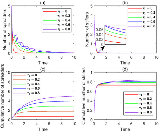 Figure 9. The experimental results for Experiment 9. For each combination of time delays, (a–d) exhibit the time plots for the number of spreaders, the number of stiflers, the number of cumulative spreaders, and the number of cumulative stiflers, respectively.
 - -
- The following phenomena are observed: (i) With the increase in , the number of spreaders is decreasing more slowly. (ii) With the increase in , the number of stiflers is decreasing more slowly. (iii) With the increase in , the cumulative number of spreaders is increasing more slowly. (iv) With the increase in , the cumulative number of stiflers is increasing more slowly.
- Experiment 10. Consider five delayed rumor-spreading models with , , , , , , , , and .
- -
- For , let , . For each combination , Figure 10a exhibits the time plot for the number of spreaders, Figure 10b depicts the time plot for the number of stiflers, Figure 10c displays the time plot for the cumulative number of spreaders, and Figure 10d shows the time plot for the cumulative number of stiflers.
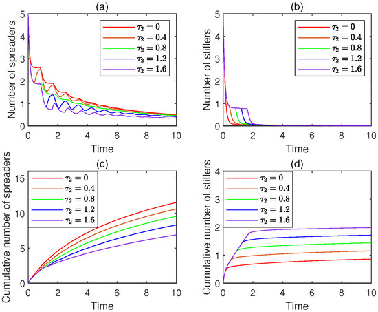 Figure 10. The experimental results for Experiment 10. For each combination of time delays, (a–d) exhibit the time plots for the number of spreaders, the number of stiflers, the number of cumulative spreaders, and the number of cumulative stiflers, respectively.
 - -
- The following phenomena are observed: (i) With the increase in , the number of spreaders is decreasing more slowly. (ii) With the increase in , the number of stiflers is decreasing more slowly. (iii) With the increase in , the cumulative number of spreaders is increasing more slowly. (iv) With the increase in , the cumulative number of stiflers is increasing more slowly.
From the above experiments and 1000 similar experiments, the following conclusions are drawn and explained:
- (a)
- With the increase in the first time delay, the number of spreaders is decreasing more slowly. The phenomenon can be explained in this way: with the increase in the first time delay, it takes longer time for an ignorant person to become rumor-spreading.
- (b)
- With the increase in the second time delay, the number of stiflers is decreasing more slowly. With the increase in the second time delay, it takes longer time for a spreader to become rumor-stifling.
- (c)
- With the increase in the first time delay, the cumulative number of spreaders is increasing more slowly. The explanation is similar to that of conclusion (a).
- (d)
- With the increase in the second time delay, the cumulative number of stiflers is increasing more slowly. The explanation is similar to that of conclusion (b).
7. Optimal Control of Delayed Rumor-Spreading
This section focuses on the problem of effectively controlling the spread of a rumor in the presence of two time delays and saturation effect.
7.1. A Delayed Optimal Control Model
The modeling of the original problem consists of three stages: In the first stage, a control function is introduced into the delayed rumor-spreading model (3) to form a controlled delayed rumor-spreading model. In the second stage, the cost used for carrying out a control function is estimated. In the third stage, an optimal control model for the original problem is formulated.
First, suppose a control function, denoted , will be carried out in the prespecified interval , with the goal of minimizing the negative impact of rumor-spreading. By introducing this control into model (3), a controlled delayed rumor-spreading model is formed, which is formulated as
Here, the term in the first equation characterizes the inhibition effect of on the number of spreaders, whereas the term in the second equation captures the promotion effect of on the number of stiflers.
Owing to the limited control cost, it may be reasonably assumed that u is bounded, i.e.,
Second, the cost needed by executing the control function can be divided into two sub-costs: the spread cost and the control cost. Here, the former refers to the negative impact caused by the propagation of the rumor, whereas the latter refers to the cost invested by the control.
The spread cost is proportional to the cumulative number of spreaders. Generally, the larger the cumulative number, the larger the impact of the rumor-spreading would be. Hence, the spread cost can be estimated to be
Generally, the control cost is assumed to be proportional to the cumulative quadratic function in . Hence, the control cost is estimated to be
Here, is a constant, and measures the running cost of realizing .
Consequently, the cost needed by executing the control function is estimated to be
In what follows, is taken to be our objective functional.
By combining the previous discussions, the original problem can be reduced to the following optimal control model:
7.2. Solution of the Delayed Optimal Control Model
In the preceding subsection, the delayed optimal control model (57) was established. The next task is to solve the model. The solution consists of four stages. In the first stage, the Lagrange and Hamiltonian for the model are established. In the second stage, the optimality system for the model is derived. In the third stage, an iterative algorithm for solving the model is presented. In the last stage, some controls are obtained by solving the optimality system.
First, it follows from optimal control theory [63] that the Lagrange for model (57) is
and the associated Hamiltonian is
where and represent the costate functions. For brevity, let
Second, let denote the characteristic function for the set X, i.e.,
For brevity, let
Let be an optimal control function and the associated state function. By Pontryagin Minimum Principle [63], there exist costate functions and such that
Additionally, it follows from Pontryagin Minimum Principle [63] that there is a control function such that
Through clamping, it follows that
Suppose there is no boundary constraint. The optimality system for model (57) is given by
Next, model (57) can be solved by applying the Forward–Backward Sweep Method [64] to the optimality system (66). Below, the procedure is presented.
Initialization.
- (1)
- Set a small positive number , say .
- (2)
- Let , , . Let .
- (3)
- Let . Choose an initial control so that , .
Iterations.
- (4)
- Let .
- (5)
- Use Equations (52) with to forwardly calculate and , resulting in a pair of state functions, denoted and .
- (6)
- Use Equation (63) with , , and to backwardly calculate and , resulting in a pair of costate functions, denoted and .
- (7)
- Use Equations (64) and (65) with , , , and to calculate , resulting in a control, denoted .
- (8)
- If , output . Otherwise, return step (4).
In the situation where the iteration converges, an admissible control is obtained. For convenience, this control is referred to as a good control.
Remark 2.
It is empirically found that, when and are relatively small, the iterations always converge.
Finally, some good controls are obtained through simulation experiments.
- Experiment 11. Consider model (57) with , , , , , , , , , , , and . For , let .
- (i)
- By applying the Forward–Backward Sweep Method, a good control, denoted , is obtained. Figure 11a exhibits .
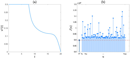 Figure 11. The experimental results for Experiment 11: (a) the good control . (b) versus u, .
 - (ii)
- For comparative purposes, a set of 100 controls, denoted , are generated randomly. Figure 11b displays versus u, . It is observed that the cost of is significantly lower than the costs of all the remaining controls. Hence, is satisfactory in terms of the cost.
- Experiment 12. Consider model (57) with , , , , , , , , , , , and . For , let .
- (i)
- By applying the Forward–Backward Sweep Method, a good control, denoted , is obtained. Figure 12a exhibits .
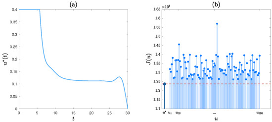 Figure 12. The experimental results for Experiment 12: (a) the control . (b) versus u, .
 - (ii)
- For comparative purposes, a set of 100 controls, denoted , are generated randomly. Figure 12b displays versus u, . It is observed that the cost of is significantly lower than the costs of all the remaining controls. Hence, is satisfactory in terms of the cost.
From these two experiments and a thousand similar experiments, it is concluded that the good control is satisfactory in terms of the cost.
7.3. Effect of Time Delays
This subsection examines the effect of the two time delays on the cost of the good control through simulation experiments.
- Experiment 13. Consider a set of models (57) with , , , , , , , , , , , and . For , let .
- (i)
- By applying the Forward–Backward Sweep Method, a set of good controls, denoted , are obtained.
- (ii)
- Figure 13 displays versus , . It is observed that is decreasing with the increase in .
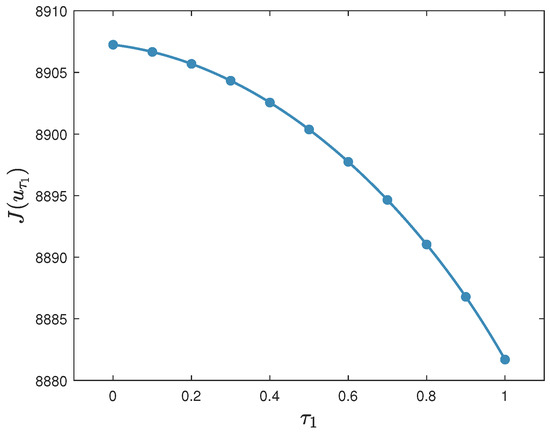 Figure 13. The experimental results for Experiment 13: versus , .
- Experiment 14. Consider a set of models (57) with , , , , , , , , , , , and . For , let .
- (i)
- By applying the Forward–Backward Sweep Method, a set of good controls, denoted , are obtained.
- (ii)
- Figure 14 displays versus , . It is observed that is increasing with the increase in .
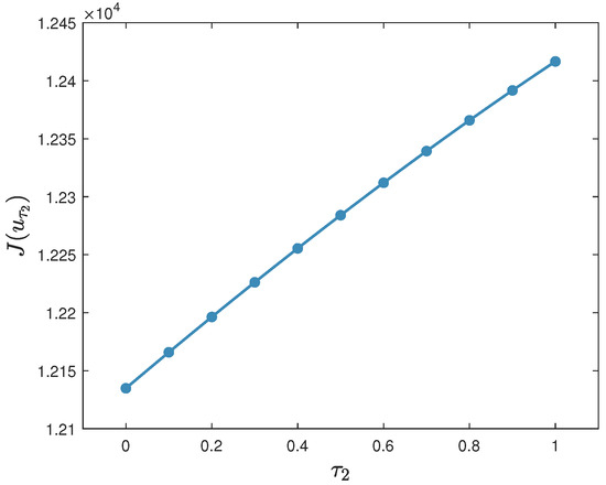 Figure 14. The experimental results for Experiment 15: versus , .
From these two experiments and a thousand similar experiments, the following conclusions are drawn and explained:
- (a)
- The cost of the good control is decreasing with the increase in the first time delay. This phenomenon can be explained in this way: with the increase in the first time delay, it takes longer time for an ignorant person to become rumor-spreading. So, the cumulative number of spreaders decreases. Hence, the cost of the good control declines.
- (b)
- The cost of the good control is increasing with the increase in the second time delay. The phenomenon can be explained in this way: with the increase in the second time delay, it takes longer time for a spreader to become rumor-stifling. So, the cumulative number of spreaders increases. Hence, the cost of the good control increases.
8. Conclusions
In this article, a rumor-spreading model with two unequal time delays and a saturation effect has been proposed. A complex bifurcation phenomenon has been revealed. A collection of criteria for the asymptotic stability of the rumor-free equilibrium have been presented. In the absence of a time delay or in the presence of small time delays, a criterion for the local asymptotic stability of the rumor-endemic equilibrium has been presented. An optimal control model for restraining the spread of a rumor has been formulated and resolved. This work contributes to the understanding of the dynamics of rumor-spreading models with unequal time delays.
Several relevant issues are worth further investigation. First, although there are a number of publicly available rumor datasets [65,66], there is currently no publicly available dataset that is closely related to rumor-spreading. For the purpose of justifying a delayed rumor-spreading model, it is imperative to construct a dataset that is closely related to delayed rumor-spreading. Second, this article considers a rumor-spreading model with two distinct time delays. In the real world, there may exist more than two distinct time delays. Consequently, it is valuable to establish and study complex delayed rumor-spreading models. Next, the saturation effect of rumor-spreading or rumor-stifling is a characteristic feature of rumor-spreading. To date, most delayed rumor-spreading models are of the most simple Holling type II [29,41,42,43,44,45,46,47,48,49,50,51,52,53,54]. In practice, a delayed rumor-spreading model may be of some other type [55]. Consequently, it is worthwhile to consider delayed rumor-spreading models with more complex saturation effects [33,34,35,36,37,38]. Finally, the confrontation between a rumormonger and the associated rumor-refuter is essentially a non-cooperative game [67]. Consequently, the research of rumor-spreading in the framework of game theory is of practical importance [18].
Author Contributions
Funding acquisition, C.W. and C.F.; investigation, C.F., X.Y. and Y.Q.; validation, C.W. and X.Y.; writing—original draft preparation, X.Y.; writing—review and editing, L.Y. All authors have read and agreed to the published version of the manuscript.
Funding
This research was funded by the Opening Foundation of the State Key Laboratory of Cognitive Intelligence, grant number iFLYTEK [COGOS-2024HE03].
Data Availability Statement
The original contributions presented in this study are included in the article. Further inquiries can be directed to the corresponding author.
Conflicts of Interest
The authors declare no conflicts of interest.
References
- Peterson, W.; Gist, N.P. Rumor and public opinion. Am. J. Sociol. 1951, 57, 159–167. [Google Scholar] [CrossRef]
- Allport, G.W.; Postman, L. An analysis of rumor. Public Opin. Q. 1946, 10, 501–517. [Google Scholar] [CrossRef]
- Britton, N.F. Essential Mathematical Biology; Springer: Berlin/Heidelberg, Germany, 2003. [Google Scholar]
- Goffman, W.; Newill, V.A. Generalization of epidemic Theory: An application to the transmission of ideas. Nature 1964, 204, 501–517. [Google Scholar] [CrossRef]
- Daley, D.J.; Kendall, D.G. Epidemics and rumours. Nature 1964, 204, 1118. [Google Scholar] [CrossRef] [PubMed]
- Daley, D.J.; Kendall, D.G. Stochastic rumours. IMA J. Appl. Math. 1965, 1, 42–55. [Google Scholar] [CrossRef]
- Zhao, L.; Wang, J.; Chen, Y.; Wang, Q.; Cheng, J.J.; Cui, H. SIHR rumor spreading model in social networks. Phys. A 2012, 391, 2444–2453. [Google Scholar] [CrossRef]
- Wang, J.; Zhao, L.; Huang, R. 2SI2R rumor spreading model in homogeneous networks. Phys. A 2014, 413, 153–161. [Google Scholar] [CrossRef]
- Zhao, L.; Wang, X.; Wang, J.; Qiu, X.; Xie, W. Rumor-propagation model with consideration of refutation mechanism in homogeneous social networks. Discret. Dyn. Nat. Soc. 2014, 1, 659273. [Google Scholar] [CrossRef]
- Wei, Y.; Huo, L.; He, H. Research on rumor-spreading model with Holling type III functional response. Mathematics 2022, 10, 632. [Google Scholar] [CrossRef]
- Huo, L.; Ding, F.; Liu, C.; Cheng, Y. Dynamical analysis of rumor spreading model considering node activity in complex networks. Complexity 2018, 1, 1049805. [Google Scholar] [CrossRef]
- Huo, L.; Chen, S. Rumor propagation model with consideration of scientific knowledge level and social reinforcement in heterogeneous network. Physica 2020, 559, 125063. [Google Scholar] [CrossRef]
- Huo, L.; Chen, S.; Xie, X.; Liu, H.; He, J. Optimal control of ISTR rumor propagation model with social reinforcement in heterogeneous network. Complexity 2021, 1, 5682543. [Google Scholar] [CrossRef]
- Tong, X.; Jiang, H.; Chen, X.; Yu, S.; Li, J. Dynamic analysis and optimal control of rumor spreading model with recurrence and individual behaviors in heterogeneous networks. Entropy 2022, 24, 464. [Google Scholar] [CrossRef] [PubMed]
- Yang, L.X.; Li, P.; Yang, X.; Wu, Y.; Tang, Y.Y. On the competition of two conflicting messages. Nonlinear Dyn. 2018, 91, 1853–1869. [Google Scholar] [CrossRef]
- Yang, L.X.; Zhang, T.; Yang, X.; Wu, Y.; Tang, Y.Y. Effectiveness analysis of a mixed rumor-quelling strategy. J. Frankl. Inst. 2018, 355, 8079–8105. [Google Scholar] [CrossRef]
- Zhao, J.; Yang, L.X.; Zhong, X.; Yang, X.; Wu, Y.; Tang, Y.Y. Minimizing the impact of a rumor via isolation and conversion. Physica 2019, 526, 120867. [Google Scholar] [CrossRef]
- Huang, D.W.; Yang, L.X.; Li, P.; Yang, X.; Tang, Y.Y. Developing cost-effective rumor-refuting strategy through game-theoretic approach. IEEE Syst. J. 2021, 15, 5034–5045. [Google Scholar] [CrossRef]
- Long, X.; Gong, S. New results on stability of Nicholson’s blowflies equation with multiple pairs of time-varying delays. Appl. Math. Lett. 2020, 100, 106027. [Google Scholar] [CrossRef]
- Huang, C.; Liu, B. Traveling wave fronts for a diffusive Nicholson’s blowflies equation accompanying mature delay and feedback delay. Appl. Math. Lett. 2022, 134, 108321. [Google Scholar] [CrossRef]
- Huang, C.; Liu, B. Exponential stability of a diffusive Nicholson’s blowflies equation accompanying multiple time-varying delays. Appl. Math. Lett. 2025, 163, 109451. [Google Scholar] [CrossRef]
- Zhu, L.; Zhou, M.; Zhang, Z. Dynamical analysis and control strategies of rumor spreading models in both homogeneous and heterogeneous networks. J. Nonlinear Sci. 2020, 30, 2545–2576. [Google Scholar] [CrossRef]
- Dong, Y.; Huo, L.; Zhao, L. An improved two-layer model for rumor propagation considering time delay and event-triggered impulsive control strategy. Chaos Solitons Fractals 2022, 164, 112711. [Google Scholar] [CrossRef]
- Guo, H.; Yan, X.; Niu, Y.; Zhang, J. Dynamic analysis of rumor propagation model with media report and time delay on social networks. J. Appl. Math. Comput. 2023, 69, 2473–2502. [Google Scholar] [CrossRef] [PubMed]
- Luo, X.; Jiang, H.; Li, J.; Chen, S.; Xia, Y. Modeling and controlling delayed rumor propagation with general incidence in heterogeneous networks. Int. J. Mod. Phys. C 2024, 35, 2450020. [Google Scholar] [CrossRef]
- Ghosh, M.; Das, P. Analysis of online misinformation spread model incorporating external noise and time delay and control of media effort. Differ. Equ. Dyn. Syst. 2025, 33, 261–301. [Google Scholar] [CrossRef]
- Cheng, Y.; Huo, L.; Zhao, L. Dynamical behaviors and control measures of rumor-spreading model in consideration of the infected media and time delay. Inf. Sci. 2021, 564, 237–253. [Google Scholar] [CrossRef]
- Cheng, Y.; Huo, L.; Zhao, L. Stability analysis and optimal control of rumor spreading model under media coverage considering time delay and pulse vaccination. Chaos Solitons Fractals 2022, 157, 111931. [Google Scholar] [CrossRef]
- Fu, C.; Liu, G.; Yang, X.; Qin, Y.; Yang, L. A Rumor-Spreading Model with Three Identical Time Delays. Mathematics 2025, 13, 1421. [Google Scholar] [CrossRef]
- Avila-Vales, E.; Perez, A.G.C. Dynamics of a time-delayed SIR epidemic model with logistic growth and saturated treatment. Chaos Solitons Fractals 2019, 127, 55–69. [Google Scholar] [CrossRef]
- Kumar, A.; Nilam. Stability of a delayed SIR epidemic model by introducing two explicit treatment classes along with nonlinear incidence rate and holling type treatment. Comput. Appl. Math. 2019, 38, 130. [Google Scholar] [CrossRef]
- Goel, K.; Kumar, A.; Nilam. A deterministic time-delayed SVIRS epidemic model with incidences and saturated treatment. J. Eng. Math. 2020, 121, 19–38. [Google Scholar] [CrossRef]
- Kumar, A.; Nilam. Effects of nonmonotonic functional responses on a disease transmission model: Modeling and simulation. Commun. Math. Stat. 2021, 10, 195–214. [Google Scholar] [CrossRef] [PubMed]
- Kumar, A.; Nilam. Mathematical analysis of a delayed epidemic model with nonlinear incidence and treatment rates. J. Eng. Math. 2019, 115, 1–20. [Google Scholar] [CrossRef]
- Goel, K.; Nilam. Stability behavior of a nonlinear mathematical epidemic transmission model with time delay. Nonlinear Dyn. 2019, 98, 1501–1518. [Google Scholar] [CrossRef]
- Goel, K.; Nilam. A mathematical and numerical study of a SIR epidemic model with time delay, nonlinear incidence and treatment rates. Theory Biosci. 2019, 138, 203–213. [Google Scholar] [CrossRef]
- Fatini, M.E.; Sekkak, I.; Laaribi, A. A threshold of a delayed stochastic epidemic model with Crowly-Martin functional response and vaccination. Phys. A 2019, 520, 151–160. [Google Scholar] [CrossRef]
- Upadhyay, R.K.; Pal, A.K.; Kumari, S.; Roy, R. Dynamics of an SEIR epidemic model with nonlinear incidence and treatment rates. Nonlinear Dyn. 2019, 96, 2351–2368. [Google Scholar] [CrossRef]
- Huo, L.; Ma, C. Optimal control of rumor spreading model with consideration of psychological factors and time delay. Discret. Dyn. Nat. Soc. 2018, 2018, 9314907. [Google Scholar] [CrossRef]
- Huo, L.; Jiang, J.; Gong, S.; He, B. Dynamical behavior of a rumor transmission model with Holling-type II functional response in emergency event. Phys. A Stat. Mech. Its Appl. 2016, 450, 228–240. [Google Scholar] [CrossRef]
- Li, C. A study on time-delay rumor propagation model with saturated control function. Adv. Differ. Equ. 2017, 2017, 255. [Google Scholar] [CrossRef]
- Zhu, L.; Zhao, H. Dynamical behaviours and control measures of rumour-spreading model with consideration of network topology. Int. J. Syst. Sci. 2017, 48, 2064–2078. [Google Scholar] [CrossRef]
- Zhu, L.; Guan, G. Dynamical analysis of a rumor spreading model with self-discrimination and time delay in complex networks. Phys. A 2019, 533, 121953. [Google Scholar] [CrossRef]
- Zhu, L.; Huang, X. SIS model of rumor spreading in social network with time delay and nonlinear functions. Commun. Theor. Phys. 2020, 72, 015002. [Google Scholar] [CrossRef]
- Zhu, L.; Liu, W.; Zhang, Z. Delay differential equations modeling of rumor propagation in both homogeneous and heterogeneous networks with a forced silence function. Appl. Math. Comput. 2020, 370, 124925. [Google Scholar] [CrossRef]
- Huo, L.; Chen, X. Dynamical analysis of a stochastic rumor-spreading model with Holling II functional response function and time delay. Adv. Differ. Equ. 2020, 2020, 651. [Google Scholar] [CrossRef]
- Wang, J.; Jiang, H.; Hu, C.; Yu, Z.; Li, J. Stability and Hopf bifurcation analysis of multi-lingual rumor spreading model with nonlinear inhibition mechanism. Chaos Solitons Fractals 2021, 153, 111464. [Google Scholar] [CrossRef]
- Yue, X.; Huo, L. Analysis of the stability and optimal control strategy for an ISCR rumor propagation model with saturated incidence and time delay on a scale-free network. Mathematics 2022, 10, 3900. [Google Scholar] [CrossRef]
- Ghosh, M.; Das, S.; Das, P. Dynamics and control of delayed rumor propagation through social networks. J. Appl. Math. Comput. 2022, 68, 3011–3040. [Google Scholar] [CrossRef]
- Yu, S.; Yu, Z.; Jiang, H. Stability, Hopf bifurcation and optimal control of multilingual rumor-spreading model with isolation mechanism. Mathematics 2022, 10, 4556. [Google Scholar] [CrossRef]
- Yuan, T.; Guan, G.; Shen, S.; Zhu, L. Stability analysis and optimal control of epidemic-like transmission model with nonlinear inhibition mechanism and time delay in both homogeneous and heterogeneous networks. J. Math. Anal. Appl. 2023, 526, 127273. [Google Scholar] [CrossRef]
- Cao, B.; Guan, G.; Shen, S.; Zhu, L. Dynamical behaviors of a delayed SIR information propagation model with forced silence function and control measures in complex networks. Eur. Phys. J. Plus 2023, 138, 402. [Google Scholar] [CrossRef] [PubMed]
- Ma, Y.; Xie, L.; Liu, S.; Chu, X. Dynamical behaviors and event-triggered impulsive control of a delayed information propagation model based on public sentiment and forced silence. Eur. Phys. J. Plus 2023, 138, 979. [Google Scholar] [CrossRef]
- Ding, N.; Guan, G.; Shen, S.; Zhu, L. Dynamical behaviors and optimal control of delayed S2IS rumor propagation model with saturated conversion function over complex networks. Commun. Nonlinear Sci. Numer. Simul. 2024, 128, 107603. [Google Scholar] [CrossRef]
- Li, C.; Ma, Z. Dynamics analysis and optimal control for a delayed rumor-spreading model. Mathematics 2022, 10, 3455. [Google Scholar] [CrossRef]
- Xiao, D.; Ruan, S. Global analysis of an epidemic model with nonmonotone incidence rate. Math. Biosci. 2007, 208, 419–429. [Google Scholar] [CrossRef]
- Buonomo, B.; Rionero, S. On the Lyapunov stability for SIRS epidemic models with general nonlinear incidence rate. Appl. Math. Comput. 2010, 217, 4010–4016. [Google Scholar] [CrossRef]
- Diekmann, O.; Heesterbeek, J.A.P.; Metz, J.A.J. On the definition and the computation of the basic reproduction ratio R0 in models for infectious diseases in heterogeneous populations. J. Math. Biol. 1990, 28, 365–382. [Google Scholar] [CrossRef]
- van den Driessche, P.; Watmough, J. Reproduction numbers and sub-threshold endemic equilibria for compartmental models of disease transmission. Math. Biosci. 2002, 180, 29–48. [Google Scholar] [CrossRef]
- Robinson, R.K. An Introduction to Dynamical Systems: Continuous and Discrete, 2nd ed.; American Mathematical Society: Providence, RI, USA, 2012. [Google Scholar]
- Wei, H.; Li, X.; Martcheva, M. An epidemic model of a vector-borne disease with direct transmission and time delay. J. Math. Anal. Appl. 2008, 342, 895–908. [Google Scholar] [CrossRef]
- Ruan, S.; Wei, J. On the zeros of transcendental functions with applications to stability of delay differential equations with two delays. Dyn. Contin. Discret. Impuls. Syst. 2003, 10, 863–874. [Google Scholar]
- Kirk, D.E. Optimal Control Theory: An Introduction; Dover Publications: Mineola, NY, USA, 2004. [Google Scholar]
- McAsey, M.; Mou, L.; Han, W. Convergence of the forward-backward sweep method in optimal control. Comput. Optim. Appl. 2012, 53, 207–226. [Google Scholar] [CrossRef]
- Li, Q.; Zhang, Q.; Si, L.; Liu, Y. Rumor detection on social media: Datasets, methods and opportunities. In Proceedings of the Second Workshop on Natural Language Processing for Internet Freedom: Censorship, Disinformation, and Propaganda, Hong Kong, China, 4 November 2019. [Google Scholar]
- Nasser, M.; Arshad, N.I.; Ali, A.; Alhussian, H.; Saeed, F.; Da’u, A.; Nafea, I. A systematic review of multimodal fake news detection on social media using deep learning models. Results Eng. 2025, 26, 104752. [Google Scholar] [CrossRef]
- Owen, G. Game Theory; Emerald Group Pub Ltd.: Leeds, UK, 2013. [Google Scholar]
Disclaimer/Publisher’s Note: The statements, opinions and data contained in all publications are solely those of the individual author(s) and contributor(s) and not of MDPI and/or the editor(s). MDPI and/or the editor(s) disclaim responsibility for any injury to people or property resulting from any ideas, methods, instructions or products referred to in the content. |
© 2025 by the authors. Licensee MDPI, Basel, Switzerland. This article is an open access article distributed under the terms and conditions of the Creative Commons Attribution (CC BY) license (https://creativecommons.org/licenses/by/4.0/).