Advanced Vehicle Routing for Electric Fleets Using DPCGA: Addressing Charging and Traffic Constraints

Abstract

With the rapid proliferation of electric vehicles (EVs), urban logistics faces increasing challenges in optimizing vehicle routing. This paper presents a new modeling framework for the Electric Vehicle Routing Problem (EVRP), where multiple electric trucks serve a set of customers within their capacity limits. The model incorporates critical EV-specific constraints, including limited battery range, charging demand, and dynamic urban traffic conditions, with the objective of minimizing total delivery cost. To efficiently solve this problem, a Dual Population Cooperative Genetic Algorithm (DPCGA) is proposed. The algorithm employs a dual-population mechanism for global exploration, effectively expanding the search space and accelerating convergence. It then introduces local refinement operators to improve solution quality and enhance population diversity. A large number of experimental results demonstrate that DPCGA significantly outperforms traditional algorithms in terms of performance, achieving an average 3% improvement in customer satisfaction and a 15% reduction in computation time. Furthermore, this algorithm shows superior solution quality and robustness compared to the AVNS and ESA-VRPO algorithms, particularly in complex scenarios such as adjustments in charging station layouts and fluctuations in vehicle range. Sensitivity analysis further verifies the stability and practicality of DPCGA in real-world urban delivery environments.

1. Introduction

In recent years, with the acceleration of global economic integration and urbanization, the transportation industry has been facing unprecedented challenges. Particularly in the context of meeting the growing logistics demand and achieving environmental goals, transportation optimization issues have garnered widespread attention. Since its introduction in the 1950s, the Vehicle Routing Problem (VRP) has become one of the classic combinatorial optimization problems. The objective of VRP is to minimize transportation costs, time, or other related objectives by reasonably planning the routes of a fleet of delivery vehicles, while satisfying constraints such as vehicle capacity, delivery time windows, and others. VRP has broad applications in various fields, including logistics distribution and traffic management.

With the rapid development of electric vehicles (EVs) and the strengthening of global environmental policies, electric vehicles have gradually become an important component of modern transportation systems. Many countries have implemented policies to promote the widespread adoption of electric vehicles, aiming to reduce greenhouse gas emissions, decrease reliance on fossil fuels, and encourage green travel. These policies have not only facilitated the transformation of the traditional automobile industry but have also played a positive role in urban delivery, logistics, and other fields, particularly in reducing carbon emissions and optimizing resource allocation.

The Electric Vehicle Routing Problem (EVRP) is an extension of the Vehicle Routing Problem (VRP), incorporating unique constraints such as battery range, charging requirements, and charging station layout. Unlike the traditional VRP, EVRP must consider factors such as the selection of charging stations, charging time, and the layout of charging facilities, significantly increasing the complexity of the route planning. To ensure that electric vehicles can successfully complete their tasks, the route planning must balance the efficiency of charging point selection and charging time.

1.1. Literature Review

In recent years, many researchers have proposed innovative strategies to address the challenges in electric vehicle path planning. For instance, Rupnik et al. [1] proposed a hybrid model for electric vehicles that addresses charging demands and range issues; El Wafi et al. [2] introduced a dynamic path planning method based on reinforcement learning, which can adjust routes based on real-time traffic and charging demands. These studies have provided valuable insights for the theoretical development of electric vehicle path planning and the layout of charging stations.

With the development of big data and Internet of Things technologies, Han and Guo [3] proposed an electric vehicle path planning method based on big data analysis, which optimizes electric vehicle scheduling and charging resource allocation by integrating real-time traffic data, charging station load, and user behavior. The combination of these technologies has significantly improved the efficiency of electric vehicle path planning, particularly in complex urban environments, enabling more efficient traffic management and charging resource allocation [4]. Moreover, with the growth of the electric vehicle market, the multi-vehicle collaborative path planning problem has also gradually gained attention.

At the same time, researchers have conducted interdisciplinary explorations in the field of electric vehicle path planning, introducing many new elements. For example, Sun et al. [5] proposed a bus trajectory-based street center routing strategy that optimizes message delivery efficiency in VANETs by combining fixed bus routes and trajectory characteristics. They also introduced an intersection fog computing-based routing strategy, which optimizes path selection errors caused by traffic flow and road condition changes by introducing dynamic fog nodes [6]. Furthermore, Sun et al. [7] further studied the use of relay nodes from parked vehicles, proposing an ARIMA model that provides a robust solution for inter-vehicle communication paths in dynamic urban environments, significantly improving network stability and communication quality. Additionally, Xiao et al. [8] proposed a conditional anonymity and anti-leakage authentication scheme for vehicular crowdsourcing communication, ensuring data privacy and enhancing communication security and reliability.

Overall, researchers have achieved optimizations and improvements in strategies, algorithms, and other aspects of path planning, integrating excellent methods from other fields. Many innovative outcomes have been achieved, providing us with valuable insights and promoting the formation and optimization of our own strategies. However, for increasingly complex path planning problems, which often involve many dynamic factors, despite the numerous innovative achievements, there are still issues in practical applications, such as incomplete consideration of strategies and insufficient applicability of algorithms. How to improve the solving efficiency of algorithms, enhance the ability to handle complex constraints, and effectively respond to dynamic environmental changes remains a key challenge in current research. Next, we will focus on discussing some of the path planning strategies and algorithms from the literature, along with their applications and improvements in addressing these challenges.

First, regarding strategies, most of the literature focuses on traditional path planning problems, often considering constraints related to refueling stations, where refueling time is typically neglected. However, for electric vehicle problems, the charging time of vehicles is relatively long and cannot be ignored, significantly increasing the complexity of the problem. Moreover, a large portion of the literature focuses on single-vehicle scenarios, specifically for single-vehicle deliveries. There is also an issue of oversimplification in the literature, where speed is assumed to be constant, simplifying the problem but making it less consistent with real-world conditions and reducing its rigor. For example, the hybrid planning strategy proposed by Gaon et al. [9] improves convergence speed, but its adaptability to constraints such as charging station layout and battery range is relatively poor. The bi-level programming method improved by Gan et al. [10] makes breakthroughs in global search and balances multi-objective problems well. However, it significantly simplifies constraint handling, and issues such as long computation times and slow convergence still exist when dealing with large-scale complex constraints, real-time traffic flow, and frequently changing charging demands.

In contrast, the strategy presented in this paper is more comprehensive. This paper considers charging stations and user locations, incorporates charging time, and combines multiple factors such as time windows and time-varying speeds, making it more consistent with real-world conditions. It also establishes multiple optimization objectives, such as maximizing user satisfaction and minimizing time cost, travel cost, and penalty costs. These are then treated as a single objective and transformed into a single-objective optimization problem. This makes the optimization goal more comprehensive while reducing the optimization difficulty. Additionally, beyond the single-vehicle scenario, this paper also considers multi-vehicle delivery, expanding the scope beyond a single research object and significantly enhancing the completeness of the strategy.

However, with the strategy being more comprehensive, it presents significant challenges at the algorithmic level. The problem becomes more complex, and the optimization difficulty increases. Traditional algorithms are not well suited to handle our problem. The following discusses and reflects on the algorithms presented in the literature, as well as an introduction to the algorithm proposed in this paper.

Liu et al. [11] proposed an improved Particle Swarm Optimization (PSO) algorithm, offering new insights into three-dimensional path planning problems. By introducing a time factor, they enhanced the convergence speed and accuracy of PSO, particularly in high-dimensional solution space searches, where it accelerates convergence and reduces computation time. This method makes PSO more adaptable to dynamically changing path planning tasks, especially in situations with significant real-time traffic and environmental condition changes, demonstrating strong adaptability and flexibility. It provides an important reference for addressing dynamic traffic and charging demand issues in electric vehicle path planning.

Xiao et al. [12] improved the Simulated Annealing algorithm and successfully applied it to the omnichannel vehicle routing problem. By enhancing global search capability, they avoided local optima, thus improving the reliability of path planning. The improved Simulated Annealing algorithm can effectively balance multiple objectives in optimization problems, making it particularly suitable for handling complex constraint conditions, demonstrating strong adaptability and efficiency.

Chen et al. [13] improved the Whale Optimization Algorithm, providing a new solution for robotic path planning. This algorithm improves the accuracy and convergence speed by optimizing the convergence mechanism, especially in high-dimensional solution spaces, where it effectively avoids local optima. The innovation lies in improving path planning accuracy, particularly in dynamic environments, where it significantly enhances the accuracy and efficiency of path selection.

1.2. Research Innovations

In the field of path optimization, the algorithms in the aforementioned literature have demonstrated certain advantages in finding the optimal path. However, when addressing core issues in electric vehicle path planning, problems such as slow local convergence, strong dependency on initial solutions, and insufficient adaptability to dynamic environments still exist. To address these issues, this paper proposes an improved Dual-Population Genetic Algorithm (DPCGA). Based on the dual-population GA, DPCGA has been optimized and has achieved significant results. The dual-population genetic algorithm with dynamic weights effectively handles changes in dynamic traffic flow, improving the accuracy and efficiency of electric vehicle path planning [14]. This method enhances the path optimization capability of DPCGA under time-varying constraints by incorporating time factors, making it particularly suitable for scenarios with significant fluctuations in real-time traffic and charging demands.

Additionally, DPCGA has been optimized through the adjustment of adaptive population ratios and has been widely applied to multi-objective optimization problems [15]. This strategy adjusts the ratio of elite population to exploratory population, balancing the optimization weights between different objectives, allowing DPCGA to simultaneously optimize multiple objectives and effectively balance trade-offs between them, thereby improving the overall operational efficiency of the system. Similar improvement methods have also been applied to Autonomous Underwater Vehicle path planning [16], successfully achieving efficient path searching and task scheduling for underwater robots in complex environments.

Furthermore, researchers have proposed combining DPCGA with a chaotic local search strategy to enhance the algorithm’s ability to handle large-scale optimization problems [17]. By introducing chaotic sequences, the diversity of local search is increased, avoiding the early convergence problems that may occur in traditional GA. With this combination, DPCGA can accelerate convergence when dealing with complex constraints and large-scale problems, avoid getting stuck in local optima, and converge more quickly to the global optimum.

Although methods based on dual-population genetic algorithms have achieved some success in traditional path planning, in electric vehicle path planning, they still face challenges from key constraints such as charging station layout, battery range, and charging demand. Existing strategies often struggle to meet the requirements for real-time response and high-precision optimization in electric vehicle path planning. The improved Dual-Population Genetic Algorithm (DPCGA) proposed in this paper effectively addresses these issues. It not only optimizes traditional path planning but also specifically considers factors such as charging station layout, battery range, and recipient addresses. Through the dual-population collaborative mechanism, DPCGA can optimize path planning under the constraints of charging station selection and battery range, ensuring that electric vehicles efficiently complete delivery tasks while charging quickly. Compared to traditional algorithms, DPCGA demonstrates stronger adaptability and advantages in handling multiple constraints and responding to dynamic changes in electric vehicle path planning. Therefore, DPCGA provides a more efficient and accurate solution for electric vehicle path planning, overcoming the limitations of traditional algorithms in the path planning of new energy vehicles.

Additionally, in the traditional VRPTW model, the customer satisfaction function strictly depends on the time window range, meaning that customer satisfaction is 100% only when the delivery occurs within the time window; otherwise, it is 0. However, this setting is too strict and does not account for the impact of road speed limits on delivery costs and customer satisfaction. To address this, this paper proposes a new model based on VRPTW—the Vehicle Routing Problem with Time Windows, Time-Varying Speeds, and Customer Satisfaction (VRP-TWTVS-CS). In this model, we use a more realistic fuzzy trapezoidal function to describe customer satisfaction and introduce road speed limits for different time periods, thereby better simulating real-world urban delivery environments. These improvements provide decision-makers with more options and richer decision insights, ultimately achieving the goal of improving delivery efficiency, reducing delivery costs, and enhancing customer satisfaction. Specifically, the main contributions of this paper are as follows:

• Based on the existing VRPTW mathematical model in the literature, a VRP-TWTVS-CS planning model is established.
• An improved dual-population genetic algorithm is used, setting elite populations and exploratory populations, introducing a dual-population collaborative development mechanism, and using a roulette wheel selection population to assist the development of the tournament selection population, thereby improving the algorithm and optimizing the solution speed and strengthening the algorithm’s solving ability.
• The VRP-TWTVS-CS model used in this paper and the DPCGA algorithm ultimately improved customer satisfaction by 3% on average compared to the ESA-VRPO and AVNS algorithms in customer satisfaction evaluation, reduced convergence time by 15%, and found better solutions in complex scenarios. This indicates that in real-world environments, service quality and customer satisfaction can be effectively improved.
• The effectiveness of the proposed algorithm was validated through two experiments, one of which used a dataset from the existing literature, and the other was adapted from the Solomon dataset, covering three different scale scenarios with a total of 15 instances.

1.3. Article Composition

The remaining structure of this paper is organized as follows. Section 2 will provide a detailed introduction to the model-building process for the VRP studied, along with an explanation of relevant assumptions, symbols, and model details. Section 3 focuses on the DPCGA algorithm we proposed, providing a detailed explanation of the key parameters in the algorithm. Section 4 presents the experimental results, which include two different experimental sections to validate the effectiveness and superiority of the algorithm. Section 5 explores the impact of factors such as range and the number of charging stations on the final results from the perspective of sensitivity analysis, providing a more detailed view for model optimization. Section 6 summarizes our research findings and proposes future research directions, offering reference and suggestions for further optimization and practical application.

2. Model Formulation

2.1. VRP-TWTVS-CS Model

This paper presents a vehicle routing model with time Windows, time-varying speeds, and customer satisfaction (VRP-TWTVS-CS) designed to constrain vehicle travel paths based on time windows, time-varying speeds, and customer satisfaction. The objective of the model is to optimize delivery paths, ensuring that vehicle speeds and arrival times maximize customer satisfaction while meeting customer demands. The model incorporates dynamic time-varying speed and precise time window constraints, allowing for fine control over vehicle travel time and paths. Additionally, the customer satisfaction function considers customer perceptions of vehicle arrival times, enhancing the model’s practical applicability. The key parameters of the model include vehicle travel speed, time window length, and customer satisfaction criteria, which are optimized to achieve the best delivery outcomes.

2.2. Model Assumptions

To facilitate model analysis and ensure its relevance to real-world scenarios, the following assumptions are made:

• There is only one distribution center, from which the vehicles depart and return after completing their distribution tasks.
• The distribution of goods is one-way, with no backhauling involved.
• Each distribution vehicle serves only one route.
• The demand and time window for each customer remain constant over time and are known.

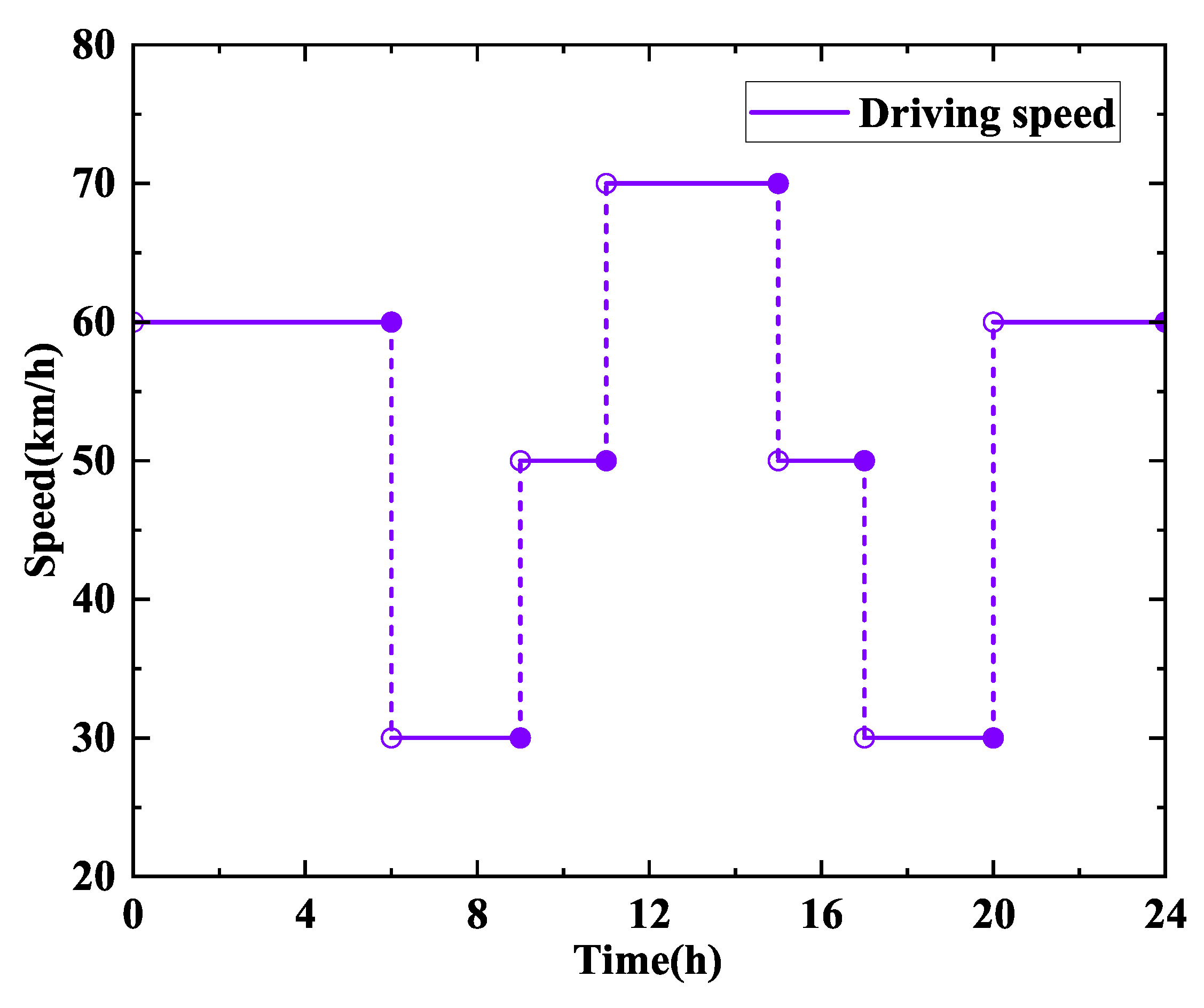
2.3. Time-Varying Speed Function

The time-varying speed model is employed to describe the impact of road traffic conditions on vehicle speeds across different time periods, considering that traffic conditions may vary throughout the day. Vehicle speed is influenced not only by physical road conditions and speed limits but also by traffic flow. To account for varying traffic conditions at different times of the day, we use a segmentation function to model time-varying speeds, as shown in Figure 1.

The velocity of the vehicle at time t is defined as $s_t$, and this velocity function will be adjusted according to traffic conditions in different time periods. Based on research on road speed limits in Chinese cities [18], we set the traffic speed limits for corresponding time periods using the speed limit values of different periods in Zhenjiang as the baseline. The specific model is as follows:

$$s_t=\left\{\begin{array}{cc}60,\hfill & 0<t\le 7\hfill \\ 30,\hfill & 7<t\le 9\hfill \\ 50,\hfill & 9<t\le 11\hfill \\ 40,\hfill & 11<t\le 15\hfill \\ 50,\hfill & 15<t\le 17\hfill \\ 30,\hfill & 17<t\le 20\hfill \\ 60,\hfill & 20<t\le 24\hfill \end{array}\right.$$

(1)

where $s_t$ represents the average speed of vehicles during time period t, measured in km/h. This segmentation function captures the influence of traffic flow on vehicle speed across different time intervals. During the early morning hours, when traffic flow is low, vehicles can maintain a high speed (60 km/h), whereas during peak hours, when traffic congestion increases, vehicle speed decreases to 30 km/h. This trend is particularly pronounced during the evening peak and early morning hours.

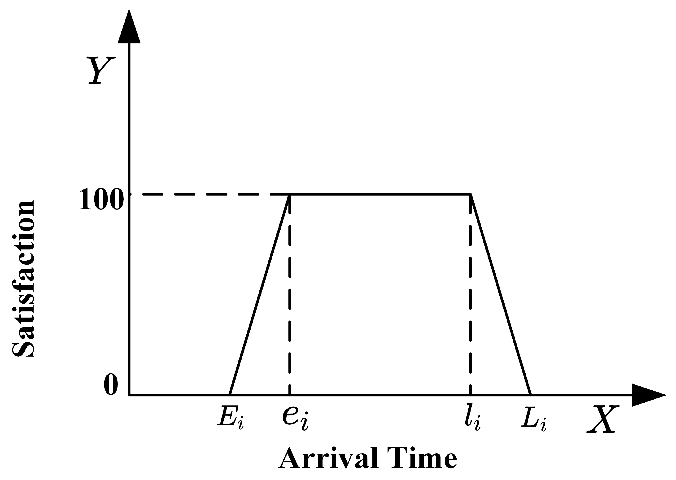
2.4. Customer Satisfaction Trapezoidal Fuzzy Function

Customer Satisfaction Degree (CSD) is a quantitative metric used to assess the disparity in customers’ perceptions of the products and services offered by an organization. Customer satisfaction is influenced by numerous factors, particularly the punctuality, accuracy, and completeness of distribution, which are pivotal in shaping customers’ perceptions of logistics services. Among these, punctuality is directly linked to the expected time window for product delivery.

Due to the dynamic changes in vehicle arrival times during the delivery process, the arrival time may deviate from the customer’s expected time window, which can affect customer satisfaction. Therefore, the model in this study uses a time window function to quantify customer satisfaction.

In traditional hard time window functions, satisfaction is 100 only when the delivery time falls within the customer’s acceptable time range; otherwise, it is 0. We believe that this function is too strict and does not fully reflect the real psychological needs of customers. Therefore, in this study, we use a trapezoidal fuzzy function to evaluate customer satisfaction in order to more accurately reflect the customer’s true feelings [19].

Compared to traditional hard time window functions and triangular fuzzy functions, the trapezoidal fuzzy function expands a single time point into a time window, allowing for some flexibility in the delivery time. As shown in Figure 2, when the product arrives within the customer’s expected time window $[e_i,l_i]$, customer satisfaction is optimal and typically results in the highest service evaluation.

However, the trapezoidal fuzzy function also incorporates the customer’s tolerance for the delivery time. When the arrival time of an item deviates marginally from the desired time window, within the range $[E_i,e_i]$ or $[l_i,L_i]$, customer satisfaction gradually declines as the time deviation increases. This suggests that even if the time deviation remains within a specified range, the customer may still accept it; however, satisfaction diminishes as the deviation increases.

However, when the delivery time exceeds the acceptable time window $[E_i,L_i]$, i.e., when the arrival time of the goods surpasses the maximum range acceptable to the customer, the customer will experience dissatisfaction and may provide a negative evaluation of the delivery service. Therefore, the trapezoidal fuzzy function dynamically incorporates the customer’s tolerance for time window deviation into the satisfaction assessment by adjusting the customer’s desired time window, thereby making the customer’s demand more flexible and accurately reflected in the path planning and delivery service.

2.5. Time Penalty Cost Function

According to the aforementioned model, each customer is assigned a specific delivery time window, which defines the acceptable range of time for the delivery vehicle to arrive. If the delivery vehicle fails to arrive within this window, a financial penalty is incurred, represented by a penalty cost function. The magnitude of the penalty is typically determined by the agreement between the distribution center and the customer and is proportional to the deviation between the actual arrival time of the vehicle and the specified time window. This penalty is designed to encourage timely deliveries, ensuring that the distribution process adheres to customer expectations. The penalty function is expressed as follows:

$$C_t\left(t_i\right)=\left\{\begin{array}{cc}100(1-{\displaystyle \frac{t_i}{e_i}}),\hfill & t_i<e_i\hfill \\ 0,\hfill & e_i<t_i<l_i\hfill \\ 100(1-{\displaystyle \frac{l_i}{t_i}}),\hfill & t_i>l_i\hfill \end{array}\right.$$

(2)

The function can be expressed as:

$$C_t\left(t_i\right)=100\left(1-{\displaystyle \frac{t_i}{e_i}}\right)+100\left(1-{\displaystyle \frac{l_i}{t_i}}\right),t_i\in [E_i,L_i]$$

(3)

where $e_i$ denotes the earliest service time requested by the customer and $l_i$ denotes the latest service time requested by the customer. The range of $[E_i,L_i]$ is set to 10% of $[e_i,l_i]$.

If the vehicle arrives at the customer’s point before time $e_i$ and after $E_i$, it will incur early arrival loss; if the vehicle arrives at the customer’s point after time $l_i$ and before $L_i$, it will incur delayed arrival loss; if the arrival time is beyond the customer’s requested time range $[E_i,L_i]$, the customer will refuse to accept the goods, and then the time penalty cost will tend to be infinity. The penalty function takes into account the impact of time window constraints on service costs and quantifies the negative effects of advancement and delay on customer satisfaction.

2.6. Parameter Definition

To describe the model more accurately, we define the notation used in

Table 1. Symbol description.

Symbol	Symbol Description	Unit
N	Customer Point Assembly	\
K	Distribution Vehicle Collection, denoted by subscript k	\
O	Distribution Center, denoted by subscript o	\
H	Charging Station Collection	\
Z	Collection of distribution centers, customer points, and charging stations, subscripted as z, $Z=N\cup O\cup H$	\
C	Transportation cost per unit placement distance of the distribution vehicle	\
$d_{ij}$	Distance from point i to point j, $i,j\in Z$	m
$q_i$	Demand quantity of the customer at point i, $i\in N$	t
Q	Rated load capacity of the delivery vehicle	t
$t_i^{+}$	Arrival time of the delivery vehicle at point i	\
$t_i^{-}$	Time for the delivery vehicle to leave point i	\
$w_i\left(t\right)$	Time for the delivery vehicle to wait at point i, $i\in Z$	min
$e_i$	Earliest service time requested by the customer at point i, $i\in N$	\
$l_i$	Late service time requested by the customer at point i, $i\in N$	\
$[E_i,L_i]$	Time interval in which the customer can accept the shipment Time interval	\
$t_{ij}$	The time required for the delivery vehicle to travel from point i to point j, $i,j\in Z$	min
$t_i^k$	The time taken by the delivery vehicle k to get to point i, $i\in Z$	\
$p_i^k$	The remaining charge of the delivery vehicle k when it is at point i, $iinZ$	\
P	The battery capacity of the delivery vehicle	\
$s_t$	Speed at which the delivery vehicle is traveling at different times, $t\in [0,24]$	m/s
$x_{ij}^k\in \{0,1\}$	Delivery vehicle k from point i to point j, $k\in K,i,j\in Z$	\
$y_i^k\in \{0,1\}$	Customer i delivery done by vehicle k, $kinK,i,j\in N$	\

:

2.7. Proposed Optimization Formulation

Based on the above assumptions and parameter definitions, we can establish the following mathematical model based on our analysis.

Objective function:

$$\min z=C\sum _{k\in K}\sum _{i\in Z}\sum _{j\in Z,j\ne i}{x}_{ij}^k{d}_{ij}+\sum _{k\in K}\sum _{i\in N}{C}_t\left(t_i\right)$$

(4)

The constraints are:

$$\sum _{i\in N}{y}_i^k{q}_i\le Qk\in K$$

(5)

$$\sum _{i\in N}\sum _{j\in N,j\ne i}{x}_{ij}^k\le \left|N\right|k\in K$$

(6)

$$\sum _{k\in K}\sum _{i\in Z,i\ne o}{x}_{oi}^k\le \left|K\right|$$

(7)

$$p_i^k\ge 0$$

(8)

$$t_i^{-}=0$$

(9)

$$x_{ij}^k,y_i^k\in \{0,1\}i,j\in V,k\in K$$

(10)

$$t_{ij}=d_{ij}/s_{t}i,j\in Z$$

(11)

$$\sum _{k\in K}\sum _{i\in Z}{x}_{oi}^k-\sum _{k\in K}\sum _{j\in Z}{x}_{oj}^k=0$$

(12)

$$\sum _{i\in Z,i\ne j}{x}_{ij}^k=\sum _{j\in Z,i\ne j}{x}_{ij}^k=y_i^{k}k\in K$$

(13)

$$t_j^{+}=\sum _{i\in Z}\sum _{j\in Z,i\ne j}{x}_{ij}^k(t_i^{-}+t_{ij})k\in K$$

(14)

$$w_i\left(t\right)=max[0,(e_i-t_i^{+})]i\in Z$$

(15)

$$p_i^k=Pi\in O\cup H,k\in K$$

(16)

$$t_i^{-}=t_i^{+}+f_i\left(t\right)+w_i\left(t\right)i\in N\cup H$$

(17)

$$C_t\left(t_i\right)=100\left(1-{\displaystyle \frac{t_i}{e_i}}\right)+100\left(1-{\displaystyle \frac{l_i}{t_i}}\right),t_i\in [E_i,L_i]$$

(18)

The objective function is represented by Constraint (4). Constraint (5) ensures that the total amount of goods required by the customers served by each delivery vehicle is less than the rated load capacity of the vehicle. Constraint (6) indicates that the number of customer points served by each vehicle is equal to the total number of customer points. Constraint (7) ensures that the total number of electric vehicles assigned to customer service is less than or equal to the total number of electric vehicles owned by the distribution center. Constraint (8) guarantees that each delivery vehicle has enough battery power to reach the customer points on its planned delivery route, including the distribution center or battery swapping stations. Constraint (9) specifies that the time at which the delivery vehicle leaves the distribution station is zero. Constraint (10) indicates that the decision variables $x_{ij}^k$ and $y_i^k$ are binary variables. Constraint (11) represents the travel time for a delivery vehicle between points i and j, which is calculated as the Euclidean distance between the two points divided by the vehicle’s current travel speed during the time period. Constraint (12) ensures that each delivery task starts and ends at the distribution center. Constraint (13) indicates that each customer point can only be served once. Constraint (14) expresses that the time of arrival at point j for a delivery vehicle equals the time of departure from the previous point i, plus the travel time from point i to point j. Constraint (15) states that if a delivery vehicle arrives at customer point i earlier than the earliest service time $e_i$ for that customer point, the vehicle must wait until $e_i$ before starting the service. The waiting time $w_i\left(t\right)$ is given by $e_i-t_i^{+}$; otherwise, no waiting is required, and $w_i\left(t\right)$ is 0. Constraint (16) specifies that the departure time from customer point i equals the arrival time at point i, the service time at point i, and the waiting time at point i combined. Constraint (17) represents the penalty cost function, while Constraint (18) provides an alternative expression for the penalty cost function.

3. Solution Approach

In this paper, we propose an efficient Genetic Algorithm (GA)-based method that employs a two-population synergistic mechanism consisting of elite and exploratory populations. The specific parameters are $N_{iter}$, $P_{num}$, $P_{mut}$, $Fit$, $M_s$, and $M_{iter}$. The first five parameters represent standard settings in GA, whereas $M_{iter}$ is unique to the two-population approach. The number of iterations $N_{iter}$, the population size $P_{num}$, and the probability of mutation $P_{mut}$ collectively determine the evolutionary direction of the population, while the fitness function $Fit$ governs both the acceptance and stopping criteria of the solution. The stopping condition $M_s$ is based on the “non-improving solution” criterion, whereby the outer loop terminates if the solution does not undergo any change within a specified number of iterations. The migration interval parameter $M_{iter}$ regulates the frequency of communication between the two populations and updates the optimal individuals in each population, thereby preventing redundant computational processes. The specific features of DPCGA will be described in detail in the following sections.

3.1. Algorithm Overview

In real-world vehicle path problems, the constraints are intricate and complex, and the problem scale is relatively large. GAs have been widely applied by experts and scholars in solving vehicle path problems due to their powerful parallel search capabilities, ability to avoid local optima, and advantages such as self-learning, self-organization, and self-adaptation [20]. Many features of the GA are well-suited for solving the electric vehicle-based VRP model examined in this paper; thus, the GA chosen for this study has been specifically designed as the solution method for the problem.

3.1.1. Basic Concepts of Genetic Algorithm

In GA, chromosomes are typically represented by vectors, such as $X=x_1,x_2,\dots ,x_n$, where $x_n$ is a gene, the basic unit of a chromosome. The representation can vary depending on the algorithm, with common forms including binary strings, real-valued strings, and symbolic strings [21]. Binary strings are often used for discrete optimization, while real-valued strings are suited for continuous problems. Choosing the appropriate representation is crucial for algorithm performance, as it affects the efficiency of genetic operations like selection, crossover, and mutation.

Encoding transforms a real-world problem’s solution space into a genotype suitable for the algorithm, ensuring effective exploration of the search space. Once a solution is found, decoding converts the genotype back into a meaningful solution for the original problem. This process is essential for ensuring that the GA provides practical results.

The population in GA consists of individuals, with the population size $P_{num}$ playing a significant role in performance. A small population increases speed but risks premature convergence, while a large population expands the search space at the cost of computational efficiency. Fitness, calculated via a fitness function, measures how close individuals are to the optimal solution and guides the selection process. Genetic operators—selection, crossover, and mutation—drive the algorithm’s evolution, with selection based on fitness, crossover creating offspring from parents, and mutation maintaining diversity to avoid local optima [22,23].

3.1.2. The Characteristics of Genetic Algorithms

GAs have seven significant advantages over other modern heuristic algorithms [24]:

• GAs deal with strings encoding a set of parameters rather than the parameters of a problem, which allows them to be widely used in a variety of fields, including optimization, machine learning, image processing, etc.
• In solving the problem, once the genetic strategy is determined, the GA will use the information in the evolutionary process to organize its own search, and can automatically adapt to the complexity of the problem and optimize the search process.
• GA has the advantage of parallel search, can explore the space of multiple solutions at the same time, so as to effectively deal with the huge amount of data, and adapt to the needs of complex computing.
• GA has strong scalability, can be mixed with other optimization algorithms to expand the scope of application, and make it adaptable in more fields.
• GA does not easily fall into the local optimal solution in the search process, especially in the case of irregular or discontinuous fitness function; it still has a greater possibility to find the global optimal solution.
• GA simulates the evolution mechanism of nature, and can efficiently solve some complex optimization problems, especially multi-peak optimization problems and complex problems with multiple constraints.
• As a kind of heuristic algorithm, GA utilizes probability rules to guide the search direction, does not have special requirements on the search space, and is able to carry out effective search in the discrete complex space, which is especially suitable for large-scale or even super-large-scale complex problems.

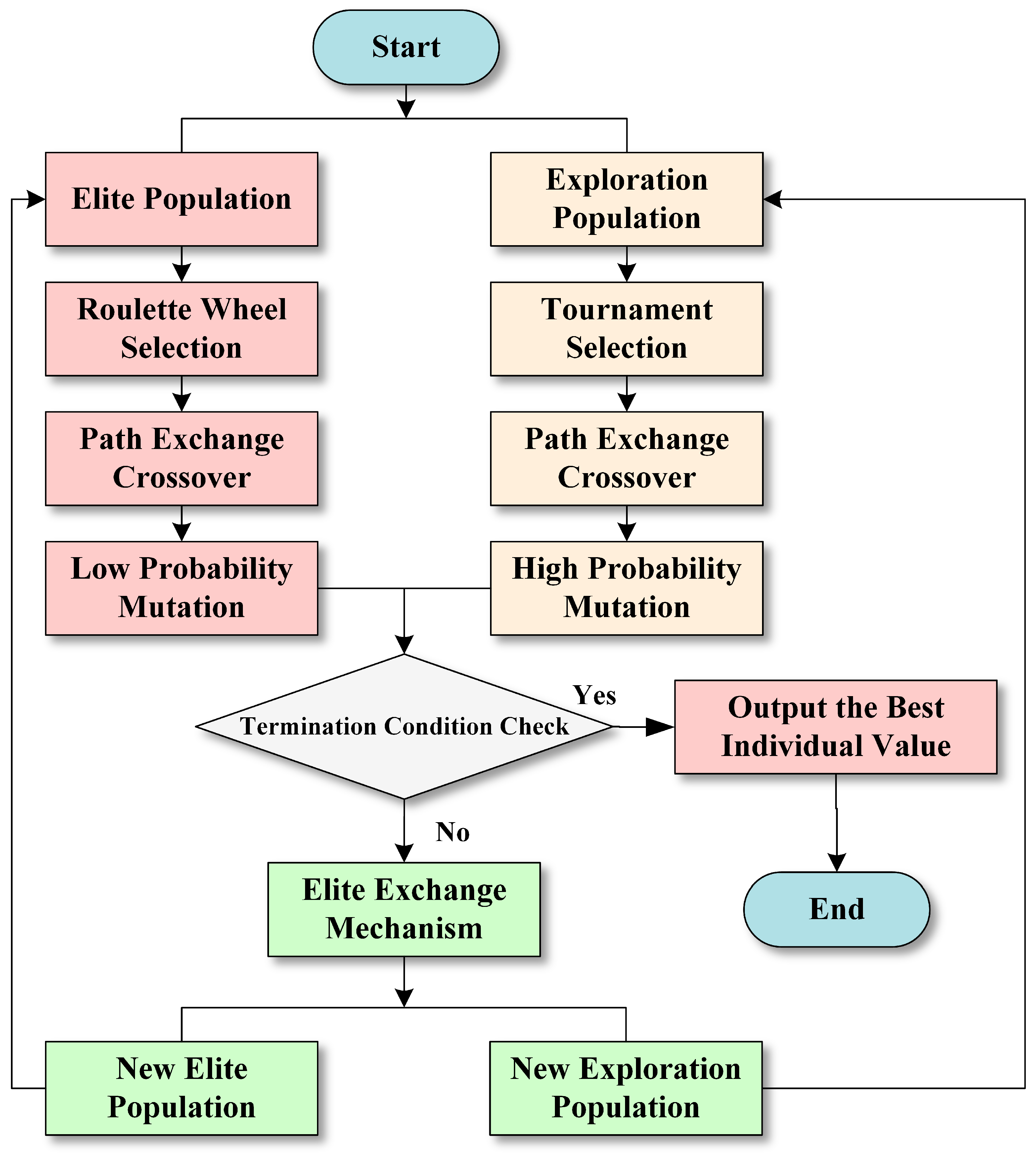
3.2. Algorithm Design

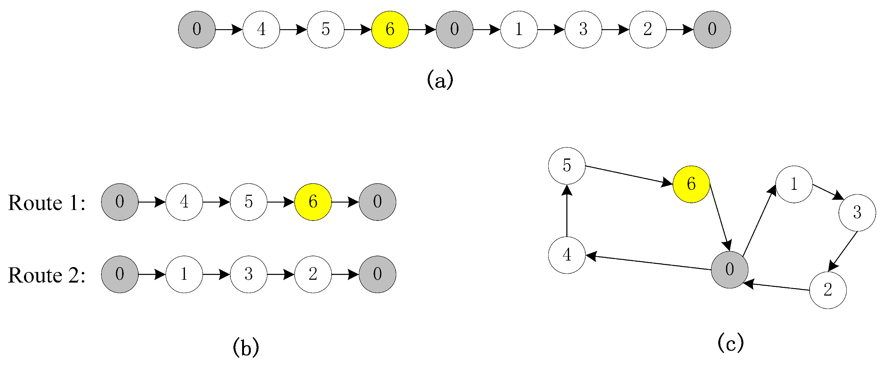
3.2.1. Encoding Scheme Design

Based on the model’s characteristics, this paper employs the natural number coding method with a chromosome length of $m+n+1$, where m represents the number of charging stations and n represents the number of customers. The distribution center is assigned the code 0, while codes 1, 2, 3, …, n represent the fixed codes for each customer, and codes $n+1,n+2,n+3,\dots ,n+m$ correspond to the charging stations.

For example, if the distribution center needs to serve five customers with one charging station available, one chromosome is shown in Figure 3a. In the figure, the gray circle denotes the distribution center, the yellow circle the charging station, and the white circles the customers. After splitting the chromosome, two distinct routes are generated, representing the paths of two carts, as shown in Figure 3b. Route 1 shows the first cart departing from the distribution center, visiting customers 4 and 5, stopping at charging station 6 to recharge, and then returning. Route 2 shows the second cart departing from the center, visiting customers 1, 3, and 2 in sequence, and then returning directly to the distribution center.

Figure 3c shows the actual physical location.

3.2.2. Population Initialization

First, all customer points and charging station numbers are arranged in an array, followed by a randomized perturbation. Let $q_i$ represent the quantity of goods demanded by the ith customer in the chromosome. When ${\sum }_{i=1}^x{q}_i\le Q$ and ${\sum }_{i=1}^{x+1}{q}_i>Q$, a 0 is inserted after the xth position in the chromosome, and the calculation is then performed again from the inserted 0 until position $n-1$. Finally, a 0 is inserted at both the first and last positions of the chromosome to form the initial chromosome. This process is repeated until each of the two populations generates $P_{num}$ chromosomes, forming the initial elite and explorer populations.

3.2.3. Constraint Handling and Fitness Function

This paper employs the penalty function method to handle the constraints. Based on the problem examined in this paper, the driving range and rated load weight limit of the new energy vehicle must be incorporated as penalty functions, yielding the following objective function:

$$\min z=C\sum _{k\in K}\sum _{i\in Z}\sum _{j\in Z,j\ne i}{x}_{ij}^k{d}_{ij}+C_t\left(t_i\right)+M_{1}max\left(\sum _{i\in P_{\mathrm{num}}}{q}_i-Q,0\right)+M_{2}max\left(-p_v^k,0\right)$$

Since these two constraints must be strictly satisfied, $M_1$ and $M_2$ are selected as very large positive numbers, ensuring that when the constraints are violated, the objective function value for this chromosome becomes excessively large. In the objective function, $C_t$ represents the time penalty cost.

The fitness function must be maximized, so we use the inverse of the above objective function as the fitness function, i.e.,

$$\mathrm{fit}\left(i\right)={\displaystyle \frac{1}{z}}$$

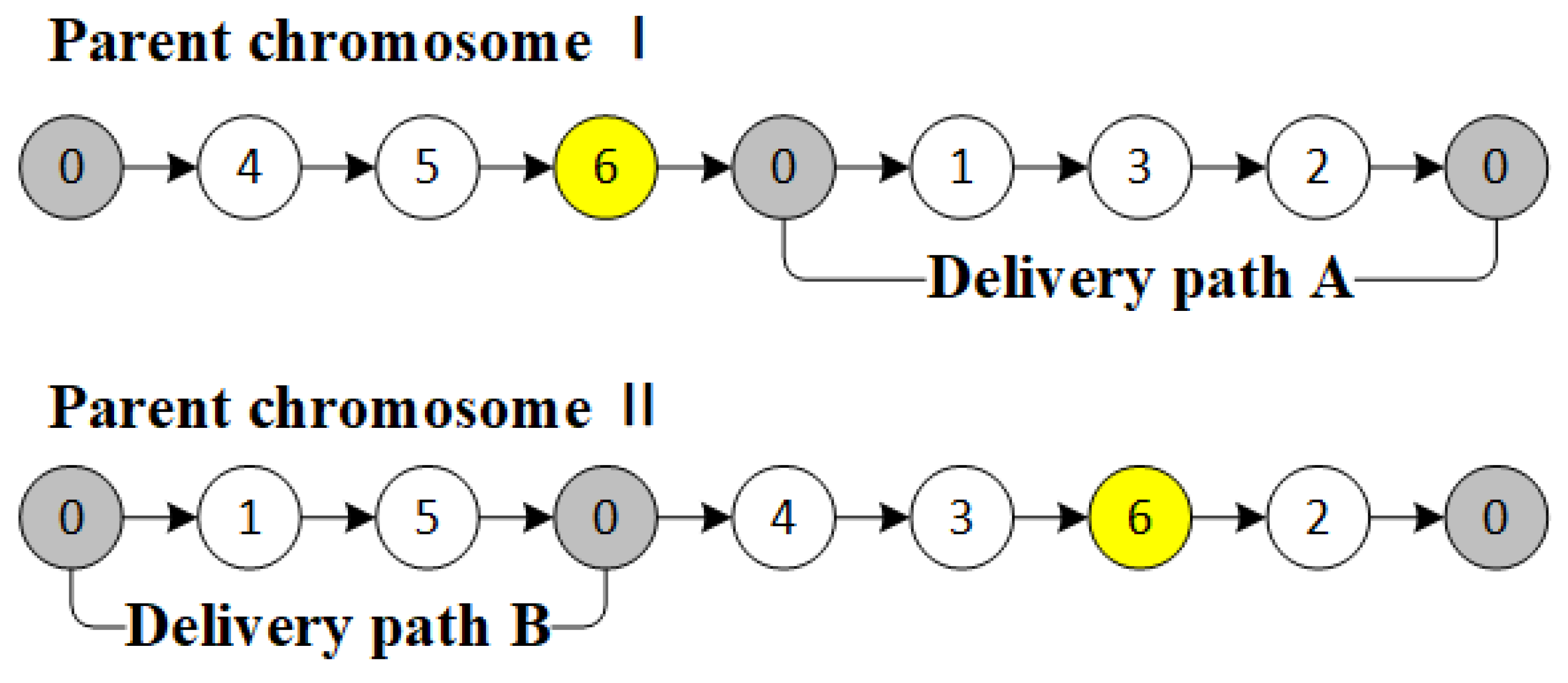
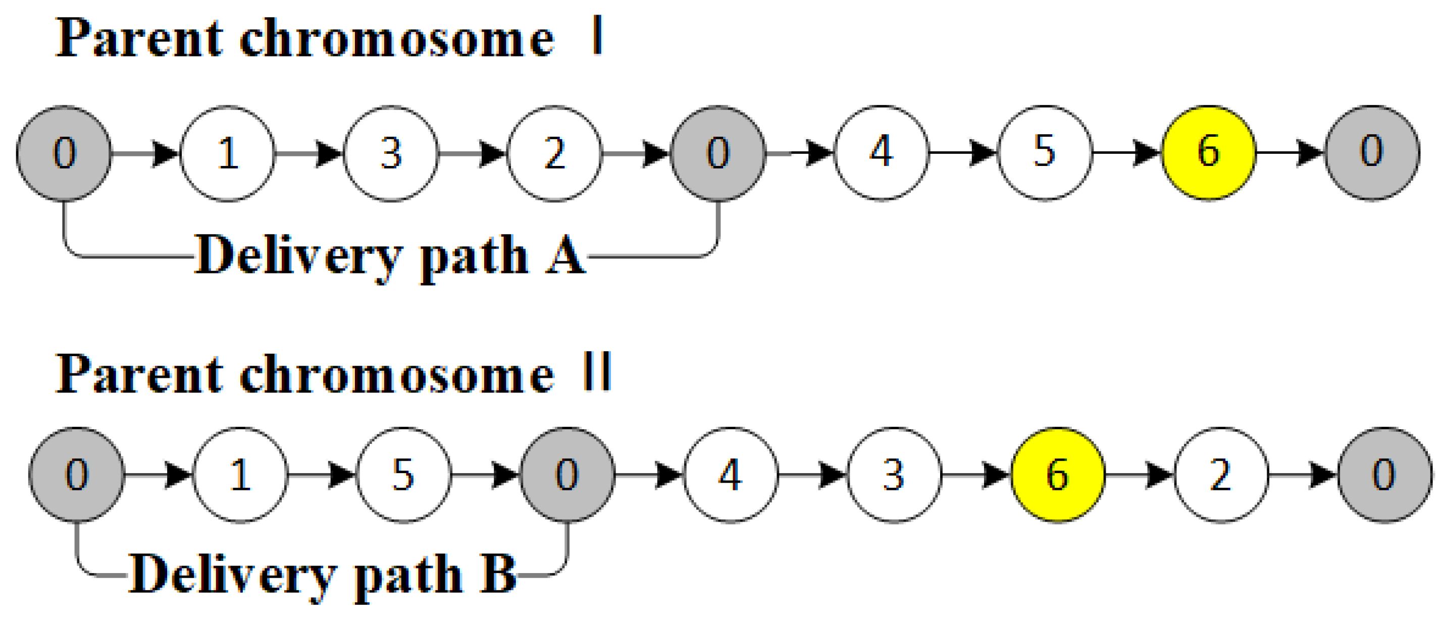
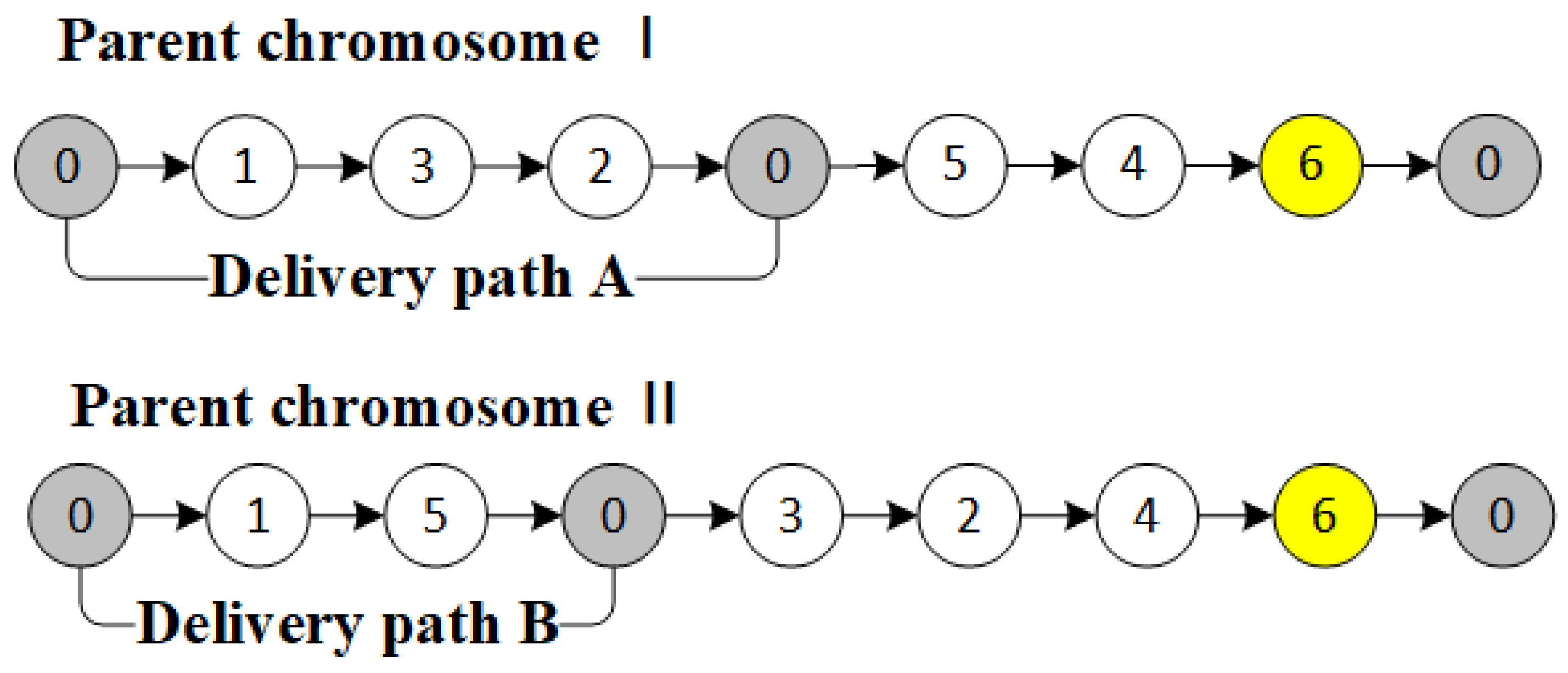
3.2.4. Genetic Operators

(1) Selection and reproduction

In this paper, two algorithms, tournament selection and roulette wheel selection, are applied to the elite population ($P_1$) and the exploratory population ($P_2$) based on their different characteristics. Tournament selection randomly selects individuals for competition, with strong selection pressure, which can accelerate the transfer of superior individuals and performs better when the fitness distribution is uneven. Roulette wheel selection, on the other hand, chooses individuals based on their fitness probabilities. It is simple and intuitive, helps maintain population diversity, is suitable for uniform fitness distributions, and prevents premature convergence to local optima. Both have their advantages; tournament selection is suitable for elite populations, while roulette wheel selection helps explore the diversity of the exploratory population [25,26]. The specific steps are as follows:

For the elite population $P_1$, three individuals are randomly selected from the population, their fitness values $fit\left(i\right)$ are compared, and the individual with the best fitness value is chosen as the parent.

For the exploratory population $P_2$, the fitness $fit\left(i\right)$ of each chromosome is calculated, followed by the calculation of the sum of all fitness values, denoted as $sumfit$. Next, the selection probability $p\left(i\right)$ for each chromosome is computed, and the cumulative probability $pc\left(i\right)$ is subsequently determined.

A random number r in the interval $[0,1]$ is then generated. If $pc\left(i\right)>r$, the ith chromosome is selected; otherwise, the ith chromosome that satisfies $pc(i-1)<r\le pc\left(i\right)$ is selected.

The detailed algorithm is provided in Algorithm 1.

Algorithm 1: Roulette and Tournament

(2) Crossover

Many natural number-encoded crossover methods, such as sequential and cyclic crossover, are commonly used to solve TSP problems, but tend to perform poorly in vehicle path optimization problems involving multiple delivery vehicles and subpaths. To enhance the algorithm’s ability to find optimal solutions in the later evolutionary stages, this paper proposes an improved crossover operator designed to maximize the retention of high-quality sub-path information from the parent generation. The steps are outlined as follows:

Step 1: Randomly select a vehicle’s distribution path among the two parent chromosomes, such as Figure 4:

Step 2: Fronts the selected distribution path (Figure 5):

Step 3: The distribution path A in parent chromosome 1 is used as part of daughter chromosome 1. Simultaneously, the missing code in distribution path A from parent chromosome 2 is added to the end of distribution path A in daughter chromosome 1, following the order in parent chromosome 2, and a complementary code of 0 is added at the end of the chromosome. A similar operation is applied to daughter chromosome 2 (Figure 6).

(3) Mutation

The three-point exchange mutation operator was employed to mutate the parent chromosomes [27], wherein three positions were randomly selected from the parent chromosomes for exchange, resulting in five offspring chromosomes. The fitness of each offspring was then calculated, and the individual with the highest fitness was added to the offspring population.

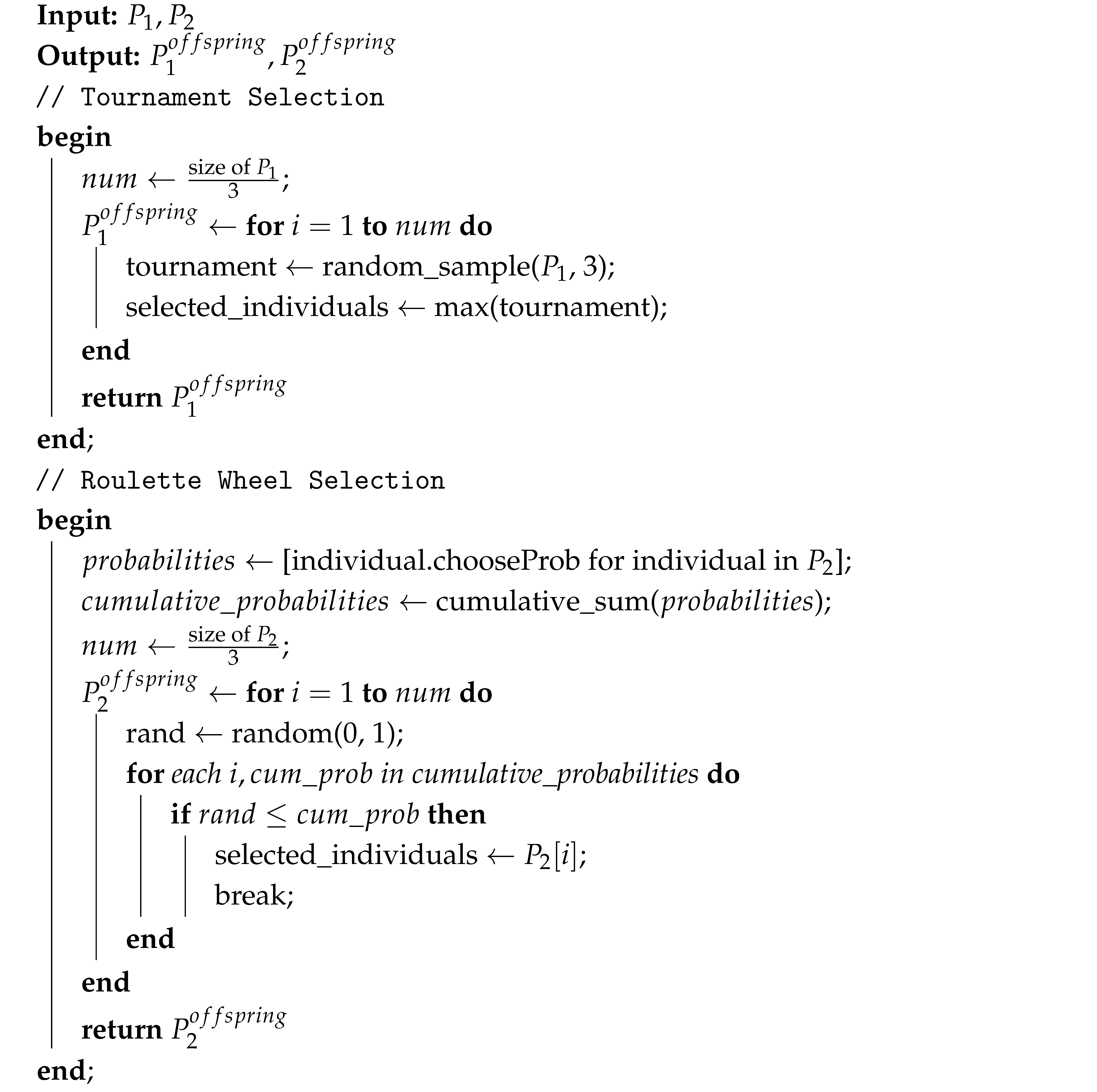3.2.5. Termination Condition

The GA is a stochastic search method, and to terminate its evolutionary process, termination conditions must be pre-set. Three common termination conditions are typically used: first, achieving a predetermined goal; second, when the optimal individual in the population does not improve over a specified number of consecutive generations; and third, reaching a predetermined maximum number of evolutionary generations. By setting the condition of “no further improvement in the optimal individual over a specified number of generations”, the algorithm can be terminated at an appropriate time to avoid over-computation. Therefore, in this paper, we select the termination condition of “no progress over several generations”.

3.2.6. Dual-Population Collaborative Mechanism

In the two-population synergistic mechanism, every 10 generations, the top 10% of the best individuals from the elite and exploratory populations are exchanged to facilitate information exchange and optimization. Simultaneously, the mechanism discards the worst 10% of individuals from each population to maintain diversity and prevent excessive convergence.

3.3. Dual-Population Collaborative Genetic Algorithm (DPCGA)

Figure 7 illustrates the detailed flow of the algorithm. After initializing the elite population ($P_1$) and the exploratory population ($P_2$), offspring are selected using tournament selection and roulette wheel selection, respectively. The selected offspring undergo crossover and mutation operations and are subsequently integrated into the original population. The algorithm terminates the loop when the fitness values of the optimal individuals in consecutive $M_s$ generations do not change; otherwise, the algorithm continues the coordination mechanism of the two populations, where the top 10% of the best individuals from each population are exchanged, and the bottom 10% are discarded every $M_{iter}$ generations to maintain population size stability. This ensures fast and stable convergence.

Algorithm 2 outlines the DPCGA algorithm, where $N_{iter}$ represents the number of iterations, $P_{num}$ denotes the number of chromosomes in the population, and $M_{iter}$ refers to the number of generations between exchanges of the two populations. $M_s$ is the number of consecutive iterations without improvement in the solution. This parameter indicates the number of iterations during which no better solution is found. The algorithm proceeds as described.

Algorithm 2: DPCGA

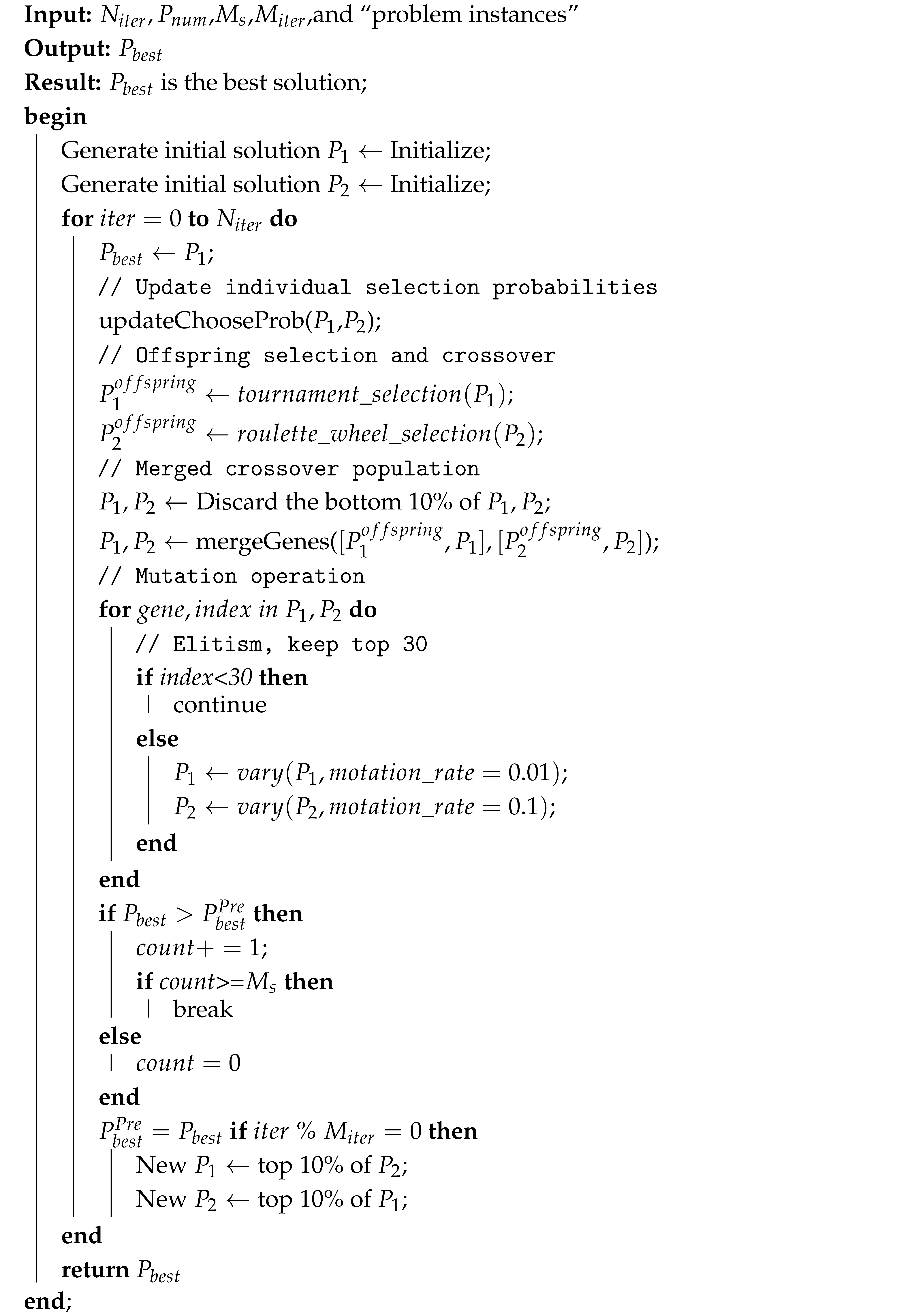4. Experiment

To verify the optimization capability and stability of the DPCGA algorithm, two experiments were designed in this paper. The first experiment compares the DPCGA algorithm with the representative VRP problem-solving algorithm VRPTW proposed in the literature in this field to assess its performance in solving similar problems. The second experiment is conducted on a more challenging dataset generated by a computer, aiming to examine the solving effect of the DPCGA algorithm in complex problems and systematically compare it with the ESA-VRPO and AVNS algorithms. Both experiments were implemented in Python 12.7 and run on a computer equipped with a 12th Gen Intel(R) Core i7-12700H (2.3 GHz), RTX 3060 Laptop GPU, and Windows 12 as the operating system. Through these two experiments, we comprehensively evaluate the optimization capability and stability of the DPCGA algorithm under different problem scales and complexities, thereby providing more sufficient theoretical support for its performance in practical applications.

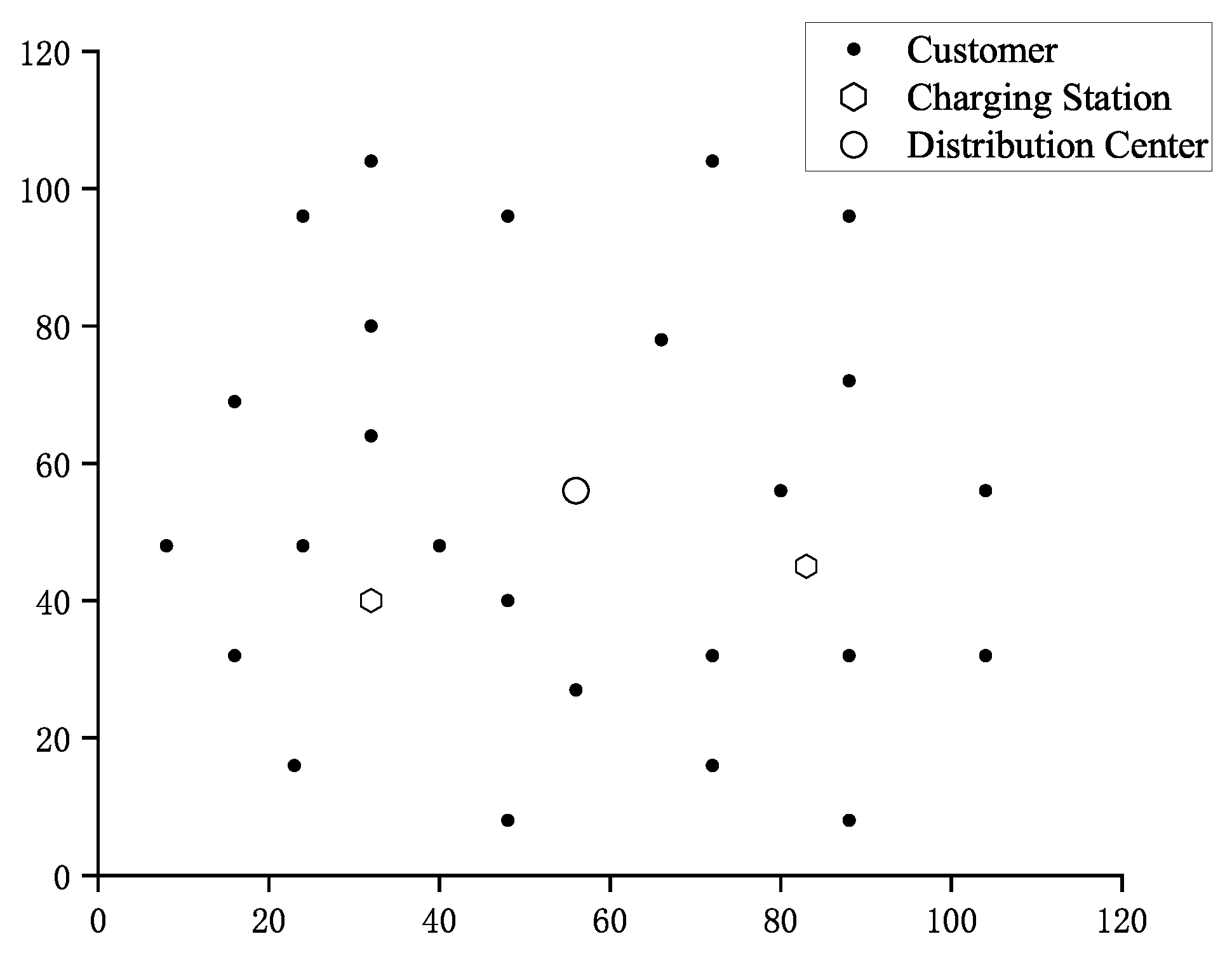
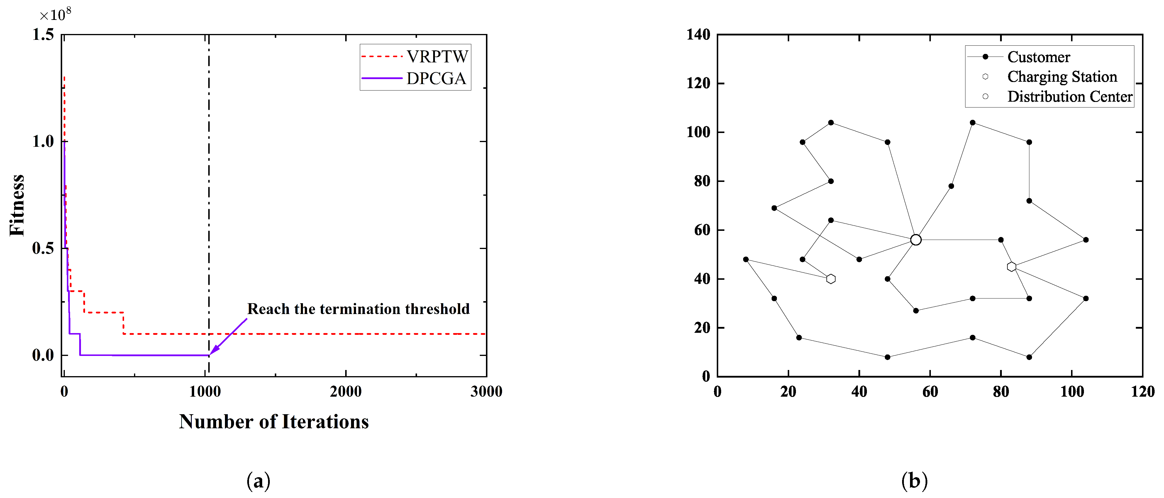
4.1. Test Instances-1

The dataset used in this experiment, serving as a benchmark for the comparative study, is derived from the work of Gao et al. [28] For details on the dataset’s generation process and background, readers are referred to their original paper. This dataset includes 25 customer locations and two charging stations, with the distribution center located at [56,56]. By using this standard dataset, we can conduct a fair and systematic performance evaluation of our algorithm, effectively comparing it with other existing research results to validate the strength and applicability of our approach.

Figure 8 shows the specific location distribution of distribution centers, charging stations, and customer points for this dataset.

4.1.1. Environment and Parameter Settings

In the comparison with the VRPTW algorithm [28], the original Matlab 2014a code was converted into a Python-compatible version to allow for a comparison of its performance with our proposed algorithm. In the experiments, the $N_{iter}$ parameter is set to 3000, and the $P_{num}$ parameter is set to 100. In addition, in our DPCGA algorithm, $M_s$ is introduced as a threshold for stopping iteration, set to 200, to further enhance efficiency and convergence. A population exchange mechanism is also incorporated, where an exchange of information occurs every $M_{iter}$ generations. This ensures the comparability and fairness of the algorithms, providing robust data support for analyzing their performance under specific conditions.

4.1.2. Experimental Results

Figure 9a shows the comparison between the DPCGA algorithm and the VRPTW algorithm in terms of convergence speed. As shown in the figure, the DPCGA algorithm converges significantly faster than the VRPTW. The fitness value of the DPCGA decreases rapidly and stabilizes around 1000 iterations, while the VRPTW shows a slower rate of decrease and fails to converge quickly before 2000 iterations. This comparison suggests that DPCGA reaches the optimal solution more efficiently in fewer iterations. Additionally, the dashed vertical line in the figure marks the point at which the DPCGA algorithm reaches the termination threshold and ends the run, further highlighting the efficiency of DPCGA.

Figure 9b shows the corresponding distribution path.

Table 2. Detailed algorithm data comparison.

Algorithm	NoV	RT (s)	DC
DPCGA	3	11	6494.9
VRPTW	3	24	6542.7

NoV: number of vehicles. RT: convergence time. DC: delivery cost.

presents the comparison of the two algorithms, DPCGA and VRPTW, based on key performance metrics. The data in the table clearly indicate that the DPCGA algorithm significantly outperforms VRPTW in runtime (RT) with the same number of vehicles (NoV = 3), showing an optimization of approximately 54%. Additionally, DPCGA also demonstrates some optimization in distribution cost (DC), which is reduced by approximately 1.5% compared to VRPTW. This demonstrates that the DPCGA algorithm outperforms the VRPTW algorithm in both optimization capability and runtime for this type of problem.

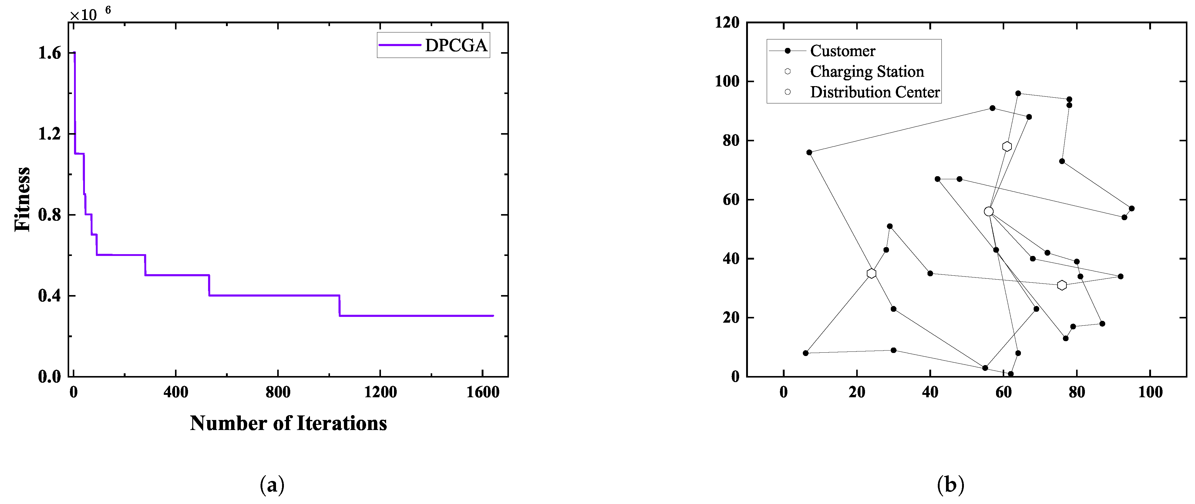
4.2. Test Instances-2

In Example 2, we simulated scenarios at different scales. Since there is currently no standard test set for vehicle routes with charging station coordinates, this study uses Solomon’s test set as the benchmark, on which a dataset (

Table A1. Test Instances-2 dataset.

Index	X	Y	T	en	lh	Server
0	56	56	0	0	100	0
1	64	96	0.28	7	21	0.3
2	80	39	0.12	12	16	0.4
3	69	23	0.47	6	11	0.1
4	72	42	0.16	5	11	0.1
5	48	67	0.06	6	14	0.3
6	58	43	0.12	10	20	0.4
7	81	34	0.36	5	11	0.4
8	79	17	0.45	9	17	0.2
9	30	23	0.34	7	13	0.4
10	42	67	0.03	11	19	0.4
11	7	76	0.22	5	20	0.3
12	29	51	0.47	4	19	0.3
13	78	92	0.08	10	22	0.1
14	64	8	0.36	11	20	0.4
15	95	57	0.31	4	16	0.2
16	57	91	0.29	6	6	0.4
17	40	35	0.05	12	20	0.2
18	68	40	0.35	5	12	0.1
19	92	34	0.42	3	7	0.1
20	62	1	0.24	2	9	0.2
21	28	43	0.13	9	14	0.2
22	76	73	0.07	2	12	0.1
23	67	88	0.24	12	17	0.1
24	93	54	0.12	4	13	0.2
25	6	8	0.39	10	13	0.4
26	87	18	0.05	7	16	0.3
27	30	9	0.08	7	14	0.2
28	24	35	0	0	100	0.4
29	61	78	0	0	100	0.4
30	76	31	0	0	100	0.4

) with a random number of charging stations matching the customer points is generated. The specific details are shown in

Table 3. Parameters of instances.

Scale	${\mathit{N}}_{\mathit{p}}$	${\mathit{N}}_{\mathit{s}}$	$\mathbf{MNSV}$
Small	30	3	4
Medium	50	5	5
Large	100	8	7

$N_p$: number of customer points. $N_s$: number of charging stations. MNSV: maximum number of vehicles.

. We selected five different datasets for each type, such as C101 to C105 for 100 customer points of Type C. To evaluate the algorithm’s performance, we conducted 20 independent runs for each dataset and calculated the average, standard deviation, and average runtime of these 20 runs. At the same time, the comparison between the algorithm and the benchmark model followed the same process.

The parameters of the distribution vehicle are based on publicly available new energy vehicle data and scaled to fit different regional scenarios. The distribution vehicle has a load capacity of 2.5 tons (excluding its own weight) and a maximum range of 310 km. In running the DPCGA algorithm, $N_{iter}$ is set to 3000, $P_{num}$ is set to 100, $M_s$ is set to 200, and $M_{iter}$ is set to 10.

4.2.1. Experimental Results

In this section, we elaborate on the solution process of the DPCGA algorithm and demonstrate the optimal solution using example s_1. Figure 10a shows the convergence trend of the DPCGA algorithm. The fitness value in the figure represents the optimal solution for the elite population at each iteration. As shown in the figure, the algorithm exhibits a faster decreasing trend in the early stages, primarily due to the assistance of the exploratory population, which enables the algorithm to explore better solutions with a higher probability, helping it avoid local optima. After approximately 1000 iterations, the algorithm enters a stable phase, where no new optimal solution is found for 200 consecutive generations, and eventually, the algorithm stops and obtains the optimal solution. Figure 10b shows the complete distribution route for the entire region.

Figure 11 illustrates the optimal distribution routes found by the DPCGA algorithm, along with the number of distribution trolleys used. In Figure 11, the three routes together form the complete distribution scheme, corresponding to the distribution tasks of vehicles $k_1$, $k_2$, and $k_3$, respectively. The gray circles represent the distribution centers, i.e., the starting and ending points of the distribution vehicles, while the yellow circles represent the charging stations. Under this optimal distribution strategy, the average cost per road section is 1217.91. The solution shows that, due to range constraints, the $k_1$ vehicle is charged twice during the distribution process, while $k_2$ and $k_3$ are charged zero times and once, respectively. This indicates that $k_1$ is primarily responsible for long-distance delivery, while $k_2$ and $k_3$ handle short-distance or multi-customer point deliveries.

4.2.2. Algorithm Comparison

To explore the performance of the algorithms, we generated five datasets for different scenarios using the above method and conducted batch experiments. For each dataset, the results obtained using the algorithm proposed in this paper were compared with those from other algorithms. The algorithms compared include the ESA-VRPO algorithm and the AVNS algorithm. The ESA-VRPO algorithm evaluates the difference between the current solution and the new solution by performing a neighborhood search in each iteration, accepting the new solution based on a certain probability. The AVNS algorithm is designed to dynamically adjust performance through a two-stage learning and optimization process, combined with a large-scale neighborhood search (LNS) strategy, to adjust local search operators in response to dynamic events such as traffic and optimize the path.

Table 4. The comparative results of the three algorithms in three different scenarios.

Scale	Name	DPCGA			ESA-VRPO			AVNS
		Avg.DC	NoV	RT	Avg.DC	NoV	RT	Avg.DC	NoV	RT
Small	S1	93.21	3	34	92.98	3	42	92.19	3	45
	S2	91.21	3	33	91.09	3	41	92.01	3	46
	S3	92.23	3	33	91.44	3	46	90.21	3	45
	S4	95.94	3	35	93.22	3	44	94.24	3	46
	S5	94.23	3	31	94.11	3	43	93.13	3	46
Medium	M1	90.25	4	89	89.25	4	94	90.22	4	87
	M2	91.65	4	79	92.15	4	91	91.65	4	91
	M3	94.12	4	80	90.24	4	93	91.02	4	81
	M4	91.28	4	86	90.18	4	100	89.21	4	80
	M5	93.23	4	84	93.03	4	96	91.23	4	91
Large	L1	92.33	6	203	91.23	7	252	89.11	6	289
	L2	91.23	6	254	89.56	6	280	88.98	6	264
	L3	93.45	6	198	90.22	6	232	90.92	7	231
	L4	96.21	7	234	92.32	7	250	90.11	7	255
	L5	92.92	6	267	90.01	6	279	88.21	7	295

Avg.DC: average customer satisfaction. NoV: average number of vehicles. RT: average convergence time.

presents the experimental results of four algorithms across 15 instances in scenarios of varying sizes. Each algorithm is run independently 20 times for each instance in every scenario, with the results presented as averages. The first column of the table lists the scale of the three scenarios, the second column identifies the name of each instance, and the third through fifth columns display the average values of customer satisfaction, the use of delivery vehicles, and the running time of the algorithms, respectively.

In the small-scale scenario, the algorithm proposed in this paper improves customer satisfaction over the ESA-VRPO algorithm by 0.13% to 2.92% and reduces the average runtime by 23.04%. In the other two scale scenarios, performance improvement is similarly significant. In the medium-scale scenario, customer satisfaction improves by 1.12% to 5.07% and the runtime is reduced by 11.8%, while in the large-scale scenario, customer satisfaction improves by 3.44% to 5.06% and the runtime is reduced by 10.82%. Overall, customer satisfaction improves by an average of about 2% across the three scenarios, while runtime is reduced by about 15%. These results demonstrate that the proposed algorithm has a significant advantage over the ESA-VRPO algorithm in terms of customer satisfaction. The main reason for this is that the proposed algorithm optimizes the elite population using the auxiliary population, enabling faster convergence and making it easier to find high-quality solutions, especially in complex environmental scenarios, where it performs better.

The proposed algorithm demonstrates significant performance improvement over the AVNS algorithm. In small-scale instances, the DPCGA algorithm improves customer satisfaction by 1.11% to 2.24% over the AVNS algorithm; in medium-scale scenarios, customer satisfaction improves by 2.64% to 5.67%; and in large-scale scenarios, the improvement ranges from 2.17% to 6.77%. In terms of runtime, the DPCGA algorithm saves 14.25% compared to the AVNS algorithm. These results demonstrate that the DPCGA algorithm proposed in this paper significantly outperforms the AVNS algorithm in all aspects, exhibiting substantial performance improvements.

On the other hand, although the proposed algorithm does not show a significant difference from the other two algorithms in terms of the number of delivery vehicles used, there is only a one-vehicle difference in the mass delivery scenario. This may be due to the fact that in this scenario, the vehicles have sufficient load capacity, resulting in less impact on the total mass of the final distribution goods.

Analyzing the running times of the three algorithms in instances of different sizes, it can be seen that although the AVNS algorithm’s running time is lower than that of the proposed algorithm in some of the instances, this time advantage is only 2.3% to 7.5% in the medium- and large-scale scenarios. However, in general, the computational speed disadvantage of the AVNS algorithm over the proposed algorithm becomes more and more obvious as the problem size increases. For individual shorter time gaps, this disadvantage is acceptable. For the ESA-VRPO algorithm, the running time is significantly longer than the DPCGA algorithm. This runtime disadvantage is more significant in small- and medium-scale instances. However, in large-scale instances, the DPCGA algorithm is still about 10% faster than the other algorithms, even though the gap between the two runtimes has narrowed. In real-world distribution, this time difference still provides significant cost savings.

Table 5. Statistical analysis of algorithm execution times across different scales.

Scale	Algorithm	C	Mean RT	Std Dev RT	95% CI Lower	95% CI Upper
Small	DPCGA	6492.1	33.2	1.48324	31.35831	35.04169
	ESA-VRPO	6572.3	43.2	1.923538	40.81161	45.58839
	AVNS	6511.4	45.6	4.037326	40.587	50.613
Medium	DPCGA	9021.4	83.6	4.159327	78.43551	88.76449
	ESA-VRPO	9194.9	94.8	4.91935	88.69182	100.9082
	AVNS	9188.6	86	5.291503	79.42973	92.57027
Large	DPCGA	13,213.4	231.2	18.8865	207.7493	254.6507
	ESA-VRPO	13,910.8	258.6	20.61068	233.0085	284.1915
	AVNS	14,001.2	266.8	26.06147	234.4404	299.1596

C: Average delivery cost. Mean RT: Average convergence time. Std Dev RT: Standard deviation of convergence time.

presents the statistical analysis of algorithm running times at different scales. As the problem scale increases, the running time (RT) of the algorithms generally increases, and their volatility varies.

At the small scale, the DPCGA algorithm has the shortest running time, with an average of 33.2 s and a standard deviation of 1.48, indicating good computational stability. Its 95% confidence interval ranges from 31.36 to 35.04 s, demonstrating predictable running times. In contrast, the ESA-VRPO algorithm has an average running time of 43.2 s, a standard deviation of 1.92, with a 95% confidence interval of 40.81 to 45.59 s, showing slightly longer and more fluctuating computation times. The AVNS algorithm has the longest running time, with an average of 45.6 s and a standard deviation of 4.04. Its 95% confidence interval ranges from 40.59 to 50.61 s, exhibiting higher volatility.

At the medium scale, the DPCGA algorithm has an average running time of 83.6 s, with a standard deviation of 4.16 and a 95% confidence interval ranging from 78.44 to 88.76 s, showing good stability. The ESA-VRPO algorithm has an average running time of 94.8 s, a standard deviation of 4.92, and a 95% confidence interval from 88.69 to 100.91 s, indicating an increase in computation time and greater fluctuations. The AVNS algorithm has an average running time of 86 s, a standard deviation of 5.29, and a 95% confidence interval from 79.43 to 92.57 s, demonstrating similar volatility to ESA-VRPO.

For the large scale, the running times of all algorithms increase significantly. The DPCGA algorithm has an average running time of 231.2 s, a standard deviation of 18.89, and a 95% confidence interval from 207.75 to 254.65 s, showing larger fluctuations. The ESA-VRPO algorithm has an average running time of 258.6 s, a standard deviation of 20.61, and a 95% confidence interval from 233.01 to 284.19 s, indicating longer computation times and more substantial volatility. The AVNS algorithm has a running time of 266.8 s, a standard deviation of 26.06, and a 95% confidence interval from 234.44 to 299.16 s, showing higher computation times and even greater volatility.

In terms of average delivery costs, at the small scale, the DPCGA algorithm has an average delivery cost of 6492.1, while the ESA-VRPO algorithm’s average is 6572.3, and the AVNS algorithm’s average is 6511.4, indicating that DPCGA has a certain advantage in cost control. As the problem scale increases, at the medium scale, DPCGA’s average delivery cost is 9021.4, and at the large scale, it is 13,213.4. In comparison, the average delivery costs of ESA-VRPO and AVNS also increase. Despite the increase in computation time, the DPCGA algorithm still demonstrates significant advantages in cost control and stability, particularly at the large scale, where, although the average delivery cost significantly increases, DPCGA maintains relatively lower running times and higher stability.

Overall, the DPCGA algorithm exhibits relatively short running times and good stability across all scales, performing exceptionally well at the small and medium scales, demonstrating its efficiency and stability in different computational environments.

5. Sensitivity Analysis

For the DPCGA algorithm, we conducted a sensitivity analysis on two key factors: the number of charging stations and vehicle range, within a medium-scale scenario. In this analysis, we adjusted the number of charging stations (5, 7, and 10) and vehicle range (200 km, 300 km, and 400 km), evaluating their effects on the path planning results through several simulation experiments. We observed the effects of changes in the number of charging stations and vehicle range on customer satisfaction and path planning costs. Through this sensitivity analysis, we aimed to reveal how charging infrastructure and vehicle performance influence the adaptability and optimization of the DPCGA algorithm under varying distribution demands and traffic conditions, providing valuable insights for future algorithmic improvements and practical applications.

5.1. Impact of the Number of Charging Stations on Path Planning Results

Analysis of the data in

Table 6. Impact of different number of charging stations on customer satisfaction and path costs.

	SC-1	SC-2	SC-3	SC-4	SC-5	Average
5	2118.791	2048.583	1840.131	2074.797	1838.124	1984.085
	89.69232	91.144	88.43677	91.38577	91.80182	90.49213
7	2010.093	1767.228	2014.394	1998.466	1926.308	1943.297
	91.67233	89.9857	91.70737	90.36707	90.18211	90.78292
10	2069.498	2019.218	1940.303	1921.587	1843.94	1958.909
	89.37592	88.36692	90.50012	91.97084	92.33602	90.50996

SC: Different data sets. Different Number of Charging Stations first behavior road cost, second behavior customer satisfaction.

indicates that changes in the number of charging stations had little impact on customer satisfaction or path planning costs. Although some fluctuations in path planning costs and customer satisfaction occurred as the number of charging stations increased from 5 to 7 to 10, the overall differences remained minimal.

With five charging stations, the average cost was 1984.09 and satisfaction was 90.49; with seven charging stations, the cost decreased slightly to 1943.30, and satisfaction increased to 90.78; and with ten charging stations, the cost decreased slightly again to 1958.91, and customer satisfaction increased marginally to 90.51. These changes suggest that increasing the number of charging stations within a certain range has a limited effect on path planning optimization, particularly when the changes in cost and customer satisfaction are minimal.

Overall, when the number of charging stations is adequate for the entire distribution process, further increasing their number does not significantly improve route planning costs or enhance customer satisfaction.

5.2. Impact of Vehicle Range on Path Planning Results

From

Table 7. Impact of different range on customer satisfaction and path costs.

	SC-1	SC-2	SC-3	SC-4	SC-5	Average
400 KM	2052.811	2057.504	1967.373	1936.823	2023.002	2007.503
	93.18418	91.08811	91.40597	89.80545	90.03924	91.10459
300 KM	1929.917	1828.329	2366.078	1805.997	2003.629	1986.79
	88.3889	91.63132	92.63935	87.74532	91.67916	90.41681
200 KM	2004.126	2030.209	1996.23	2062.861	2259.379	2070.561
	89.61487	91.58579	88.37952	88.45071	91.35766	89.87771

SC: different datasets. Different ranges: first behavior road cost, second behavior customer satisfaction.

, it is evident that the vehicle’s range significantly impacts both the cost and customer satisfaction of path planning. For vehicles with a 400 km range, the overall cost is higher, but customer satisfaction is also better, with an average satisfaction of 91.1 and an average cost of 2007.50. Vehicles with a longer range can reduce the frequency and duration of charging stops during the journey, thereby simplifying path planning and improving delivery efficiency. This allows vehicles with a 400 km range to complete delivery tasks more quickly while maintaining high customer satisfaction.

In contrast, the 300 km range vehicles exhibit some fluctuations in path planning costs. Although in certain scenarios (e.g., scenarios 2 and 5), the costs were lower, the overall costs remained higher than those of the 400 km vehicles, with an average cost of 1986.79. Despite the increase in customer satisfaction (90.42), the 300 km range vehicles led to higher time consumption and reduced efficiency in path planning due to frequent charging needs.

For vehicles with a 200 km range, the cost is higher, with an average cost of 2070.56, and customer satisfaction is relatively low, with an average satisfaction of 89.88. This suggests that vehicles with a lower range require more charging stations and additional time to complete deliveries, leading to more complex path planning and a greater impact on both cost and customer satisfaction. Therefore, increasing vehicle range can help optimize path planning, reduce costs, and improve overall customer satisfaction.

6. Summary and Conclusions

This study investigates the vehicle routing problem considering time windows, time-varying speeds, and customer satisfaction (VRP-TWTVS-CS), incorporating the selection of charging stations for electric vehicles. A DPCGA algorithm was developed to solve the resulting single-objective optimization. Several key findings were derived from the experiments:

• When using the same dataset as the VRPTW algorithm, the proposed DPCGA algorithm demonstrates excellent performance, finding better solutions with faster convergence times under the same conditions.
• By adopting an evaluation method based on customer satisfaction, the customer satisfaction in VRP-TWTVS-CS improved by an average of 3%, with a 15% reduction in convergence time, and better solutions were found in more complex scenarios. This indicates that in real-world environments, service quality and customer satisfaction can be effectively improved.
• The introduction of the charging station feature further enhances customer satisfaction and alleviates the time waste caused by charging for electric vehicles.

These findings prove the effectiveness of VRP-TWTVS-CS in achieving a balance between cost planning and customer satisfaction.

This paper presents a mathematical model for path planning that considers time windows, time-varying speeds, and customer satisfaction. Due to the complexity of the problem, a DPCGA algorithm is designed, which introduces a dual-population collaborative development mechanism and uses a population selected by roulette wheel selection to assist in the development of the population selected by tournament selection, significantly improving computational efficiency and optimization results. Numerical experiments were conducted to verify the efficiency and effectiveness of the DPCGA algorithm, and the impact of the number of charging stations and vehicle range on customer satisfaction was analyzed.

Although this study has achieved some preliminary results, there are still some shortcomings due to the limitations of the research level that need to be addressed. Future research will focus on further optimizing algorithm performance, especially in efficiently and flexibly delivering goods under dynamic user demand. By quantifying the costs involved in the delivery process and considering real-time user needs, the overall system efficiency can be effectively improved. Furthermore, considering the balance between cost consumption and customer satisfaction, how to precisely control resource consumption during the delivery process will be an important future research task.

References

- Rupnik, B.; Wang, Y.; Kramberger, T. Hybrid Model for Motorway EV Fast-Charging Demand Analysis Based on Traffic Volume. Systems 2025, 13, 272. [Google Scholar] [CrossRef]
- El Wafi, M.; Youssefi, M.A.; Dakir, R.; Bakir, M. Intelligent Robot in Unknown Environments: Walk Path Using Q-Learning and Deep Q-Learning. Automation 2025, 6, 12. [Google Scholar] [CrossRef]
- Han, Z.; Guo, W. Dynamic UAV Task Allocation and Path Planning with Energy Management Using Adaptive PSO in Rolling Horizon Framework. Appl. Sci. 2025, 15, 4220. [Google Scholar] [CrossRef]
- Sarhan, S.; Rinaldi, M.; Primatesta, S.; Guglieri, G. Noise-Aware UAV Path Planning in Urban Environment with Reinforcement Learning. Eng. Proc. 2025, 90, 3. [Google Scholar] [CrossRef]
- Sun, G.; Zhang, Y.; Liao, D.; Yu, H.; Du, X.; Guizani, M. Bus-Trajectory-Based Street-Centric Routing for Message Delivery in Urban Vehicular Ad Hoc Networks. IEEE Trans. Veh. Technol. 2018, 67, 7550–7563. [Google Scholar] [CrossRef]
- Sun, G.; Zhang, Y.; Yu, H.; Du, X.; Guizani, M. Intersection Fog-Based Distributed Routing for V2V Communication in Urban Vehicular Ad Hoc Networks. IEEE Trans. Intell. Transp. Syst. 2020, 21, 2409–2426. [Google Scholar] [CrossRef]
- Sun, G.; Song, L.; Yu, H.; Chang, V.; Du, X.; Guizani, M. V2V Routing in a VANET Based on the Autoregressive Integrated Moving Average Model. IEEE Trans. Veh. Technol. 2019, 68, 908–922. [Google Scholar] [CrossRef]
- Xiao, J.; Ren, Y.; Du, J.; Zhao, Y.; Kumari, S.; Alenazi, M.J.; Yu, H. CALRA: Practical Conditional Anonymous and Leakage-Resilient Authentication Scheme for Vehicular Crowdsensing Communication. IEEE Trans. Intell. Transp. Syst. 2025, 26, 1273–1285. [Google Scholar] [CrossRef]
- Gaon, T.; Gabay, Y.; Weiss Cohen, M. Optimizing Electric Vehicle Routing Efficiency Using K-Means Clustering and Genetic Algorithms. Future Internet 2025, 17, 97. [Google Scholar] [CrossRef]
- Gan, H.; Ruan, W.; Wang, M.; Pan, Y.; Miu, H.; Yuan, X. Bi-Level Planning of Electric Vehicle Charging Stations Considering Spatial–Temporal Distribution Characteristics of Charging Loads in Uncertain Environments. Energies 2024, 17, 3004. [Google Scholar] [CrossRef]
- Liu, S.; Zhou, W.; Qin, M.; Peng, X. Tent–PSO-Based Unmanned Aerial Vehicle Path Planning for Cooperative Relay Networks in Dynamic User Environments. Sensors 2025, 25, 2005. [Google Scholar] [CrossRef]
- Xiao, S.; Tan, X.; Wang, J. A Simulated Annealing Algorithm and Grid Map-Based UAV Coverage Path Planning Method for 3D Reconstruction. Electronics 2021, 10, 853. [Google Scholar] [CrossRef]
- Chen, Q.; Yao, G.; Yang, L.; Liu, T.; Sun, J.; Cai, S. Research on Ship Replenishment Path Planning Based on the Modified Whale Optimization Algorithm. Biomimetics 2025, 10, 179. [Google Scholar] [CrossRef] [PubMed]
- Wang, C.; Qin, F.; Xiang, X.; Jiang, H.; Zhang, X. A Dual-Population-Based Co-Evolutionary Algorithm for Capacitated Electric Vehicle Routing Problems. IEEE Trans. Transp. Electrif. 2024, 10, 2663–2676. [Google Scholar] [CrossRef]
- Zhang, S.; Du, H.; Borucki, S.; Jin, S.; Hou, T.; Li, Z. Dual Resource Constrained Flexible Job Shop Scheduling Based on Improved Quantum Genetic Algorithm. Machines 2021, 9, 108. [Google Scholar] [CrossRef]
- Wang, J. Research on AUV Path Planning Method Based on Improved Dual-Population Genetic Algorithm. Autom. Technol. Appl. 2010, 29, 13–16. [Google Scholar]
- Tan, Y.; Tan, G.-Z.; Ye, Y.; Wu, X.-D. Dual Population Genetic Algorithm with Chaotic Local Search Strategy. Appl. Res. Comput. 2011, 28, 469–471. Available online: https://api.semanticscholar.org/CorpusID:63737957 (accessed on 10 April 2025).
- Nie, J.; Wu, J.; Wu, L.; Ren, L.; Yang, J. Study on Urban Road Speed Limits Based on Pedestrian and Bicycle Traffic Safety. China J. Highw. Transp. 2014, 27, 91–97. [Google Scholar]
- Yang, F.; Tao, F. A Bi-Objective Optimization VRP Model for Cold Chain Logistics: Enhancing Cost Efficiency and Customer Satisfaction. IEEE Access 2023, 11, 127043–127056. [Google Scholar] [CrossRef]
- Alhijawi, B.; Awajan, A. Genetic Algorithms: Theory, Genetic Operators, Solutions, and Applications. Evol. Intel. 2024, 17, 1245–1256. [Google Scholar] [CrossRef]
- Naaman, D.; Ahmed, B.; Ibrahim, I. Optimization by Nature: A Review of Genetic Algorithm Techniques. Indones. J. Comput. Sci. 2025, 14. [Google Scholar] [CrossRef]
- Zhou, K.; Oh, S.K.; Pedrycz, W.; Qiu, J.; Seo, K. A Self-Organizing Deep Network Architecture Designed Based on LSTM Network via Elitism-Driven Roulette-Wheel Selection for Time-Series Forecasting. Knowl. Based Syst. 2024, 289, 111481. [Google Scholar] [CrossRef]
- Wang, X.; Yu, X. Differential Evolution Algorithm with Three Mutation Operators for Global Optimization. Mathematics 2024, 12, 2311. [Google Scholar] [CrossRef]
- Karaköse, E. A new last mile delivery approach for the hybrid truck multi-drone problem using a genetic algorithm. Appl. Sci. 2024, 14, 616. [Google Scholar] [CrossRef]
- Zhang, Z.; Yang, H.; Bai, X.; Zhang, S.; Xu, C. The path planning of mobile robots based on an improved genetic algorithm. Appl. Sci. 2025, 15, 3700. [Google Scholar] [CrossRef]
- Lu, M.; Wang, S. An improved spider wasp optimizer for green vehicle route planning in flower collection. Appl. Sci. 2025, 15, 4992. [Google Scholar] [CrossRef]
- Liu, Z.; Li, X. Optimization Model of Cold Chain Logistics Delivery Path Based on Genetic Algorithm. Int. J. Ind. Eng. Theory Appl. Pract. 2024, 31, 152. [Google Scholar] [CrossRef]
- Gao, S. Research on Path Optimization Problem with Time Windows Based on Electric Vehicles. Master’s Thesis, Dalian Maritime University, Dalian, China, 2015. [Google Scholar]