Abstract
Digital transformation of industry has gained emphasis in recent years in academia and industry. Organizations need to be more competitive and efficient and improve their processes and performance to cope with changes in environmental legislation, efficient management of resources and energy, and the trend toward zero waste. These factors have led to the emergence of a new concept. This paper studies data-driven fuzzy-based models for process monitoring focused on Wastewater Treatment Plants (WWTPs). This work aims to study interpretable industrial process monitoring models, which must be easily interpretable by expert process operators. For this purpose, different fuzzy-based models were studied. Exhaustive validations are performed. The studied models employ 16 key variables at 14 different points throughout the waterline of a treatment plant. The learning and testing of each model for every key variable at each involved point use distinct sets of input variables and varied learning model parameters. The impact of the selected input variables and the learning parameters on the model accuracy, and the accuracy versus interpretability tradeoff are analyzed. The best model for each key variable is developed based on the accuracy versus interpretability tradeoff.
Keywords:
process monitoring; fuzzy systems; WWTP; data-driven models; interpretable models; fuzzy systems MSC:
68W27; 68U99
1. Introduction
In 2011, during the Hannover Fair, the term Industry 4.0 was coined to represent a strategic framework for integrating advanced technologies into the industrial domain. Industry 4.0 symbolizes the digital transformation of industries through the adoption of innovative tools such as the Internet of Things, artificial intelligence, big data analytics, automation, and cyber–physical systems [1]. These technologies have brought significant improvements in efficiency, sustainability, and operational control across various industrial sectors. In particular, the sanitation and wastewater treatment sector has benefited greatly from these advances. Using the Industry 4.0 technologies, this sector has been able to improve process monitoring and control, ultimately improving the quality of treated water and contributing to more sustainable resource management practices.
In the context of basic sanitation, wastewater treatment plants (WWTPs) play a crucial role in ensuring environmental and public health. These facilities are responsible for removing pollutants from wastewater generated by various human activities and allowing them to be safely discharged into the environment or potentially reused. WWTPs are inherently complex systems with non-linear dynamics and operate under the influence of external disturbances such as rainfall and storms. Despite these challenges, they must effectively carry out multi-stage treatment processes while maintaining optimal performance to meet environmental regulations and sustainability goals. WWTPs are responsible for approximately 3% of global energy demand, and this energy share is estimated to double in the next decade [2]. In addition to electricity consumption, the treatment processes carried out in WWTPs also require the use of chemicals, which result in the emission of greenhouse gases [3]. Given the complexity of this scenario, it is essential that WWTPs adapt to the principles of Industry 4.0, incorporating advanced optimization and control methods, as well as robust monitoring strategies. Effective monitoring is crucial for assessing and guaranteeing the efficiency of treatment processes, which enable early detection of faults, optimization of performance, and compliance with environmental regulations.
The monitoring of WWTPs can be conducted through various approaches, depending on the specific objectives, performance indicators, monitoring locations, and tools employed in the process. Different methodologies can be applied to assess treatment efficiency, detect anomalies, and optimize operations. In [4], Principal Component Analysis (PCA) was used to monitor key variables such as total suspended solids (TSS) and nitrogen compounds in the effluent, allowing the identification of faults in both sensors and the treatment process. Ref. [5] employed a Partial Least Squares (PLS) based approach to developing statistical tests for identifying environment-related failures. This method was used to detect adverse weather conditions, as well as operational issues linked to toxicity shocks, inhibition, and valve malfunctions. The study proposed in [6] uses Long Short-Term Memory (LSTM) to monitor variables related to the oxidation and nitrification process in the treatment process, with a focus on detecting faults in the ammonia measurement sensors. The authors in [7] proposed a real-time monitoring of total nitrogen concentration in the effluent of WWTPs. In addition, other water quality parameters, such as TSS, biological oxygen demand (BOD), and chemical oxygen demand (COD), are analyzed. Techniques such as PLS, Recurrent Neural Network (RNN), Multiple Linear Regression (MLR), Multilayer Perceptron (MLP), LSTM, Gated Recurrent Unit (GRU), and multihead-attention GRU (MAGRU) were used for the analyses and predictions. These are examples of studies dedicated to WWTP monitoring, which have rated promising results and demonstrated significant potential to enhance the efficiency of these facilities. However, a common limitation among many of these studies is their limited interpretability.
Interpretability is a crucial feature in the control, optimization, and monitoring models for WWTPs, particularly in data-driven systems. It enhances the understanding, trust, and acceptance of results, facilitates error detection, supports informed decision-making, ensures regulatory compliance, and promotes continuous improvement [8]. This work aims to study an interpretable monitoring system for key variables in WWTPs, enhance the understanding of system dynamics, and support informed decision-making. The monitoring system will be based on fuzzy logic models, with a focus on evaluating their complexity, accuracy, and interpretability. The main contribution of this work is the study of different fuzzy-based models with an interpretable structure for modeling the key variables at the different points of a WWTP waterline. The study evaluates how the chosen input variables and learning parameters affect both model accuracy and the tradeoff between accuracy and interpretability. The resulting best model for each key variable must be determined by considering the tradeoff between the accuracy and interpretability of the model. Evaluating interpretability quantitatively in a generalized metric, such as accuracy, has been a challenging task in recent years. The common practice is to assess how complex the fuzzy model is based on its number of membership functions, number of rules, and the size of each rule [9,10,11].
The following models were studied: (1) a model designed using Fuzzy c-means and Least Squares Method; (2) the Generalized Additive Models using Zero-Order T-S Fuzzy Systems (GAM-ZOTS) model [12]; and (3) the Iterative Learning of Multiple Univariate Zero-Order T-S Fuzzy Systems (iMU-ZOTS) [13]. The proposed approach was validated using the Benchmark Simulator Model 2 (BSM2), a well-known simulator based on real data, which simulates the entire wastewater treatment process. The key variables at different stages of the waterline of the treatment plant were defined as case studies, and an exhaustive validation was performed. The following factors were analyzed on the models studied: the impact of the selected variables and the learning parameters on the model accuracy and the accuracy versus interpretability tradeoff. The three models were used to model 16 key variables at 14 different points in the treatment plant. Each model for each key variable for each point was learned/tested with four different sets of input variables (from the variable selection method), using different learning parameters. Thus, 520 tests were performed to choose the best model parameters for obtaining the best results for each variable to be estimated. The results indicated that the model with the highest accuracy for most variables has a more complex structure compared to others. Two variables were chosen for each model’s in-depth analysis of predictions to analyze the tradeoff between accuracy and interpretability.
The remainder of this paper is structured as follows. Section 2 introduces the proposed interpretable fuzzy framework for process monitoring in WWTPs, detailing its architecture, input variable selection, and fuzzy rule generation process. Section 3 presents the experimental setup—including model configurations and a comprehensive analysis of the accuracy–interpretability tradeoff—supported by results on key variables. Finally, Section 4 concludes the study by summarizing the main findings and discussing the practical implications of balancing the accuracy and interpretability of the model.
2. Proposed Interpretable Process Monitoring Framework for WWTPs
Monitoring the operation of WWTPs is crucial to ensure their efficiency and sustainability. This section introduces a monitoring framework for WWTPs that integrates efficiency and interpretability, ensuring practical applicability and confidence in the model’s results. The following subsections provide a detailed analysis of the framework, including an overview of WWTP operations (Section 2.1) and a detailed description of the proposed framework (Section 2.2), with information on the key variables (Section 2.3 and Section 2.4) and used fuzzy models (Section 2.5).
2.1. Overview of Wastewater Treatment Plants
Water is a critical and strategic resource, and the water that results from human activities, known as wastewater, must be treated so that it can either be reused or returned to the environment without posing risks to humans and the broader ecosystem. Wastewater is treated in facilities specifically designed for this purpose, referred to as Wastewater Treatment Plants (WWTPs). WWTPs are complex facilities that carry out their functions in multiple stages, involving physical, chemical, and biological processes, to ensure that the treated wastewater meets the minimum standards set by environmental legislation [14]. Figure 1 illustrates a typical WWTP that employs the activated sludge system for biological treatment of wastewater. The figure highlights the different stages of treatment, including primary and secondary treatment, which together form the waterline. Along this waterline, data were collected for the development of this work, with the sampling points indicated in Figure 1.
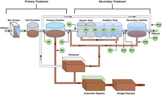
Figure 1.
WWTP with the data collection points along the waterline.
2.2. Framework
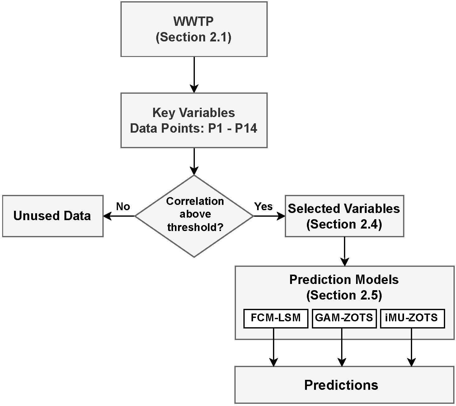
The proposed framework aims to develop a monitoring system for WWTPs based on the prediction of key variables in the treatment process. Data are collected at the WWTP from designated monitoring points (P1 to P14), as illustrated in Figure 1, and generated using the BSM2 simulator, which ensures no missing values. To increase the fidelity of the sensor measurements, noise with known statistical characteristics was added to the measured data. These noisy signals were used directly by the models, without any form of noise filtering. All variables were normalized to the range to account for differences in magnitude and to improve the performance of the machine learning models. Each collected (input) variable is analyzed for its correlation with the key process variables (targets). If the correlation exceeds a predefined threshold, the variable is selected for use in the predictive algorithms. These selected variables are then used to construct datasets for training and testing forecasting models. The prediction models are based on fuzzy systems that are employed to enhance the accuracy and interpretability of the forecasts. Figure 2 illustrates the sequence of the main steps, from data collection at the WWTP to the prediction of key variables performed by the fuzzy models.

Figure 2.
Flowchart of the proposed monitoring framework.
2.3. Key Variables and Prediction Points
For this study, the selected variables to be predicted (targets) are total suspended solids, [g/m3], ammonia and ammonium, [g N/m3], dissolved oxygen, [g /m3], nitrate and nitrite, [g N/m3], biological oxygen demand, [g/m3], and chemical oxygen demand, [g/m3].
The selection of these variables is justified by their significance in wastewater treatment processes. serves as a critical indicator of the removal efficiency of solid particles from wastewater. and must be closely monitored to assess the effectiveness of nitrogen compound removal. levels are essential for maintaining biological treatment processes, as they directly influence the activity of microorganisms. represents the concentration of biodegradable organic matter in wastewater, whereas quantifies the total organic load, including both biodegradable and non-biodegradable fractions [15].
Data collection was conducted at 14 points along the waterline, as shown in Figure 1:
- The prediction of is performed at the exit of the primary clarifier (P3) using data from P1 and P2 as input.
- is predicted at three locations: P3 (using P1 and P2), P10 (using P4 and P6), and P13 (using P11 and P12).
- is predicted at P10 with inputs from P4 and P6.
- is estimated at P3 (using P1 and P2), at P10 (using P4 and P6), and at the secondary clarifier outlet (P13, using P11 and P12).
- and are both predicted at P13 using data from P11 and P12.
In total, ten variables are predicted across different points in the wastewater treatment plant, with the collection points indicated in parentheses: , , , , , , , , and .
2.4. Selection of Input Variables
The input variables were selected based on their correlation with the target variables (key variables to be predicted). For that purpose, Pearson’s correlation is used. It measures the linear dependency between two variables, i.e., a given input variable () and the key variable Y, providing an indicator (r) about the strength of their relationship. The Pearson’s correlation r between variables and Y is given by [16]:
where and are the arithmetic means of and Y, respectively. and are the values of and Y at sample k, respectively, and K is the total number of samples.
Each input variable’s correlation with the target variable was evaluated against a predefined set of thresholds. Variable correlations exceeding a given threshold () were selected as input variables to be used in the prediction model. Multiple thresholds were considered, allowing for the selection of different input variables depending on the correlation values.
2.5. Fuzzy Models
Fuzzy logic systems (FLS) are rule-based systems defined with sets of fuzzy IF-THEN rules, where each rule has an IF statement (the antecedent part) and a THEN statement (consequent part), expressing high interpretability with the transformation of a human knowledge base into mathematical formulations [17]. Employing fuzzy-based models to create prediction models of the key variables on WWTPs offers several benefits for improving these processes, including addressing their uncertainty, complexity, and variability, as well as the creation of easy-to-understand frameworks. The following sections describe the fuzzy models implemented in this study.
2.5.1. Fuzzy Model Designed Using FCM and LSM
This model, named here as the FCM-LSM model, combines the fuzzy c-means (FCM) clustering method for the design of the antecedent part of the rules, and the least-squares method (LSM) for the design of the consequent part. The resulting model has the structure of a first-order Takagi-Sugeno (T-S) fuzzy system, whose rules are defined below [18]:
where
and the antecedent IF part from the i-th fuzzy rule () comprises the mapping of input variables using linguistic terms (). The i-th output of the consequent THEN from in Equation (2) is a function depending on model parameters and the predictor’s vector at k-th sample ().
FCM partitions a given dataset into N clusters (corresponding also to N fuzzy rules) or subsets characterized by membership values , with the aim of minimizing an objective function J [19]:
where m is the fuzzification degree, and is the square of the Euclidean distance (-norm) between sample and center of i-th cluster :
The optimal membership values are calculated as [19]:
and the center of i-th cluster is updated as follows:
The membership functions (MFs) in the final FCM-LSM model are represented by Gaussian functions, computed with the updated centers in Equation (8) and standard deviations , which are obtained as follows:
Antecedent Gaussian MFs, , and their normalized versions, , are calculated as follows:
The FCM-LSM output is obtained as the sum of the individual contributions of each rule from Equation (2):
and its global version can be computed as follows:
The consequent parameters are obtained by implementing LSM in Equation (13) considering the desired real output in place of [20]:
where when .
2.5.2. GAM-ZOTS
The GAM-ZOTS model consists of an approach for learning neo-fuzzy neuron systems, called generalized additive models using zero-order T-S fuzzy systems (GAM-ZOTS) [13]. The GAM-ZOTS structure consists of the sum of univariate models, whose fuzzy rules are expressed as follows:
where () is the -th rule for the j-th input variable. The linguistic terms define the MFs , and output is a function dependent of consequent parameters . The univariate model is defined as follows:
where is the normalized MF given by the following:
The global output of GAM-ZOTS is given by the following:
where is the model bias. The MFs from GAM-ZOTS are complementary triangular functions [21], defined a priori by fixing the number of rules for each univariate model, totaling global rules. Finally, the learning of the consequent parameters goes through the Backfitting Algorithm [22]. More details of the GAM-ZOTS model are presented in [13].
2.5.3. iMU-ZOTS
The iterative learning of multiple univariate zero-order T-S fuzzy systems (iMU-ZOTS) is the extension of GAM-ZOTS applied to the antecedent part [13]. Unlike GAM-ZOTS, which fixes the number of rules, iMU-ZOTS initializes with MFs (rules) for each input variable . Two complementary triangular MFs are defined considering the minimum and maximum values of as centers. Each sample () is evaluated to determine whether it is well represented by the existing fuzzy rules, using the following novelty detection mechanism:
where is the center of -th MF for j-th input variable from previous instant .
The creation of new rules depends on two criteria defined to assess whether the candidate sample is well represented in the existing rules (Criterion 1) and whether it can be considered as the center of the new MF based on the nearest MF (Criterion 2).
Criterion 1 (Novelty detection).
To determine the affinity of candidate sample to the current model, the values of from Equation (22) are evaluated in the following criterion:
where is a threshold for . If , is well represented by current model. In case of , does not fit into any rules and is considered new.
Criterion 2 (Minimal distance).
To minimize overfitting due to rules that are closely similar to each other, the following criterion is defined to evaluate the distance between two nearest MFs:
where is the center of the candidate MF (to be added) and is the center of its nearest MF. The threshold determine the minimal distance for the rule to be considered new, and can be defined based on the maximum amount of MFs, , allowed for input .
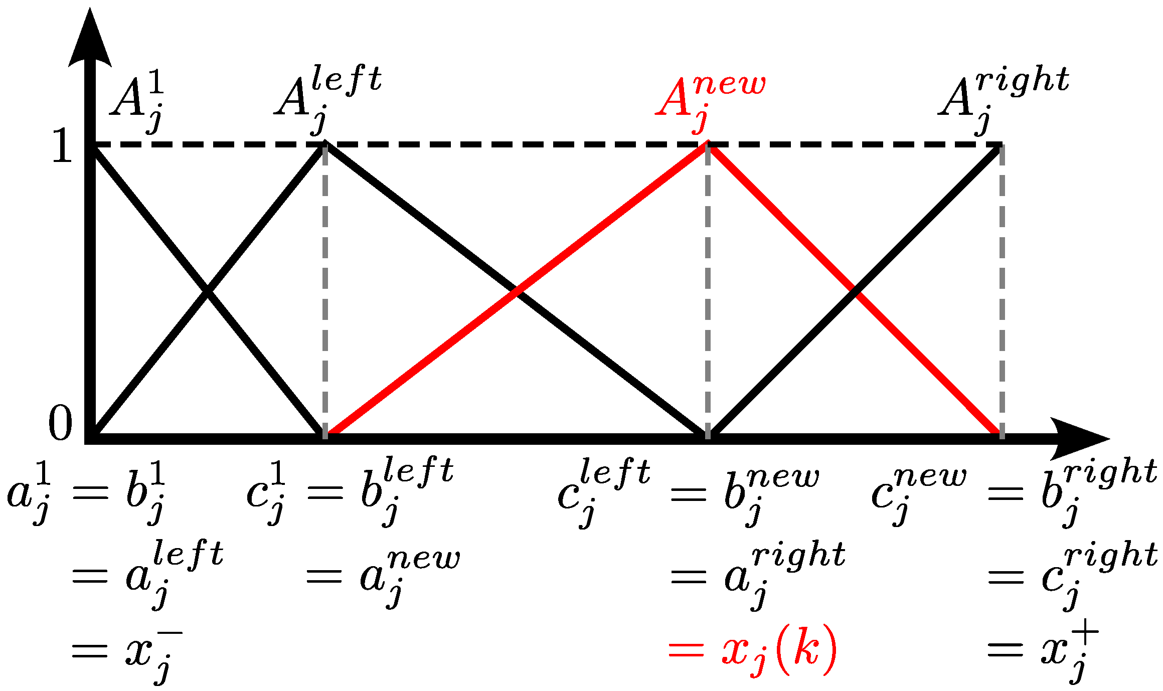
A new fuzzy rule is created (), with its respective MF , when Criteria 1 and 2 are met. Thus, the parameters of the new MF, as well as those of the two adjacent MFs and , are updated following the example shown in Figure 3.
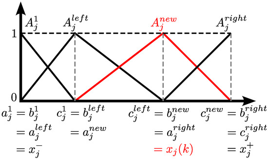
Figure 3.
Example of adding a new MF during learning of the iMU-ZOTS model.
Before proceeding to the next samples, the centers of the existing MFs are updated as follows:
where is the fuzzification degree, and indicates the accumulation of MFs until k-th sample associated to , with . More details of iMU-ZOTS model are presented in [13].
2.6. Proposed Framework Algorithm
Algorithm 1 outlines the setup of the proposed framework.
| Algorithm 1 Setup of the proposed framework. |
|
3. Results and Discussion
This section presents the results and the respective analyses regarding the accuracy and interpretability of the models.
3.1. Experimental Setup
The fuzzy methods were implemented using {MATLAB, version R2023b, where FCM-LSM was developed from scratch, and for the GAM-ZOTS and iMU-ZOTS models, their respective toolboxes were used (GAM-ZOTS and iMU-ZOTS toolboxes: https://www.jeromemendes.com/software, accessed on 20 March 2025). The parameters of the GAM-ZOTS and iMU-ZOTS models were chosen according to the ones tested in the original works that proposed these models and according to other works that use these models. Similarly, it was chosen for the FCM-LSM model, following the values commonly used in the literature. However, here we set up different combinations to determine the best configuration for each model by trial and error:
- FCM-LSM: number of clusters and fuzzification degree .
- GAM-ZOTS: number of fuzzy rules used , maximum number of iterations , and termination condition .
- iMU-ZOTS: , (for , , maximum number of iterations , termination condition , and fuzzification degree .
For the development of the proposed work, the Benchmark Simulator Model 2 (BSM2) [23] was used. The BSM2 is a simulation environment defining the plant layout, the simulation model, influence loads, test procedures, and evaluation criteria. The use of BSM2 is widely accepted by the scientific community and has already been used in several studies, such as optimization processes [24], variable prediction [25], and process control [26]. For the evaluation of the proposed framework, to predict each desired variable, 609 days are considered, where the first 245 days are used for stabilization of the plant. The sampling frequency is 15 min, totaling 58464 samples.
As mentioned in Section 2.4, each input variable’s correlation with the target variable was evaluated against a predefined set of thresholds. The following thresholds were defined: . The Pearson correlation thresholds adopted in this study were chosen due to their frequent use in the literature to represent different levels of association between variables [27], and are based on [28]. This gradation allows for a progressive analysis of the correlation between input variables and the target variable to be predicted. Variable correlations exceeding a given threshold () were selected as input variables to be used in the prediction model. As a result, four datasets were constructed for each predicted variable (one for each ), except for the variables and , where it was only possible to build two datasets since there were no input variables with a correlation above the predefined threshold. A total of 36 datasets were generated and evaluated across different models. For training and testing, each dataset was partitioned into 70% for training and 30% for testing.
3.2. Results
The results were evaluated through the Mean Squared Error (MSE) metric, described by the following Equation (27), where and are the real and estimated target at the instant of time k, and K is the total number of samples.
Table 1 presents the prediction results and interpretability of the different models for each dataset. The best MSE results are shown in the columns, where column represents the average MSE value. The optimal number of fuzzy rules, presented in column N, is highlighted in bold.

Table 1.
Results of the tests conducted with the three models. denotes the target variable, while represents the correlation threshold value. is the best error value for each dataset and represents the average prediction error () of each model. n indicates the number of input variables using the respective correlation threshold. N corresponds to the number of fuzzy rules used, and refers to the average number of fuzzy rules applied. represents the threshold value used by the iMU-ZOTS model. The best error value results for the models and the N values are highlighted in bold, whereas the best results for the other models are underlined.
Considering the MSE error values presented, it is evident that the FCM-LSM method achieved the lowest error values for nine variables, while the iMU-ZOTS method exhibited the best performance for only one variable, . Consequently, it can be concluded that FCM-LSM is the most effective method, producing the lowest MSE error for the majority of variables.
The correlation threshold value, represented in column , is a key parameter in this study, as it determines the selection of input variables used to construct the model. Four different threshold values were tested, and the results showed that as the threshold increased, the number of selected variables (column n) decreased, showing an inversely proportional relationship. Upon analyzing the results, it becomes clear that the best results are typically achieved when the threshold value is at its lowest, allowing the selection of more input variables and making the model more complex. Table 1 presents the number of fuzzy rules associated with the MSE results, along with the average rule count per method, which can be seen in column , and the threshold value at which the optimal results for the iMU-ZOTS method were achieved. The values corresponding to the best result are highlighted in bold, while the best results from the other two models are underlined.
The number of fuzzy rules used by each method is a key factor influencing model interpretability, which is particularly important for WWTP operators who require clear insights for decision-making. While accurate variable prediction is essential for efficient operation, helping to minimize resource waste and maintain water quality, model complexity can limit practical application. The analysis of Table 1 indicates that FCM-LSM achieves the lowest MSE values for most variables but relies on a high number of rules, and the model presents a much higher complexity on the antecedent and consequent parts, making it a less interpretable model. Therefore, achieving a balance between accuracy and interpretability is crucial for developing effective and practical models.
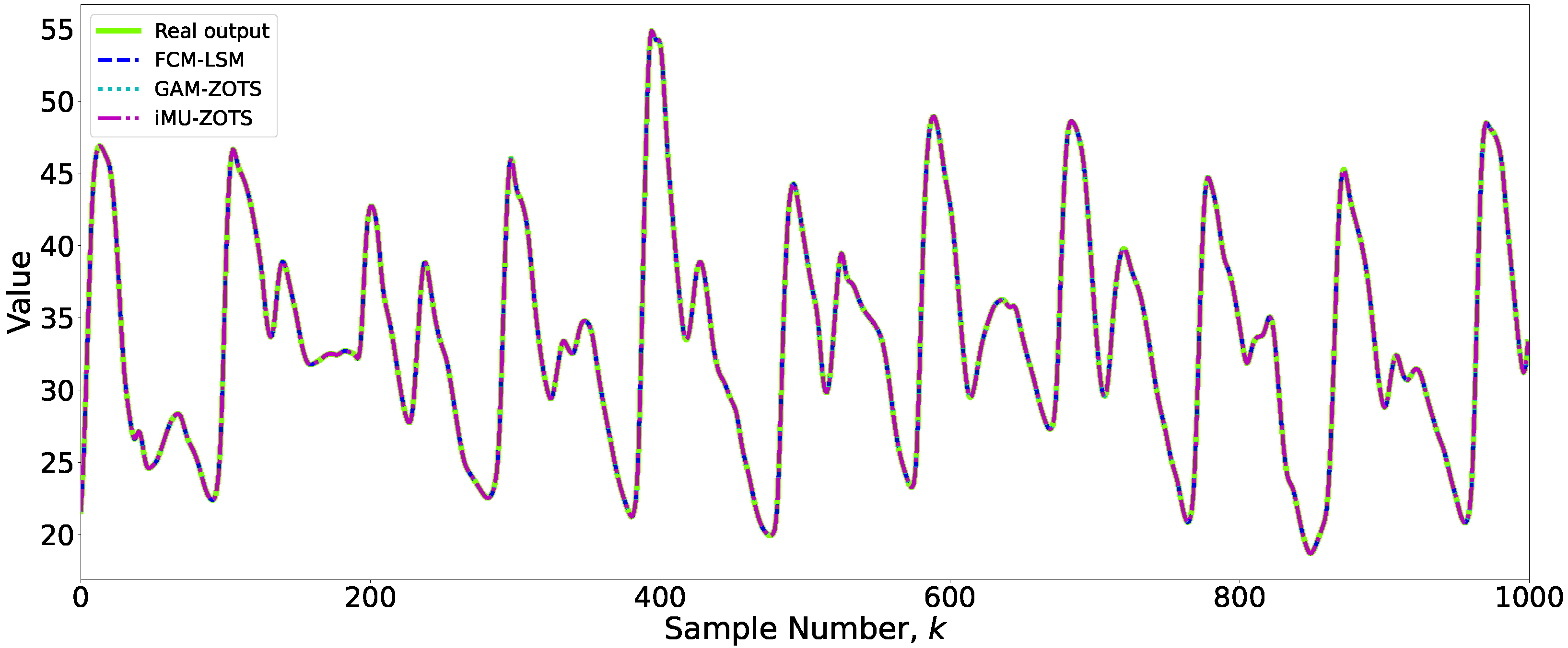
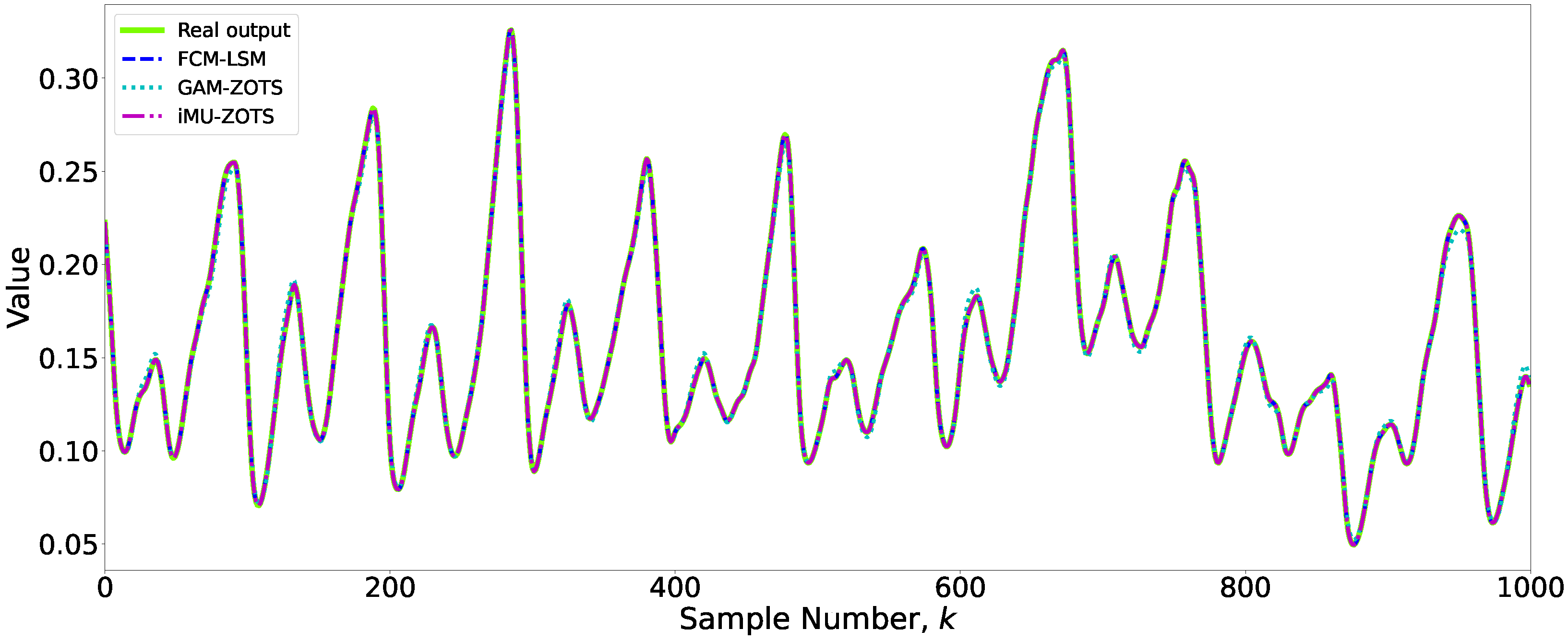
The optimal results obtained by the three methods were analyzed to assess both the accuracy and interpretability of the models. Additionally, methods that did not achieve the lowest error for each variable were considered, emphasizing the tradeoff between interpretability and accuracy. A simpler model, characterized by fewer rules, was preferred if its error rate remained reasonably close to the best value achieved for a given variable. To conduct a more detailed analysis of this balance, two variables, and , were selected as case studies. For , a threshold value of 0.85 was applied to the FCM-LSM and GAM-ZOTS methods, while a threshold of 0.5 was used for iMU-ZOTS. For , the threshold values varied across methods: 0.85 for FCM-LSM, 0.7 for GAM-ZOTS, and 0.3 for iMU-ZOTS. Figure 4 presents the prediction results for the variable obtained using the different methods.
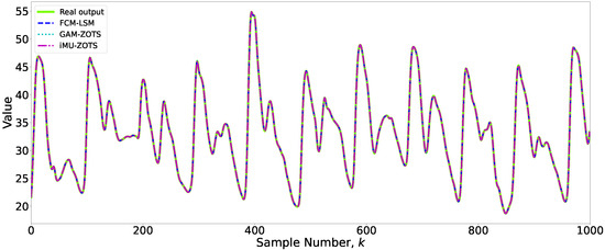
Figure 4.
Prediction results for the variable .
3.3. Accuracy vs. Interpretability:
Figure 4 shows the prediction results of the fuzzy models used in this study for variable .
An analysis of Figure 4 reveals that the differences in predictions among the various methods are minimal, with no statistically significant discrepancies observed. Therefore, slightly less accurate models may be preferable if they have better interpretability.
3.3.1. FCM-LSM
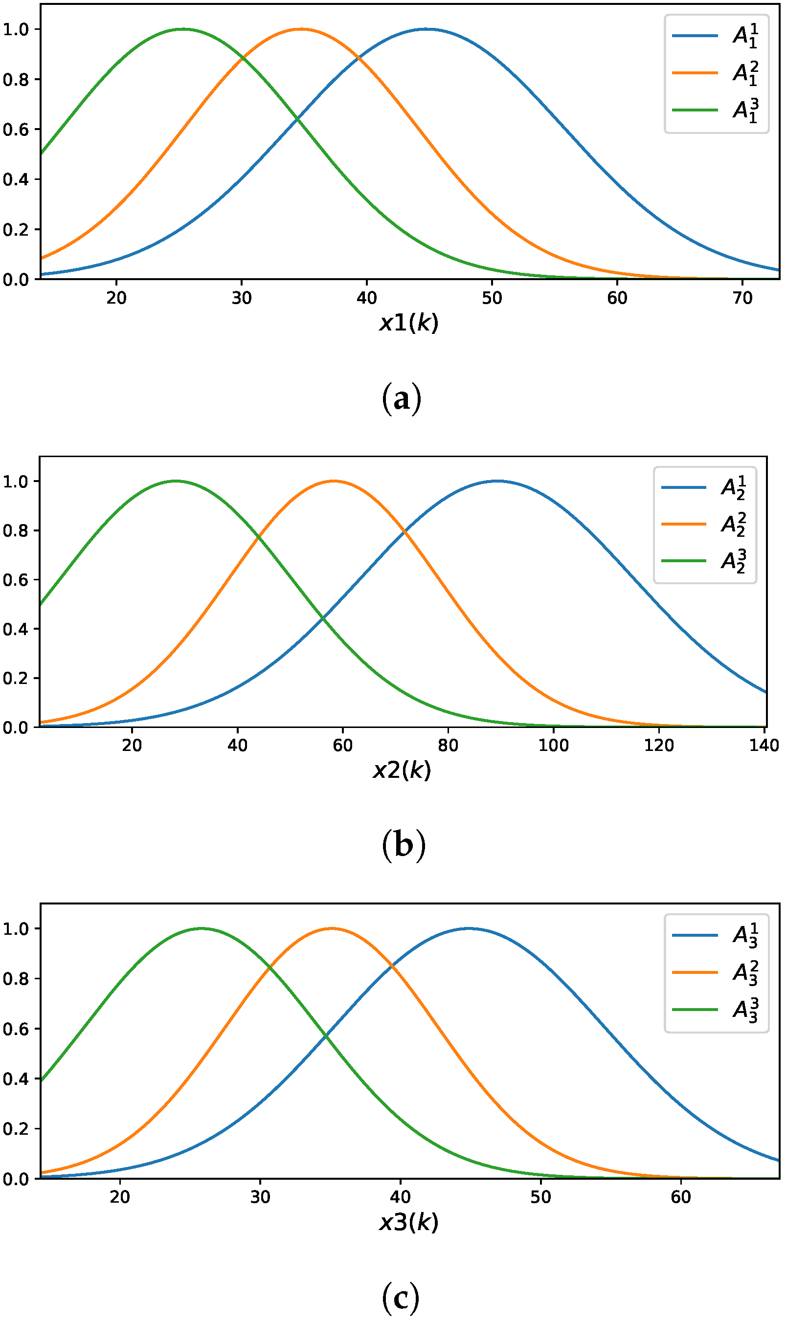
The FCM-LSM model learned for represents each of the three input variables using three fuzzy rules. Figure 5 illustrates the membership functions (MFs) associated with these input variables.
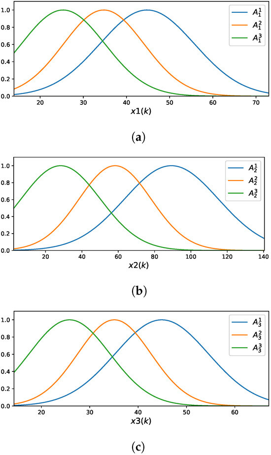
Figure 5.
Membership functions of the FCM-LSM for : (a) ; (b) ; (c) .
The fuzzy rules are described by the following:
- ,
- ,
- .
3.3.2. GAM-ZOTS
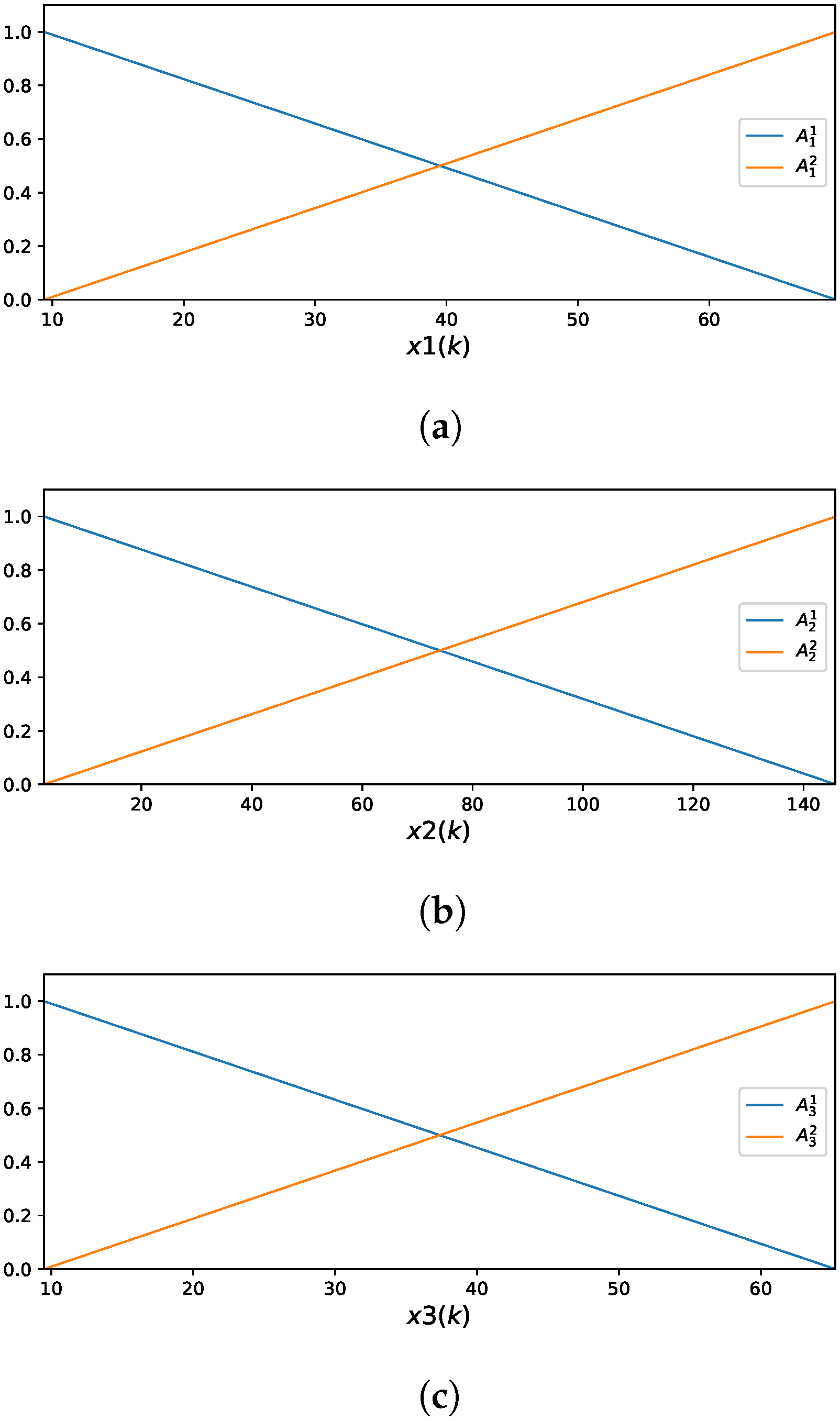
The GAM-ZOTS method represents each of the three selected input variables using two fuzzy rules. Figure 6 illustrates the MFs corresponding to these input variables.
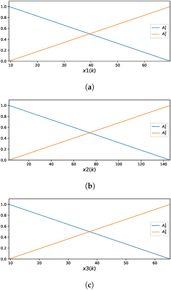
Figure 6.
Membership functions of the GAM-ZOTS for : (a) ; (b) ; (c) .
The fuzzy rules for the variable are defined as follows:
- ,
- ,
for the variable by
- ,
- ,
and for the variable by
- ,
- .
3.3.3. iMU-ZOTS
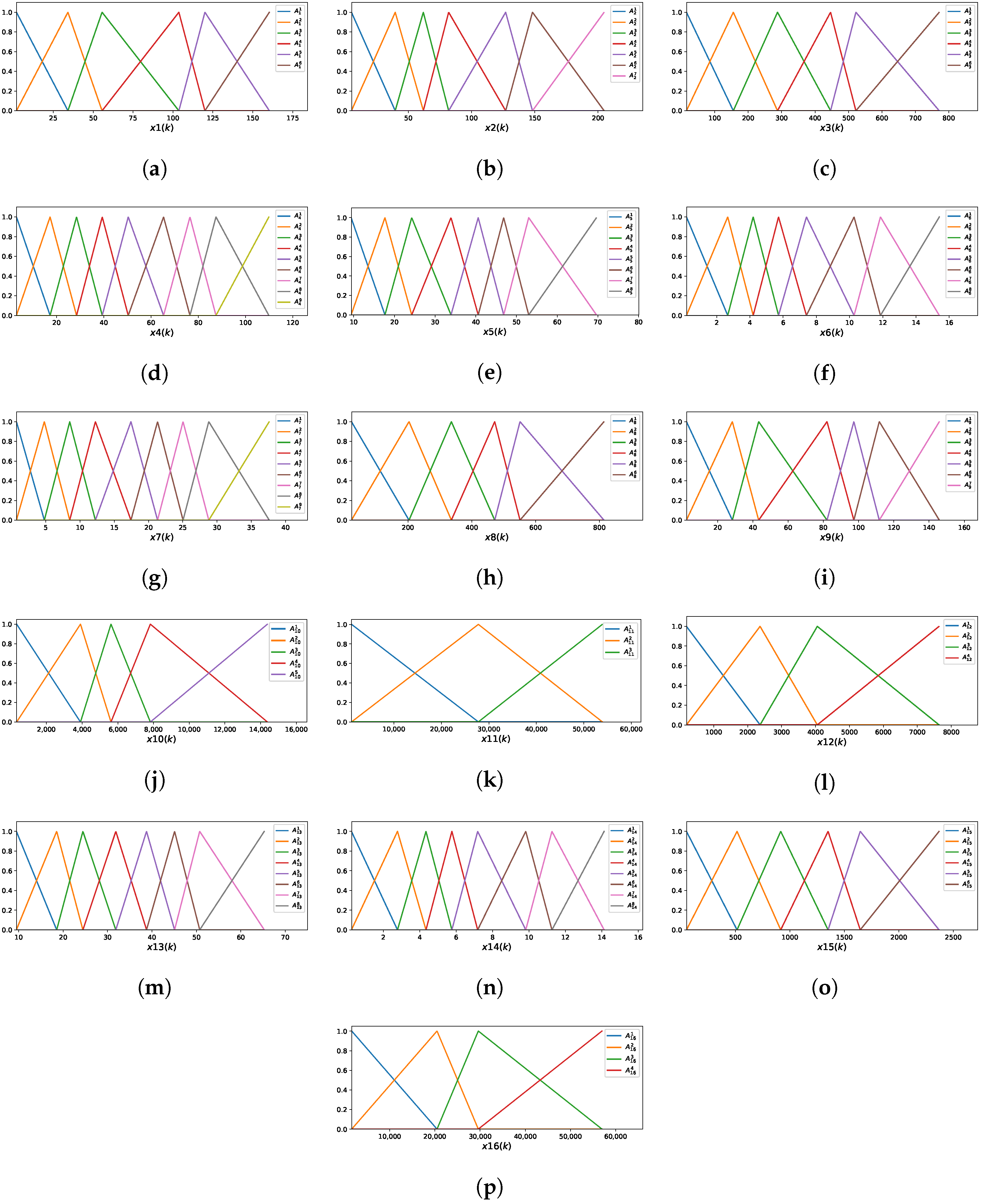
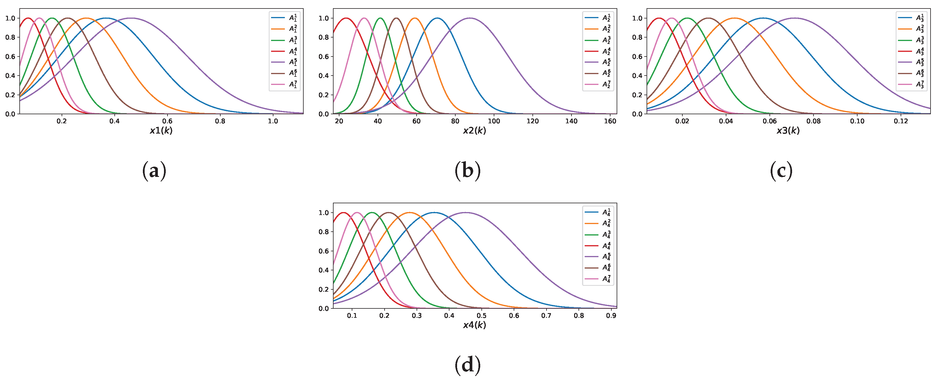
The optimal model using the iMU-ZOTS method is characterized by 16 selected input variables, with an average of 6.5 fuzzy rules per variable, calculated as the total number of fuzzy rules divided by the number of input variables. The model comprises a total of fuzzy rules, with each of the 16 variables contributing the following number of rules: , , , , , , , , , , , , , , , and . Figure 7 presents the MFs for all 16 input variables. Due to the large number of rules and space constraints, the rules of the iMU-ZOTS method are not described here.
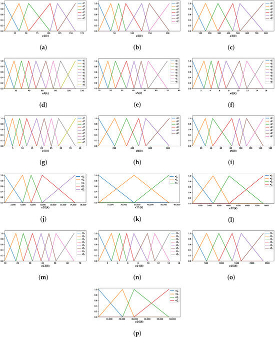
Figure 7.
Membership functions of the iMU-ZOTS method for the variable : (a) ; (b) ; (c) ; (d) ; (e) ; (f) ; (g) ; (h) ; (i) ; (j) ; (k) ; (l) ; (m) ; (n) ; (o) ; (p) .
3.4. Accuracy vs. Interpretability:
Another analyzed variable is . Figure 8 presents the prediction results for obtained using the three methods.
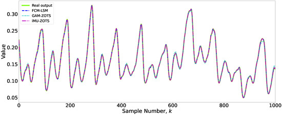
Figure 8.
Prediction results for the variable .
All methods produce comparable results with no significant differences in accuracy, indicating that any of them can achieve reliable performance. Consequently, evaluating interpretability becomes essential, which requires analyzing the number of fuzzy rules employed by each method.
3.4.1. FCM-LSM
The learned FCM-LSM model is characterized by four input variables and a set of seven fuzzy rules. Figure 9 presents the MFs corresponding to the four input variables.
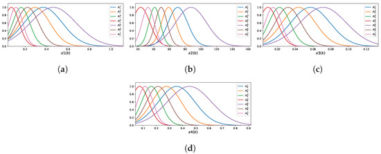
Figure 9.
Membership functions of the FCM-LSM for : (a) ; (b) ; (c) ; (d) .
The fuzzy rules are described by the following:
- ,
- ,
- ,
- ,
- ,
- ,
- .
3.4.2. GAM-ZOTS
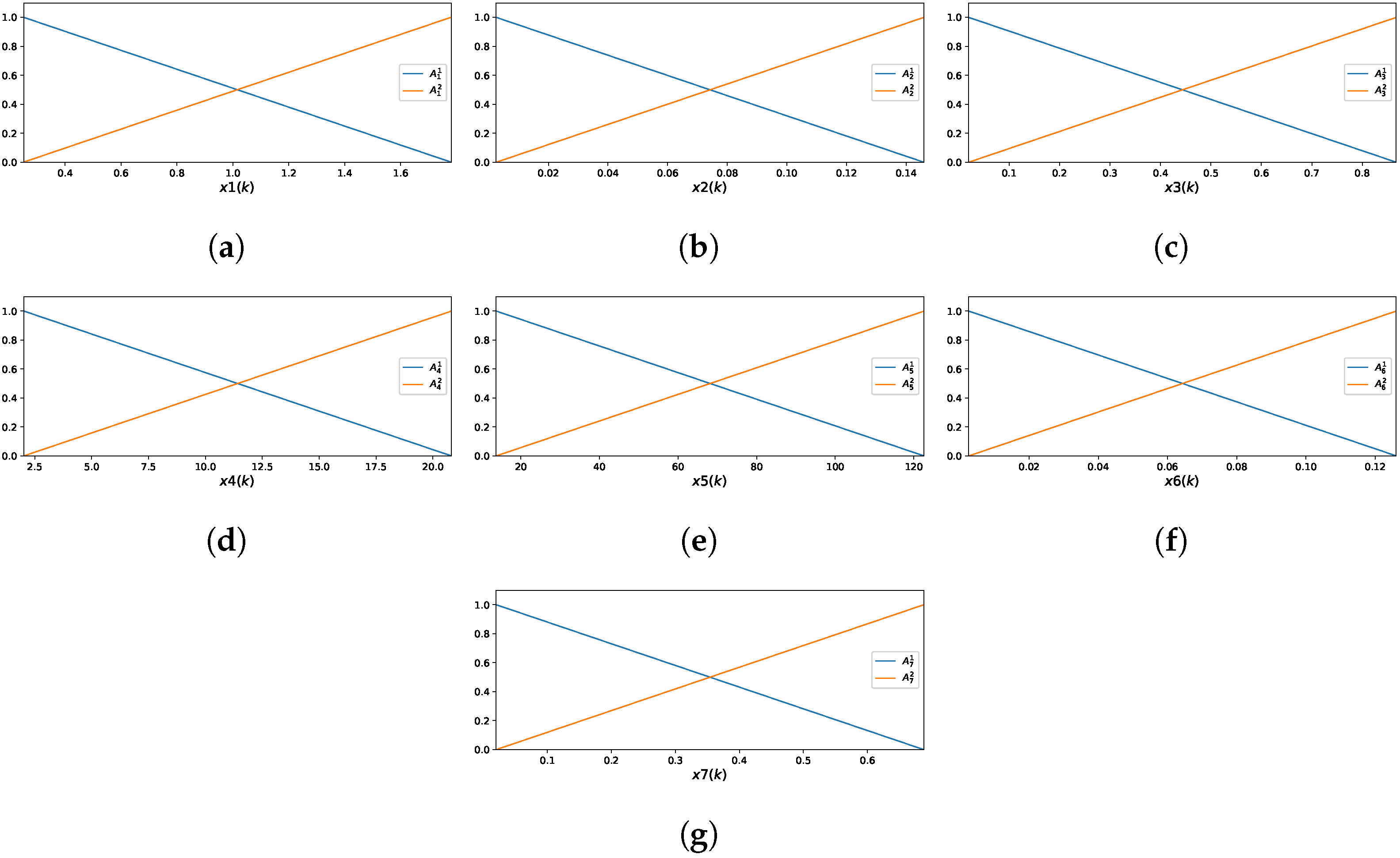
The GAM-ZOTS method represents each of the seven selected input variables using two fuzzy rules. Figure 10 illustrates the MF corresponding to these input variables.
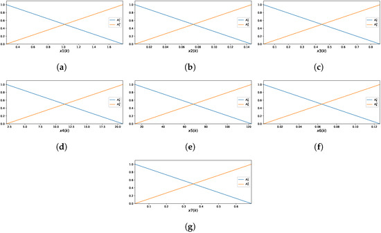
Figure 10.
Membership functions of the GAM-ZOTS for : (a) ; (b) ; (c) ; (d) ; (e) ; (f) ; (g) .
The fuzzy rules for the variable in the GAM-ZOTS model are defined as follows:
- ,
- ,
for the variable by
- ,
- ,
for the variable by
- ,
- ,
for the variable by
- ,
- ,
for the variable by
- ,
- ,
for the variable by
- ,
- ,
and for the variable by
- ,
- .
3.4.3. iMU-ZOTS
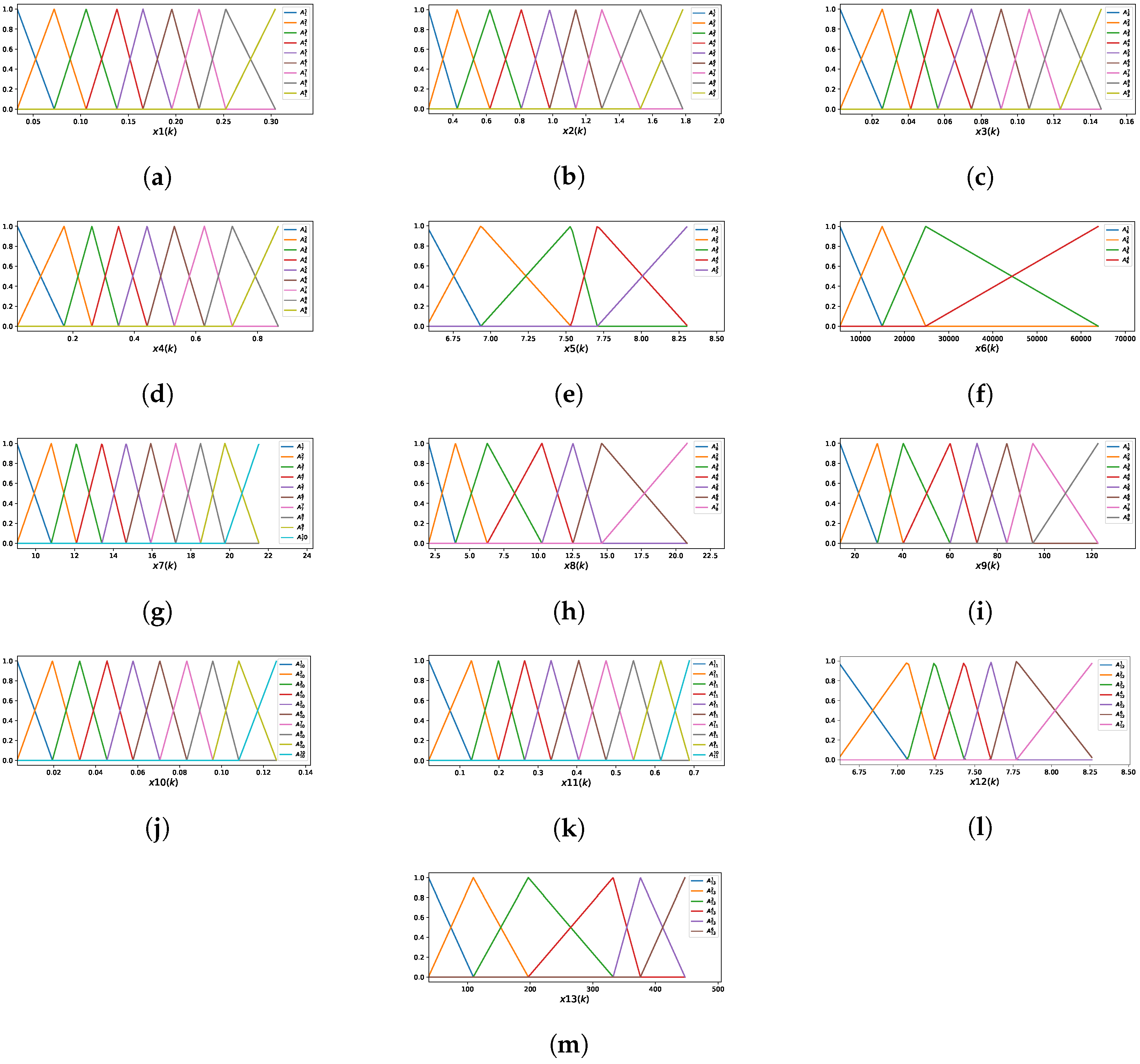
The iMU-ZOTS model is characterized by 13 selected input variables, with an average of 7.92 fuzzy rules per variable. This average is calculated by dividing the total number of rules across all variables by the number of variables. The model consists of a total of fuzzy rules, distributed as follows: , , , , , , , , , , , and . Figure 11 illustrates the membership functions for the 13 input variables. Due to the large number of rules and the limited space available, the rules are not described here.
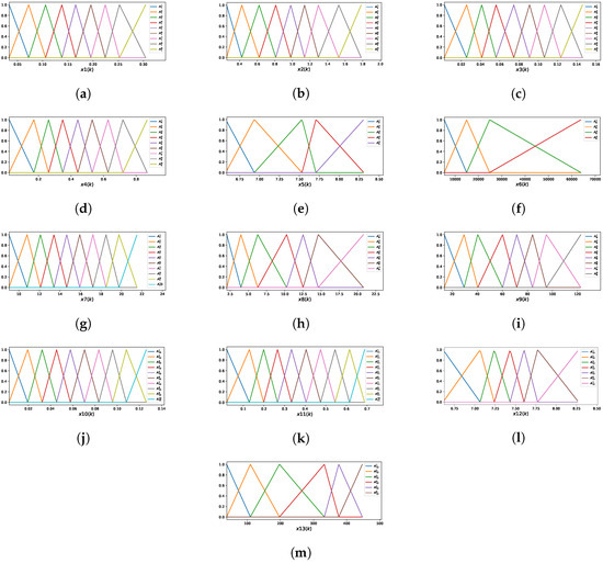
Figure 11.
Membership functions of the iMU-ZOTS for : (a) ; (b) ; (c) ; (d) ; (e) ; (f) ; (g) ; (h) ; (i) ; (j) ; (k) ; (l) ; (m) .
3.5. Accuracy vs. Interpretability: Discussion
After analyzing the results for the two target variables, it is evident that although the FCM-LSM method exhibits a lower error value compared to the other methods, the difference in prediction accuracy is minimal. Additionally, FCM-LSM delivers the best results, although with more complex rules than the other methods. Models with a high number of rules, a high number of membership functions, or numerous input variables in the antecedent part tend to be more complex and challenging for operators to interpret. In the context of WWTPs, operators need to understand the models easily in order to make informed decisions throughout the treatment process. An industrial process model is better when it is interpretable, allowing engineers, operators, and decision-makers to understand how and why the model is making predictions or recommendations. An interpretable system, built on familiar linguistic terms, enables operators to build trust in the model’s recommendations, which in turn facilitates rapid identification of equipment malfunctions and process anomalies and strengthens confidence in the data that support decision-making (troubleshooting and diagnostics). Moreover, operators and engineers are more likely to validate, trust, and adopt a model if they can understand its logic, especially in industrial environments. And interpretable models help encode and transfer process knowledge across teams and generations of workers. By tracing each action back to a small set of human-readable rules, operators can quickly diagnose faults, adjust settings, and ensure that plant operations remain both compliant with environmental regulations and aligned with sustainability goals. In this context, GAM-ZOTS and iMU-ZOTS are more advantageous than FCM-LSM because they have rules with univariable antecedents, allowing the operators to analyse the individual impact of each input variable on the key variables. However, iMU-ZOTS provided greater variability in the number of rules for each input, which increased its overall complexity.
For the variable , the FCM-LSM method obtains an MSE value of with 3 associated fuzzy rules. GAM-ZOTS produces an , higher than the FCM-LSM error, using two univariate fuzzy rules per variable. Meanwhile, iMU-ZOTS results in an MSE of , higher than the FCM-LSM error, and 6.5 fuzzy rules per variable. Since the predictions made by all three methods are identical (as shown in Figure 4), the method with the least complexity should be preferred. In this case, GAM-ZOTS is the best choice for this variable. However, FCM-LSM could also be a viable option due to its lower error and fewer fuzzy rules.
For the variable, FCM-LSM achieves an MSE of with 7 fuzzy rules. In comparison, GAM-ZOTS produces an MSE of , which is higher than the FCM-LSM error, with 2 fuzzy rules per variable. The iMU-ZOTS method produces an MSE of , which is higher than FCM-LSM, with an average of 7.92 fuzzy rules per variable. Analysis of Figure 8 reveals that the differences in the predictions for this variable across the methods are minimal. Therefore, the most suitable method for this variable should be selected based on the model’s simplicity. In this case, GAM-ZOTS offers the best balance between prediction accuracy and interpretability, providing accurate results while remaining easy for operators to understand.
4. Conclusions
This study aimed to develop an interpretable digital monitoring system for key waterline variables in WWTPs. Through the use of fuzzy-based models, the proposed approach enhances process monitoring by providing a transparent and explainable framework for decision-making. The study compared three fuzzy-based models, evaluating their accuracy and interpretability, which are critical factors for practical implementation in WWTP operations. To construct the datasets, data were collected from 14 specific points along the waterline of the WWTP. These points were selected to capture essential process variables, ensuring comprehensive monitoring throughout the different treatment stages. The selected variables included , , , , , and . The datasets were built using distinct sets of input variables at each collection point, and the models were trained and tested to optimize both accuracy and interpretability. The results demonstrate that while FCM-LSM achieves the highest accuracy, its complexity limits its interpretability. On the other hand, GAM-ZOTS and iMU-ZOTS offer a better tradeoff between accuracy and simplicity, making them more suitable for real-world applications where interpretability is essential for operational decision-making. The findings highlight the importance of balancing predictive accuracy with model complexity to ensure that the models are more interpretable and the operators can effectively utilize the digital monitoring system. As future work, other machine learning models will be applied to the same dataset to assess whether alternative methods offer different results or advantages compared to fuzzy-based models. This could provide further insights into the robustness and applicability of the proposed framework.
Author Contributions
Methodology, R.S., M.P. and J.M.; Software, M.P.; Validation, R.S., M.P., R.A., J.S.S.J. and J.M.; Investigation, R.S. and M.P.; Writing—original draft, R.S., M.P. and J.S.S.J.; Writing—review and editing, R.S., R.A., J.S.S.J. and J.M.; Project administration, R.A. and J.M.; Supervision, R.A. and J.M. All authors have read and agreed to the published version of the manuscript.
Funding
Rodrigo Salles and Jorge S. S. Júnior are supported by Fundação para a Ciência e a Tecnologia (FCT) under the grant refs. 2023.01009.BD and 2021.04917.BD, respectively. This research is partially sponsored by national funds through FCT under projects UID/00285—Centre for Mechanical Engineering, Materials and Processes and LA/P/0112/2020.
Data Availability Statement
The original contributions presented in this study are included in the article. Further inquiries can be directed to the corresponding author.
Conflicts of Interest
The authors declare no conflicts of interest.
References
- Yang, F.; Gu, S. Industry 4.0, a revolution that requires technology and national strategies. Complex Intell. Syst. 2021, 7, 1311–1325. [Google Scholar] [CrossRef]
- Nakkasunchi, S.; Hewitt, N.J.; Zoppi, C.; Brandoni, C. A review of energy optimization modelling tools for the decarbonisation of wastewater treatment plants. J. Clean. Prod. 2021, 279, 123811. [Google Scholar] [CrossRef]
- Nguyen, T.; Ngo, H.; Guo, W.; Chang, S.; Nguyen, D.; Nghiem, L.; Nguyen, T. A critical review on life cycle assessment and plant-wide models towards emission control strategies for greenhouse gas from wastewater treatment plants. J. Environ. Manag. 2020, 264, 110440. [Google Scholar] [CrossRef] [PubMed]
- Cheng, H.; Wu, J.; Liu, Y.; Huang, D. A novel fault identification and root-causality analysis of incipient faults with applications to wastewater treatment processes. Chemom. Intell. Lab. Syst. 2019, 188, 24–36. [Google Scholar] [CrossRef]
- Yin, S.; Xie, X.; Sun, W. A nonlinear process monitoring approach with locally weighted learning of available data. IEEE Trans. Ind. Electron. 2016, 64, 1507–1516. [Google Scholar] [CrossRef]
- Mamandipoor, B.; Majd, M.; Sheikhalishahi, S.; Modena, C.; Osmani, V. Monitoring and detecting faults in wastewater treatment plants using deep learning. Environ. Monit. Assess. 2020, 192, 148. [Google Scholar] [CrossRef]
- Safder, U.; Kim, J.; Pak, G.; Rhee, G.; You, K. Investigating machine learning applications for effective real-time water quality parameter monitoring in full-scale wastewater treatment plants. Water 2022, 14, 3147. [Google Scholar] [CrossRef]
- Molnar, C. Interpretable Machine Learning; Lulu.com: Morrisville, NC, USA, 2020. [Google Scholar]
- Ferdaus, M.M.; Dam, T.; Alam, S.; Pham, D.T. X-Fuzz: An Evolving and Interpretable Neuro-Fuzzy Learner for Data Streams. IEEE Trans. Artif. Intell. 2024, 5, 4001–4012. [Google Scholar] [CrossRef]
- Zhao, H.; Wu, Y.; Deng, W. An Interpretable Dynamic Inference System Based on Fuzzy Broad Learning. IEEE Trans. Instrum. Meas. 2023, 72, 1–12. [Google Scholar] [CrossRef]
- Moral, A.; Castiello, C.; Magdalena, L.; Mencar, C. Explainable Fuzzy Systems; Springer: Berlin/Heidelberg, Germany, 2021. [Google Scholar] [CrossRef]
- Mendes, J.; Souza, F.; Araújo, R.; Rastegar, S. Neo-fuzzy neuron learning using backfitting algorithm. Neural Comput. Appl. 2019, 31, 3609–3618. [Google Scholar] [CrossRef]
- Mendes, J.; Souza, F.A.; Maia, R.; Araújo, R. Iterative Learning of Multiple Univariate Zero-Order TS Fuzzy Systems. In Proceedings of the IECON 2019-45th Annual Conference of the IEEE Industrial Electronics Society, Lisbon, Portugal, 14–17 October 2019; Volume 1, pp. 3803–3808. [Google Scholar] [CrossRef]
- European Parliament and Council of the European Union. Directive (EU) 2024/3019 of the European Parliament and of the Council of 27 November 2024 on Urban Wastewater Treatment. Off. J. Eur. Union 2024, 2024, 3019. [Google Scholar]
- Spellman, F.R. Handbook of Water and Wastewater Treatment Plant Operations; CRC Press: Boca Raton, FL, USA, 2008. [Google Scholar]
- Jebli, I.; Belouadha, F.Z.; Kabbaj, M.I.; Tilioua, A. Prediction of solar energy guided by pearson correlation using machine learning. Energy 2021, 224, 120109. [Google Scholar] [CrossRef]
- Júnior, J.S.S.; Mendes, J.; Souza, F.; Premebida, C. Survey on Deep Fuzzy Systems in Regression Applications: A View on Interpretability. Int. J. Fuzzy Syst. 2023, 25, 2568–2589. [Google Scholar] [CrossRef]
- Takagi, T.; Sugeno, M. Fuzzy identification of systems and its applications to modeling and control. IEEE Trans. Syst. Man Cybern. 1985, 1, 116–132. [Google Scholar] [CrossRef]
- Dovžan, D.; Škrjanc, I. Recursive fuzzy c-means clustering for recursive fuzzy identification of time-varying processes. ISA Trans. 2011, 50, 159–169. [Google Scholar] [CrossRef] [PubMed]
- Regattieri Delgado, M.; Von Zuben, F.; Gomide, F. Hierarchical genetic fuzzy systems. Inf. Sci. 2001, 136, 29–52. [Google Scholar] [CrossRef]
- da Silva Júnior, G.A.; da Silva, A.M. A simple and efficient incremental missing data imputation method for evolving neo-fuzzy network. Evol. Syst. 2022, 13, 201–220. [Google Scholar] [CrossRef]
- Hastie, T.J. Generalized additive models. In Statistical Models in S; Routledge: Oxfordshire, UK, 2017; pp. 249–307. [Google Scholar] [CrossRef]
- Jeppsson, U.; Pons, M.N.; Nopens, I.; Alex, J.; Copp, J.; Gernaey, K.; Rosen, C.; Steyer, J.P.; Vanrolleghem, P. Benchmark simulation model no 2: General protocol and exploratory case studies. Water Sci. Technol. 2007, 56, 67–78. [Google Scholar] [CrossRef]
- Roșu, B.; Mocanu, G.D.; Pila, M.M.; Murariu, G.; Roșu, A.; Arseni, M. Enhancing the Performance of a Simulated WWTP: Comparative Analysis of Control Strategies for the BSM2 Model. Mathematics 2023, 11, 3471. [Google Scholar] [CrossRef]
- Voipan, D.; Voipan, A.E.; Barbu, M. Evaluating Machine Learning-Based Soft Sensors for Effluent Quality Prediction in Wastewater Treatment Under Variable Weather Conditions. Sensors 2025, 25, 1692. [Google Scholar] [CrossRef]
- Liu, Y.; Zhang, J.; Qiu, Z.; Zhang, Y.; Yu, G.; Ye, H.; Cai, Z. Towards stable and efficient nitrogen removal in wastewater treatment processes via an adaptive neural network based sliding mode controller. Water Res. X 2024, 24, 100245. [Google Scholar] [CrossRef] [PubMed]
- Leiria, J.; Salles, R.; Mendes, J.; Sousa, P. Soft sensors for industrial applications: Comparison of variables selection methods and regression models. In Proceedings of the 2023 International Conference on Control, Automation and Diagnosis (ICCAD), Rome, Italy, 10–12 May 2023; pp. 1–6. [Google Scholar]
- Freedman, D.; Pisani, R.; Purves, R. Statistics; W. W. Norton & Company, Inc.: New York, NY, USA, 1998. [Google Scholar]

Disclaimer/Publisher’s Note: The statements, opinions and data contained in all publications are solely those of the individual author(s) and contributor(s) and not of MDPI and/or the editor(s). MDPI and/or the editor(s) disclaim responsibility for any injury to people or property resulting from any ideas, methods, instructions or products referred to in the content. |
© 2025 by the authors. Licensee MDPI, Basel, Switzerland. This article is an open access article distributed under the terms and conditions of the Creative Commons Attribution (CC BY) license (https://creativecommons.org/licenses/by/4.0/).