
Self-Evolving Chebyshev Radial Basis Function Neural Complementary Sliding Mode Control

Abstract
1. Introduction
- (1)
- The designed new CSMC algorithm is oriented to a multi-dimensional uncertain nonlinear system and does not depend on an accurate mathematical model. The superiority of the proposed method is explored to show that it has a smaller steady-state error.
- (2)
- A network combining the CN and the RBFNN is designed. The network combines the advantages of the CN and the RBFNN in function approximation and is not obvious in increasing the complexity of the algorithm. At the same time, the structure self-evolution mechanism is added to the network, so that the network structure can be adjusted according to the actual control scenario.
- (3)
- The SAPF model is adopted in the simulation phase. CSMC and the proposed method are respectively applied to the SAPF current control system. The comparative study between two methods is accomplished to highlight the superiority of the proposed method, from the perspectives of current tracking, harmonic compensation, and network operation time.
2. Problem Statement and Preliminaries
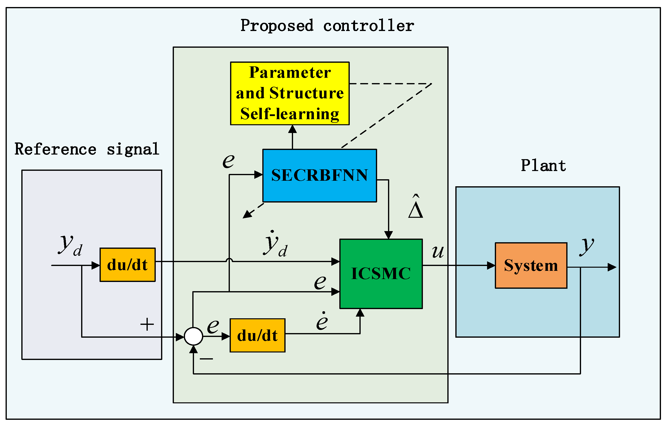
3. Proposed Control Method and Stability Verification
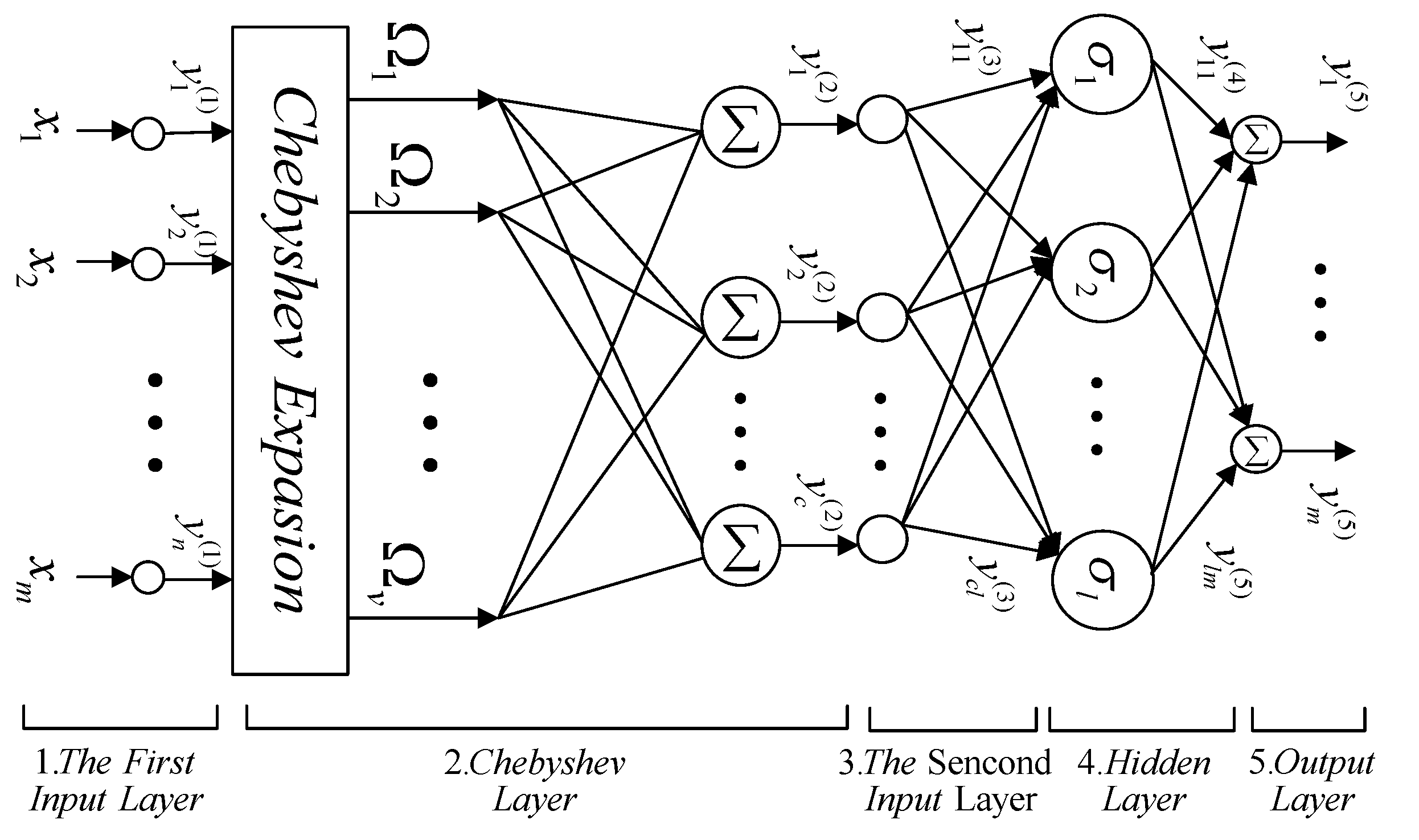
3.1. Structure of the Self-Evolving Chebyshev Radial Basis Function Neural Network
- (1)
- Layer 1—the first input layer: This layer is used to transfer the input signal. For each node, the relationship between the output and input are as follows:
- (2)
- Layer 2—Chebyshev layer: Chebyshev polynomials are used to map the NN input to a higher dimensional space. In the high-dimensional space, the input signals can be divided as:
- (3)
- Layer 3—the second input layer: This layer is the bridge between the CNN and the RBFNN. The output is expressed as:
- (4)
- Layer 4—hidden layer: The mapping of input signals in this layer is the key to the performance of the RBFNN [35]. The output of this layer can be expressed as:
- (5)
- Layer 5—output layer: This layer is used to transport the output signal of the entire network. The expression of the output of this layer is as follows:
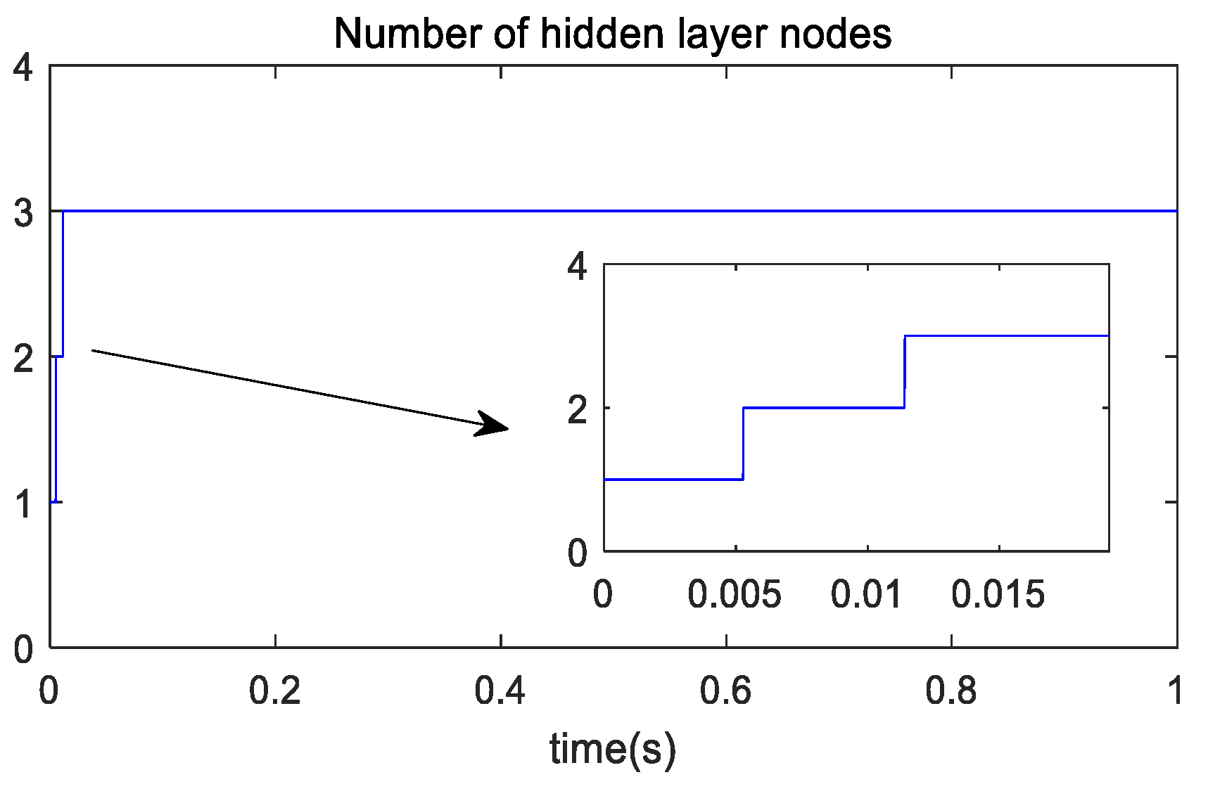
3.2. Self-Evolving Mechanism
3.3. Controller Design and Stability Proof
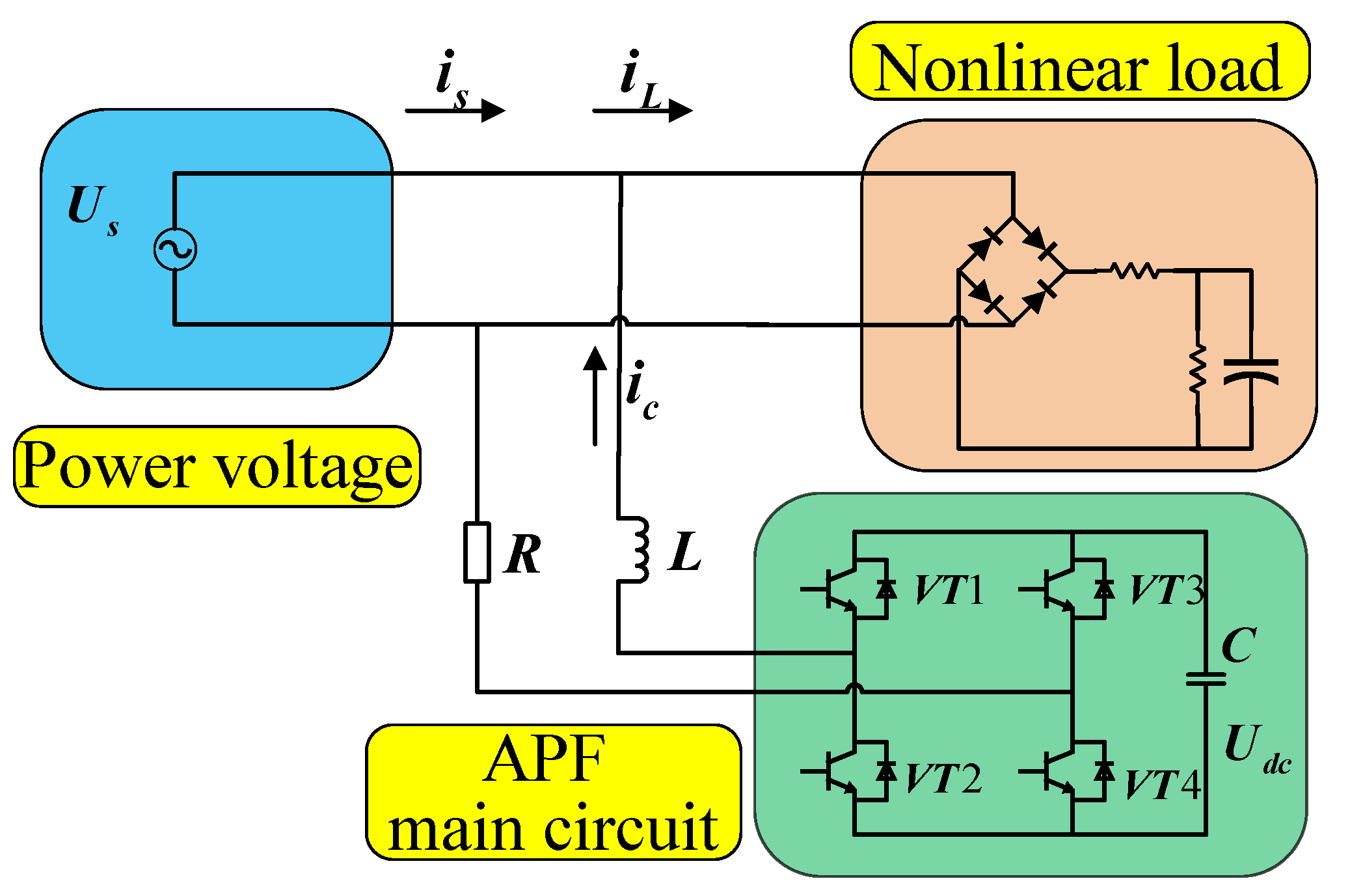
4. Simulation Study
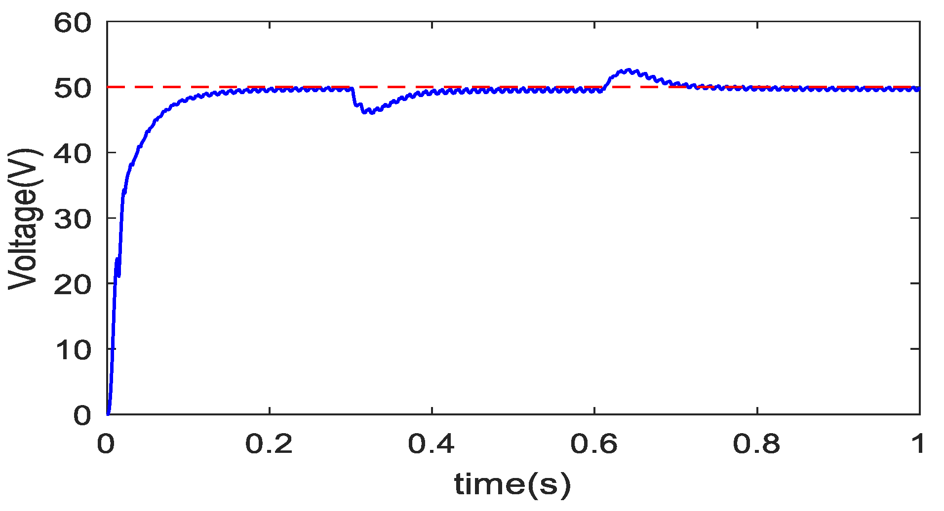
4.1. Introduction of the Model and Parameters
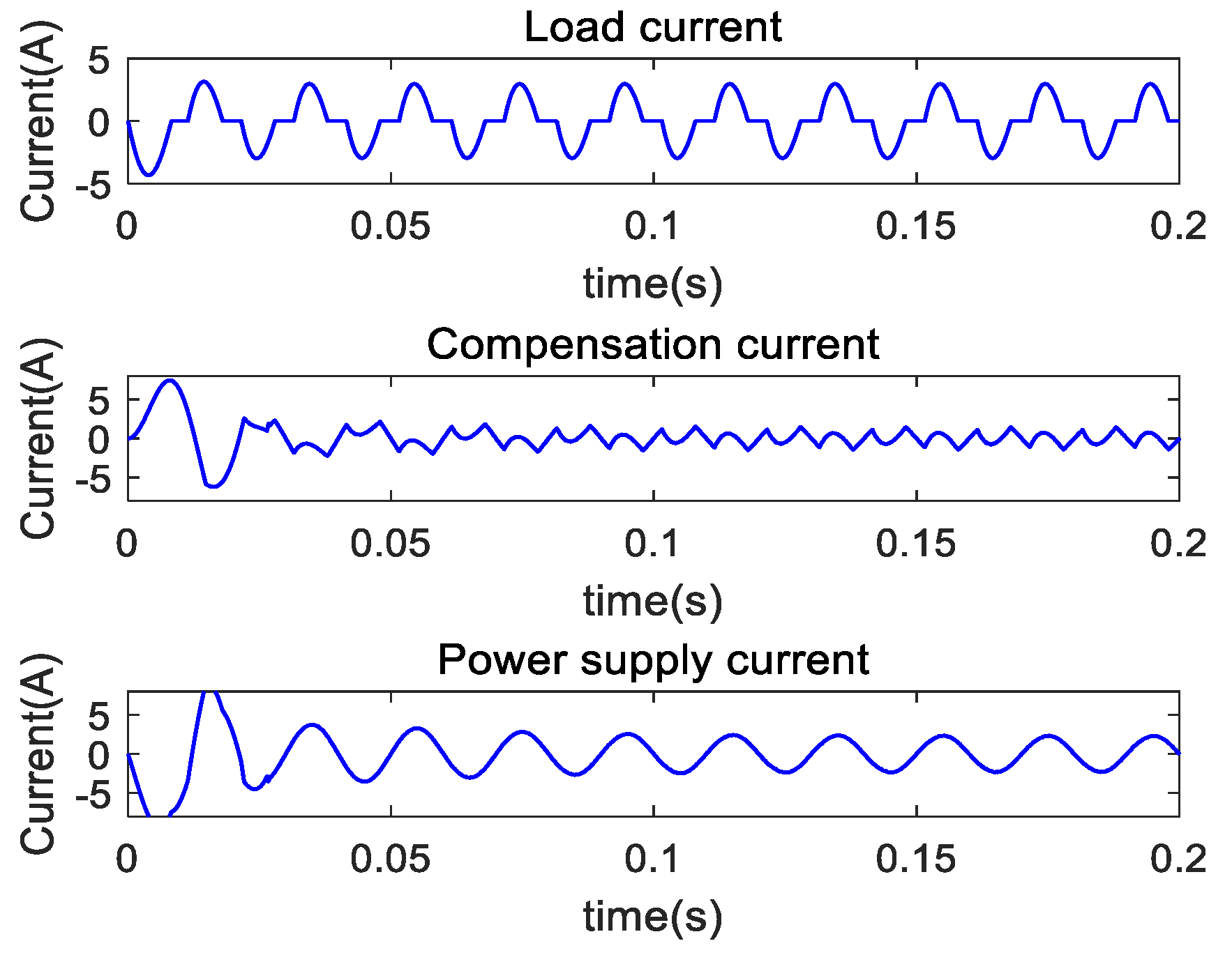
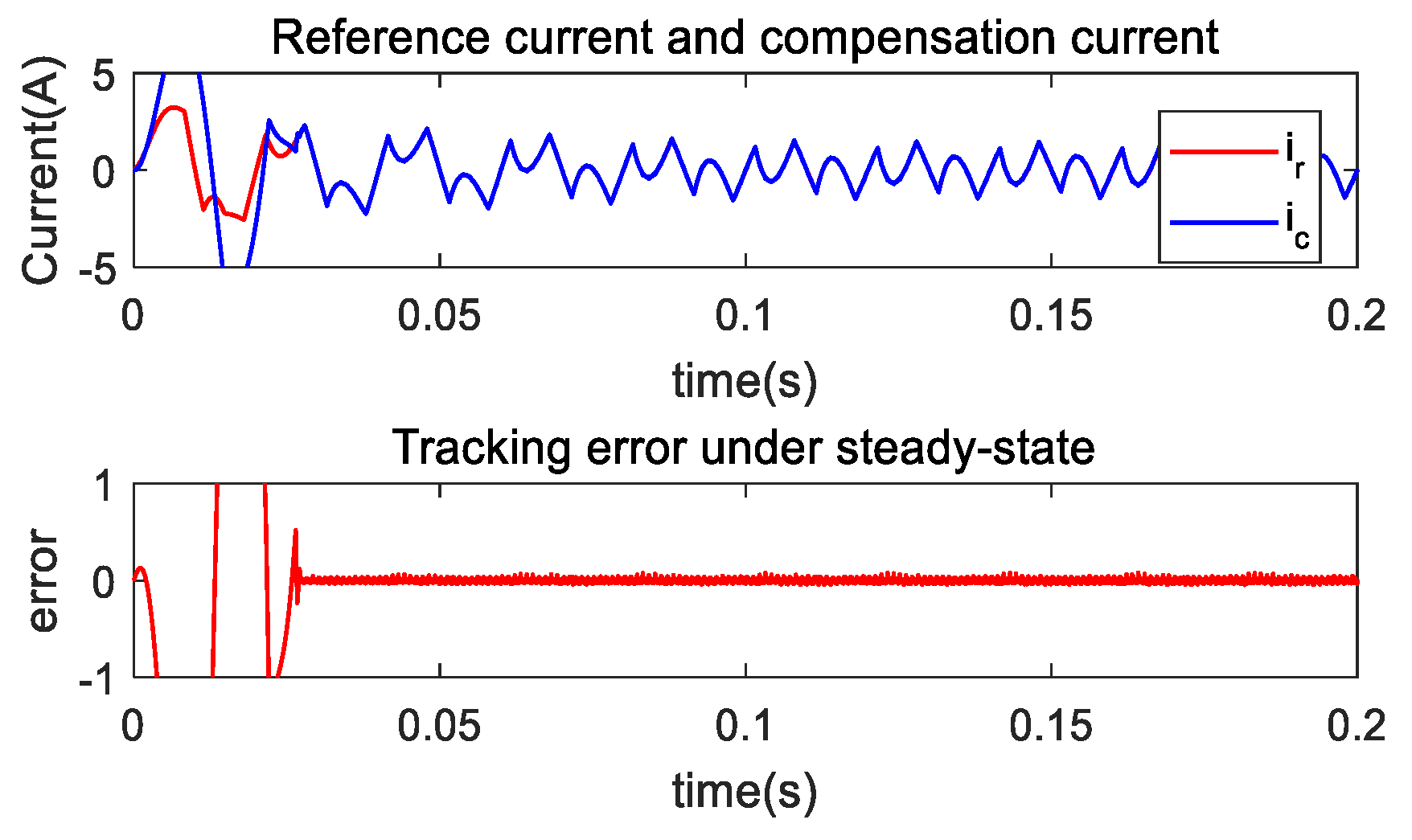
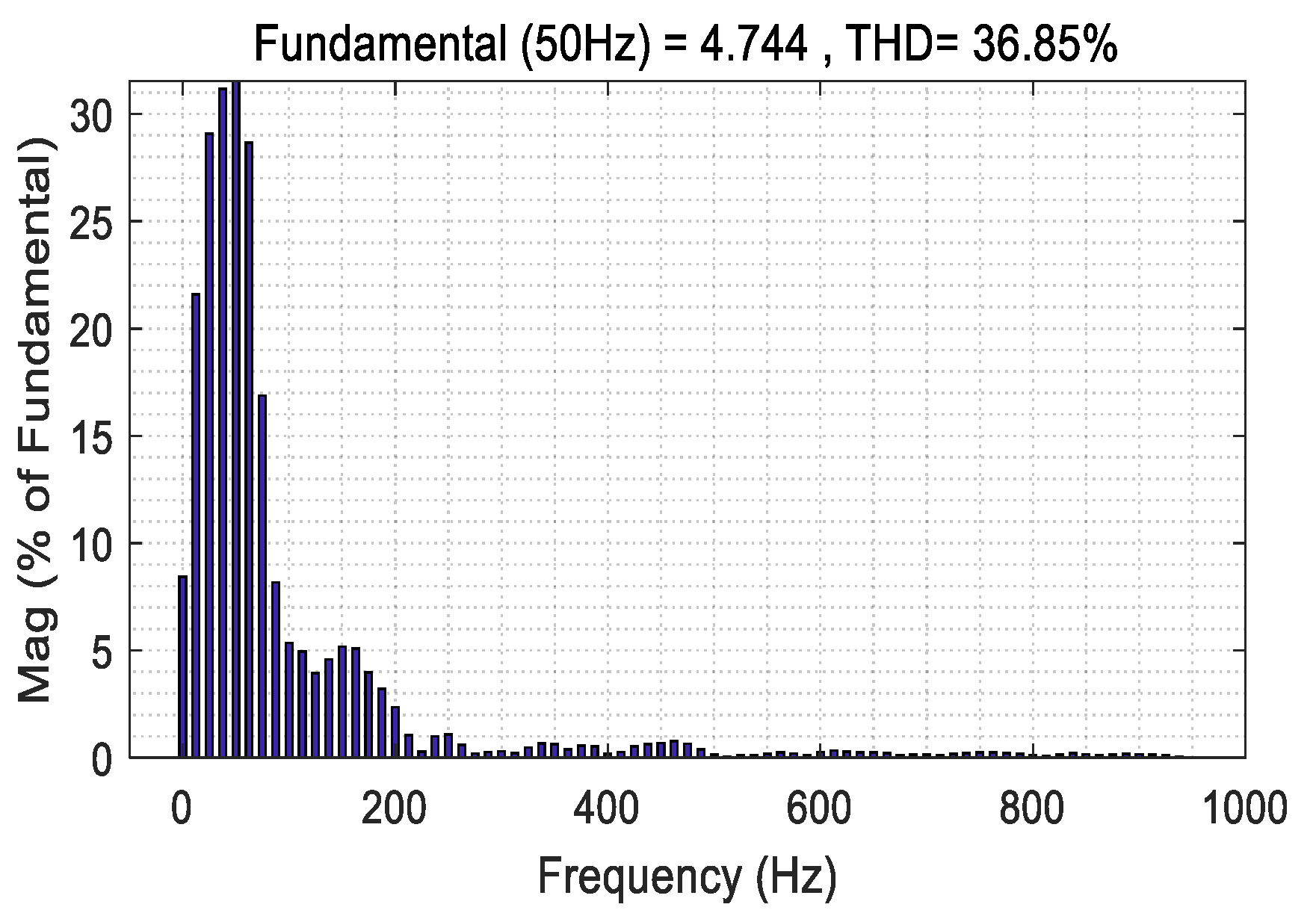
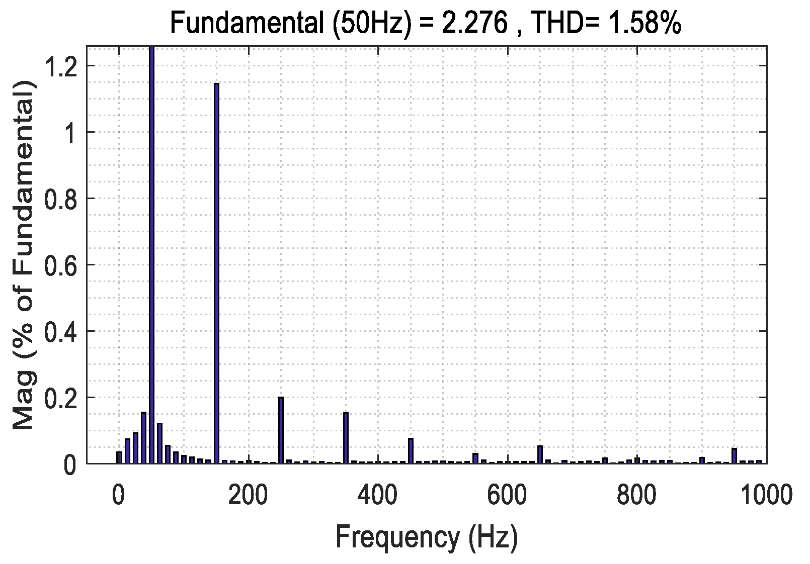
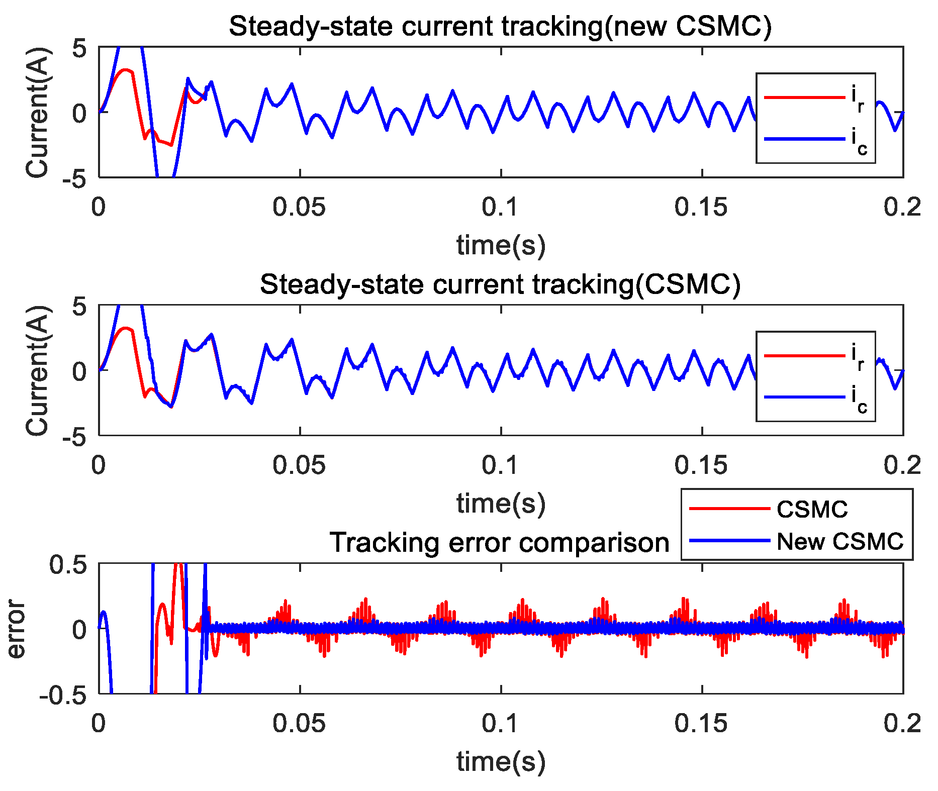
4.2. Steady-State Study
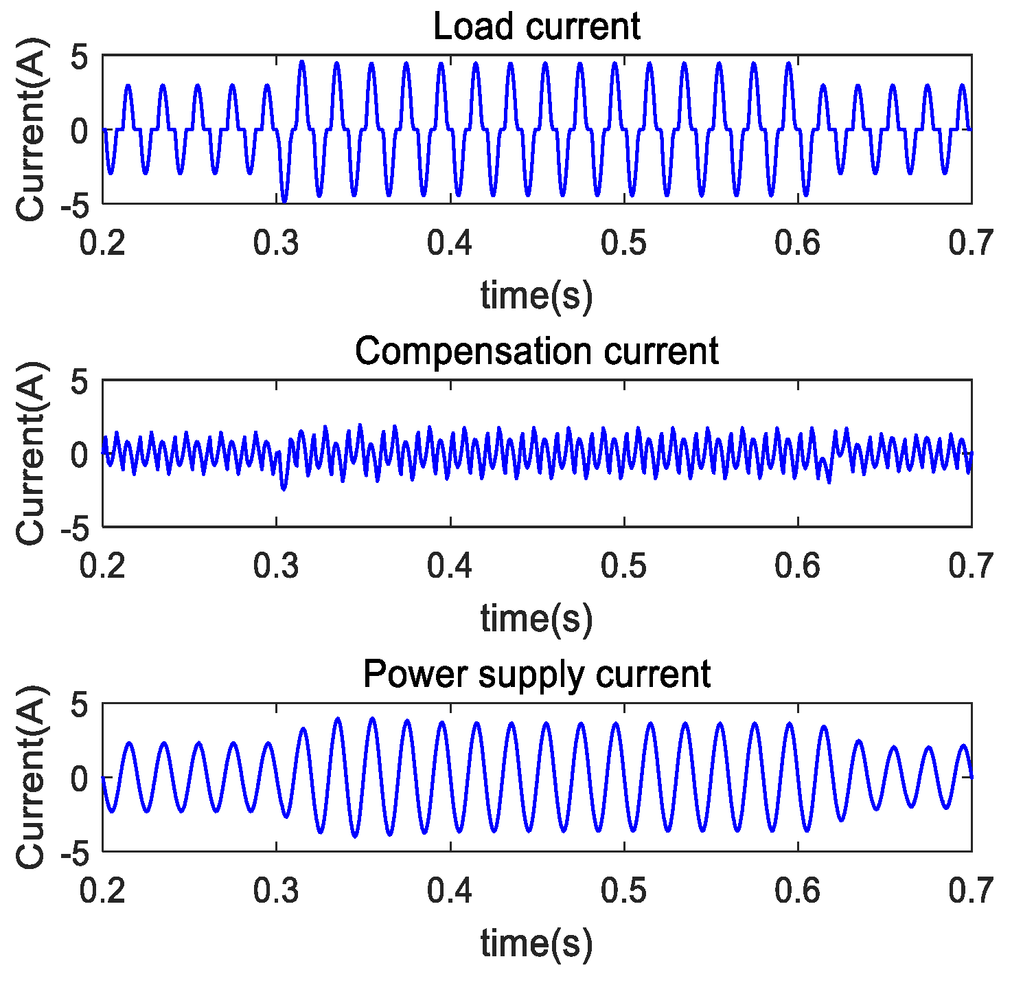
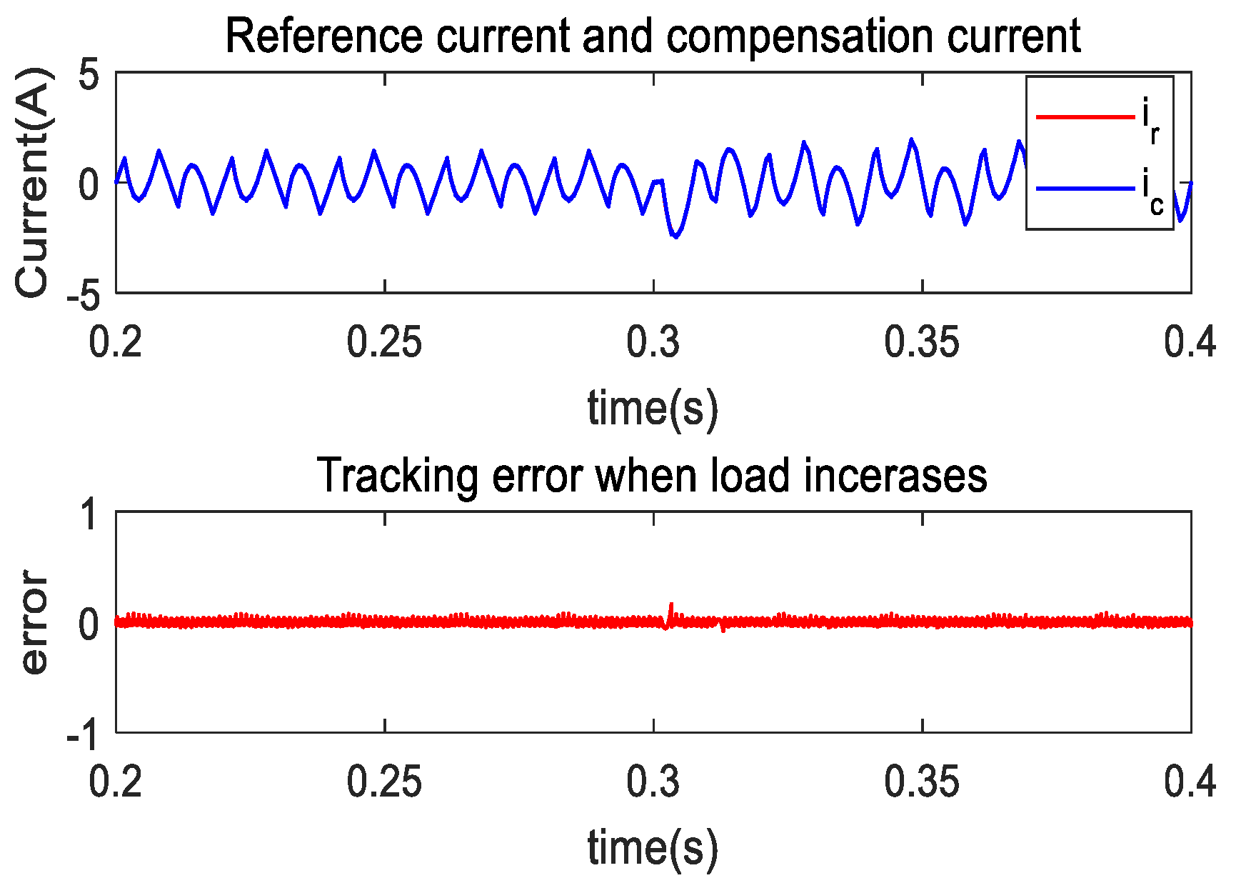
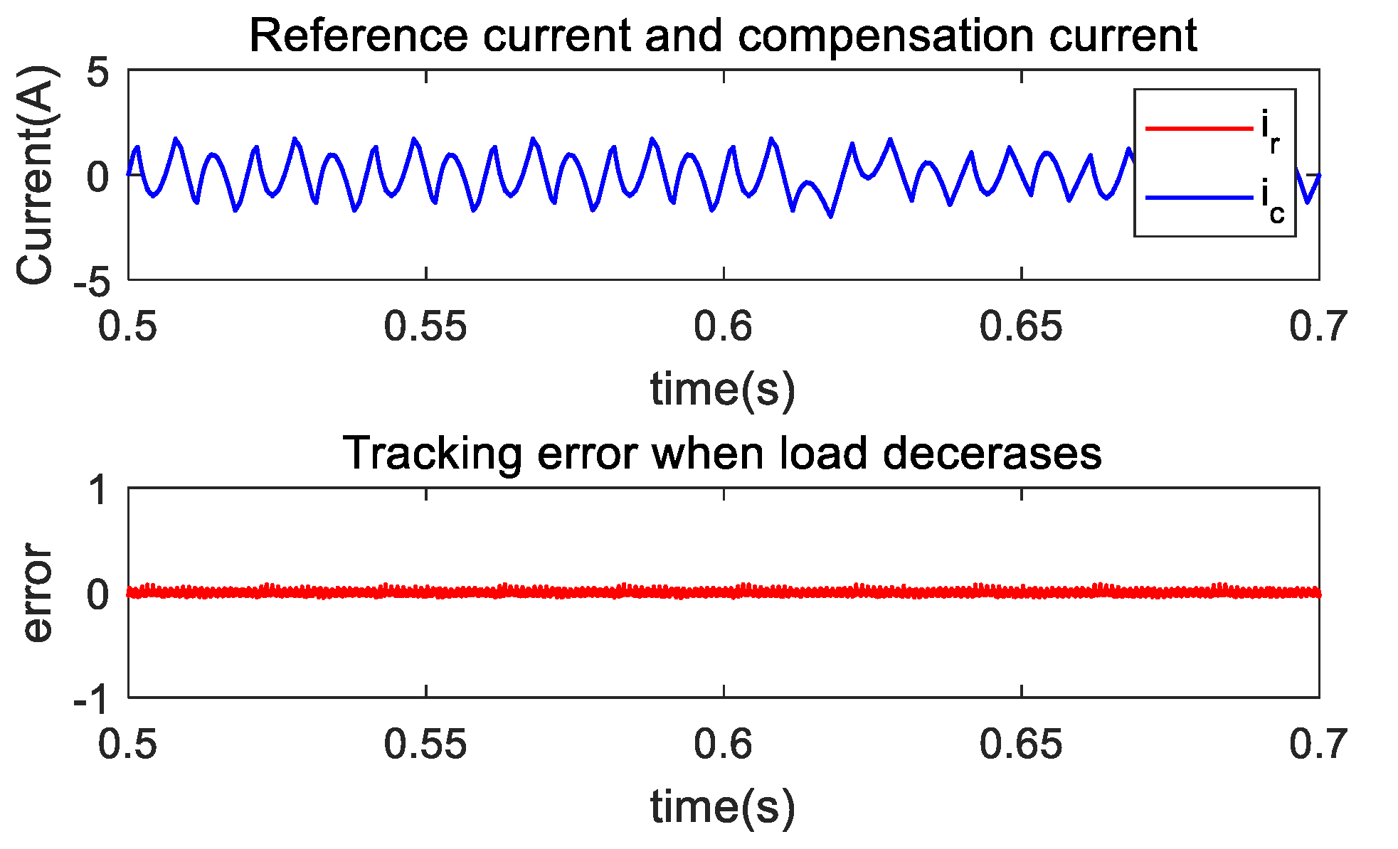
4.3. Dynamic Study
4.4. Comparison Study
5. Conclusions
Author Contributions
Funding
Data Availability Statement
Conflicts of Interest
Nomenclature
| ICSMC | Intelligent complementary sliding mode control |
| RBFNN | Radial basis function neural network |
| SECRBFNN | Self-evolving Chebyshev radial basis function neural network |
| CSMC | Complementary sliding mode control |
| ASMC | Adaptive sliding mode control |
| STSMC | Super-twisted sliding mode control |
| CN | Chebyshev network |
| NN | Neural network |
| FLNN | Functional link NN |
References
- Fuhui, G.; Pingli, L. Fast self-adapting high-order sliding mode control for a class of uncertain nonlinear systems. J. Syst. Eng. Electron. 2021, 32, 690–699. [Google Scholar] [CrossRef]
- Hong, Y.; Wang, J.; Cheng, D. Adaptive finite-time control of nonlinear systems with parametric uncertainty. IEEE Trans. Autom. Control 2006, 51, 858–862. [Google Scholar] [CrossRef]
- Lin, F.-J.; Chen, C.-I.; Xiao, G.-D.; Chen, P.-R. Voltage Stabilization Control for Microgrid With Asymmetric Membership Function-Based Wavelet Petri Fuzzy Neural Network. IEEE Trans. Smart Grid 2021, 12, 3731–3741. [Google Scholar] [CrossRef]
- Wang, A.; Liu, L.; Qiu, J.; Feng, G. Event-Triggered Robust Adaptive Fuzzy Control for a Class of Nonlinear Systems. IEEE Trans. Fuzzy Syst. 2019, 27, 1648–1658. [Google Scholar] [CrossRef]
- Zhang, R.-Y.; Wu, L.-B.; Zhao, N.-N.; Yan, Y. Adaptive Event-Triggered Fuzzy Tracking Control of Uncertain Stochastic Nonlinear Systems With Unmeasurable States. IEEE Trans. Fuzzy Syst. 2022, 30, 2183–2196. [Google Scholar] [CrossRef]
- Ang, K.H.; Chong, G.; Yun, L. PID control system analysis, design, and technology. IEEE Trans. Control. Syst. Technol. 2005, 13, 559–576. [Google Scholar] [CrossRef]
- Fei, J.; Chen, Y. Dynamic Terminal Sliding-Mode Control for Single-Phase Active Power Filter Using New Feedback Recurrent Neural Network. IEEE Trans. Power Electron. 2020, 35, 9904–9922. [Google Scholar] [CrossRef]
- Gwon, J.-S.; Lee, H.; Kim, S. Observer-Based FL-SMC Active Damping for Back-to-Back PWM Converter with LCL Grid Filter. Int. J. Fuzzy Log. Intell. Syst. 2015, 15, 200–207. [Google Scholar] [CrossRef]
- Fei, J.; Chen, Y. Fuzzy Double Hidden Layer Recurrent Neural Terminal Sliding Mode Control of Single-Phase Active Power Filter. IEEE Trans. Fuzzy Syst. 2021, 29, 3067–3081. [Google Scholar] [CrossRef]
- Lin, F.-J.; Chou, P.-H.; Chen, C.-S.; Lin, Y.-S. DSP-Based Cross-Coupled Synchronous Control for Dual Linear Motors via Intelligent Complementary Sliding Mode Control. IEEE Trans. Ind. Electron. 2012, 59, 1061–1073. [Google Scholar] [CrossRef]
- Liu, L.; Fei, J. Extended State Observer Based Interval Type-2 Fuzzy Neural Network Sliding Mode Control With Its Application in Active Power Filter. IEEE Trans. Power Electron. 2022, 37, 5138–5154. [Google Scholar] [CrossRef]
- Baek, J.; Jin, M.; Han, S. A New Adaptive Sliding-Mode Control Scheme for Application to Robot Manipulators. IEEE Trans. Ind. Electron. 2016, 63, 3628–3637. [Google Scholar] [CrossRef]
- Fei, J.; Liu, L. Real-Time Nonlinear Model Predictive Control of Active Power Filter Using Self-Feedback Recurrent Fuzzy Neural Network Estimator. IEEE Trans. Ind. Electron. 2022, 69, 8366–8376. [Google Scholar] [CrossRef]
- Balogoun, I.; Marx, S.; Liard, T.; Plestan, F. Super-Twisting Sliding Mode Control for the Stabilization of a Linear Hyperbolic System. IEEE Control. Syst. Lett. 2023, 7, 1–6. [Google Scholar] [CrossRef]
- Janardhanan, S.; Bandyopadhyay, B. Multirate Output Feedback Based Robust Quasi-Sliding Mode Control of Discrete-Time Systems. IEEE Trans. Autom. Control 2007, 52, 499–503. [Google Scholar] [CrossRef]
- Lin, F.-J.; Chen, S.-G.; Huang, M.-S.; Liang, C.-H.; Liao, C.-H. Adaptive Complementary Sliding Mode Control for Synchronous Reluctance Motor with Direct-Axis Current Control. IEEE Trans. Ind. Electron. 2022, 69, 141–150. [Google Scholar] [CrossRef]
- Lin, F.-J.; Hwang, J.-C.; Chou, P.-H.; Hung, Y.-C. FPGA-Based Intelligent-Complementary Sliding-Mode Control for PMLSM Servo-Drive System. IEEE Trans. Power Electron. 2010, 25, 2573–2587. [Google Scholar] [CrossRef]
- Fei, J.; Zhang, L.; Zhuo, J.; Fang, Y. Wavelet Fuzzy Neural Super-Twisting Sliding Mode Control of Active Power Filter. IEEE Trans. Fuzzy Syst. 2023, 3272028. [Google Scholar] [CrossRef]
- Zhang, L.; Fei, J. Intelligent Complementary Terminal Sliding Mode Using Multiloop Neural Network for Active Power Filter. IEEE Trans. Power Electron. 2023, 38, 9367–9383. [Google Scholar] [CrossRef]
- Fei, J.; Feng, Z. Fractional-Order Finite-Time Super-Twisting Sliding Mode Control of Micro Gyroscope Based on Double-Loop Fuzzy Neural Network. IEEE Trans. Syst. Man Cybern. Syst. 2021, 51, 7692–7706. [Google Scholar] [CrossRef]
- Lin, F.-J.; Chen, S.-G.; Hsu, C.-W. Intelligent Backstepping Control Using Recurrent Feature Selection Fuzzy Neural Network for Synchronous Reluctance Motor Position Servo Drive System. IEEE Trans. Fuzzy Syst. 2019, 27, 413–427. [Google Scholar] [CrossRef]
- Zhang, R.; Xu, B.; Shi, P. Output Feedback Control of Micromechanical Gyroscopes Using Neural Networks and Disturbance Observer. IEEE Trans. Neural Netw. Learn. Syst. 2022, 33, 962–972. [Google Scholar] [CrossRef]
- Fei, J.; Wang, H.; Fang, Y. Novel Neural Network Fractional-Order Sliding-Mode Control With Application to Active Power Filter. IEEE Trans. Syst. Man Cybern. Syst. 2022, 52, 3508–3518. [Google Scholar] [CrossRef]
- Fei, J.; Wang, Z.; Liang, X.; Feng, Z.; Xue, Y. Fractional Sliding-Mode Control for Microgyroscope Based on Multilayer Recurrent Fuzzy Neural Network. IEEE Trans. Fuzzy Syst. 2022, 30, 1712–1721. [Google Scholar] [CrossRef]
- Lai, W.; Peter, W.T.; Zhang, G.; Shi, T. Classification of gear faults using cumulants and the radial basis function network. Mech. Syst. Signal Process. 2004, 18, 381–389. [Google Scholar] [CrossRef]
- Zhang, L.; Li, K.; He, H.; Irwin, G.W. A new discrete-continuous algorithm for radial basis function networks construction. IEEE Trans. Neural Netw. Learn. Syst. 2013, 24, 1785–1798. [Google Scholar] [CrossRef]
- Stéphane, B.; Jin, H. Time delay compensation of digital control for DC switchmode power supplies using prediction techniques. IEEE Trans. Power Electron. 2000, 15, 835–842. [Google Scholar]
- Chen, C.H.; Lin, C.J.; Lin, C.T. A Functional-Link-Based Neurofuzzy Network for Nonlinear System Control. IEEE Trans. Fuzzy Syst. 2008, 16, 1362–1378. [Google Scholar] [CrossRef]
- Chen, S.-G.; Lin, F.-J.; Liang, C.-H.; Liao, C.-H. Intelligent Maximum Power Factor Searching Control Using Recurrent Chebyshev Fuzzy Neural Network Current Angle Controller for SynRM Drive System. IEEE Trans. Power Electron. 2021, 36, 3496–3511. [Google Scholar] [CrossRef]
- Fei, J.; Wang, Z.; Fang, Y. Self-Evolving Recurrent Chebyshev Fuzzy Neural Sliding Mode Control for Active Power Filter. IEEE Trans. Ind. Inform. 2023, 19, 2729–2739. [Google Scholar] [CrossRef]
- Chittora, P.; Singh, A.; Singh, M. Chebyshev Functional Expansion Based Artificial Neural Network Controller for Shunt Compensation. IEEE Trans. Ind. Inform. 2018, 14, 3792–3800. [Google Scholar] [CrossRef]
- Fei, J.; Wang, Z.; Pan, Q. Self-Constructing Fuzzy Neural Fractional-Order Sliding Mode Control of Active Power Filter. IEEE Trans. Neural Netw. Learn. Syst. 2022, 3169518. [Google Scholar] [CrossRef] [PubMed]
- Vo, A.T.; Truong, T.N.; Kang, H.-J. Fixed-Time RBFNN-Based Prescribed Performance Control for Robot Manipulators: Achieving Global Convergence and Control Performance Improvement. Mathematics 2023, 11, 2307. [Google Scholar] [CrossRef]
- Jäntschi, L.; Bolboacă, S.D.; Sestraş, R.E. Meta-heuristics on quantitative structure-activity relationships: Study on polychlorinated biphenyls. J. Mol. Model. 2010, 16, 77–86. [Google Scholar] [CrossRef] [PubMed]
- Wang, J.; Fang, Y.; Fei, J. Adaptive Super-Twisting Sliding Mode Control of Active Power Filter Using Interval Type-2-Fuzzy Neural Networks. Mathematics 2023, 11, 2785. [Google Scholar] [CrossRef]
- Zahraoui, Y.; Zaihidee, F.M.; Kermadi, M.; Mekhilef, S.; Mubin, M.; Tang, J.R.; Zaihidee, E.M. Fractional Order Sliding Mode Controller Based on Supervised Machine Learning Techniques for Speed Control of PMSM. Mathematics 2023, 11, 1457. [Google Scholar] [CrossRef]


| Parameters | Value |
|---|---|
| Grid voltage and frequency | |
| Nonlinear load at steady state | , , |
| Additional nonlinear loads in parallel | , , |
| Main circuit parameters of the SAPF | , , |
| Sampling period |
| Method | Parameters |
|---|---|
| CSMC | |
| New CSMC | |
| Voltage loop PI controller |
| Methods | RBFNN | DLRNN [12] | DHLRNN [7] | SECRBFNN |
|---|---|---|---|---|
| Time (s) | 25.194 | 49.737 | 75.641 | 42.562 |
| State\Strategy | THD of CSMC | THD of the New CSMC |
|---|---|---|
| Steady-state | 2.41% | 1.58% |
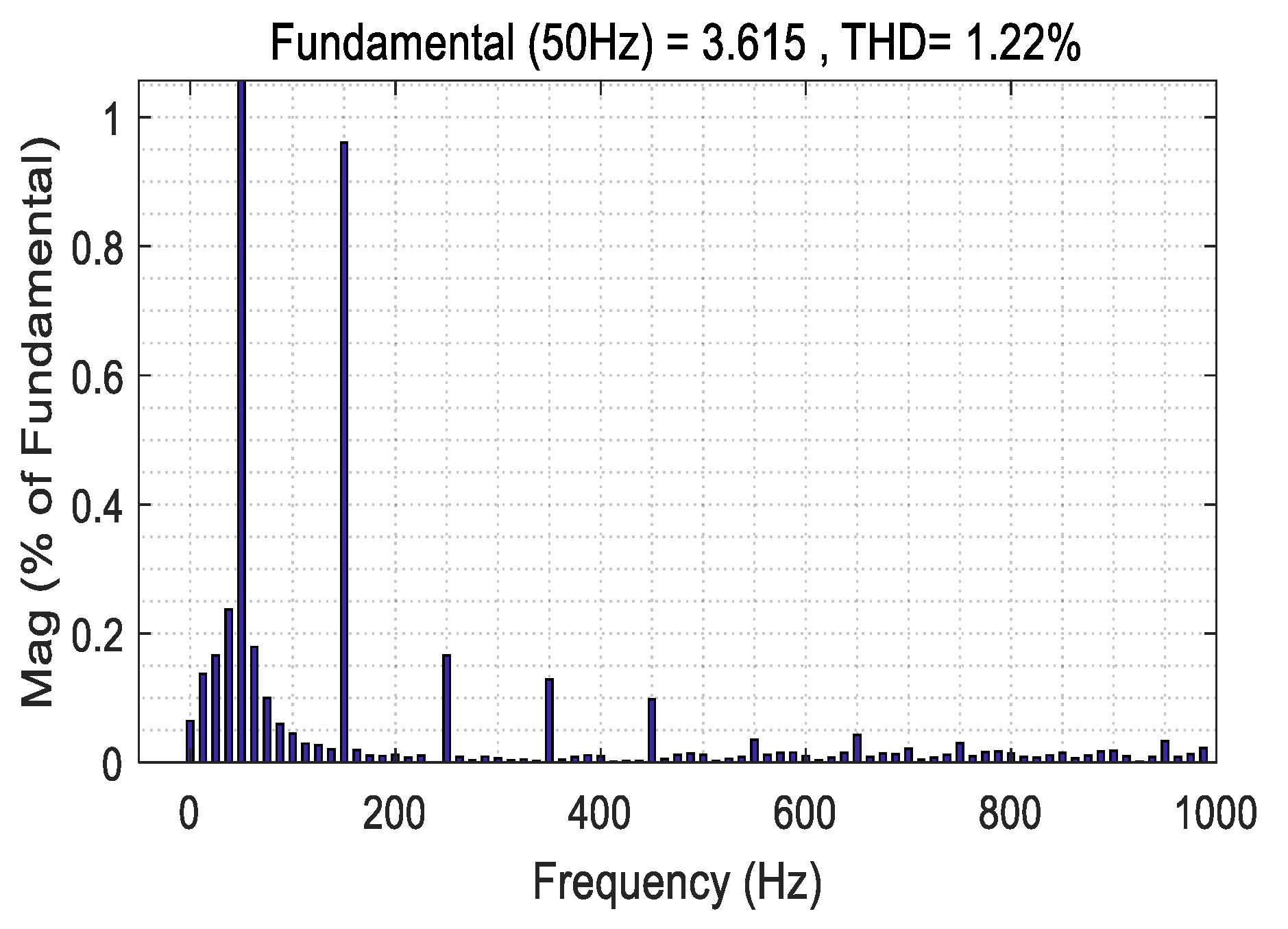
| After the load increases | 2.17% | 1.22% |
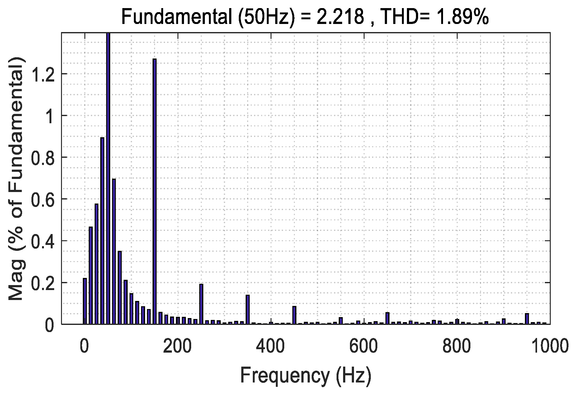
| After the load decreases | 2.64% | 1.89% |
Disclaimer/Publisher’s Note: The statements, opinions and data contained in all publications are solely those of the individual author(s) and contributor(s) and not of MDPI and/or the editor(s). MDPI and/or the editor(s) disclaim responsibility for any injury to people or property resulting from any ideas, methods, instructions or products referred to in the content. |
© 2023 by the authors. Licensee MDPI, Basel, Switzerland. This article is an open access article distributed under the terms and conditions of the Creative Commons Attribution (CC BY) license (https://creativecommons.org/licenses/by/4.0/).
Share and Cite
Zhang, L.; Li, X.; Fei, J. Self-Evolving Chebyshev Radial Basis Function Neural Complementary Sliding Mode Control. Mathematics 2023, 11, 3231. https://doi.org/10.3390/math11143231
Zhang L, Li X, Fei J. Self-Evolving Chebyshev Radial Basis Function Neural Complementary Sliding Mode Control. Mathematics. 2023; 11(14):3231. https://doi.org/10.3390/math11143231
Chicago/Turabian StyleZhang, Lei, Xiangguo Li, and Juntao Fei. 2023. "Self-Evolving Chebyshev Radial Basis Function Neural Complementary Sliding Mode Control" Mathematics 11, no. 14: 3231. https://doi.org/10.3390/math11143231
APA StyleZhang, L., Li, X., & Fei, J. (2023). Self-Evolving Chebyshev Radial Basis Function Neural Complementary Sliding Mode Control. Mathematics, 11(14), 3231. https://doi.org/10.3390/math11143231