Robust Closed–Open Loop Iterative Learning Control for MIMO Discrete-Time Linear Systems with Dual-Varying Dynamics and Nonrepetitive Uncertainties

Abstract

Iterative learning control (ILC) typically requires strict repeatability in initial states, trajectory length, external disturbances, and system dynamics. However, these assumptions are often difficult to fully satisfy in practical applications. While most existing studies have achieved limited progress in relaxing either one or two of these constraints simultaneously, this work aims to eliminate the restrictions imposed by all four strict repeatability conditions in ILC. For general finite-duration multi-input multi-output (MIMO) linear discrete-time systems subject to multiple non-repetitive uncertainties—including variations in initial states, external disturbances, trajectory lengths, and system dynamics—an innovative open-closed loop robust iterative learning control law is proposed. The feedforward component is used to make sure the tracking error converges as expected mathematically, while the feedback control part compensates for missing tracking data from previous iterations by utilizing real-time tracking information from the current iteration. The convergence analysis employs an input-to-state stability (ISS) theory for discrete parameterized systems. Detailed explanations are provided on adjusting key parameters to satisfy the derived convergence conditions, thereby ensuring that the anticipated tracking error will eventually settle into a compact neighborhood that meets the required standards for robustness and convergence speed. To thoroughly assess the viability of the proposed ILC framework, computer simulations effectively illustrate the strategy’s effectiveness. Further simulation on a real system, a piezoelectric motor system, verifies that the ILC tracking error converges to a small neighborhood in the sense of mathematical expectation. Extending the ILC to complex real-world applications provides new insights and approaches.

1. Introduction

As an efficient high-precision trajectory tracking method, ILC leverages the repetitive operation characteristics of controlled systems to dynamically optimize control input signals using historical iteration data [1,2,3]. The traditional ILC framework is based on strict repeatability assumptions, including invariant system dynamics, fixed trajectory lengths, iteration-invariant external disturbances, and precise initial state reproduction [4,5,6,7]. Under these assumptions, the ILC achieves zero-error tracking within finite iterations through a feedforward learning mechanism, with its efficacy validated in repetitive task scenarios such as rehabilitation robots [4], Euler–Bernoulli beam systems [5], and multi-agent collaborative systems [6,7].

However, the applicability of ILC is significantly constrained by pervasive non-repetitive factors in practical engineering systems. These challenges manifest as follows: (1) initial state deviations and non-repetitive external disturbances induced by environmental perturbations and equipment aging [8,9]; (2) iteration-varying trajectory lengths caused by evolving task requirements, e.g., early termination of iterations in gantry cranes under constraint activation [10] or stochastic fluctuations in train operation times [11]; (3) time-iteration two-dimensional varying system dynamics, such as the parameter drift in pharmaceutical crystallization processes [12] and position-dependent characteristics of permanent magnet synchronous motors [13]. While most studies focus on batch processes with time-invariant or time-varying models [14], few address systems with iteration-varying parameters [15]. Notably, the term “System with Dual-Varying Dynamics” in this study specifically refers to variations in the dual-dimensional time-iteration dynamic. Crucially, such dual-varying dynamics constitute one critical component within the broader framework of “multi-source non-repetitive uncertainties”.

Recent advances in non-repetitive ILC research have revealed several critical limitations. Parameter estimation-based ILC [16] addresses model variations but neglects trajectory length changes and disturbances. The robust model predictive ILC [17] handles disturbances and initial offsets but ignores model variations and trajectory length fluctuations. Machine earning-assisted ILC [18] integrates model variations and initial condition deviations but lacks disturbance suppression and trajectory length adaptability. Among the studies addressing model variations and disturbances [19,20,21,22,23], only four studies [21,23] considered initial state offsets, none of which tackled trajectory length variations. The sole work addressing trajectory length changes and model variations [24] failed to incorporate robustness against disturbances and deviations in the initial conditions. Thus, simultaneously relaxing the four repetitive constraints—constant model, fixed trajectory, iteration-invariant disturbances, and exact initial conditions—remains a critical theoretical challenge in ILC.

Modern engineering systems increasingly adopt MIMO architectures. For instance, in the field of wireless communications, MIMO systems employ multiple transmitting and receiving antennas to exploit spatial diversity [25,26]. Beyond telecommunications, MIMO principles have been extended to data-driven [27], industrial printing [28], and smart robotic [29] technologies, where the coordinated control of multiple actuators/sensors enables robustness against disturbances and uncertainties. However, the advantages of MIMO architectures are accompanied by inherent challenges, including channel-state estimation, interference alignment, and computational complexity in high-dimensional configurations.

To bridge the above studies, this paper proposes a novel open–closed loop composite robust ILC framework for MIMO linear discrete systems with multi-source non-repetitive uncertainties, with the following key innovations:

• The feedforward component ensures the convergence of tracking errors in the mathematical expectation, while the feedback controller compensates for missing tracking data from prior iterations using real-time tracking information.
• Comprehensive Handling of Multi-Source Non-Repetitive Uncertainties:
  • Time-iteration dual-dimensional system dynamics variations.
  • Iteration-varying trajectory lengths caused by stochastic task requirements.
  • Non-repetitive external disturbances.
  • Initial state deviations across iterations.
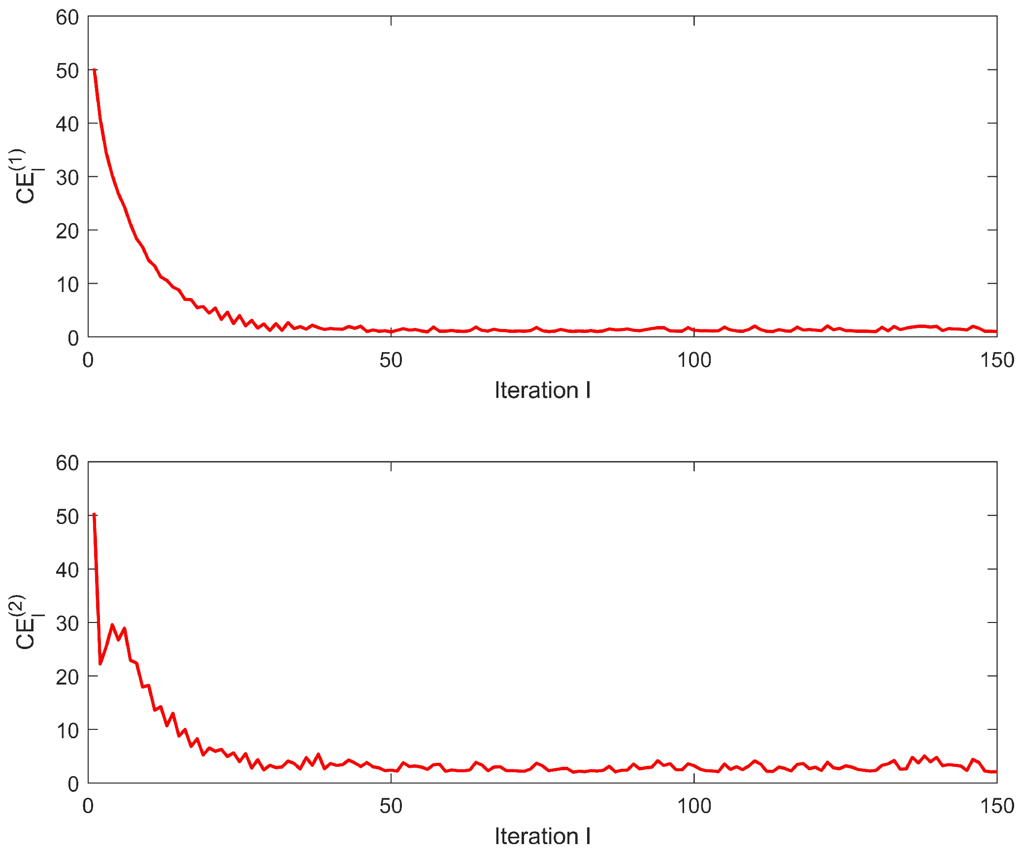
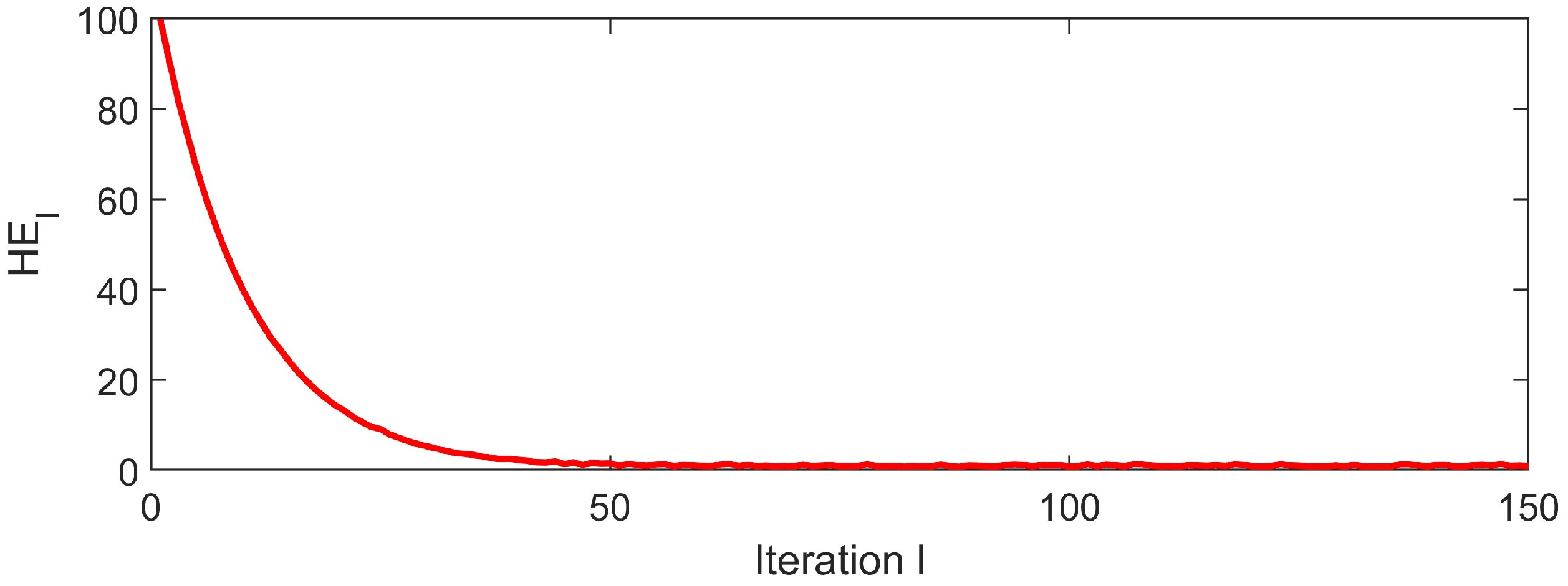
• Quantitative mappings between controller parameters and convergence rate/robustness metrics are established to guide algorithmic tuning. Experimental simulations on a piezoelectric motor system demonstrate ILC tracking error convergence to an ε-neighborhood in expectation. The feasibility of the proposed iterative learning control architecture was further confirmed through rigorous numerical simulation experiments, which provided quantitative performance validation for the transition of the open–closed loop iterative learning control law from theoretical formulation to practical operational environments.

The framework of this technical note is outlined in the following manner: Section 2 provides the problem statement, followed by Section 3, which presents the open–closed loop ILC system and associated robustness and convergence analysis. A relevant example is presented in Section 4, while Section 5 offers the concluding thoughts of this study.

Notations: The paper uses $\Vert ·\Vert$ denote the compatible norm of vector and matrix. Mathematical expectation of a stochastic variable is denoted by $E\left\{·\right\}$.

2. Problem Formulation

2.1. Dynamics Description

Think of this discrete-time, non-repetitive linear MIMO system where the tracking lengths and disturbances are iteratively variable:

$$\left\{\begin{array}{c}{x}_l\left(t+1\right)=A_l\left(t\right)x_l\left(t\right)+B_l\left(t\right)u_l\left(t\right)+w_l\left(t\right)\\ y_l\left(t\right)=C_l\left(t\right)x_l\left(t\right)+v_l\left(t\right)\end{array}\right.,$$

(1)

where the iteration index is represented by $l\in \left\{0,1,\cdots \right\}$, and the discrete time index is represented by $t\in \left\{0,1,\cdots ,N_l\right\}$. $N_l$ represents the system’s trail length at the $lth$ iteration, which varies unpredictably from one iteration to the next and is unknown. Meanwhile $x_l\left(t\right)\in R^n$, $u_l\left(t\right)\in R^m$ and $y_l\left(t\right)\in R^p$ are the state, input, and output, respectively. ${\omega }_l\left(t\right)\in R^n$ and ${\upsilon }_l\left(t\right)\in R^p$ are the state disturbances and output disturbances, respectively; $A_l\left(t\right)\in R^{n\times n}$, $B_l\left(t\right)\in R^{n\times m}$, $C_l\left(t\right)\in R^{p\times n}$ are the system matrices. $A_l\left(t\right)\in R^{n\times n}$ is the state transition matrix that characterizes the natural evolution of the system’s internal states. $B_l\left(t\right)\in R^{n\times m}$ is the input control matrix, describing how external control inputs drive the system states. $C_l\left(t\right)\in R^{p\times n}$ is the observation output matrix that maps internal states to measurable outputs. Through the expression of the system matrix, we can see that the non-repetitive dynamical system varies with time and the number of iterations, i.e., dual-varying dynamics.

The reference trajectory $r\left(t\right)\in R^p$ for $t\in \left\{0,1,\cdots ,N_d\right\}$. Considering any achievable trajectory $r\left(t\right)$, there is a one-of-a-kind control input $u_d\left(t\right)\in R^m$ for $t\in \left\{0,1,\cdots ,N_d\right\}$ so the following applies:

$$\left\{\begin{array}{l}{x}_d\left(t+1\right)=A\left(t\right)x_d\left(t\right)+B\left(t\right)u_d\left(t\right)\hfill \\ r\left(t\right)=C\left(t\right)x_d\left(t\right)\hfill \end{array}\right.$$

(2)

where $x_d\left(t\right)$ and $N_d$ are the target state and target operation length, respectively.

Following this definition, the non-repetitive linear discrete-time MIMO system’s ILC tracking error is $e_l\left(t\right)=r\left(t\right)-y_l\left(t\right)$, $t\in \left\{0,1,\cdots ,\min \left\{N_l+1,N_d+1\right\}\right\}$.

The non-repetitive MIMO system (1) is subject to the following assumptions.

A1: 

Boundedness: Assume that, for all $l\in \left\{0,1,\cdots \right\}$ and $t\in \left\{0,1,\cdots ,N_d\right\}$

$$\begin{array}{cccc}\Vert A_l\left(t\right)\Vert \le {\beta }_A\hfill & \Vert B_l\left(t\right)\Vert \le {\beta }_B\hfill & \Vert C_l\left(t\right)\Vert \le {\beta }_C\hfill & \Vert u_d\left(t\right)\Vert \le {\beta }_{u_d}\hfill \\ \Vert A\left(t\right)\Vert \le {\beta }_{\overline{A}}\hfill & \Vert B\left(t\right)\Vert \le {\beta }_{\overline{B}}\hfill & \Vert C\left(t\right)\Vert \le {\beta }_{\overline{C}}\hfill & \Vert x_d\left(t\right)\Vert \le {\beta }_{x_d}\hfill \\ \Vert {\omega }_l\left(t\right)\Vert \le {\beta }_{\omega }\hfill & \Vert {\upsilon }_l\left(t\right)\Vert \le {\beta }_{\upsilon }\hfill \end{array}$$

(3)

where ${\beta }_A\ge 0$, ${\beta }_B\ge 0$, ${\beta }_C\ge 0$,${\beta }_{u_d}\ge 0$,${\beta }_{\overline{A}}\ge 0$,${\beta }_{\overline{B}}\ge 0$,${\beta }_{\overline{C}}\ge 0$,${\beta }_{x_d}\ge 0$, ${\beta }_{\omega }\ge 0$, and ${\beta }_{\upsilon }\ge 0$ are some finite bounds.

A2: 

Convergence in Iteration: Assume that, for all $l\in \left\{0,1,\cdots \right\}$

$$\begin{array}{ccc}\underset{l\to \infty }{\lim }{A}_l(t)=A(t),& \underset{l\to \infty }{\lim }{B}_l(t)=B(t),& \underset{l\to \infty }{\lim }{C}_l(t)=C(t)\end{array}$$

(4)

for some iteration-invariant matrices $A\left(t\right)$, $B\left(t\right)$, and $C\left(t\right)$.

A3: 

Expectation of State: The iterative initial state $x_l\left(0\right)$ is unpredictably variable, but its mathematical expectation meets $E\left\{x_l\left(0\right)\right\}=x_d\left(0\right)$.

Definition 1.

Two vectors $\Xi ={\left[{\Xi }^{\left(1\right)},{\Xi }^{\left(2\right)},\cdots ,{\Xi }^{\left(\eta \right)}\right]}^T\in R^{\eta }$ and ${\rm Y}={\left[{{\rm Y}}^{\left(1\right)}{{\rm Y}}^{\left(2\right)}\cdots {{\rm Y}}^{\left(\eta \right)}\right]}^T\in R^{\eta }$ are defined to satisfy the inequality $\Xi \le {\rm Y}$ if and only if the relation ${\Xi }^{\left(j\right)}\le {{\rm Y}}^{\left(j\right)}$ holds for every element $j\in \left\{1,2,\cdots ,\eta \right\}$.

Remark 1.

Unlike general ILC’s identical-initial condition requirement $x_l\left(0\right)=x_d\left(0\right)$, assumption (A3) relaxes it, allowing $x_l\left(0\right)$ to be a random variable with fixed expectation $x_d\left(0\right)$.

For system (1) with iteration-varying trajectory lengths and given assumptions, the objective of ILC is to design a control input sequence $\left\{u_l\left(t\right)\right\}$ that guarantees bounded tracking errors and minimizes their magnitude under disturbances.

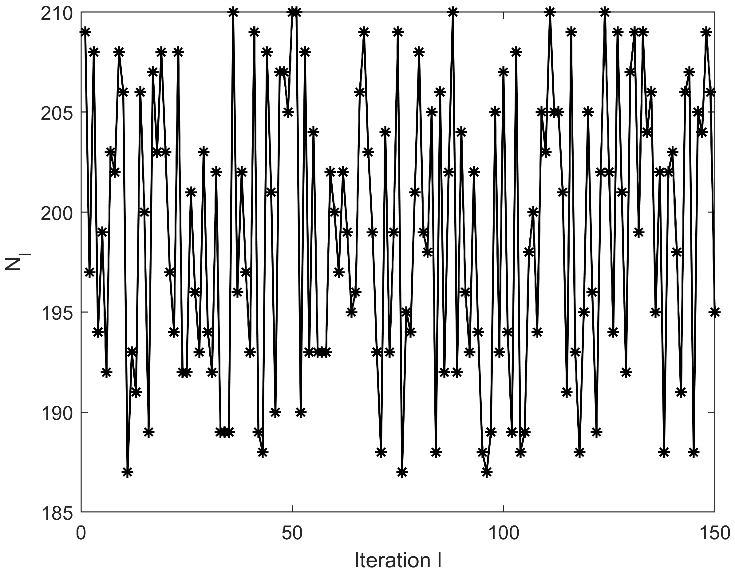
2.2. Varying Iteration Lengths

When it comes to applications, the desired operation length $N_d$ and the actual operation length $N_l$ could differ. The duration of different iterative stages is typically non-uniform, as exemplified by the premature termination of iterations in gantry crane operations due to activated constraints [10] or stochastic fluctuations in train travel times [11]. No prior knowledge of $\underset{\_}{N}$ or $\overline{N}$ is required for this article; we will instead assume that they are the minimum and maximum operation lengths, respectively. In other words, the design of the ILC scheme does not incorporate the particular details of $\underset{\_}{N}$ and $\overline{N}$. $N_l\left(N\le N_l\le \overline{N}\right)$ is the unknown and randomly changeable actual trail length of the system at the $lth$ iteration.

For non-repetitive linear discrete-time MIMO systems (1) with trajectory lengths that vary with iteration, we formulate ${\xi }_l\left(t\right)$$\left(t\in \left\{0,1,\cdots ,N_d\right\}\right)$ as a Bernoulli-distributed stochastic variable with binary values $\left\{0,1\right\}$ in order to solve the ILC issue. In this case, ${\xi }_l\left(t\right)=1$ indicates that the control input of system (1) continues until time point $t$ in the $lth$ iteration, with a probability function associated with $p\left(t\right)\left(0<p\left(t\right)\le 1\right)$. ${\xi }_l\left(t\right)=0$ means the event where the control input fails to persist until $t$, occurring with probability $\left[1-p\left(t\right)\right]$. Obviously, the expectation of ${\xi }_l\left(t\right)$ is $E\left\{{\xi }_l\left(t\right)\right\}=1·p\left(t\right)+0·\left(1-p\left(t\right)\right)=$ $p\left(t\right)$.

To account for the iteration-varying trajectory lengths in system (1), the corrected tracking error is defined as follows:

$${\tilde{e}}_l\left(t\right)={\xi }_l\left(t\right)·e_l(t)\mathrm{t}\in \{0,1,\cdots ,N_d\}$$

(5)

Given the description of Bernoulli-distributed stochastic variable ${\xi }_l\left(t\right)$, (5) can be rewritten as for $N_l<N_d$,

$${\tilde{e}}_l(t)=\left\{\begin{array}{ll}{e}_l(t),\hfill & t\in \left\{0,1,\cdots ,N_l\right\}\hfill \\ 0,\hfill & t\in \left\{N_l+1,\cdots ,N_d\right\}\hfill \end{array}\right.$$

(6)

and for $N_l\ge N_d$,

$${\tilde{e}}_l\left(t\right)=e_l\left(t\right),t\in \left\{0,1,\cdots N_d\right\}.$$

(7)

Based on Equation (5) and $E\left\{{\xi }_l\left(t\right)\right\}=p\left(t\right)$, we obtain the following:

$$E\left\{{\tilde{e}}_l\left(t\right)\right\}=p\left(t\right)E\left\{e_l\left(t\right)\right\}.$$

(8)

Lemma 1

([30]). Let $\left\{{\alpha }_g\right\}$ with $g\ge N+1$ be a real sequence defined as ${\alpha }_g\le \zeta ·{\alpha }_{g-1}+\overline{b}$ , where $\overline{b}$ is a bounded value. If $\zeta$ satisfies $\zeta <1$, then we can obtain $\underset{g\to \infty }{\lim }sup{\alpha }_g\le {\displaystyle \frac{\overline{b}}{1-\zeta }}$.

We exclude the proofs of Lemma 1 here because of the page limitation, although they are derived by following similar processes as stability proofs of discrete linear time-varying systems (see, e.g., [30]).

3. Open–Closed Loop Designs with Robustness and Convergence Analysis

An open–closed loop law for $t\in \left\{0,1,\cdots ,N_d\right\}$ with adjusted tracking error is proposed for robustness and convergence analysis for the system (1) under assumptions (A1)–(A3), as shown below.

$$u_{l+1}\left(t\right)=u_{f,l+1}\left(t\right)+u_{b,l+1}\left(t\right)$$

(9)

$$u_{f,l+1}\left(t\right)=u_l\left(t\right)+P{\tilde{e}}_l\left(t+1\right)$$

(10)

$$u_{b,l+1}\left(t\right)=T{\tilde{e}}_{l+1}\left(t\right)$$

(11)

where $u_{f,l+1}\left(t\right)$ represents the ILC component with feed-forward control gain matrix $P\in R^{m\times p}$ and $u_{b,l+1}\left(t\right)$ symbolizes the feedback control component with feedback control gain matrix $T\in R^{m\times p}$.

Theorem 1.

Under assumptions (A1)–(A3), for the dual-varying non-repetitive linear discrete-time MIMO system (1) with iteratively variable trail lengths, initial condition deviations, and disturbances, the open–closed loop ILC law (9)–(11) is used. If the control gain $P\in R^{m\times p}$ is selected to make the following:

$$\Vert \left[I-p\left(t+1\right)P{C}_l\left(t+1\right)B_l\left(t\right)\right]\Vert \le \epsilon <1,$$

(12)

where $0\le t\le N_d$ . We conclude that $\underset{l\to +\infty }{\lim }sup\Vert E\left\{e_l\left(t\right)\right\}\Vert$ is bounded such that $\underset{l\to +\infty }{\lim }sup\Vert E\left\{e_l\left(t\right)\right\}\Vert \le {\beta }_e$, where ${\beta }_e$ is finite bound. Furthermore, if we additionally have the assumption (A2) in the absence of disturbances, we can conclude that $\underset{l\to +\infty }{\lim }sup\Vert E\left\{e_l\left(t\right)\right\}\Vert =0$ i.e., ${\beta }_e=0$ for $t\in \left\{0,1,\cdots ,N_d+1\right\}$.

Proof. 

Denote $\delta u_{f,l}\left(t\right)=u_d-u_{f,l}\left(t\right)$ and $\delta u_l\left(t\right)=u_d-u_l\left(t\right)$. Deducting $u_d\left(t\right)$ from both sides of (10), it produces the following:

$$\delta u_{f,l+1}\left(t\right)=\delta u_l\left(t\right)-P{\tilde{e}}_l(t+1)$$

(13)

Taking $E\left\{·\right\}$ on both sides of (13) and considering (8), we have

$$E\left\{\delta u_{f,l+1}\left(t\right)\right\}=E\left\{\delta u_l\left(t\right)\right\}-P·E\left\{{\tilde{e}}_l(t+1)\right\}=E\left\{\delta u_l\left(t\right)\right\}-p(t+1)·P·E\left\{e_l(t+1)\right\}$$

(14)

Let $\delta x_l\left(t\right)=x_d\left(t\right)-x_l\left(t\right)$. Based on (1) and (2), and by simplifying and combining $E\left\{\delta u_l\left(t\right)\right\}$, (14) becomes the following:

$$\begin{array}{ll}E\left\{\delta u_{f,l+1}\left(t\right)\right\}\hfill & =E\left\{\delta u_l\left(t\right)\right\}-p(t+1)PE\left\{C\left(t+1\right)x_d\left(t+1\right)-C_l\left(t+1\right)x_l\left(t+1\right)-{\upsilon }_l\left(t+1\right)\right\}\hfill \\ & =E\left\{\delta u_l\left(t\right)\right\}-p(t+1)PE\left\{C\left(t+1\right)\left[A\left(t\right)x_d\left(t\right)+B\left(t\right)u_d\left(t\right)\right]\right.\hfill \\ & \hspace{1em}\left.-C_l\left(t+1\right)\left[A_l\left(t\right)x_l\left(t\right)+B_l\left(t\right)u_l\left(t\right)+w_l\left(t\right)\right]-{\upsilon }_l\left(t+1\right)\right\}\hfill \\ & =E\left\{\delta u_l\left(t\right)\right\}-p(t+1)PE\left\{C_l\left(t+1\right)A_l\left(t\right)\delta x_l\left(t\right)+C_l\left(t+1\right)B_l\left(t\right)\delta u_l\left(t\right)\right.\hfill \\ & \hspace{1em}\left.-C_l\left(t+1\right){\omega }_l\left(t\right)-{\upsilon }_l\left(t+1\right)\right\}-p(t+1)P\left[C\left(t+1\right)A\left(t\right)-C_l\left(t+1\right)A_l\left(t\right)\right]x_d\left(t\right)\hfill \\ & \hspace{1em}-p(t+1)P\left[C\left(t+1\right)B\left(t\right)-C_l\left(t+1\right)B_l\left(t\right)\right]u_d\left(t\right)\hfill \\ & =\left[I-p\left(t+1\right)P{C}_l\left(t+1\right)B_l\left(t\right)\right]E\left\{\delta u_l\left(t\right)\right\}\hfill \\ & \hspace{1em}-p(t+1)PE\left\{C_l\left(t+1\right)A_l\left(t\right)\delta x_l\left(t\right)-C_l\left(t+1\right){\omega }_l\left(t\right)-{\upsilon }_l\left(t+1\right)\right\}\hfill \\ & \hspace{1em}-p(t+1)P\left[C\left(t+1\right)A\left(t\right)-C_l\left(t+1\right)A_l\left(t\right)\right]x_d\left(t\right)\hfill \\ & \hspace{1em}-p(t+1)P\left[C\left(t+1\right)B\left(t\right)-C_l\left(t+1\right)B_l\left(t\right)\right]u_d\left(t\right)\hfill \end{array}$$

(15)

From (9) and (11), it follows

$$\begin{array}{cc}\hfill \delta u_l\left(t\right)& \hfill =\delta u_{f,l}\left(t\right)-u_{b,l}\left(t\right)\\ & \hfill =\delta u_{f,l}\left(t\right)-{T\tilde{e}}_l\left(t\right)\end{array}$$

(16)

Taking $E\left\{·\right\}$ on both sides of (16) and noticing (8), yield

$$E\left\{\delta u_l\left(t\right)\right\}=E\left\{\delta u_{f,l}\left(t\right)\right\}-p\left(t\right)T·E\left\{e_l\left(t\right)\right\}$$

(17)

Substituting (17) into (15) derives that

$$\begin{array}{cc}E\left\{\delta u_{f,l+1}\left(t\right)\right\}\hfill & =\left[I-p\left(t+1\right)P{C}_l\left(t+1\right)B_l\left(t\right)\right]E\left\{\delta u_{f,l}\left(t\right)\right\}-p\left(t\right)T\left[I-p\left(t+1\right)P{C}_l\left(t+1\right)B_l\left(t\right)\right]E\left\{e_l\left(t\right)\right\}\hfill \\ & \hspace{1em}-p(t+1)PE\left\{C_l\left(t+1\right)A_l\left(t\right)\delta x_l\left(t\right)-C_l\left(t+1\right){\omega }_l\left(t\right)-{\upsilon }_l\left(t+1\right)\right\}\hfill \\ & \hspace{1em}-p(t+1)P\left[C\left(t+1\right)A\left(t\right)-C_l\left(t+1\right)A_l\left(t\right)\right]x_d\left(t\right)\hfill \\ & \hspace{1em}-p(t+1)P\left[C\left(t+1\right)B\left(t\right)-C_l\left(t+1\right)B_l\left(t\right)\right]u_d\left(t\right)\hfill \end{array}$$

(18)

Taking norm $\Vert ·\Vert$ on both sides of (18), there is

$$\begin{array}{cc}\Vert E\left\{\delta u_{f,l+1}\left(t\right)\right\}\Vert \hfill & \le \Vert I-p\left(t+1\right)P{C}_l\left(t+1\right)B_l\left(t\right)\Vert ·\Vert E\left\{\delta u_{f,l}\left(t\right)\right\}\Vert \hfill \\ & +p\left(t\right)\Vert T\Vert \Vert I-p\left(t+1\right)P{C}_l\left(t+1\right)B_l\left(t\right)\Vert \Vert E\left\{e_l\left(t\right)\right\}\Vert \hfill \\ & +p(t+1)\Vert P\Vert ·\Vert C_l\left(t+1\right)A_l\left(t\right)\Vert \Vert E\left\{\delta x_l\left(t\right)\right\}\Vert \hfill \\ & +p(t+1)\Vert P\Vert \Vert C_l\left(t+1\right)\Vert ·\Vert E\left\{{\omega }_l\left(t\right)\right\}\Vert +p(t+1)\Vert P\Vert \Vert E\left\{{\upsilon }_l\left(t+1\right)\right\}\Vert \hfill \\ & +p(t+1)\Vert P\Vert \Vert \left[C\left(t+1\right)A\left(t\right)-C_l\left(t+1\right)A_l\left(t\right)\right]x_d\left(t\right)\Vert \hfill \\ & +p(t+1)\Vert P\Vert \Vert \left[C\left(t+1\right)B\left(t\right)-C_l\left(t+1\right)B_l\left(t\right)\right]u_d\left(t\right)\Vert \hfill \\ & \le \epsilon \Vert E\left\{\delta u_{f,l}\left(t\right)\right\}\Vert +z_1\left\{\Vert E\left\{\delta x_l\left(t\right)\right\}\Vert +\Vert E\left\{e_l\left(t\right)\right\}\Vert \right\}+z_2\hfill \end{array}$$

(19)

where $z_1=\max \left\{\overline{p}·\Vert T\Vert \epsilon ,\overline{p}\Vert P\Vert {\beta }_C{\beta }_A\right\}$ and $z_2=\overline{p}\Vert P\Vert {\beta }_C{\beta }_{\omega }+\overline{p}\Vert P\Vert {\beta }_{\upsilon }+\overline{p}\Vert P\Vert \left({\beta }_{\overline{C}}{\beta }_{\overline{A}}\right.$$-{\beta }_C$$\left.{\beta }_A\right){\beta }_{x_d}+\overline{p}\Vert P\Vert \left({\beta }_{\overline{C}}{\beta }_{\overline{B}}-{\beta }_C{\beta }_B\right){\beta }_{u_d}$ with $\Vert \left[I-p\left(t+1\right)P{C}_l\left(t+1\right)B_l\left(t\right)\right]\Vert \le \epsilon <1$ by condition (9) and $\overline{p}=\underset{i\in \left\{0,\cdots ,N_d+1\right\}}{\max }p\left(i\right)$.

On the other hand, according (1), (2), and by substituting (17), there are

$$\begin{array}{cc}E\left\{e_l\left(t\right)\right\}\hfill & =E\left\{r\left(t\right)-y_l\left(t\right)\right\}=E\left\{C\left(t\right)x_d\left(t\right)-C_l\left(t\right)x_l\left(t\right)-{\upsilon }_l\left(t\right)\right\}\hfill \\ & =E\left\{C\left(t\right)\left[A\left(t-1\right)x_d(t-1)+B(t-1)u_d(t-1)\right]\right.\hfill \\ & \hspace{1em}-C_l\left(t\right)\left[A_l(t-1)x_l(t-1)+B_l(t-1)u_l(t-1)+{\omega }_l(t-1)\right]\left.-{\upsilon }_l\left(t\right)\right\}\hfill \\ & =C_l\left(t\right)A_l(t-1)E\left\{\delta x_l(t-1)\right\}\hfill \\ & \hspace{1em}+C_l\left(t\right)B_l(t-1)E\left\{\delta u_l(t-1)\right\}\hfill \\ & \hspace{1em}+\left[C\left(t\right)A(t-1)-C_l\left(t\right)A_l(t-1)\right]x_d(t-1)\hfill \\ & \hspace{1em}+\left[\left(C\left(t\right)B(t-1)-C_l\left(t\right)B_l(t-1)\right]u_d(t-1)\right.\hfill \\ & \hspace{1em}-C_l\left(t\right)E\left\{{\omega }_l(t-1)\right\}-E\left\{{\upsilon }_l\left(t\right)\right\}\hfill \\ & =C_l\left(t\right)A_l(t-1)E\left\{\delta x_l(t-1)\right\}\hfill \\ & \hspace{1em}+C_l\left(t\right)B_l(t-1)E\left\{\delta u_{f,l}(t-1)\right\}-p\left(t\right)T·C_l\left(t\right)B_l(t-1)E\left\{e_l(t-1)\right\}\hfill \\ & \hspace{1em}+\left[C\left(t\right)A(t-1)-C_l\left(t\right)A_l(t-1)\right]x_d(t-1)\hfill \\ & \hspace{1em}+\left[\left(C\left(t\right)B(t-1)-C_l\left(t\right)B_l(t-1)\right]u_d(t-1)\right.\hfill \\ & \hspace{1em}-C_l\left(t\right)E\left\{{\omega }_l(t-1)\right\}-E\left\{{\upsilon }_l\left(t\right)\right\}\hfill \end{array}$$

(20)

and

$$\begin{array}{cc}E\left\{\delta x_l\left(t\right)\right\}\hfill & =E\left\{x_d\left(t\right)-x_l\left(t\right)\right\}\hfill \\ & =A\left(t-1\right)x_d(t-1)+B(t-1)u_d(t-1)\hfill \\ & \hspace{1em}-\left[A_l(t-1)x_l(t-1)+B_l(t-1)u_l(t-1)+{\omega }_l(t-1)\right]\hfill \\ & =A_l(t-1)E\left\{\delta x_l(t-1)\right\}+B_l(t-1)E\left\{\delta u_l(t-1)\right\}-E\left\{{\omega }_l(t-1)\right\}\hfill \\ & \hspace{1em}\left.+\left[A\left(t-1\right)\right.-A_l(t-1)\right]·x_d(t-1)+\left[B(t-1)-B_l(t-1)\right]u_d(t-1)\hfill \\ & =A_l(t-1)E\left\{\delta x_l(t-1)\right\}+B_l(t-1)E\left\{\delta u_{f,l}(t-1)\right\}-p\left(t\right)T·B_l(t-1)E\left\{e_l(t-1)\right\}\hfill \\ & \hspace{1em}-E\left\{{\omega }_l(t-1)\right\}+\left[A\left(t-1\right)-A_l(t-1)\right]·x_d(t-1)+\left[B(t-1)-B_l(t-1)\right]u_d(t-1)\hfill \end{array}$$

(21)

Since assuming $E\left\{x_l\left(0\right)\right\}=x_d\left(0\right)$, $\Vert C\left(t\right)\Vert \le {\beta }_{\overline{\mathrm{C}}}$, $\Vert C_l\left(t\right)\Vert \le {\beta }_{\mathrm{C}}$, $\Vert x_d\left(t\right)\Vert \le {\beta }_{x_d}$ and $\Vert v_l\left(t\right)\Vert \le {\beta }_v$ for (A1)–(A3), we can obtain from (1) and (2):

$$\begin{array}{cc}\Vert E\left\{e_l\left(0\right)\right\}\Vert +\Vert E\left\{\delta x_l\left(0\right)\right\}\Vert \hfill & =\Vert E\left\{r\left(0\right)-y_l\left(0\right)\right\}\Vert +\Vert E\left\{x_d\left(0\right)\right\}-E\left\{x_l\left(0\right)\right\}\Vert \hfill \\ & =\Vert E\left\{C\left(0\right)x_d\left(0\right)-C_l\left(0\right)x_l\left(0\right)-{\upsilon }_l\left(0\right)\right\}\Vert \hfill \\ & =\Vert E\left\{C\left(0\right)x_d\left(0\right)-C_l\left(0\right)x_l\left(0\right)-{\upsilon }_l\left(0\right)+C_l\left(0\right)x_d\left(0\right)-C_l\left(0\right)x_d\left(0\right)\right\}\Vert \hfill \\ & =\Vert E\left\{C_l\left(0\right)\delta x_l\left(0\right)+\left[C\left(0\right)-C_l\left(0\right)\right]x_d\left(0\right)\right\}-{\upsilon }_l\left(0\right)\Vert \hfill \\ & =\Vert E\left\{\left[C\left(0\right)-C_l\left(0\right)\right]x_d\left(0\right)\right\}\Vert +\Vert E\left\{{\upsilon }_l\left(0\right)\right\}\Vert \hfill \\ & \le \left({\beta }_C+{\beta }_{\overline{C}}\right){\beta }_{x_d}+{\beta }_{\upsilon }\hfill \\ & ={\beta }_{e,x,0}\hfill \end{array}$$

(22)

Due to assumption (A1), it can be derived from (20) and (21) that

$$\begin{array}{c}\hspace{1em}\underset{l\to \infty }{\lim }\left\{\Vert E\left\{\delta x_l\left(t\right)\right\}\Vert +\Vert E\left\{e_l\left(t\right)\right\}\Vert \right\}\hfill \\ \le \left(\Vert A_l(t-1)\Vert +\Vert C_l\left(t\right)A_l(t-1)\Vert \right)\Vert E\left\{\delta x_l(t-1)\right\}\Vert \hfill \\ \hspace{1em}+\left(\Vert B_l(t-1)\Vert +\Vert C_l\left(t\right)B_l(t-1)\Vert \right)\Vert E\left\{\delta u_{f,l}(t-1)\right\}\Vert \hfill \\ \hspace{1em}+\left(\Vert p\left(t\right)T{B}_l(t-1)\Vert +\Vert p\left(t\right)T{C}_l\left(t\right)B_l(t-1)\Vert \right)\Vert E\left\{e_l(t-1)\right\}\Vert \hfill \\ \hspace{1em}+\Vert \left[A\left(t-1\right)-A_l(t-1)\right]x_d(t-1)+\left[B(t-1)-B_l(t-1)\right]u_d(t-1)\Vert \hfill \\ \hspace{1em}+\Vert \left[C\left(t\right)A(t-1)-C_l\left(t\right)A_l(t-1)\right]x_d(t-1)+\left[\left(C\left(t\right)B(t-1)-C_l\left(t\right)B_l(t-1)\right]u_d(t-1)\right.\Vert \hfill \\ \hspace{1em}+\Vert E\left\{{\omega }_l(t-1)\right\}\Vert +\Vert E\left\{{\upsilon }_l\left(t\right)\right\}\Vert +\Vert C_l\left(t\right)\Vert \Vert E\left\{{\omega }_l(t-1)\right\}\Vert \hfill \\ \le M\left(\Vert E\left\{\delta x_l(t-1)\right\}\Vert +\Vert E\left\{e_l(t-1)\right\}\Vert \right)+Z\Vert E\left\{\delta u_{f,l}(t-1)\right\}\Vert +D\hfill \\ \le M^t\left(\Vert E\left\{\delta x_l\left(0\right)\right\}\Vert +\Vert E\left\{e_l\left(0\right)\right\}\Vert \right)+Z{\displaystyle \sum _{k=0}^{t-1}{M}^{t-1-k}}\Vert E\left\{\delta u_{f,l}\left(k\right)\right\}\Vert +D{\displaystyle \sum _{k=0}^{t-1}{M}^k}\hfill \end{array}$$

(23)

where $M=\max \left\{{\beta }_A+{\beta }_C{\beta }_A,\overline{p}\Vert T\Vert {\beta }_B+\overline{p}\Vert T\Vert {\beta }_C{\beta }_B\right\}$, $Z={\beta }_B+{\beta }_C{\beta }_B$, $D=\left({\beta }_{\overline{A}}-{\beta }_A\right)·$${\beta }_{x_d}+\left({\beta }_{\overline{B}}-{\beta }_B\right){\beta }_{u_d}+\left({\beta }_{\overline{C}}{\beta }_{\overline{A}}-{\beta }_C{\beta }_A\right){\beta }_{x_d}+\left({\beta }_{\overline{C}}{\beta }_{\overline{B}}-{\beta }_C{\beta }_B\right){\beta }_{u_d}+{\beta }_{\omega }+{\beta }_{\upsilon }+{\beta }_C{\beta }_{\omega }$.

Since $\Vert E\left\{e_l\left(0\right)\right\}\Vert +\Vert E\left\{\delta x_l\left(0\right)\right\}\Vert \le {\beta }_{e,x,0}$ from (22), we can rewrite (23) as

$$\Vert E\left\{\delta x_l\left(t\right)\right\}\Vert +\Vert E\left\{e_l\left(t\right)\right\}\Vert \le M^t{\beta }_{e,x,0}+Z{\displaystyle \sum _{k=0}^{t-1}{M}^{t-1-k}}\Vert E\left\{\delta u_{f,l}\left(k\right)\right\}\Vert +D{\displaystyle \sum _{k=0}^{t-1}{M}^k}$$

(24)

Substituting (24) into (19), we have

$$\Vert E\left\{\delta u_{f,l+1}\left(t\right)\right\}\Vert \le \epsilon \Vert E\left\{\delta u_{f,l}\left(t\right)\right\}\Vert +z_1\left\{M^t{\beta }_{e,x,0}+Z{\displaystyle \sum _{k=0}^{t-1}{M}^{t-1-k}}\Vert E\left\{\delta u_{f,l}\left(k\right)\right\}\Vert +D{\displaystyle \sum _{k=0}^{t-1}{M}^k}\right\}+z_2$$

(25)

Letting $t=0$ in (19) and $\left\{t=1,2,\cdots ,N_d\right\}$ in (25), respectively, there are

$$\left\{\begin{array}{c}\Vert E\left\{\delta u_{f,l+1}\left(0\right)\right.\Vert \le \epsilon \Vert E\left\{\delta u_{f,l+1}\left(0\right)\right\}\Vert +z_1{\beta }_{e,x,0}+z_2\hfill \\ \Vert E\left\{\delta u_{f,l+1}\left(1\right)\right\}\Vert \le \epsilon \Vert E\left\{\delta u_{f,l+1}\left(1\right)\right\}\Vert +z_{1}M{\beta }_{e,x,0}+z_{1}Z\Vert E\left\{\delta u_{f,l+1}\left(0\right)\right\}\Vert +z_{1}D+z_2\hfill \\ \Vert E\left\{\delta u_{f,l+1}\left(2\right)\right\}\Vert \le \epsilon \Vert E\left\{\delta u_{f,l+1}\left(2\right)\right\}\Vert +z_1{M}^2{\beta }_{e,x,0}+z_{1}ZM\Vert E\left\{\delta u_{f,l+1}\left(0\right)\right\}\Vert \hfill \\ \hspace{1em}\hspace{1em}\hspace{1em}\hspace{1em}\hspace{1em}\hspace{1em}\hspace{1em}+z_{1}Z\Vert E\left\{\delta u_{f,l+1}\left(1\right)\right\}\Vert +z_{1}D(M+1)+z_2\hfill \\ \cdots \cdots \cdots \hfill \\ \Vert E\left\{\delta u_{f,l+1}\left(N_d\right)\right\}\Vert \le \epsilon \Vert E\left\{\delta u_{f,l+1}\left(N_d\right)\right\}\Vert +z_1{M}^{N_d}{\beta }_{e,x,0}+z_{1}Z{M}^{N_d-1}\Vert \le \Vert E\left\{\delta u_{f,l+1}\left(0\right)\right\}\Vert \hfill \\ \hspace{1em}\hspace{1em}\hspace{1em}\hspace{1em}\hspace{1em}\hspace{1em}\hspace{1em}+\cdots +z_{1}Z\Vert E\left\{\delta u_{f,l+1}(N_d-1)\right\}\Vert +z_{1}D{\displaystyle \sum _{k=0}^{t-1}{M}^k}+z_2\hfill \end{array}\right\}$$

(26)

Denote ${\Gamma }_{f,l}={\left[\Vert E\left\{\delta u_{f,l}\left(0\right)\right\}\Vert ,\Vert E\left\{\delta u_{f,l}\left(1\right)\right\}\Vert ,\dots ,\Vert E\left\{\delta u_{f,l}\left(N_d\right)\right\}\Vert \right]}^T$, combined with Definition 1, we can rewrite (26) as follows:

$${\Gamma }_{f,l+1}\le \Psi ·{\Gamma }_{f,l}+b$$

(27)

where $\Psi =\left[\begin{array}{cccc}\epsilon & 0& \cdots & 0\\ z_{1}Z& \epsilon & \cdots & 0\\ z_{1}ZM& z_{1}Z& \cdots & 0\\ ⋮& ⋮& \ddots & ⋮\\ z_{1}Z{M}^{N_d-1}& z_{1}Z{M}^{N_d-2}& \cdots & \epsilon \end{array}\right]$ and $b=\left[\begin{array}{c}{z}_1{\beta }_{e,x,0}+z_2\\ z_{1}M{\beta }_{e,x,0}+z_{1}D+z_2\\ ⋮\\ z_1{M}^{N_d}{\beta }_{e,x,0}+z_{1}D{\displaystyle \sum _{k=0}^{N_d-1}{M}^k}+z_2\end{array}\right]$ with spectral radius $\rho \left(\Psi \right)=\epsilon <1$. According to the relationship between the spectral radius and compatible norm, $\Vert \Psi \Vert <1$ holds when satisfying $\rho \left(\Psi \right)=\epsilon <1$. Taking $\Vert ·\Vert$ for both sides of (27), and then by Lemma 1, it can be deduced that $\underset{l\to \infty }{\lim }sup\Vert {\Gamma }_{f,l}\Vert$$\le {\displaystyle \frac{\Vert b\Vert }{1-\Vert \Psi \Vert }}$. Further denote that in the case of $t\in \left\{0,1,\cdots ,N_d\right\}$, $\underset{l\to \infty }{\lim }sup\Vert E\left\{\delta u_{f,l}\left(t\right)\right\}\Vert$ is bounded. As $\Vert \Psi \Vert$ becomes smaller i.e., $\epsilon$ becomes smaller, we obtain $\underset{l\to \infty }{\lim }sup\Vert E\left\{\delta u_{f,l}\left(t\right)\right\}\Vert$ converging to a smaller value.

By (24) and the boundedness of $\underset{l\to \infty }{\lim }sup\Vert E\left\{\delta u_{f,l}\left(t\right)\right\}\Vert$, we obtain that $\underset{l\to \infty }{\lim }sup$$\left\{\Vert E\left\{\delta x_l\left(t\right)\right\}\Vert \right.$$\left.+\Vert E\left\{e_l\left(t\right)\right\}\Vert \right\}$ is also bounded. Since both $\Vert E\left\{e_l\left(t\right)\right\}\Vert$ and $\Vert E\left\{\delta x_l\left(t\right)\right\}\Vert$ have positive norms and their sum is bounded, we conclude that $\underset{l\to +\infty }{\lim }sup\Vert E\left\{e_l\left(t\right)\right\}\Vert$ is also bounded such that $\underset{l\to +\infty }{\lim }sup\Vert E\left\{e_l\left(t\right)\right\}\Vert \le {\beta }_e$, where ${\beta }_e$ is finite bound.

In the absence of external disturbances and under the validity of condition (A2), i.e., when the constraints ${\beta }_{\omega }={\beta }_{\upsilon }=0$, ${\beta }_{\overline{C}}{\beta }_{\overline{A}}-{\beta }_C{\beta }_A=0$, and ${\beta }_{\overline{C}}{\beta }_{\overline{B}}-{\beta }_C{\beta }_B=0$ are satisfied, it can be shown that $z_2=0$ in (19) and $D=0$ in (23). Based on this result, the expression for $b$ leads to $b=0$. By combining Lemma 1 and (27) with $b=0$, it follows that $\underset{l\to \infty }{\lim }\Vert {\Gamma }_{f,l}\Vert =0$, which implies $\underset{l\to \infty }{\lim }\Vert E\left\{\delta u_{f,l}\left(t\right)\right\}\Vert =0$. Furthermore, it is clear to conclude that $\underset{l\to +\infty }{\lim }\Vert E\left\{e_l\left(t\right)\right\}\Vert =0$, $t\in \left\{0,1,\cdots ,N_d+1\right\}$. This demonstrates that the system error converges to zero in the absence of disturbances when condition (A2) holds. The proof is completed. □

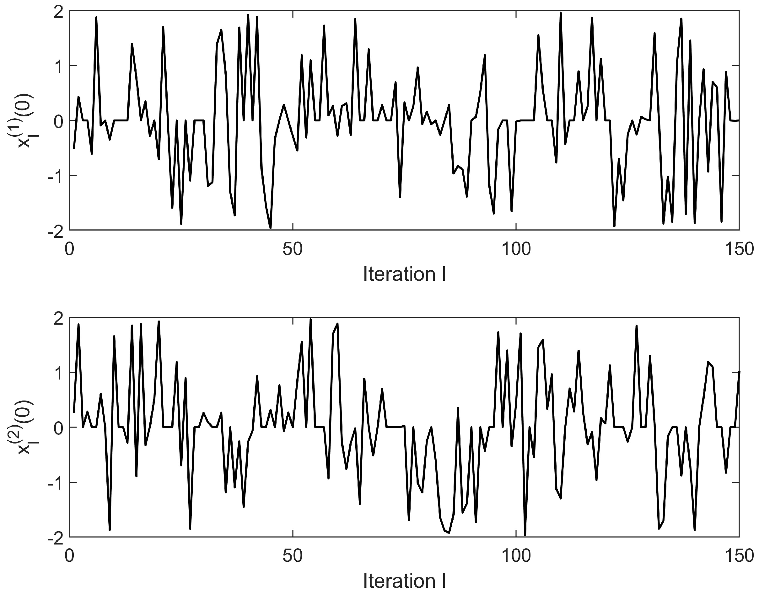
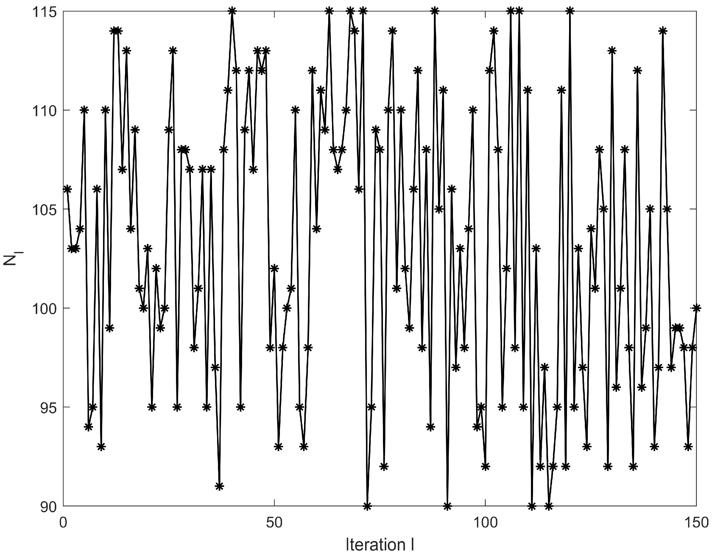
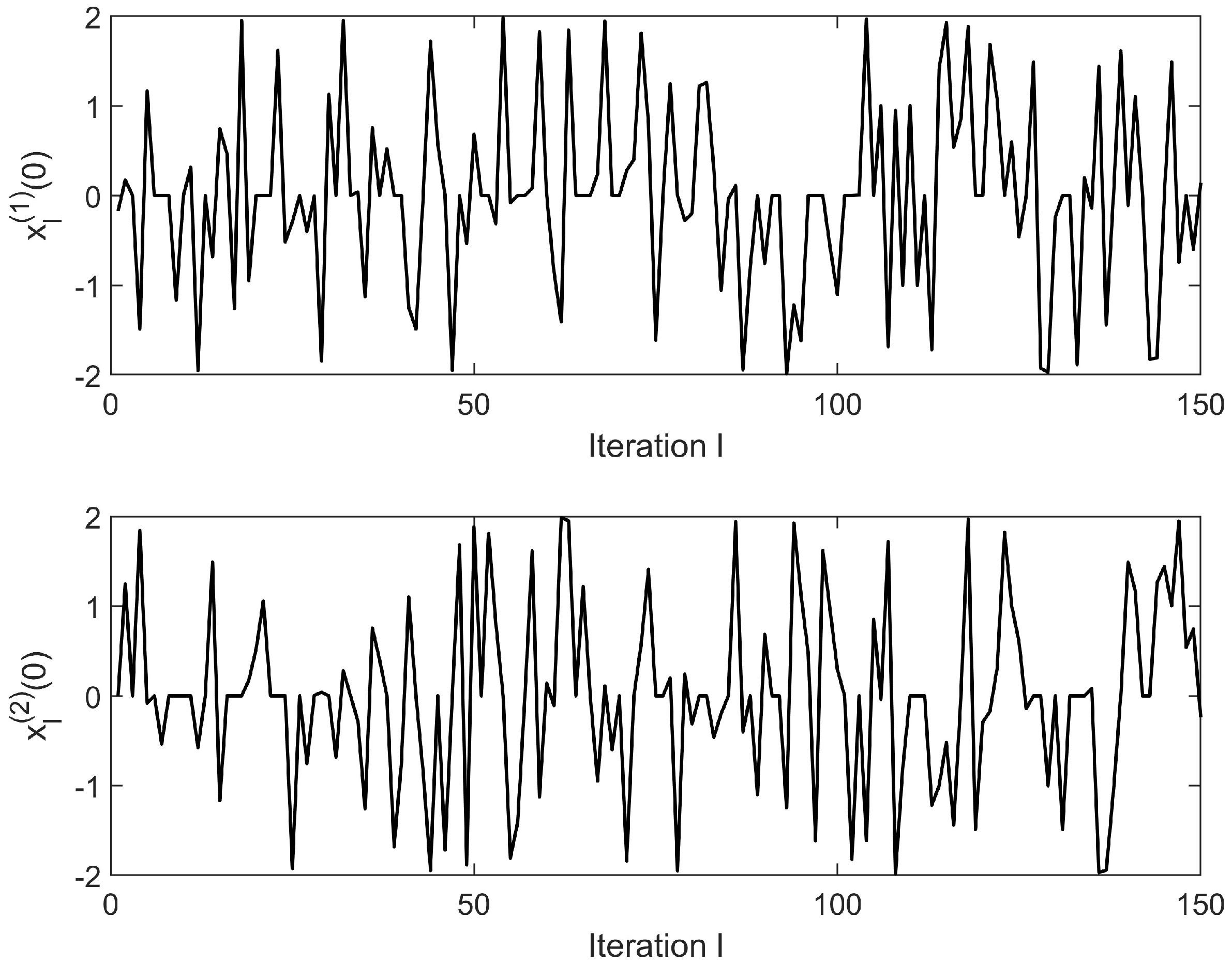
4. Illustrative Example

To validate the boundedness, convergence, and robustness of the control law proposed in the preceding section, we have developed a non-repetitive system as an experimental testbed. The system performance is systematically evaluated through meticulously designed open-loop and closed-loop control strategies, which will be comprehensively elaborated in this section.

Since the system in this study is a dual-variable (time-varying and iteration-varying) dynamics system, the system matrices $A_l\left(t\right)$ and $B_l\left(t\right)$ in the system Equation (1) are configured in the simulation parameters to incorporate dependencies on both time $t$ and iteration count $l$. For the iteration-varying aspect, this is simplified by assigning distinct expressions for even and odd iterations.

Example 1.

To better model the complexities that may be encountered in real-world applications, we assume that the values of the system Equation (1) parameter matrix $A_l\left(t\right)$, $B_l\left(t\right)$, $C_l\left(t\right)$  are

$$A_l\left(t\right)=\left\{\begin{array}{ll}\left[\begin{array}{cc}0.38& 0\\ 0.65& {\left(0.0015t\right)}^2\end{array}\right],\hfill & \forall k,\forall \mathrm{even}l\hfill \\ \left[\begin{array}{cc}0.4& 0\\ 0.68& {\left(0.001t\right)}^2\end{array}\right],\hfill & \forall k,\forall \mathrm{odd}l.\hfill \end{array}\right.$$

(28)

$$B_l\left(t\right)=\left\{\begin{array}{cc}\left[\begin{array}{cc}0.2\sin \left(0.6t\right)& 0.8\\ 5.8& 0.08\cos (0.2t-1)\end{array}\right],& \forall k,\forall \mathrm{even}l\\ \left[\begin{array}{cc}0.1{\sin }^2\left(0.6t\right)& 0.79\\ 5.6& 0.08\cos (0.2t-1)\end{array}\right],& \forall k,\forall \mathrm{odd}l.\end{array}\right.$$

(29)

$$C_l\left(t\right)=\left[\begin{array}{cc}1& 0\\ 0& 1\end{array}\right]$$

(30)

The nonlinear terms ${\left(0.0015t\right)}^2$ and ${\left(0.001t\right)}^2$ are introduced to model slow cumulative effects such as equipment aging and parameter drift. Time-dependent sine and cosine terms are introduced to simulate periodic disturbances in real-world systems, such as mechanical vibrations, thermal fluctuations, and parameter drift. $C_l\left(t\right)$ avoids the complexity of time- or iteration-varying output mappings, ensuring that tracking errors directly reflect state deviations and enhance the interpretability of the results.

As can be observed, the values of parameters $A_l\left(t\right)$ and $B_l\left(t\right)$ evolve with iteration counts, characterizing the system as a dual-varying dynamic with disturbances. The disturbance term $w_l\left(t\right)$ and ${\upsilon }_l\left(t\right)$ is stochastically sampled from interval $\left[-0.002,0.002\right]$ to emulate the minor variations arising from machine inaccuracies in real-world applications. The successful validation through numerical simulations under this configuration convincingly demonstrates the robustness of the implemented open-loop and closed-loop control laws when deployed in non-repetitive systems.

Under the condition that the convergence requirements are met, the values of the gain matrix are provided as follows:

$$\left\{\begin{array}{l}P=\left[\begin{array}{ll}0.04\hfill & 0.07\hfill \\ 0.07\hfill & 0.01\hfill \end{array}\right]\hfill \\ T=\left[\begin{array}{ll}0.03\hfill & 0.02\hfill \\ 0.09\hfill & 0.05\hfill \end{array}\right]\hfill \end{array}\right.$$

(31)

The components $r^{\left(1\right)}\left(t\right)$ and $r^{\left(2\right)}\left(t\right)$ of the reference trajectory $r\left(t\right)$ are defined as follows:

$$r\left(t\right)=\left[\begin{array}{c}{r}^{\left(1\right)}\left(t\right)\\ r^{\left(2\right)}\left(t\right)\end{array}\right]=\left[\begin{array}{c}-0.01t\left[1+\cos \left({\displaystyle \frac{\pi t}{25}}-\pi \right)\right]\\ -0.5\left[1+\sin \left({\displaystyle \frac{\pi t}{50}}-\pi /2\right)\right]\end{array}\right]$$

(32)

$y_l^{\left(i\right)}\left(t\right)\left(i=1,2\right)$ is the component of the output $y_l\left(t\right)=\left[\begin{array}{c}{y}_l^{\left(1\right)}\left(t\right)\\ y_l^{\left(2\right)}\left(t\right)\end{array}\right]$. In order to assess the precision of the ILC tracking of the system, the following error function is constructed:

$$C{E}_l^{\left(i\right)}={\displaystyle \sum _{t=0}^{N_d+1}\left|E\left\{r^{\left(i\right)}\left(t\right)-y_l^{\left(i\right)}\left(t\right)\right\}\right|,i}=1,2$$

(33)

This function evaluates performance by calculating the absolute difference between the system output and the expected output for each iteration, summing these differences while accounting for randomness and uncertainty to ensure robustness.

The open–closed loop law is implemented in the constructed non-repetitive system with iteration count $l=150$ . The temporal variable $t$ is defined over the discrete domain $t\in \left(1,2\cdots \cdots ,N_l\right)$, where $N_l\in \left(90,91,\cdots \cdots ,115\right)$ denotes stochastically varied trajectory lengths across iterations. $x_l^{\left(i\right)}\left(t\right)\left(i=1,2\right)$ is the component of the state $x_l\left(t\right)=\left[\begin{array}{c}{x}_l^{\left(1\right)}\left(t\right)\\ x_l^{\left(2\right)}\left(t\right)\end{array}\right]$ . To validate the robustness against initial state deviations, the iterative initial states $x_l^{\left(1\right)}\left(0\right)$ and $x_l^{\left(2\right)}\left(0\right)$ are randomly initialized within the interval $\left[-2, 2\right]$, with their variations illustrated in Figure 1. Figure 2 presents the dynamic variation in trajectory length $N_l$ during iterations, where $N_l$ varies randomly within the range of 90 to 115.

Apply the ILC law (9)–(11) open–closed loop into system (1). A comparative analysis between the output trajectories and the desired trajectory at iteration counts $l=15$ and $l=20$ is depicted in Figure 3. Notably, the output trajectories progressively approach the desired trajectory as the iteration number increases. Figure 4 demonstrates the evolution of tracking error $C{E}_l^{\left(i\right)}$ versus iteration count $l$, revealing a rapid decline in error magnitude followed by gradual stabilization. This phenomenon substantiates that the open–closed loop system maintains robust learning capability and disturbance resilience even when applied to non-repetitive systems with external disturbances.

Example 2.

Consider a linear piezoelectric motor system with iteratively variable trail lengths and disturbances, which can be described as the following system:

$$\left\{\begin{array}{c}{\dot{\widehat{x}}}_l^{\left(1\right)}\left(\widehat{t}\right)={\widehat{x}}_l^{\left(2\right)}\left(\widehat{t}\right)\\ {\dot{\widehat{x}}}_l^{\left(2\right)}\left(\widehat{t}\right)=-{\displaystyle \frac{K_v}{\overline{M}}}{\widehat{x}}_l^{\left(2\right)}\left(\widehat{t}\right)\\ \widehat{y}\left(t\right)={\widehat{x}}_l^{\left(1\right)}\left(\widehat{t}\right)\end{array}\right.+{\displaystyle \frac{K_f}{M}}{\widehat{u}}_l\left(\widehat{t}\right)$$

(34)

where ${\widehat{x}}_l^{\left(1\right)}\left(\widehat{t}\right)$ and  ${\widehat{x}}_l^{\left(2\right)}\left(\widehat{t}\right)$ are the motion position and the motion velocity, respectively; $\overline{M}=1 \mathrm{kg}$ is the moving mass; $K_v=80 \mathrm{N}$ is the velocity damping factor; and $K_f=6 \mathrm{N}/\mathrm{V}$ is the force constant. Let $u_l\left(t\right)={\widehat{u}}_l\left(t·T_s\right)$, $y_l\left(t\right)={\widehat{y}}_l\left(t·T_s\right)$, and $x_l\left(t\right)={\left[x_l^{\left(1\right)}\left(t\right)x_l^{\left(2\right)}\left(t\right)\right]}^T=$${\left[{\widehat{x}}_l^{\left(1\right)}\left(t·T_s\right){\widehat{x}}_l^{\left(2\right)}\left(t·T_s\right)\right]}^T$ . By adopting  ${\dot{\widehat{x}}}_l^{\left(i\right)}\left(t·T_s\right)\approx ($${\widehat{x}}_l^{\left(i\right)}\left(\left(t+1\right)\right.$$\left.·T_s\right)$$\left.-{\widehat{x}}_l^{\left(i\right)}\left(t·T_s\right)\right)$$/T_s$ for $i=1,2$, we discretize the linear piezoelectric motor system (34) as follows:

$$\left\{\begin{array}{c}{x}_l\left(t+1\right)=\left[\begin{array}{c}1\\ 0\end{array}\left.\begin{array}{c}{T}_s\\ 1-{\displaystyle \frac{K_v{T}_s}{\overline{M}}}\end{array}\right]\right.x_l\left(t\right)+\left[\begin{array}{c}0\\ {\displaystyle \frac{K_v{T}_s}{\overline{M}}}\end{array}\right]u_l\left(t\right)+{\omega }_l\left(t\right)\\ y_l\left(t\right)=\left[0 1\right]x_l\left(t\right)+{\upsilon }_l\left(t\right)\end{array}\right.$$

(35)

where $T_s$ is the sampling time. Take the value $T_s=0.01$ when the number of iterations is even and $T_s=0.015$ when the number of iterations is odd. The reference trajectory is described $r\left(t\right)=-0.5\left(1+\sin \left(\pi t/50-\pi /2\right)\right)$, where $t\in \left\{0,1,\cdots ,200\right\}$ with $N_d=200$ . To validate the robustness against initial state deviations, the iterative initial states $x_l^{\left(1\right)}\left(0\right)$ and $x_l^{\left(2\right)}\left(0\right)$ are randomly initialized within the interval $\left[-2, 2\right]$, with their variations illustrated in Figure 5. The iteratively varying trail length $N_l$ in (35) varies between 187 and 210 as shown in Figure 6. The initial control input $u_0\left(t\right)=0$$t\in \left\{0,1,\cdots ,200\right\}$ and the initial state $E\left\{x_l\left(0\right)\right\}=x_d\left(0\right)={\left[0 0\right]}^T$ . The disturbance terms $w_l\left(t\right)$ and ${\upsilon }_l\left(t\right)$ are stochastically sampled from interval $\left[-0.002,0.002\right]$ to emulate the minor variations arising from machine inaccuracies in real-world applications. The following tracking error index is used to evaluate the ILC performance

$$H{E}_l={\displaystyle \sum _{t=0}^{N_d+1}\left|E\left\{r\left(t\right)-y_l\left(t\right)\right\}\right|}$$

(36)

The open–closed loop law is implemented in the constructed non-repetitive system with iteration count $l=150$. $P=0.75, L=0.6$. Figure 7 displays the tracking performance of the system output $y_l\left(t\right)$ to the reference trajectory $r\left(t\right)=-0.5\left(1+\sin \left(\pi t/50-\pi /2\right)\right)$ at iterations $l=15$ and $l=35$ with the open–closed loop ILC law (9)–(11). It is shown in Figure 7 that a progressively improved tracking situation of system output $y_l\left(t\right)$ to reference trajectory $r\left(t\right)$ is obtained. Figure 8 shows the performance index $H{E}_l$ at different iterations. The ILC tracking error converges to a small neighborhood in the sense of mathematical expectation.

5. Conclusions

This study proposes a novel open–closed loop composite robust ILC framework for MIMO linear discrete-time systems subject to multiple-source non-repetitive uncertainties. The framework incorporates a Bernoulli-distributed stochastic variable to address trajectory variations and an open–closed loop law to ensure tracking error convergence to a small neighborhood under multi-source non-repetitive conditions, including two-dimensional temporal–iterative model variations, stochastic trajectory length fluctuations, non-repetitive disturbances, and initial state deviations. The simulation results demonstrate that under randomized initial states and trajectory lengths, the tracking error rapidly decreases and tends to stabilize after approximately 40 iterations, ultimately converging to the desired trajectory. Further simulation on a real system, a piezoelectric motor system, verifies that the ILC tracking error converges to a small neighborhood in the sense of mathematical expectation. The proposed method exhibits strong learning capability, robustness, and stability, thereby offering an effective solution for controlling non-repetitive systems while providing valuable insights for theoretical research and practical applications.

References

1. Duran, O.; Garcia-Tabares, L.; Gonzalez, L.A.; Toral, F.; Arimoto, Y.; Yamada, T.; Yamamoto, A. Conceptual Design of a Conduction-Cooled Superconducting Quadrupole for ILC Main Linac With Large Temperature Margin. IEEE Trans. Appl. Supercond. 2025, 3, 4003605. [Google Scholar] [CrossRef]
2. Yang, R.; Gong, Y.; Paszke, W. ILC-Based Tracking Control for Linear Systems With External Disturbances via an SMC Scheme. IEEE Trans. Autom. Sci. Eng. 2025, 22, 9698–9707. [Google Scholar] [CrossRef]
3. Gao, K.; Zhou, Y.; Gao, F.; Lu, J. Optimally Selected Cycle-Based ILC for System With Randomly Varying Initial State. IEEE Trans. Autom. Control. 2025, 70, 2714–2721. [Google Scholar] [CrossRef]
4. Liu, S.Y.; Meng, D.Y.; Cheng, L.; Chen, M. An Iterative Learning Controller for A Cable-Driven Hand Rehabilitation Robot. In Proceedings of the 43rd Annual Conference of the IEEE-Industrial-Electronics-Society (IECON), Beijing, China, 29 October–1 November 2017; pp. 5701–5706. [Google Scholar]
5. He, W.; Meng, T.T.; Huang, D.Q.; Li, X.F. Adaptive Boundary Iterative Learning Control for an Euler-Bernoulli Beam System with Input Constraint. IEEE Trans. Neural Netw. Learn. Syst. 2018, 29, 1539–1549. [Google Scholar] [CrossRef]
6. Zhang, S.Y.; Wang, L.; Wang, H.H.; Xue, B. Consensus Control for Heterogeneous Multivehicle Systems: An Iterative Learning Approach. IEEE Trans. Neural Netw. Learn. Syst. 2021, 32, 5356–5368. [Google Scholar] [CrossRef]
7. Huang, J.S.; Wang, W.; Su, X.J. Adaptive Iterative Learning Control of Multiple Autonomous Vehicles With a Time-Varying Reference Under Actuator Faults. IEEE Trans. Neural Netw. Learn. Syst. 2021, 32, 5512–5525. [Google Scholar] [CrossRef]
8. Hui, Y.; Chi, R.H.; Huang, B.; Hou, Z.S. Extended State Observer-Based Data-Driven Iterative Learning Control for Permanent Magnet Linear Motor With Initial Shifts and Disturbances. IEEE Trans. Syst. Man Cybern. Syst. 2021, 51, 1881–1891. [Google Scholar] [CrossRef]
9. Meng, D.Y.; Zhang, J.Y. Convergence Analysis of Robust Iterative Learning Control Against Nonrepetitive Uncertainties: System Equivalence Transformation. IEEE Trans. Neural Netw. Learn. Syst. 2021, 32, 3867–3879. [Google Scholar] [CrossRef]
10. Guth, M.; Seel, T.; Raisch, J. Iterative Learning Control with Variable Pass Length Applied to Trajectory Tracking on a Crane with Output Constraints. In Proceedings of the 52nd IEEE Annual Conference on Decision and Control (CDC), Florence, Italy, 10–13 December 2013; pp. 6676–6681. [Google Scholar]
11. Yu, Q.X.; Hou, Z.S. Adaptive Fuzzy Iterative Learning Control for High-Speed Trains With Both Randomly Varying Operation Lengths and System Constraints. IEEE Trans. Fuzzy Syst. 2021, 29, 2408–2418. [Google Scholar] [CrossRef]
12. Nagy, Z.K. Model based robust control approach for batch crystallization product design. Comput. Chem. Eng. 2009, 33, 1685–1691. [Google Scholar] [CrossRef]
13. Butcher, M.; Karimi, A. Linear Parameter-Varying Iterative Learning Control With Application to a Linear Motor System. IEEE-Asme Trans. Mechatron. 2010, 15, 412–420. [Google Scholar] [CrossRef]
14. Liu, T.; Gao, F.R. Robust two-dimensional iterative learning control for batch processes with state delay and time-varying uncertainties. Chem. Eng. Sci. 2010, 65, 6134–6144. [Google Scholar] [CrossRef]
15. Yu, M.; Chai, S. Iteration-dependent High-order Internal Model based Iterative Learning Control for Discrete-time Nonlinear Systems with Time-iteration-varying Parameter. In Proceedings of the 21st IFAC World Congress on Automatic Control—Meeting Societal Challenges, Berlin, Germany, 11–17 July 2020; pp. 1658–1663. [Google Scholar]
16. Wang, L.; Huangfu, Z.W.; Li, R.W.; Wen, X.W.; Sun, Y.; Chen, Y.Y. Iterative learning control with parameter estimation for non-repetitive time-varying systems. J. Frankl. Inst. 2024, 361, 1455–1466. [Google Scholar] [CrossRef]
17. He, C.; Li, J.M.; Liu, S.Y.; Wang, J.X. Robust model-based predictive iterative learning control for systems with non-repetitive disturbances. Nonlinear Anal. Hybrid Syst. 2024, 51, 101436. [Google Scholar] [CrossRef]
18. Chen, Y.Y.; Jiang, W.; Charalambous, T. Machine learning based iterative learning control for non-repetitive time-varying systems. Int. J. Robust Nonlinear Control 2023, 33, 4098–4411. [Google Scholar] [CrossRef]
19. Liu, T.; Hao, S.L.; Wang, Y.Q.; Na, J. Predictive State Observer-Based Set-Point Learning Control for Batch Manufacturing Processes With Delay Response. IEEE Trans. Ind. Electron. 2024, 71, 788–797. [Google Scholar] [CrossRef]
20. Fu, W.Y. Frequency-domain-based nonlinear normalized iterative learning control for three-dimensional ball screw drive systems. Isa Trans. 2025, 157, 224–232. [Google Scholar]
21. Chai, S.; Yu, M.; Zhao, K. Robust adaptive event-triggered ILC scheme design for discrete-time non-repetitive nonlinear systems. Iet Control. Theory Appl. 2024, 18, 213–228. [Google Scholar] [CrossRef]
22. Yu, Y.R.; Li, D.W.; Ma, A.Y.; Gao, F.R. Sliding Mode-Based Two-Dimensional Iterative Learning Control for Systems with Uncertainties and External Disturbances. In Proceedings of the IEEE 18th International Conference on Control and Automation (ICCA), Reykjavik, Iceland, 18–21 June 2024; pp. 641–646. [Google Scholar]
23. Zhang, J.Y.; Meng, D.Y. Improving Tracking Accuracy for Repetitive Learning Systems by High-Order Extended State Observers. IEEE Trans. Neural Netw. Learn. Syst. 2023, 34, 10398–10407. [Google Scholar] [CrossRef]
24. Wan, K.; Xie, H.; Xu, Q.Y. Robust Iterative Learning Control for 2-D Linear Nonrepetitive Discrete Systems With Iteration-Dependent Trajectory. IEEE Access 2022, 10, 125015–125026. [Google Scholar] [CrossRef]
25. Barkhordar-pour, H.; Lim, J.G.; Ben Ayed, A.; Mitran, P.; Boumaiza, S. Linearizability Assessment of a 3.5 GHz 16-Chain Fully Digital MIMO Transmitter Under Wideband Modulated Signals. In Proceedings of the 103rd ARFTG Microwave Measurement Conference (ARFTG) on Advanced Measurement Techniques for Next-G Communication Systems, Washington, DC, USA, 21 June 2024. [Google Scholar]
26. Kwon, G.; Liu, Z.; Conti, A.; Park, H.; Win, M.Z. Integrated Localization and Communication for Efficient Millimeter Wave Networks. IEEE J. Sel. Areas Commun. 2023, 41, 3925–3941. [Google Scholar] [CrossRef]
27. Zhang, Z.; Zou, Q. Data-driven robust iterative learning control of linear systems. Automatica 2024, 164, 111646. [Google Scholar] [CrossRef]
28. Aarnoudse, L.; Oomen, T. Random Learning Leads to Faster Convergence in ‘Model-Free’ ILC: With Application to MIMO Feedforward in Industrial Printing. Int. J. Adapt. Control. Signal Process. 2024. [Google Scholar] [CrossRef]
29. Song, E.J.; Baek, S.G.; Oh, D.J.; Beak, J.M.; Koo, J.C. ILC-driven control enhancement for integrated MIMO soft robotic system. Intell. Serv. Robot. 2024, 17, 357–368. [Google Scholar] [CrossRef]
30. Wei, Y.S.; Li, X.D. Robust higher-order ILC for non-linear discrete-time systems with varying trail lengths and random initial state shifts. Iet Control Theory Appl. 2017, 11, 2440–2447. [Google Scholar] [CrossRef]
Figure 1. Initial state variations in x l 1 0 and x l 2 0 across iterative steps.
Mathematics 13 01675 g001
Figure 2. Dynamically adjusted trail length N l in system (1) over successive iterations.
Mathematics 13 01675 g002
Figure 3. Output characteristics y l i t i = 1 , 2 at iterations l = 15 and l = 20 , implemented via the open–closed loop ILC law (9)–(11).
Mathematics 13 01675 g003
Figure 4. Evolution of ILC tracking error C E l i i = 1 , 2 across multiple iterations under the open–closed loop ILC law (9)–(11).
Mathematics 13 01675 g004
Figure 5. Initial state variations in x l 1 0 and x l 2 0 across iterative steps.
Mathematics 13 01675 g005
Figure 6. Iteration-dependent adjustments of trail length N l in system (35).
Mathematics 13 01675 g006
Figure 7. Temporal profiles of system outputs y l   t at iterations l = 15 and l = 35 , implemented via the open–closed loop ILC law (9)–(11).
Mathematics 13 01675 g007
Figure 8. Iteration-wise trends of ILC tracking error H E l across multiple iterations under the open–closed loop ILC law (9)–(11).
Mathematics 13 01675 g008
Disclaimer/Publisher’s Note: The statements, opinions and data contained in all publications are solely those of the individual author(s) and contributor(s) and not of MDPI and/or the editor(s). MDPI and/or the editor(s) disclaim responsibility for any injury to people or property resulting from any ideas, methods, instructions or products referred to in the content.