1. Introduction
The intensification of industrialization and urbanization has exacerbated global water scarcity and pollution, positioning wastewater treatment and water quality optimization as pivotal challenges in environmental sustainability and resource recovery [
1]. Internationally, water resource management has gained unprecedented policy emphasis, notably reflected in the United Nations Sustainable Development Goals (SDGs) that mandate urgent actions on clean water accessibility and aquatic ecosystem preservation [
2,
3].
Conventional control strategies in wastewater treatment, particularly Proportional-Integral-Derivative (PID) control, dominate industrial applications owing to their simplicity and cost-effectiveness for linear systems [
4]. However, PID controllers are inherently limited in handling nonlinear dynamics, time-varying disturbances, and high-dimensional processes, often necessitating laborious parameter calibration to mitigate performance deterioration [
5]. In contrast, Model Predictive Control (MPC) offers a systematic framework for handling multivariable nonlinear systems through receding horizon optimization, enabling global performance guarantees while explicitly accommodating constraints [
6]. These advantages have spurred MPC’s adoption in wastewater treatment plants (WWTPs). For instance, Lin Yonggang et al. [
7] applied MPC to optimize multipump station scheduling in sewage systems, effectively reducing complexity and costs. Martin M. et al. [
8] implemented MPC in controlling cascaded bioreactors at wastewater treatment plants, achieving satisfactory performance with reduced steady-state errors. Economic Model Predictive Control (EMPC), an advanced variant of MPC, extends these benefits by directly incorporating economic objectives (e.g., energy minimization, operational cost reduction) into the optimization framework [
9]. As evidenced by Zeng et al. [
10], EMPC surpasses conventional PI and MPC in simultaneously enhancing effluent quality and lowering operational expenses. Nevertheless, deploying EMPC on high-fidelity models such as the Benchmark Simulation Model No. 1 (BSM1) entails solving computationally intensive nonlinear optimization problems at each sampling interval, posing prohibitive online computation demands for real-time implementation. Thus, reducing computation time is crucial for improving efficiency. To address this, scholars have proposed various methods to lower computational complexity. For example, Zhang et al. [
11] introduced a distributed EMPC strategy, which enhanced effluent quality and energy efficiency through system-wide model design.
Model order reduction (MOR) techniques provide a systematic pathway to alleviate computational complexity. Among these, Trajectory Piecewise Linearization (TPWL) has emerged as a promising strategy that approximates nonlinear dynamics through locally linearized models along system trajectories [
12]. By strategically selecting linearization points, TPWL enables tunable trade-offs between approximation accuracy and computational efficiency, making it particularly suited for real-time control of large-scale systems. For instance, Zhang et al. [
13] applied TPWL to EMPC in wastewater treatment plants, demonstrating substantial improvements in computational efficiency through model approximation.
Proper Orthogonal Decomposition (POD), a common dimensionality reduction technique [
14,
15,
16], has also been widely used in model simplification. By reducing the dimensionality of wastewater treatment plants (WWTPs) models and integrating TPWL, further simplification can be achieved.
The global maximum error control (GMEC) method iteratively refines approximate models by identifying and addressing the maximum error points during simulation until error thresholds are met.
Building on these advancements, this paper proposes a reduced-order TPWL-based EMPC framework integrated with GMEC for wastewater treatment plants. First, candidate linearization points are selected from the state trajectory of the original nonlinear model using TPWL. A reduced-order model is then constructed via POD, followed by TPWL simplification. During TPWL, linearization points are dynamically selected from the candidate pool using GMEC to ensure the maximum error of the simplified model meets predefined thresholds. Finally, the simplified model’s performance—including error magnitude, control efficacy, and computation time—is analyzed.
This study introduces a novel EMPC framework combining GMEC, TPWL, and POD (GMEC-POD-TPWL-EMPC), addressing the low computational efficiency of traditional EMPC in nonlinear wastewater treatment models. A two-stage linearization point selection strategy optimizes TPWL efficiency, overcoming the empirical limitations of traditional TPWL highlighted in [
12,
13]. Furthermore, by integrating POD, this work extends its application from fluid dynamics [
14,
15,
16] to wastewater treatment control, offering new insights for real-time control of large-scale nonlinear systems.
An error feedback-based adaptive model simplification mechanism is developed, dynamically adjusting linearization point distribution via GMEC to balance computational efficiency and control accuracy. Compared with the single-point selection in [
13], this paper’s dual-stage strategy combines state trajectory spacing with global error thresholds, minimizing redundant points and validating its applicability in complex industrial scenarios. Using BSM1 as a case study, the method’s effectiveness in high-dimensional nonlinear systems is demonstrated.
Additionally, this approach provides an efficient tool for real-time wastewater control. Experiments show that under controllable performance losses (e.g., effluent quality, energy consumption), the proposed method achieves optimization speeds meeting real-time requirements, outperforming traditional EMPC (e.g., the distributed strategy in [
9,
11] incurs extra communication costs). It quantifies the relationship between linearization points and computational efficiency, offering theoretical guidance for parameter tuning in industrial settings. Unlike intelligent control methods in [
5,
6], which rely on high-performance computing, this method reduces EMPC complexity, enabling deployment in resource-limited wastewater treatment plants.
2. Model Description
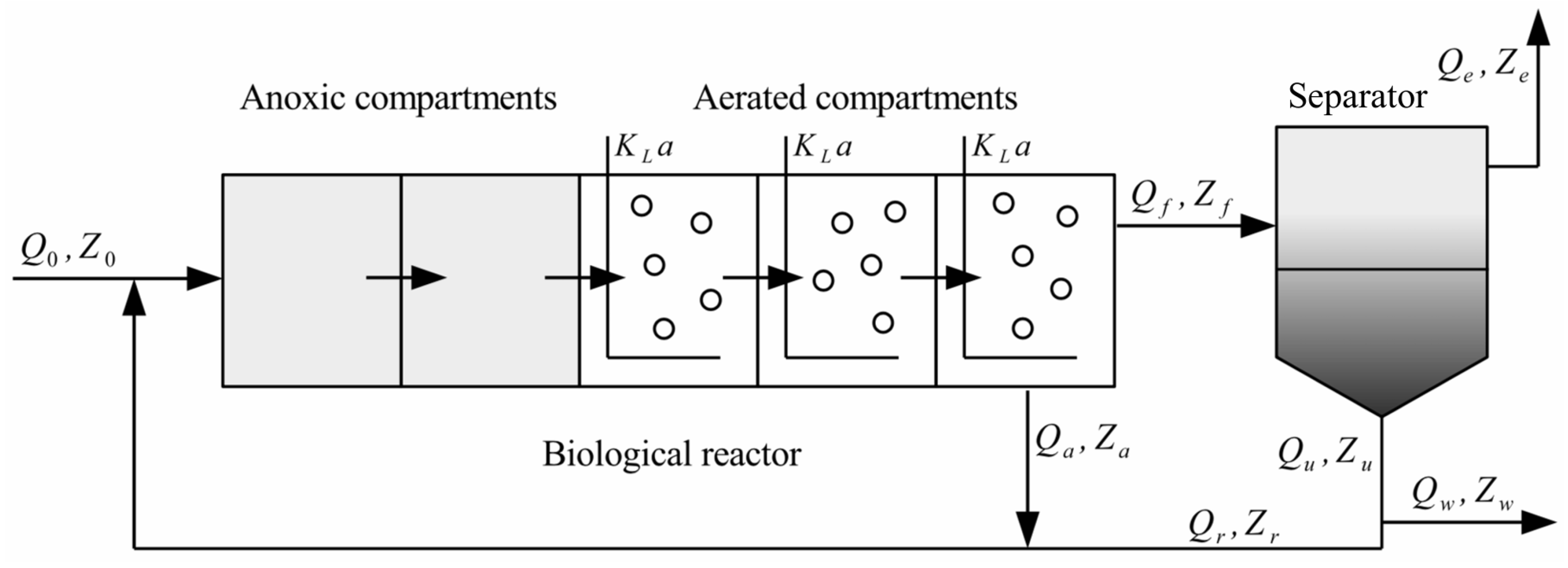
The wastewater treatment system analyzed in this study employs an enhanced configuration derived from the Benchmark Simulation Model No. 1 (BSM1), with schematic representation and parameter specifications provided in
Figure 1 and
Table 1, respectively. The system integrates a five-compartment sludge reactor coupled with an ideal secondary clarifier [
17]. Biochemical reactions within the reactor are spatially segregated: denitrification is facilitated in the first two anoxic compartments, where nitrate reduction generates nitrogen gas, while nitrification dominates the subsequent three aerobic compartments, enabling ammonia oxidation to nitrate.
Hydraulic inputs to the primary reactor compartment include three distinct streams: (1) raw influent with volumetric flow rate
and pollutant concentration
; (2) internal recirculation flow (
,
) recycled from the terminal aerobic compartment; and (3) external recirculation flow (
,
) extracted from the clarifier underflow. The clarifier partitions the reactor effluent into two streams: purified overflow discharge (
,
) and underflow sludge withdrawal (
,
). A residual flow (
,
) from the final aerobic compartment directly feeds the clarifier. The process dynamics are governed by eight core biochemical reaction mechanisms [
18].
The modified BSM1-based wastewater treatment process is mathematically represented by a system of 78 coupled ordinary differential equations (ODEs). Each reactor compartment and the ideal secondary clarifier [
19] are governed by 13 interdependent state variables, each associated with a distinct differential equation. These variables, comprehensively detailed in
Table 2, encompass critical parameters such as substrate concentrations, biomass dynamics, and dissolved oxygen levels, collectively defining the system’s transient behavior.
For the first biological reaction chamber (
k = 1):
For the second to fifth biological reaction chambers (
k = 2, …, 5),
for which the conversion rate
of each component is shown in [
19]. The special case for the concentration of dissolved oxygen is as follows:
Equations (
1), (
3), and (
5) define key parameters governing the biological reactor dynamics:
denotes the dissolved oxygen concentration in the
k-th compartment,
corresponds to the compound concentration (as specified in
Table 2) within the
k-th reactor compartment,
represents compartment volume,
quantifies the compound-specific reaction rate,
is the oxygen saturation constant (fixed at 8
), and
signifies the compartment-specific oxygen transfer coefficient. Notably,
and
are nullified (
) in the anoxic compartments (Compartments 1–2) [
19].
The ideal secondary clarifier [
17] is modeled as a nonbiological membrane filtration unit. Soluble compounds are assumed fully homogenized within the clarifier, while particulate components undergo complete gravitational settling in its lower section [
20].
In this case, the dynamic equation of the separator unit is as follows:
The following are some concentration and flow relationships in the process:
For the WWTP, the modified BSM1 model can be expressed in the following compact form:
where
denotes the state vector encapsulating all process variables, and
corresponds to the input vector comprising both manipulated and exogenous variables. The manipulated inputs include the internal recirculation flow rate
and the oxygen transfer coefficient
in the fifth bioreactor compartment, whereas the influent flow rate
is treated as an uncontrolled disturbance.
The economic control indicators for the model are defined as follows:
where
represents the effluent quality,
denotes the overall cost index, which encompasses factors significantly affecting operational costs,
and
are the weighting coefficients for effluent quality and overall cost index. In this article, EQ
is one of the important performance indicators. It represents the daily average value of the weighted sum of the emission concentrations of chemical substances. The concentrations of these compounds will affect the quality of treated water. EQ index can be described by the following:
where
Equation (
18) defines key evaluation parameters:
and
denote the initial and terminal instants of the assessment interval, respectively, with
representing the evaluation duration (typically
). The effluent quality index (EQ) incorporates constituent concentrations—suspended solids (
), chemical oxygen demand (
), biological oxygen demand (
), and Kjeldahl nitrogen (
)—weighted by coefficients
,
,
,
, and
. Stoichiometric parameters
,
, and
[
21] further refine the model, where subscript
e designates the secondary clarifier effluent.
Operational cost optimization is critical for ensuring the economic sustainability of wastewater treatment. The total operating cost, influenced by multiple factors (summarized in
Table 3), necessitates systematic control strategies to balance process efficiency and financial expenditures.
The sludge production rate, defined as the daily average mass of particulate solids generated during the operational evaluation period
T, comprises two components: (1) particulate discharge via the secondary clarifier’s wastage flow
and (2) accumulated solids retained within the treatment facility. This metric is mathematically expressed as
where subscript
w designates the wastage outlet of the secondary clarifier.
Aeration energy consumption (AE) is influenced by multiple operational and design parameters, including wastewater characteristics, microbial metabolic activity, sludge settling properties, aeration system efficiency, environmental conditions, process configuration, and advanced control strategies. AE is quantified using oxygen transfer rates (
,
) under a standardized immersion depth of 4 m, as defined by
where
represents the volume of the
i-th reactor compartment (
),
denotes the compartment-specific oxygen transfer coefficient, and
is the oxygen saturation concentration (fixed at
).
In the whole sewage treatment process, pumping energy is related to hydraulic characteristics, pumping equipment performance, sewage physical characteristics, process design, and operation strategy. Here, the energy consumed by the pump for internal circulation
and external circulation
is mainly considered, and its mathematical description is as follows:
The mixing energy refers to the energy consumed by mixing compounds in an anoxic chamber to avoid precipitation. The calculation of me depends on the volume of each reaction chamber and the oxygen transfer rate. As shown in (
26), it is positively correlated with the volume of the reaction chamber. Its mathematical expression is as follows:
The overall cost index (OCI) approximates the total cost for WWTP operation by taking a weighted summation of the listed major factors as follows:
5. Design of EMPC Controller Based on Reduced-Order Linearized Model
In the above algorithm, the maximum error control limit is a parameter that needs to be manually given, and its value is related to the approximate accuracy and scale of the final TPWL surrogate model, so it needs to be set according to the actual application requirements.
Unlike existing methods, the proposed GMEC dynamically incorporates new linearization points through a global maximum error feedback mechanism, iteratively refining the TPWL model to ensure balanced accuracy and efficiency. In addition, the existing linearization point selection algorithms are either based on the geometric distance between the state points, the error estimation between the local linearization reduced order model and the original nonlinear model, or the local approximation effect of the linearization function. Existing approaches primarily focus on local approximation accuracy (e.g., geometric proximity or Jacobian linearization fidelity), whereas the proposed GMEC method explicitly enforces global error bounds through iterative refinement.
EMPC extends the receding horizon optimization framework of MPC by embedding economic objectives (e.g., energy cost minimization, operational profit maximization) directly into the optimal control problem. This dual focus enables EMPC to simultaneously regulate dynamic performance (e.g., tracking accuracy, stability margins) and enhance economic efficiency.
MPC solves a finite-horizon optimal control problem iteratively, leveraging system predictions to compute control actions while explicitly handling constraints. Its defining feature—the receding horizon mechanism—applies only the immediate control input and recomputes the sequence at each sampling instant, thereby achieving closed-loop robustness. Economic optimization aims to minimize (or maximize) economic indicators of the system, such as energy consumption, operational costs, and revenue.
EMPC embeds economic optimization objectives directly into the MPC optimization problem, allowing the controller to consider both dynamic performance (e.g., tracking accuracy, stability) and economic performance (e.g., operating costs, energy efficiency).
The design of the EMPC controller based on the reduced-order linearized model, as described by Equation (
38), is formulated as follows:
The EMPC objective function in Equation (
42) minimizes the economic cost
defined in Equation (
17), where
N denotes the prediction horizon,
is the set of piecewise-constant control policies with sampling interval
, and
U encodes input constraints. By solving Equation (
42), the optimal control input
is obtained. The first element of the optimal control sequence is implemented, and the horizon is shifted forward at each sampling instant.
6. Experimental Simulation
6.1. Simulation Parameter Settings
The Trajectory Piecewise Linearization with Proper Orthogonal Decomposition (TPWL-POD) is applied to a wastewater treatment plant (WWTP) model. Based on the given input signals, the reduced-order basis and linearization points of the model are obtained, and the accuracy of the approximated model is compared with that of the original nonlinear model. Considering the influence of weather conditions on the model, this study focuses on evaluating control performance under sunny conditions, including effluent quality, operational costs, and computational efficiency.
The data files for sunny conditions are referenced from the BSM1 benchmark dataset, which is made publicly available by the International Water Association (IWA) [
29]. These files contain the influent flow rate
and influent concentration
. Under sunny conditions, static simulations of the WWTP are conducted using the average values of
and
to determine the optimal steady state, which serves as the initial condition for the wastewater treatment process.
The simulation spans 14 days, with the final 7-day period utilized for performance evaluation. The sampling time is defined as min.
In the economic control objective function (Equation (
17)), the weighting coefficients
and
are set to 1 and 0.3, respectively. For all EMPC controller designs, the control horizon is fixed at 25. The constraints on operational inputs in all control designs are as follows:
where
represents the average influent flow rate under dry weather conditions, which is 18,446 m
3 · d
−1.
The TPWL-POD framework initially selects 60 candidate linearization points. The reduced-order model (ROM) retains 30 dominant states via singular value truncation. Through preliminary simulations, the global maximum error threshold is set to 9 (RMSE), which balances accuracy and computational efficiency and determines the number of linearization points. A smaller threshold leads to more linearization points being selected. The threshold and reduced-order dimensionality are determined based on a trade-off between model accuracy and computational time. This process requires extensive simulations and empirical analysis.
The model’s accuracy increases as the threshold decreases and the reduced-order dimensionality increases. However, computational time also rises accordingly. Balancing model accuracy and computational efficiency is critical for establishing a reliable model. These parameters were carefully tuned to achieve an optimal compromise.
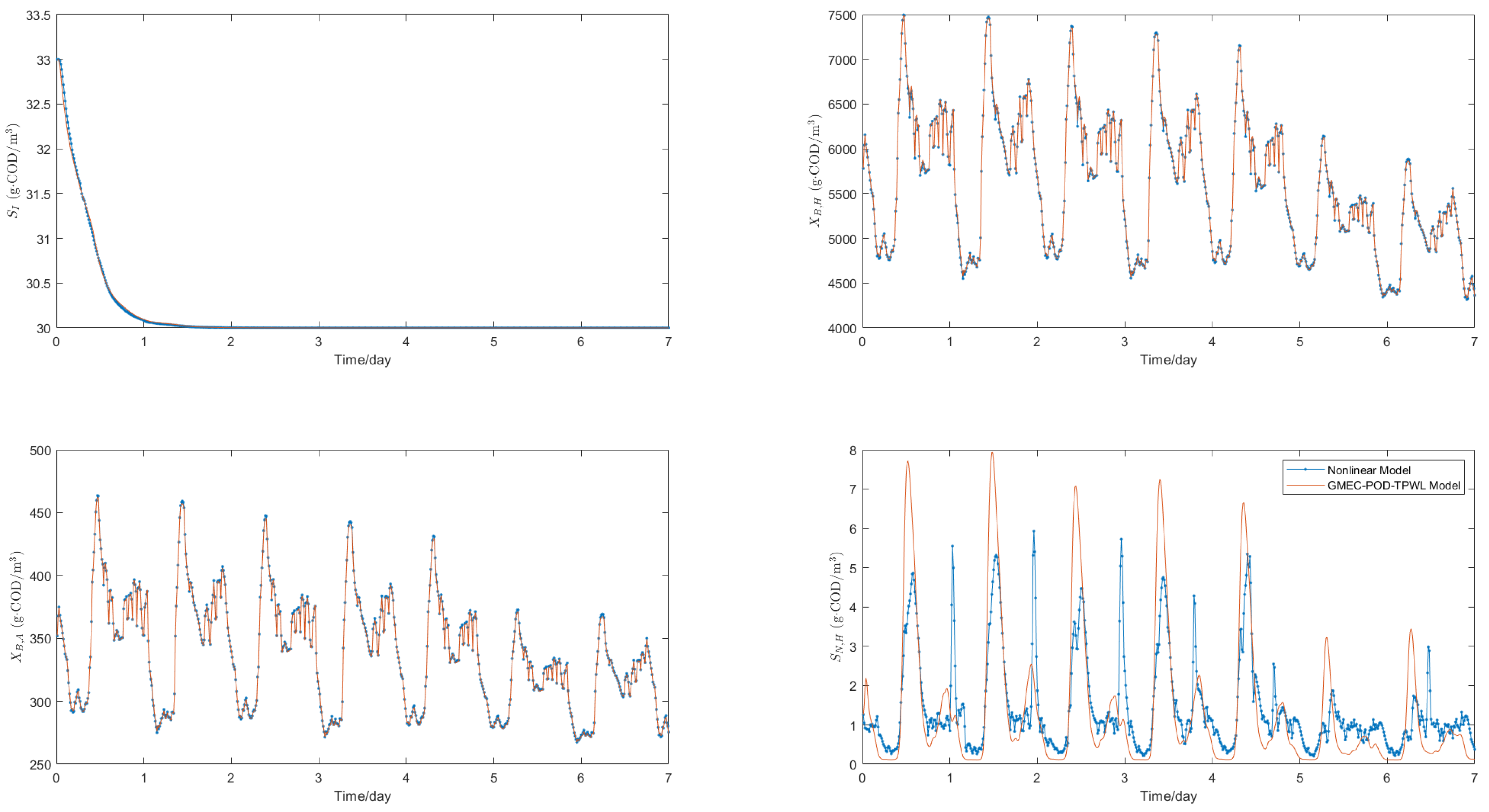
6.2. Model Validation
For both the original nonlinear model and the reduced-order linearized model, the state data generated under identical input signals during the first week are nearly identical. To illustrate this, this study selects four key state variables from the first reaction chamber for comparison: soluble nonbiodegradable organic matter (
), active heterotrophic bacteria (
), active autotrophic bacteria (
), and ammonia nitrogen (
).
Figure 3 compares the temporal evolution of four critical states (
,
,
,
) between the original model and the GMEC-POD-TPWL model. The negligible deviations confirm the GMEC-POD-TPWL model’s fidelity in capturing dominant dynamics.
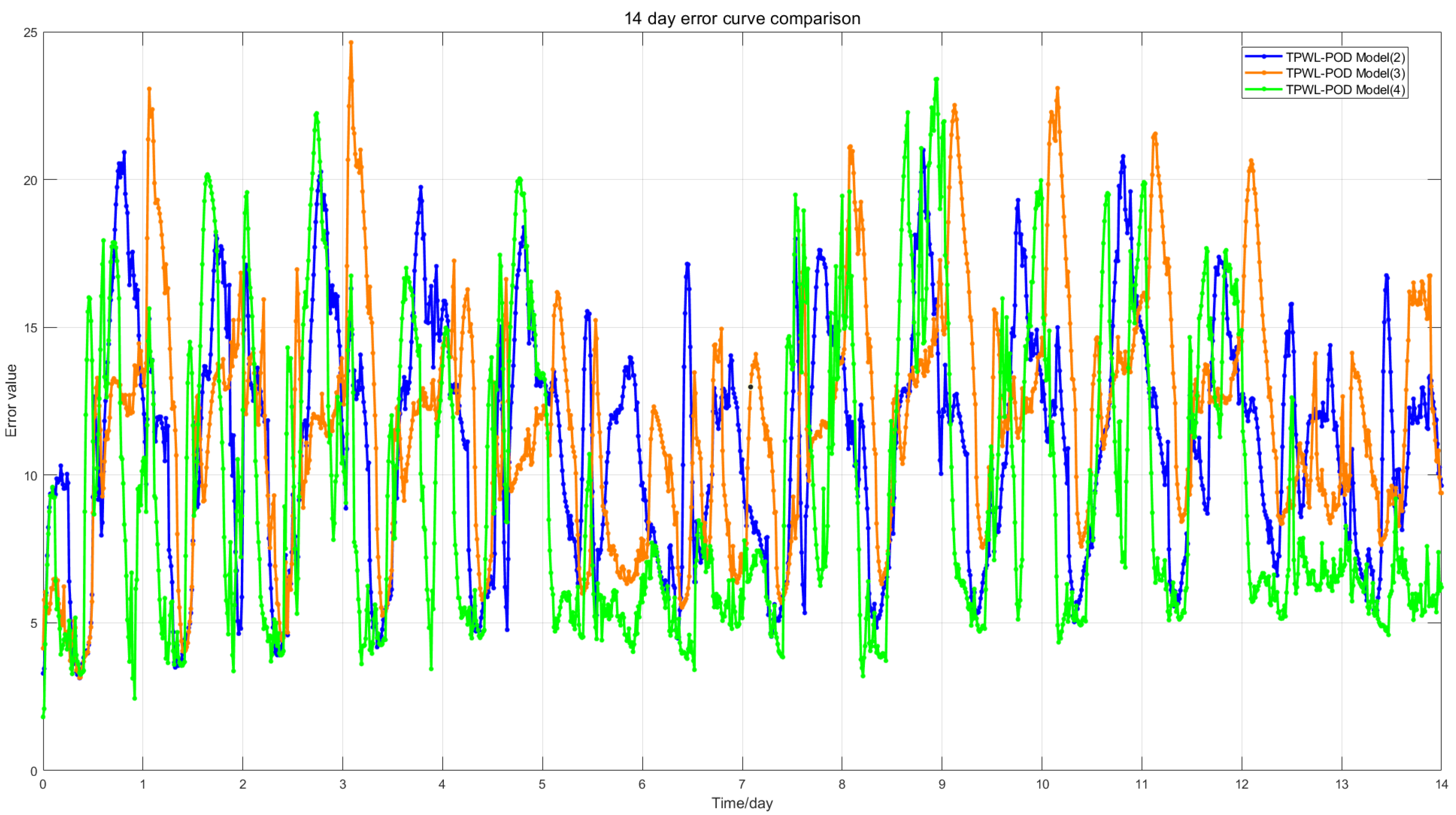
6.3. Model Comparison
To validate the superiority of the proposed Global Maximum Error-based Secondary Point Selection (GMEC-POD-TPWL) modeling method over other TPWL approaches, this study compares its accuracy with the TPWL-POD method from reference [
13] under varying numbers of linearization points (2, 3, and 4). A comparative analysis is conducted, and the results are presented in
Table 4,
Figure 4 and
Figure 5. The error between the reduced-order models and the original model is quantified using the RMSE, calculated as in Equation (
39).
Figure 4 illustrates the RMSE trajectories of the TPWL-POD model compared with the original model over the entire 14-day simulation period, while
Figure 5 shows the corresponding error trajectories for the GMEC-POD-TPWL model.
As demonstrated, the proposed GMEC-POD-TPWL model achieves error reductions of 13.90%, 20.69%, and 44.34% for 2, 3, and 4 linearization points, respectively, compared with the TPWL-POD method. These results highlight a significant enhancement in model accuracy, confirming the effectiveness of the GMEC-based secondary point selection strategy.
The data in
Table 4 indicate that as the linearization point increases, the errors of both models gradually decrease, and under the same linearization point, the error of the GMEC-POD-TPWL model is smaller than that of the TPWL-POD model.
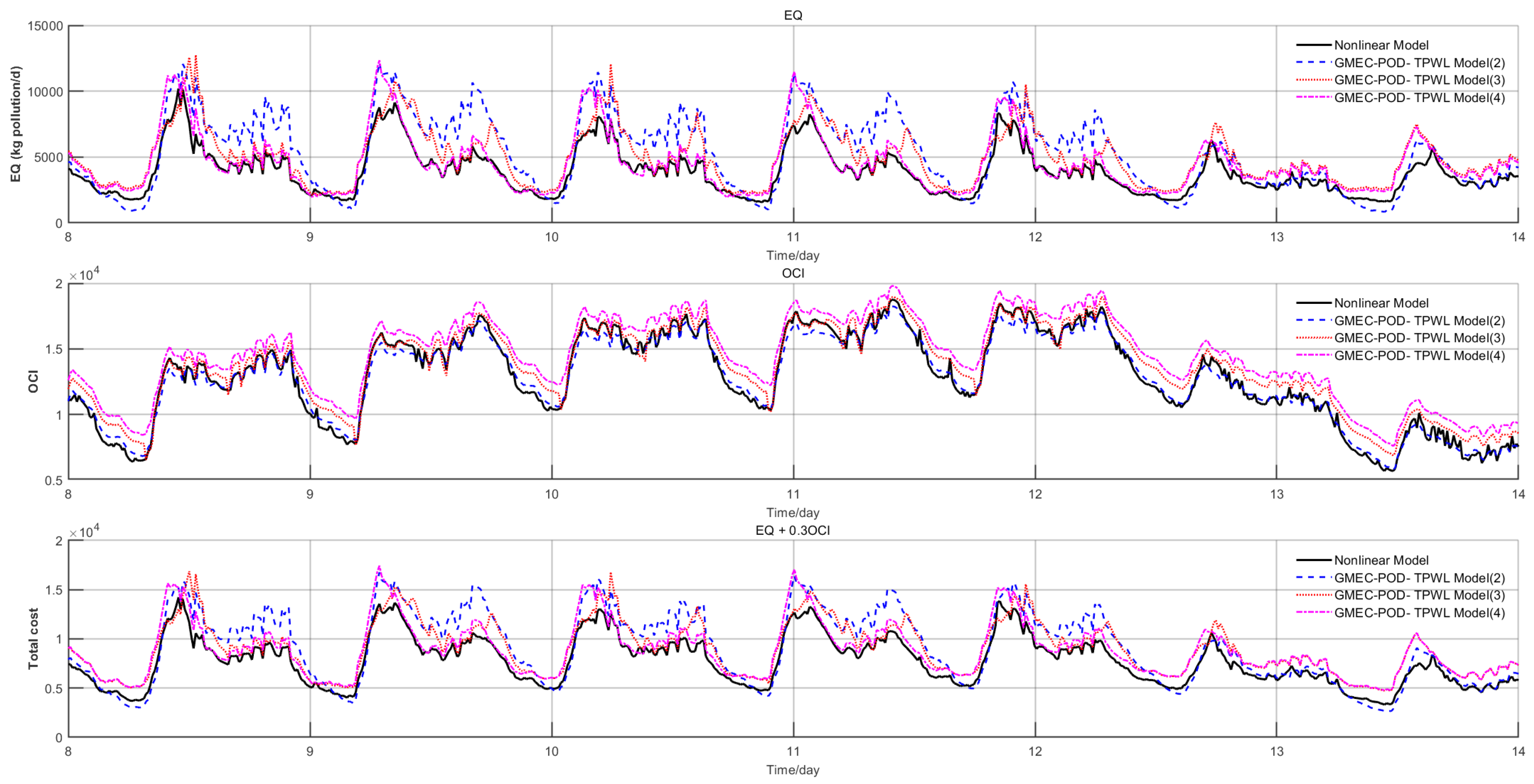
6.4. EMPC Simulation Performance Metrics Comparison
Under dry weather conditions, this study compares the EMPC control computation time, effluent quality (EQ), overall cost index (OCI), and economic cost index between the original model, the GMEC-POD-TPWL model, and the TPWL-POD model under varying numbers of linearization points. The results are summarized in
Table 5 and illustrated in the figures below.
Figure 6 displays the performance metric curves of the TPWL-POD model versus the original nonlinear model under different numbers of linearization points, while
Figure 7 shows the corresponding curves for the GMEC-POD-TPWL model. As specified in
Section 6.1, the comparison utilizes data from the last 7 days of the simulation period.
The experimental data demonstrate that both reduced-order models (TPWL-POD and GMEC-POD-TPWL) exhibit enhanced computational efficiency compared with the original nonlinear model. Specifically, increasing the number of linearization points improves model accuracy and control performance metrics for both approaches. The GMEC method ensures model accuracy through the implementation of a maximum error threshold, with its iterative process employing a maximum error prioritization strategy. Specifically, each iteration prioritizes the addition of linearization points that maximally reduce the peak approximation error in the simplified model, thereby guaranteeing progressive improvement in model fidelity. In contrast to conventional TPWL-POD approaches, which lack targeted error reduction mechanisms in their linearization point selection process and rely on increasing linearization point quantities to enhance accuracy—the GMEC-enhanced framework achieves superior model fidelity compared with conventional TPWL-POD implementations with equivalent numbers of linearization points. This accuracy advantage directly translates to enhanced EMPC control performance, as the refined model better preserves the dynamic characteristics of the original nonlinear system.
For the 4-linearization-point configuration, the GMEC-POD-TPWL model reduces computational time by 65.45% relative to the original nonlinear model (from
to
), though this acceleration introduces performance trade-offs: effluent quality (EQ) decreases by 18.56% (from
to
), while the overall cost index (OCI) and economic cost index increase by 13.19% and 15.88%, respectively. Compared with the TPWL-POD model [
13], the proposed method achieves a 2.28% faster computation speed (from
to
), coupled with a 44.34% reduction in model approximation error (from
to
). Furthermore, it demonstrates superior control performance, evidenced by an 11.40% lower effluent pollutant concentration and a 5.36% reduction in economic costs, despite a marginal 1.97% increase in OCI.
The experimental results demonstrate conclusively that the GMEC-POD-TPWL framework provides statistically significant improvements in model accuracy, effluent quality regulation, and economic cost optimization compared with existing TPWL-POD methodologies.


