Preview-Based Optimal Control for Trajectory Tracking of Fully-Actuated Marine Vessels

Abstract

In this paper, the problem of preview optimal control for second-order nonlinear systems for marine vessels is discussed on a fully actuated dynamic model. First, starting from a kinematic and dynamic model of a three-degrees-of-freedom (DOF) marine vessel, we derive a fully actuated second-order dynamic model that involves only the ship’s position and yaw angle. Subsequently, through the higher-order systems methodology, the nonlinear terms in the system were eliminated, transforming the system into a one-order parameterized linear system. Next, we designed an internal model compensator for the reference signal and constructed a new augmented error system based on this compensator. Then, using optimal control theory, we designed the optimal preview controller for the parameterized linear system and the corresponding feedback parameter matrices, which led to the preview controller for the original second-order nonlinear system. Finally, a numerical simulation indicates that the controller designed in this paper is highly effective.

1. Introduction

The advent and rapid evolution of autonomous maritime vehicles, particularly unmanned surface vessels (USVs), marks a pivotal shift in naval architecture and maritime operations. Their development is propelled by the pressing need for safer, more efficient, and cost-effective solutions to maritime challenges, ranging from environmental monitoring and oceanographic research to military surveillance and cargo transport. In the cutting-edge domain of maritime automation, trajectory tracking control methodologies for USVs represent a critical research focus [1,2,3]. These methods are vital to ensure that USVs can accurately follow predetermined paths through the complex and often unpreviewable marine environment. As the deployment of USVs expands across a myriad of applications—from oceanographic research and environmental monitoring to defense and commercial shipping—developing robust and reliable trajectory-tracking control techniques becomes imperative [4]. These control strategies must not only address the challenges posed by dynamic ocean currents, wind, and waves, but also navigate regulatory and safety considerations in increasingly crowded maritime spaces [5]. The essence of trajectory tracking control lies in its ability to integrate sophisticated algorithms, thereby enabling USVs to perform with unprecedented precision and autonomy. A detailed exploration delves into trajectory tracking control methods, uncovering their foundational principles and the technological innovations driving their advancement.

Preview control is a control method that can make reasonable use of information in advance to improve the effectiveness of system operation [6]. It was proposed in 1966 by Sheridan [7]. A proportional integral derivative plus preview controller (PIDP) was derived based on the linear quadratic optimal control theory by Tomizuka in 1979 [8]. After that, the augmented error system method was applied to the preview control problem, and the discrete- and continuous-time optimal preview controllers were obtained by Katayama in 1985 [9] and in 1987 [10]. On this basis, PIDP has also been applied to other dynamic systems, such as multirate setting systems [11,12], descriptor systems [13], and stochastic systems [14]. Preview control theory is also combined with other control methods, such as robust control [15,16], sliding mode control [17,18], repetitive control [19] and so on. Although these control methods are simple to implement, they do not allow for a direct extension to marine vessels since existing methods are more suitable for dealing with linear models. In order to improve the performance of marine vessels and improve the use of control resources, this paper proposes the use of high-order system approaches for the design of preview controllers for marine vessels.

In recent years, the advent of USVs has revolutionized the maritime industry. These cutting-edge vessels promise to redefine maritime operations, offering unparalleled benefits in terms of efficiency, safety, and cost-effectiveness [20]. However, the deployment of USVs introduces complex challenges, notably in navigating dynamic and often unpreviewable marine environments while ensuring safety and compliance with international maritime regulations. In this context, the application of optimal control emerges as a pivotal technological advancement [21,22].

The optimal preview control provides a robust mathematical framework for enforcing safety constraints in dynamic systems, making them invaluable tools for the autonomous navigation and control of unmanned ships. By integrating the optimal preview control into the fully actuated control systems of USVs, it is possible to systematically ensure that these vessels not only maintain safe distances from obstacles and other vessels but also adhere to navigational rules and environmental considerations [23]. This integration not only enhances the operational safety of USVs, but also paves the way for their wider acceptance and integration into the global maritime traffic system. Through this lens, our discussion explores the transformative impact of optimal preview control on the development and deployment of autonomous marine vessels, highlighting the potential for significant advancements in maritime safety, efficiency, and sustainability.

The main contributions are listed below.

(i)

This paper introduces a novel parametric design method that eliminates the nonlinear terms in a fully actuated second-order nonlinear marine vessel dynamic model, transforming it into a linear steady-state form. Compared to existing control methods [24,25,26], our approach retains the original nonlinear system’s dynamic characteristics while significantly simplifying the control design, enabling more precise control in variable dynamic models.

(ii)

An internal model is employed to construct a new augmented error system. We uniquely combine an internal model compensator with the error system approach to track reference signals with known structures. Unlike traditional optimal control methods that often fail to handle dynamic and variable reference trajectories efficiently [27], our compensator design enables robust tracking under complex dynamic environments. Furthermore, we rigorously derive stabilization and observability conditions to ensure system stability and control feasibility, setting this study apart from methods lacking theoretical guarantees.

(iii)

The paper presents a first application of optimization-based preview control, applied for fully actuated marine vessels. This approach focuses on state design, demonstrating its effectiveness through numerical simulations that validate the controller’s precision in trajectory tracking.

The remaining part of the paper is organized as follows. The technical preliminaries, and the problem formulation are demonstrated in Section 2. In Section 3, utilizing the methodology of preview control, a preview tracking controller with noteworthy and improved performance is designed for the trajectory tracking system. Here, the properties of both controllability and observability are rigorously established with optimal design conditions. Simulation results are conducted in Section 4, and Section 5 concludes this paper.

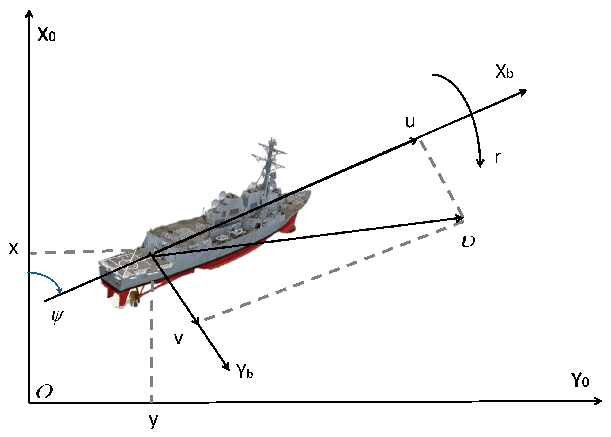
2. Problem Statement

The kinematic and kinetic of three DOF marine vessels in the earth-fixed and body-fixed coordinate frame are expressed as

$$\left\{\begin{array}{cc}\hfill \dot{\mathit{\eta }}& =\mathit{R}\left(\phi \right)\mathit{v},\hfill \\ \hfill \dot{\mathit{v}}& ={\mathit{M}}^{-1}(-\mathit{C}\left(\mathit{v}\right)\mathit{v}-\mathit{D}\left(\mathit{v}\right)\mathit{v}+\mathit{\tau }).\hfill \end{array}\right.$$

(1)

where $\mathit{\eta }={[{\eta }_x,{\eta }_y,\phi ]}^T$ is the position $({\eta }_x,{\eta }_y)$ and yaw angle $\phi$, $\mathit{v}={[u,\nu ,r]}^T$ is the surge velocity u, sway velocity $\nu$, and yaw rate r, $\mathit{\tau }={[{\tau }_1,{\tau }_2,{\tau }_3]}^T$ is the control input vector consisting of the surge force ${\tau }_1$, the sway force ${\tau }_2$, and the yaw torque ${\tau }_3$. Figure 1 describes the corresponding target model. The rotation matrix $\mathit{R}\left(\phi \right)$, the diagonal inertia matrix $\mathit{M}$, the Coriolis and centripetal matrix $\mathit{C}\left(\mathit{v}\right)$, and the damping matrix $\mathit{D}\left(\mathit{v}\right)$ can be given as follows:

$$\mathit{R}\left(\phi \right)=\left[\begin{array}{ccc}cos\phi & -sin\phi & 0\\ sin\phi & cos\phi & 0\\ 0& 0& 1\end{array}\right]$$

$$\mathit{M}=\left[\begin{array}{ccc}m-X_{\dot{u}}& 0& 0\\ 0& m-Y_{\dot{\nu }}& m{x}_g-Y_{\dot{r}}\\ 0& m{x}_g-Y_{\dot{r}}& I_z-N_{\dot{r}}\end{array}\right]$$

$$\mathit{C}\left(\mathit{v}\right)=\left[\begin{array}{ccc}0& 0& -(m-Y_{\dot{\nu }})\nu -(m{x}_g-Y_{\dot{r}})r\\ 0& 0& (m-X_{\dot{u}})u\\ (m-Y_{\dot{\nu }})\nu +(m{x}_g-Y_{\dot{r}})r& -(m-X_{\dot{u}})u& 0\end{array}\right]$$

$$\mathit{D}\left(\mathit{v}\right)=\left[\begin{array}{ccc}-X_u-X_{\left|u\right|u}\left|u\right|& 0& 0\\ 0& -Y_{\nu }-Y_{\left|\nu \right|\nu }\left|\nu \right|-Y_{\left|r\right|\nu }\left|r\right|\left(v\right)& -N_{\nu }-N_{\mid \nu |\nu }\left|\nu \right|-N_{\left|r\right|\nu }\left|r\right|\left(v\right)\\ 0& -Y_r-Y_{\left|\nu \right|r}\left|\nu \right|-Y_{\left|r\right|r}\left|r\right|& -N_r-N_{\left|\nu \right|r}\left|\nu \right|-N_{\left|r\right|r}\left|r\right|\}\left(v\right)\end{array}\right]$$

Here, m is the mass of the ship, $I_z$ is the moment of inertia about the yaw rotation, $x_g$ is the distance from the origin of the body-fixed frame to the center of gravity of the ship, the other symbols $X_{*}$, $Y_{*}$, $N_{*}$ are the corresponding hydrodynamic derivatives, and $Y_{\dot{r}}=N_{\dot{\nu }}$. In addition, $\mathit{M}$ is a positive definite matrix. It is noted that ${\mathit{R}}^T\left(\phi \right)\mathit{R}\left(\phi \right)=I$.

The generalized velocity $\mathit{v}$ is explicitly contained in the model (1). For navigation control, it is usually necessary to convert it into an explicit function containing only the generalized position $\eta$. Derivating the kinematic of system (1) with respect to t yields

$$\ddot{\mathit{\eta }}=\dot{\mathit{R}}\left(\phi \right)\mathit{v}+\mathit{R}\left(\phi \right)\dot{\mathit{v}}$$

(2)

where $\dot{\mathit{R}}\left(\phi \right)$ represents the total derivative of $\mathit{R}\left(\phi \right)$ with respect to t, i.e., $\dot{\mathit{R}}\left(\phi \right)={\displaystyle \frac{\mathrm{d}\mathit{R}\left(\phi \right)}{\mathrm{d}\phi }}{\displaystyle \frac{\mathrm{d}\phi }{\mathrm{d}t}}$. For convenience, it is abbreviated as $\dot{\mathit{R}}\left(\phi \right)$. It is obtained from (2) that $\dot{\mathit{v}}={\mathit{R}}^{-\mathbf{1}}\left(\phi \right)(\ddot{\mathit{\eta }}-\dot{\mathit{R}}\left(\phi \right)\mathit{v})$. Then, by substituting it into the dynamic equations of system (1), we derive

$$\mathit{M}{\mathit{R}}^{-\mathbf{1}}\left(\phi \right)\ddot{\mathit{\eta }}+\left[\mathit{C}\left(\mathit{v}\right)-\mathit{M}{\mathit{R}}^{-\mathbf{1}}\left(\phi \right)\dot{\mathit{R}}\left(\phi \right)\right]\mathit{v}+\mathit{D}\left(\mathit{v}\right)\mathit{v}=\mathit{\tau }$$

(3)

Furthermore, by utilizing $\mathit{v}={\mathit{R}}^{-\mathbf{1}}\left(\phi \right)\dot{\mathit{\eta }}$, and denoting ${\mathit{M}}_{\mathbf{0}}\left(\mathit{\eta }\right)=\mathit{M}{\mathit{R}}^{-\mathbf{1}}\left(\phi \right)$, ${\mathit{C}}_{\mathbf{0}}(\mathit{\eta },\dot{\mathit{\eta }})=\left[\mathit{C}\left(\mathit{v}\right)-\mathit{M}{\mathit{R}}^{-\mathbf{1}}\left(\phi \right)\dot{\mathit{R}}\left(\phi \right)\right]{\mathit{R}}^{-\mathbf{1}}\left(\phi \right)$, ${\mathit{D}}_{\mathbf{0}}(\mathit{\eta },\dot{\mathit{\eta }})=\mathit{D}\left(\mathit{v}\right){\mathit{R}}^{-\mathbf{1}}\left(\phi \right)$, one can acquire the following Euler–Lagrange system as

$${\mathit{M}}_{\mathbf{0}}\left(\mathit{\eta }\right)\ddot{\mathit{\eta }}+{\mathit{C}}_{\mathbf{0}}(\mathit{\eta },\dot{\mathit{\eta }})\dot{\mathit{\eta }}+{\mathit{D}}_{\mathbf{0}}(\mathit{\eta },\dot{\mathit{\eta }})\dot{\mathit{\eta }}=\mathit{\tau }$$

(4)

Let us consider the case that the design objective is to let the output $\mathit{\eta }$ track a properly given signal vector ${\eta }_d={[{\eta }_{xd},{\eta }_{yd},{\phi }_d]}^T$ generated by the following reference model:

$$\left\{\begin{array}{c}{\dot{\mathit{x}}}_{\mathit{d}}={\mathit{A}}_{\mathit{d}}{\mathit{x}}_{\mathit{d}}\hfill \\ {\eta }_{\mathit{d}}={\mathit{C}}_{\mathit{d}}{\mathit{x}}_{\mathit{d}}\hfill \end{array}\right.$$

(5)

where ${\mathit{A}}_{\mathit{d}}$ and ${\mathit{C}}_{\mathit{d}}$ are known constant matrices of appropriate dimensions.

Remark 1.

According to [28], if a reference trajectory ${\eta }_d\left(t\right)$ is given, we can establish the structural characteristics model of $y_d\left(t\right)$ based on system (5). Representing ${\eta }_d\left(t\right)$ in vector form gives:

$$\begin{array}{c}\hfill {\eta }_d\left(t\right)=\left[\begin{array}{c}{y}_{d1}\left(t\right)\\ y_{d2}\left(t\right)\\ ⋮\\ y_{dm}\left(t\right)\end{array}\right].\end{array}$$

(6)

Taking the Laplace transform of ${\eta }_d\left(t\right)$, we obtain:

$$\begin{array}{c}\hfill Y_d\left(s\right)=\left[\begin{array}{c}{\displaystyle \frac{n_1\left(s\right)}{p_1\left(s\right)}}\\ {\displaystyle \frac{n_2\left(s\right)}{p_2\left(s\right)}}\\ ⋮\\ {\displaystyle \frac{n_m\left(s\right)}{p_m\left(s\right)}}\end{array}\right].\end{array}$$

(7)

Here, $p\left(s\right)$ is referred to as the structural characteristic of ${\eta }_d\left(t\right)$, where $p\left(s\right)$ is the least common multiple of $p_1\left(s\right),p_2\left(s\right),\dots ,p_m\left(s\right)$. Moreover, $p\left(s\right)$ satisfies the following polynomial form:

$$\begin{array}{c}\hfill p\left(s\right)=s^r+{\alpha }_{r-1}{s}^{r-1}+\cdots +{\alpha }_{1}s+{\alpha }_0.\end{array}$$

(8)

Using Equations (7) and (8), system (5) can be derived. The least common multiple $p\left(s\right)$ forms the output of system (5).

In addition, the reference signal ${\eta }_{\mathit{d}}$ is satisfied the following assumption:

Assumption 1. The reference signals ${\eta }_{\mathit{d}}$ are piecewise continuous differentiable. ${\eta }_{\mathit{d}}$ is known for $t\le s\le t+l_r$, where $l_r$ is the preview length.

The control objective in this paper is to design a tracking controller $\mathit{\tau }$ with preview compensation for system (4) (i.e., (1)) by making full use of the previewable information of the reference signal ${\eta }_{\mathit{d}}$, so that the output vector can track the reference signal asymptotically.

Due to the limited research on preview controllers for nonlinear systems, most conclusions are based on first-order linear systems. However, the model (4) studied in this paper is a higher-order nonlinear one; therefore, we need to transform it formally.

First, for the system (4), by multiplying ${\mathit{M}}_{\mathbf{0}}^{-\mathbf{1}}\left(\mathit{\eta }\right)$ on both sides, we can obtain

$$\ddot{\mathit{\eta }}+{\mathit{M}}_{\mathbf{0}}^{-\mathbf{1}}\left(\mathit{\eta }\right)[{\mathit{C}}_{\mathbf{0}}(\mathit{\eta },\dot{\mathit{\eta }})\dot{\mathit{\eta }}+{\mathit{D}}_{\mathbf{0}}(\mathit{\eta },\dot{\mathit{\eta }})\dot{\mathit{\eta }}]={\mathit{M}}_{\mathbf{0}}^{-\mathbf{1}}\left(\mathit{\eta }\right)\mathit{\tau }$$

(9)

Then, the following controller is introduced for the system (9).

$$\mathit{\tau }={\mathit{M}}_{\mathbf{0}}\left(\mathit{\eta }\right)\left[-{\mathit{A}}_{\mathbf{1}}\dot{\mathit{\eta }}-{\mathit{A}}_{\mathbf{0}}\mathit{\eta }+\overline{\mathit{u}}\right]+{\mathit{C}}_{\mathbf{0}}(\mathit{\eta },\dot{\eta })\dot{\mathit{\eta }}+{\mathit{D}}_{\mathbf{0}}(\mathit{\eta },\dot{\mathit{\eta }})\dot{\mathit{\eta }}$$

(10)

where ${\mathit{A}}_{\mathbf{0}}$ and ${\mathit{A}}_{\mathbf{1}}$ are the gain matrices to be determined, $\overline{\mathit{u}}$ is virtual input.

Thus, we can obtain a higher-order linear system in the form of

$$\ddot{\mathit{\eta }}+{\mathit{A}}_{\mathbf{1}}\dot{\mathit{\eta }}+{\mathit{A}}_{\mathbf{0}}\mathit{\eta }=\overline{\mathit{u}}$$

(11)

Further, by letting ${\mathit{x}}^{\mathit{T}}={\left[\begin{array}{cc}{\mathit{\eta }}^{\mathit{T}}& {\dot{\mathit{\eta }}}^{\mathit{T}}\end{array}\right]}^T$, $\mathit{y}=\mathit{\eta }$, ${\mathit{A}}_{\mathit{c}}=\left[\begin{array}{cc}\mathbf{0}& \mathit{I}\\ -{\mathit{A}}_{\mathbf{0}}& -{\mathit{A}}_{\mathbf{1}}\end{array}\right]$, ${\mathit{B}}_{\mathit{c}}=\left[\begin{array}{c}\mathbf{0}\\ \mathit{I}\end{array}\right]$, and ${\mathit{C}}_{\mathit{c}}=\left[\begin{array}{cc}\mathit{I}& \mathbf{0}\end{array}\right]$, Equation (11) can be transformed into the following first-order system form

$$\left\{\begin{array}{c}\dot{\mathit{x}}={\mathit{A}}_{\mathit{c}}\mathit{x}+{\mathit{B}}_{\mathit{c}}\overline{\mathit{u}}\hfill \\ \mathit{y}={\mathit{C}}_{\mathit{c}}\mathit{x}\hfill \end{array}\right.$$

(12)

Denoting ${\mathit{A}}_{\mathit{c}\mathbf{0}}=\left[\begin{array}{cc}\mathbf{0}& \mathit{I}\\ \mathbf{0}& \mathbf{0}\end{array}\right]$ and $\mathit{K}=\left[\begin{array}{cc}-{\mathit{A}}_{\mathbf{0}}& -{\mathit{A}}_{\mathbf{1}}\end{array}\right]$, it is noted that ${\mathit{A}}_{\mathit{c}}={\mathit{A}}_{\mathit{c}\mathbf{0}}+{\mathit{B}}_{\mathit{c}}\mathit{K}$ and Equation (12) can be expressed equivalently as

$$\left\{\begin{array}{c}\dot{\mathit{x}}={\mathit{A}}_{\mathit{c}\mathbf{0}}\mathit{x}+{\mathit{B}}_{\mathit{c}}\overline{\mathit{v}}\hfill \\ \mathit{y}={\mathit{C}}_{\mathit{c}}\mathit{x}\hfill \end{array}\right.$$

(13)

where $\overline{\mathit{v}}=\mathit{Kx}+\overline{\mathit{u}}$.

As a result, designing the control law $\mathit{\tau }$ for the higher-order nonlinear system (4) is equivalent to finding the state feedback gain matrix $\mathit{K}$ and virtual input $\overline{\mathit{u}}$ for system (13).

Remark 2.

This paper introduces a novel parametric design method that eliminates the nonlinear terms in a fully actuated second-order nonlinear marine vessel dynamic model, transforming it into a linear steady-state form. While traditional nonlinear control methods, such as backstepping [24], sliding mode control [25], or adaptive control [26], often require complex designs tailored to specific system dynamics, our approach simplifies the control problem by systematically linearizing the original system without sacrificing its key dynamic characteristics. This contrasts with methods like backstepping, which can suffer from computational complexity and sensitivity to modeling errors, or sliding mode control, which may encounter chattering issues in practical applications. By achieving a linear representation, our method enables the application of advanced control strategies, such as optimization-based preview control, leading to significantly improved precision and robustness in complex marine environments. Furthermore, the proposed method maintains computational efficiency and facilitates theoretical analysis, offering a clear advantage over many traditional nonlinear techniques in terms of practicality and scalability.

3. Designing the Preview Tracking Control

Let the error signal $\mathit{e}$ as the difference between $\mathit{y}$ and ${\eta }_{\mathit{d}}$, i.e,

$$\mathit{e}=\mathit{y}-{\eta }_{\mathit{d}}$$

(14)

The concept of the internal model is used to construct an augmented system together with the technique of preview control. The definition of the minimal m-copy internal model is given beforehand. To illustrate an overview of the algorithm, the block diagram for the proposed control algorithm is shown in Figure 2.

Theorem 1.

Definition 1 [29]: Given any square matrix ${\mathit{A}}_{\mathit{d}}$, a pair of matrix $(\mathit{G}\mathbf{1},\mathit{G}\mathbf{2})$ is said to incorporate a minimal m-copy internal model of the matrix ${\mathit{A}}_{\mathit{d}}$, if the pair admits the following form:

$$G_1={\left[\begin{array}{cccc}\beta & 0& \cdots & 0\\ 0& \beta & \cdots & 0\\ ⋮& ⋮& \ddots & ⋮\\ 0& 0& \cdots & \beta \end{array}\right]}_{md\times md}$$

$$G_2={\left[\begin{array}{cccc}\theta & 0& \cdots & 0\\ 0& \theta & \cdots & 0\\ ⋮& ⋮& \ddots & ⋮\\ 0& 0& \cdots & \theta \end{array}\right]}_{md\times m}$$

where $\beta$ is a $d\times d$ constant square matrix and $\theta$ is a $d\times 1$ constant column vector, such that

1. 

$(\beta ,\theta )$ is controllable;

2. 

the characteristic polynomial of $\beta$, the minimal polynomial of $\beta$ and the minimal polynomial of ${\mathit{A}}_{\mathit{d}}$ are all the same.

Based on Definition 1, an internal model compensator is taken as

$$\dot{\mathit{\xi }}={\mathit{G}}_{\mathbf{1}}\mathit{\xi }+{\mathit{G}}_{\mathbf{2}}\mathit{e}$$

(15)

Differentiating both sides of (14) with respect to t and utilizing system (13) gives

$$\dot{\mathit{e}}={\mathit{C}}_{\mathit{c}}\dot{\mathit{x}}-{\dot{\mathit{\eta }}}_{\mathit{d}}$$

(16)

Introducing ${\overline{\mathit{x}}}^{\mathit{T}}={\left[\begin{array}{ccc}{\dot{\mathit{x}}}^{\mathit{T}}& {\mathit{\xi }}^{\mathit{T}}& {\mathit{e}}^{\mathit{T}}\end{array}\right]}^T$ and combining Equations (13), (15) and (16), the following dynamic equation is acquired:

$$\dot{\overline{\mathit{x}}}=\overline{\mathit{A}}\overline{\mathit{x}}+\overline{\mathit{B}}\dot{\overline{\mathit{v}}}+\overline{\mathit{D}}{\dot{\mathit{\eta }}}_{\mathit{d}}$$

(17)

where $\overline{\mathit{A}}=\left[\begin{array}{ccc}{\mathit{A}}_{\mathit{c}\mathbf{0}}& \mathbf{0}& \mathbf{0}\\ \mathbf{0}& {\mathit{G}}_{\mathbf{1}}& {\mathit{G}}_{\mathbf{2}}\\ {\mathit{C}}_{\mathit{c}}& \mathbf{0}& \mathbf{0}\end{array}\right]$, $\overline{\mathit{B}}=\left[\begin{array}{c}{\mathit{B}}_{\mathit{c}}\\ \mathbf{0}\\ \mathbf{0}\end{array}\right]$, $\overline{\mathit{D}}=\left[\begin{array}{c}\mathbf{0}\\ \mathbf{0}\\ -\mathit{I}\end{array}\right]$.

Similar to [9], we take the observation equation as

$$\mathit{e}=\overline{\mathit{C}}\overline{\mathit{x}}$$

(18)

where $\overline{\mathit{C}}=\left[\begin{array}{ccc}\mathbf{0}& \mathbf{0}& \mathit{I}\end{array}\right]$.

By combining Equations (17) and (18), the following augmented system is obtained.

$$\left\{\begin{array}{c}\dot{\overline{\mathit{x}}}=\overline{\mathit{A}}\overline{\mathit{x}}+\overline{\mathit{B}}\dot{\overline{\mathit{v}}}+\overline{\mathit{D}}{\dot{\mathit{\eta }}}_{\mathit{d}}\hfill \\ \mathit{e}=\overline{\mathit{C}}\overline{\mathit{x}}\hfill \end{array}\right.$$

(19)

To evaluate the tracking quality, we introduce the following cost function

$$J={\displaystyle \frac{1}{2}}{\int }_0^{\infty }\left[{\overline{\mathit{x}}}^{\mathit{T}}\mathit{Q}\overline{\mathit{x}}+{\dot{\overline{\mathit{v}}}}^{\mathit{T}}\mathit{R}\dot{\overline{\mathit{v}}}\right]\mathrm{d}t$$

(20)

where $\mathit{Q}=\left[\begin{array}{ccc}\mathbf{0}& \mathbf{0}& \mathbf{0}\\ \mathbf{0}& {\mathit{Q}}_{\xi }& \mathbf{0}\\ \mathbf{0}& \mathbf{0}& {\mathit{Q}}_{\mathit{e}}\end{array}\right]$, and ${\mathit{Q}}_{\mathit{\xi }}$, ${\mathit{Q}}_{\mathit{e}}$ and $\mathit{R}$ are positive definite matrices.

Let ${\mathit{Q}}_{\mathit{e}}={\mathit{C}}_{\mathit{e}}^{\mathit{T}}{\mathit{C}}_{\mathit{e}}$, ${\mathit{Q}}_{\mathit{\xi }}={\mathit{C}}_{\mathit{\xi }}^{\mathit{T}}{\mathit{C}}_{\mathit{\xi }}$, then we have $\mathit{Q}={\overline{\mathit{C}}}^{\mathit{T}}\overline{\mathit{C}}$, where ${\mathit{Q}}^{\mathbf{1}/\mathbf{2}}=\overline{\mathit{C}}=\left[\begin{array}{ccc}\mathbf{0}& \mathbf{0}& \mathbf{0}\\ \mathbf{0}& {\mathit{C}}_{\mathit{\xi }}& \mathbf{0}\\ \mathbf{0}& \mathbf{0}& {\mathit{C}}_{\mathit{e}}\end{array}\right].$

By employing the results of [10,12], the following theorem can immediately hold.

Lemma 1.

Suppose that $(\overline{\mathit{A}},\overline{\mathit{B}})$ is stabilizable and $({\mathit{Q}}^{\mathbf{1}/\mathbf{2}},\overline{\mathit{A}})$ is detectable, then the optimal control input of system (19) that minimizes quadratic performance index (20) is

$$\dot{\overline{\mathit{v}}}=-{\mathit{R}}^{-\mathbf{1}}{\overline{\mathit{B}}}^{\mathit{T}}\mathit{P}\overline{\mathit{x}}-{\mathit{R}}^{-\mathbf{1}}{\overline{\mathit{B}}}^{\mathit{T}}\mathit{z}$$

(21)

where $\mathit{P}$ is a positive semi-definite matrix satisfying the algebraic Riccati equation

$${\overline{\mathit{A}}}^{\mathit{T}}\mathit{P}+\mathit{P}\overline{\mathit{A}}-\mathit{P}\overline{\mathit{B}}{\mathit{R}}^{-\mathbf{1}}{\overline{\mathit{B}}}^{\mathit{T}}\mathit{P}+\mathit{Q}=\mathbf{0}$$

(22)

and $\mathit{z}$ is determined as follows:

$$\mathit{z}={\int }_0^{l_r}exp\left(\sigma {\overline{\mathit{A}}}_{\mathit{c}}^{\mathit{T}}\right)\mathit{P}\overline{\mathit{D}}{\dot{\mathit{\eta }}}_{\mathit{d}}(t+\sigma )\mathrm{d}\sigma$$

(23)

with ${\overline{\mathit{A}}}_{\mathit{c}}=\overline{\mathit{A}}-\overline{\mathit{B}}{\mathit{R}}^{-\mathbf{1}}{\overline{\mathit{B}}}^{\mathit{T}}\mathit{P}$.

Proof. 

The proof is elementary and is referred to [10,12]. □

In order to ensure the existence of $\overline{\mathit{v}}$, we need to derive the conditions that ensure $(\overline{\mathit{A}},\overline{\mathit{B}})$ can be stabilized and $({\mathit{Q}}^{\mathbf{1}/\mathbf{2}},\overline{\mathit{A}})$ can be detected. For this purpose, we derive the following lemmas.

Lemma 2.

The pair $(\overline{\mathit{A}},\overline{\mathit{B}})$ is stabilizable if and only if the pair $({\mathit{G}}_{\mathbf{1}},{\mathit{G}}_{\mathbf{2}})$ is stabilizable.

Proof. 

Let ${\mathbb{C}}^{+}$ denote the right half-plane of the complex plane. If $(\overline{\mathit{A}},\overline{\mathit{B}})$ can be stabilized, then for any $s\in {\mathbb{C}}^{+}$, we have

$$\begin{array}{c}\left[\begin{array}{cc}\overline{\mathit{A}}-s\mathit{I}& \overline{\mathit{B}}\end{array}\right]\begin{array}{c}\hfill =\left[\begin{array}{cccc}{\mathit{A}}_{\mathit{c}\mathbf{0}}-s\mathit{I}& \mathbf{0}& \mathbf{0}& {\mathit{B}}_{\mathit{c}}\\ \mathbf{0}& {\mathit{G}}_{\mathbf{1}}-s\mathit{I}& {\mathit{G}}_{\mathbf{2}}& \mathbf{0}\\ {\mathit{C}}_{\mathit{c}}& \mathbf{0}& \mathbf{0}-s\mathit{I}& \mathbf{0}\end{array}\right].\end{array}\hfill \end{array}$$

(24)

Substituting ${\mathit{A}}_{\mathit{c}\mathbf{0}}=\left[\begin{array}{cc}\mathbf{0}& \mathit{I}\\ \mathbf{0}& \mathbf{0}\end{array}\right]$, ${\mathit{B}}_{\mathit{c}}=\left[\begin{array}{c}\mathbf{0}\\ \mathit{I}\end{array}\right]$ and ${\mathit{C}}_{\mathit{c}}=\left[\begin{array}{cc}\mathit{I}& \mathbf{0}\end{array}\right]$ into (24), we obtain

$$\begin{array}{c}\mathrm{rank}\left[\begin{array}{cc}\overline{\mathit{A}}-s\mathit{I}& \overline{\mathit{B}}\end{array}\right]\hfill \\ \begin{array}{c}\hfill =\mathrm{rank}\left[\begin{array}{ccccc}\mathbf{0}-s\mathit{I}& \mathit{I}& \mathbf{0}& \mathbf{0}& \mathbf{0}\\ \mathbf{0}& \mathbf{0}-s\mathit{I}& \mathbf{0}& \mathbf{0}& \mathit{I}\\ \mathbf{0}& \mathbf{0}& {\mathit{G}}_{\mathbf{1}}-s\mathit{I}& {\mathit{G}}_{\mathbf{2}}& \mathbf{0}\\ \mathit{I}& \mathbf{0}& \mathbf{0}& \mathbf{0}-s\mathit{I}& \mathbf{0}\end{array}\right]=9+md(\mathrm{full}\mathrm{row}\mathrm{rank}),\end{array}\hfill \end{array}$$

(25)

which implies that the pair $({\mathit{G}}_{\mathbf{1}},{\mathit{G}}_{\mathbf{2}})$ is stabilizable, if and only if the pair $(\overline{\mathit{A}},\overline{\mathit{B}})$ is stabilizable. □

Lemma 3.

If ${\mathit{Q}}_{\mathit{e}}$ and ${\mathit{Q}}_{\mathit{\xi }}$ are positive-definite, then the pair $({\mathit{Q}}^{\mathbf{1}/\mathbf{2}},\overline{\mathit{A}})$ is detectable.

Proof. 

For any $s\in {\mathbb{C}}^{+}$, we have

$$\begin{array}{c}\left[\begin{array}{c}\overline{\mathit{C}}\\ \overline{\mathit{A}}-s\mathit{I}\end{array}\right]\begin{array}{c}\hfill =\left[\begin{array}{ccc}\mathbf{0}& \mathbf{0}& \mathbf{0}\\ \mathbf{0}& {\mathit{C}}_{\mathit{\xi }}& \mathbf{0}\\ \mathbf{0}& \mathbf{0}& {\mathit{C}}_{\mathit{e}}\\ {\mathit{A}}_{\mathit{c}\mathbf{0}}-s\mathit{I}& \mathbf{0}& \mathbf{0}\\ \mathbf{0}& {\mathit{G}}_{\mathbf{1}}-s\mathit{I}& {\mathit{G}}_{\mathbf{2}}\\ {\mathit{C}}_{\mathit{c}}& \mathbf{0}& \mathbf{0}-s\mathit{I}\end{array}\right].\end{array}\hfill \end{array}$$

(26)

Substituting ${\mathit{A}}_{\mathit{c}\mathbf{0}}=\left[\begin{array}{cc}\mathbf{0}& \mathit{I}\\ \mathbf{0}& \mathbf{0}\end{array}\right]$, ${\mathit{B}}_{\mathit{c}}=\left[\begin{array}{c}\mathbf{0}\\ \mathit{I}\end{array}\right]$ and ${\mathit{C}}_{\mathit{c}}=\left[\begin{array}{cc}\mathit{I}& \mathbf{0}\end{array}\right]$ into (26), we obtain

$$\begin{array}{c}\mathrm{rank}\left[\begin{array}{c}\overline{\mathit{C}}\\ \overline{\mathit{A}}-s\mathit{I}\end{array}\right]\begin{array}{c}\hfill =\mathrm{rank}\left[\begin{array}{cccc}\mathbf{0}& \mathbf{0}& \mathbf{0}& \mathbf{0}\\ \mathbf{0}& \mathbf{0}& \mathbf{0}& \mathbf{0}\\ \mathbf{0}& \mathbf{0}& {\mathit{C}}_{\mathit{\xi }}& \mathbf{0}\\ \mathbf{0}& \mathbf{0}& \mathbf{0}& {\mathit{C}}_{\mathit{e}}\\ \mathbf{0}-s\mathit{I}& \mathit{I}& \mathbf{0}& \mathbf{0}\\ \mathbf{0}& \mathbf{0}-s\mathit{I}& \mathbf{0}& \mathbf{0}\\ \mathbf{0}& \mathbf{0}& {\mathit{G}}_{\mathbf{1}}-s\mathit{I}& {\mathit{G}}_{\mathbf{2}}\\ \mathit{I}& \mathbf{0}& \mathbf{0}& \mathbf{0}-s\mathit{I}\end{array}\right],\end{array}\hfill \end{array}$$

(27)

which implies that the matrix is full column rank for any $s\in {\mathbb{C}}^{+}$ with ${\mathit{C}}_{\mathit{e}}$ and ${\mathit{C}}_{\mathit{\xi }}$ are positive-definite, i.e., ${\mathit{Q}}_{\mathit{e}}$ and ${\mathit{Q}}_{\mathit{\xi }}$ are positive-definite. Then $({\mathit{Q}}^{\mathbf{1}/\mathbf{2}},\overline{\mathit{A}})$ can be detectable. □

Remark 3.

Our study rigorously proves controllability, observability, and stabilizability under the augmented system framework. Unlike other studies that rely heavily on experimental or heuristic approaches [30], this paper provides a complete mathematical foundation, ensuring the robustness and universality of the proposed control strategy.

Let $\mathit{P}=\left[\begin{array}{ccc}{\mathit{P}}_{\mathit{x}}& {\mathit{P}}_{\mathit{\xi }}& {\mathit{P}}_{\mathit{e}}\end{array}\right]$. Thus, we obtain the optimal preview controller for the system (13) according to Theorem 2.

Theorem 2.

Suppose that $({\mathit{G}}_{\mathbf{1}},{\mathit{G}}_{\mathbf{2}})$ is stabilizable, and ${\mathit{Q}}_{\mathit{e}}$ and ${\mathit{Q}}_{\mathit{\xi }}$ are positive-definite, then the optimal control input of system (13) that minimizes quadratic performance index (20) is

$$\begin{array}{cc}\hfill \overline{\mathit{v}}\left(\mathit{t}\right)=& -{\mathit{R}}^{-\mathbf{1}}{\overline{\mathit{B}}}^{\mathit{T}}{\mathit{P}}_{\mathit{x}}\mathit{x}\left(t\right)\hfill \\ \hfill & -{\mathit{R}}^{-\mathbf{1}}{\overline{\mathit{B}}}^{\mathit{T}}{\int }_0^t{\mathit{P}}_{\mathit{\xi }}\mathit{\xi }\left(s\right)ds-{\mathit{R}}^{-\mathbf{1}}{\overline{\mathit{B}}}^{\mathit{T}}{\int }_0^t{\mathit{P}}_{\mathit{e}}\mathit{e}\left(s\right)ds\hfill \\ \hfill & -{\mathit{R}}^{-\mathbf{1}}{\overline{\mathit{B}}}^{\mathit{T}}{\int }_0^t{\int }_0^{l_r}exp\left(\sigma {\overline{\mathit{A}}}_{\mathit{c}}^{\mathit{T}}\right)\mathit{P}\overline{\mathit{D}}{\dot{\mathit{\eta }}}_{\mathit{d}}(s+\sigma )d\sigma ds.\hfill \end{array}$$

(28)

Proof. 

It is known from Lemmas 2 and 3 that under the conditions of this Theorem, Lemma 1 holds. The expression of $\dot{\overline{\mathit{v}}}\left(t\right)$ is given in Lemma 1 where $\mathit{P}=\left[\begin{array}{cccc}{\mathit{P}}_{\mathit{\eta }}& {\mathit{P}}_{\dot{\mathit{\eta }}}& {\mathit{P}}_{\mathit{\xi }}& {\mathit{P}}_{\mathit{e}}\end{array}\right]$.

Therefore we only need to solve for $\overline{\mathit{v}}\left(t\right)$ from Lemma 1, which $\overline{\mathit{v}}\left(t\right)$ is the optimal control input of system (13) that minimizes quadratic performance index (20). To do this, setting $\overline{\mathit{v}}\left(\mathbf{0}\right)=\mathbf{0}$ and $\mathit{x}\left(0\right)=0$, and then integrating both sides of (21) from 0 to t yields $\overline{\mathit{v}}\left(t\right)$ given by (28). This completes the proof of Theorem 1. □

Based on the discussion of the above theorem, we give the preview controller of systems (4).

Theorem 3.

Suppose that

• $({\mathit{G}}_{\mathbf{1}},{\mathit{G}}_{\mathbf{2}})$ is stabilizable;
• ${\mathit{Q}}_{\mathit{\xi }}$, ${\mathit{Q}}_{\mathit{e}}$ and $\mathit{R}$ are positive definite;
• the dynamical compensator (15) incorporates a minimal m-copy internal model of the matrix ${\mathit{A}}_{\mathit{d}}$,

then the preview tracking controller can be designed for the systems (4) as follows:

$$\mathit{\tau }={\mathit{M}}_{\mathbf{0}}\left(\mathit{\eta }\right)\left[-{\mathit{A}}_{\mathbf{1}}\dot{\mathit{\eta }}-{\mathit{A}}_{\mathbf{0}}\mathit{\eta }+\overline{\mathit{u}}\right]+{\mathit{C}}_{\mathbf{0}}(\mathit{\eta },\dot{\mathit{\eta }})\dot{\mathit{\eta }}+{\mathit{D}}_{\mathbf{0}}(\mathit{\eta },\dot{\mathit{\eta }})\dot{\mathit{\eta }}$$

(29)

where ${\mathit{A}}_{\mathbf{1}}={\mathit{R}}^{-\mathbf{1}}{\overline{\mathit{B}}}^{\mathit{T}}{\mathit{P}}_{\dot{\mathit{\eta }}}$, ${\mathit{A}}_{\mathbf{0}}={\mathit{R}}^{-\mathbf{1}}{\overline{\mathit{B}}}^{\mathit{T}}{\mathit{P}}_{\mathit{\eta }}$,

$$\overline{\mathit{u}}=-{\mathit{R}}^{-\mathbf{1}}{\overline{\mathit{B}}}^{\mathit{T}}{\int }_0^t{\mathit{P}}_{\mathit{\xi }}\mathit{\xi }\left(s\right)\mathrm{d}s-{\mathit{R}}^{-\mathbf{1}}{\overline{\mathit{B}}}^{\mathit{T}}{\int }_0^t{\mathit{P}}_{\mathit{e}}\mathit{e}\left(s\right)\mathrm{d}s-\mathit{g}\left(t\right),$$

(30)

$$\mathit{g}\left(t\right)={\mathit{R}}^{-\mathbf{1}}{\overline{\mathit{B}}}^{\mathit{T}}{\int }_0^t{\int }_0^{l_r}exp\left(\sigma {\overline{\mathit{A}}}_{\mathit{c}}^{\mathit{T}}\right)\mathit{P}\overline{\mathit{D}}{\mathit{C}}_{\mathit{d}}{\mathit{A}}_{\mathit{d}}\mathit{W}{\mathit{\eta }}_{\mathit{d}}(s+\sigma )\mathrm{d}\sigma \mathrm{d}s,$$

(31)

and $\mathit{W}={\mathit{C}}_{\mathit{d}}^{\mathit{T}}{\left({\mathit{C}}_{\mathit{d}}{\mathit{C}}_{\mathit{d}}^{\mathit{T}}\right)}^{-\mathbf{1}}$.

Proof. 

According to Theorem 2, (28) can serve as the preview controller for system (13). Due to ${\mathit{x}}^{\mathit{T}}={\left[\begin{array}{cc}{\mathit{\eta }}^{\mathit{T}}& {\dot{\mathit{\eta }}}^{\mathit{T}}\end{array}\right]}^T$, it is noticed that (28) can be expressed as

$$\begin{array}{cc}\hfill \overline{\mathit{v}}=& -{\mathit{R}}^{-1}{\overline{\mathit{B}}}^{\mathit{T}}{\mathit{P}}_{\eta }\mathit{\eta }-{\mathit{R}}^{-1}{\overline{\mathit{B}}}^{\mathit{T}}{\mathit{P}}_{\dot{\eta }}\dot{\mathit{\eta }}\hfill \\ \hfill & -{\mathit{R}}^{-\mathbf{1}}{\overline{\mathit{B}}}^{\mathit{T}}{\int }_0^t{\mathit{P}}_{\mathit{\xi }}\mathit{\xi }\left(s\right)\mathrm{d}s-{\mathit{R}}^{-\mathbf{1}}{\overline{\mathit{B}}}^{\mathit{T}}{\int }_0^t{\mathit{P}}_{\mathit{e}}\mathit{e}\left(s\right)\mathrm{d}s\hfill \\ \hfill & -{\mathit{R}}^{-\mathbf{1}}{\overline{\mathit{B}}}^{\mathit{T}}{\int }_0^t{\int }_0^{l_r}exp\left(\sigma {\overline{\mathit{A}}}_{\mathit{c}}^{\mathit{T}}\right)\mathit{P}\overline{\mathit{D}}{\dot{\mathit{\eta }}}_{\mathit{d}}(s+\sigma )\mathrm{d}\sigma \mathrm{d}s.\hfill \end{array}$$

(32)

On the other hand, designing the control law $\mathit{\tau }$ for the higher-order nonlinear system (4) is equivalent to finding the state feedback gain matrix $\mathit{K}$ and virtual input $\overline{\mathit{u}}$ for system (13).

Also, because $\overline{\mathit{v}}=\mathit{Kx}+\overline{\mathit{u}}$, one can obtain ${\mathit{A}}_{\mathbf{1}}={\mathit{R}}^{-\mathbf{1}}{\overline{\mathit{B}}}^{\mathit{T}}{\mathit{P}}_{\dot{\mathit{\eta }}}$, ${\mathit{A}}_{\mathbf{0}}={\mathit{R}}^{-\mathbf{1}}{\overline{\mathit{B}}}^{\mathit{T}}{\mathit{P}}_{\mathit{\eta }}$, and

$$\begin{array}{cc}\hfill \overline{\mathit{u}}\left(\mathit{t}\right)=& -{\mathit{R}}^{-\mathbf{1}}{\overline{\mathit{B}}}^{\mathit{T}}{\int }_0^t{\mathit{P}}_{\xi }\mathit{\xi }\left(s\right)\mathrm{d}s-{\mathit{R}}^{-\mathbf{1}}{\overline{\mathit{B}}}^{\mathit{T}}{\int }_0^t{\mathit{P}}_e\mathit{e}\left(s\right)\mathrm{d}s\hfill \\ \hfill & -{\mathit{R}}^{-\mathbf{1}}{\overline{\mathit{B}}}^{\mathit{T}}{\int }_0^t{\int }_0^{l_r}exp\left(\sigma {\overline{\mathit{A}}}_{\mathit{c}}^{\mathit{T}}\right)\mathit{P}\overline{\mathit{D}}{\dot{\mathit{\eta }}}_{\mathit{d}}(s+\sigma )\mathrm{d}\sigma \mathrm{d}s\hfill \end{array}$$

(33)

The gain matrix $\mathit{K}$ yields

$$\begin{array}{c}\hfill \mathit{K}=\left[\begin{array}{cc}-{\mathit{R}}^{-\mathbf{1}}{\overline{\mathit{B}}}^{\mathit{T}}{\mathit{P}}_{\mathit{\eta }}& -{\mathit{R}}^{-\mathbf{1}}{\overline{\mathit{B}}}^{\mathit{T}}{\mathit{P}}_{\dot{\mathit{\eta }}}\end{array}\right]\end{array}$$

(34)

In addition, based on (5), we have ${\dot{\mathit{\eta }}}_{\mathit{d}}={\mathit{C}}_{\mathit{d}}{\mathit{A}}_{\mathit{d}}{\mathit{x}}_{\mathit{d}}$ and ${\mathit{x}}_{\mathit{d}}={\mathit{C}}_{\mathit{d}}^{\mathit{T}}{\left({\mathit{C}}_{\mathit{d}}{\mathit{C}}_{\mathit{d}}^{\mathit{T}}\right)}^{-\mathbf{1}}{\mathit{\eta }}_{\mathit{d}}=\mathit{W}{\mathit{\eta }}_{\mathit{d}}$. Thus,

$${\dot{\mathit{\eta }}}_{\mathit{d}}={\mathit{C}}_{\mathit{d}}{\mathit{A}}_{\mathit{d}}\mathit{W}{\mathit{\eta }}_{\mathit{d}}$$

(35)

Substituting (35) into (33) immediately yields (30). To sum up, the proof for Theorem 3 is completed. □

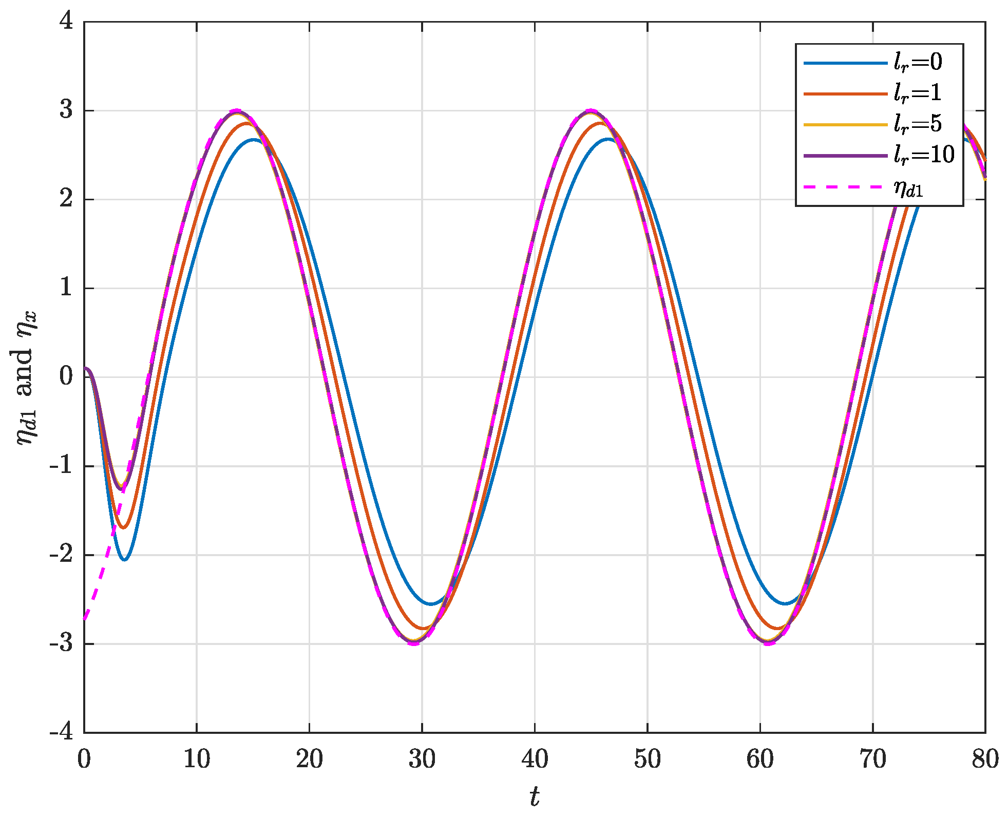
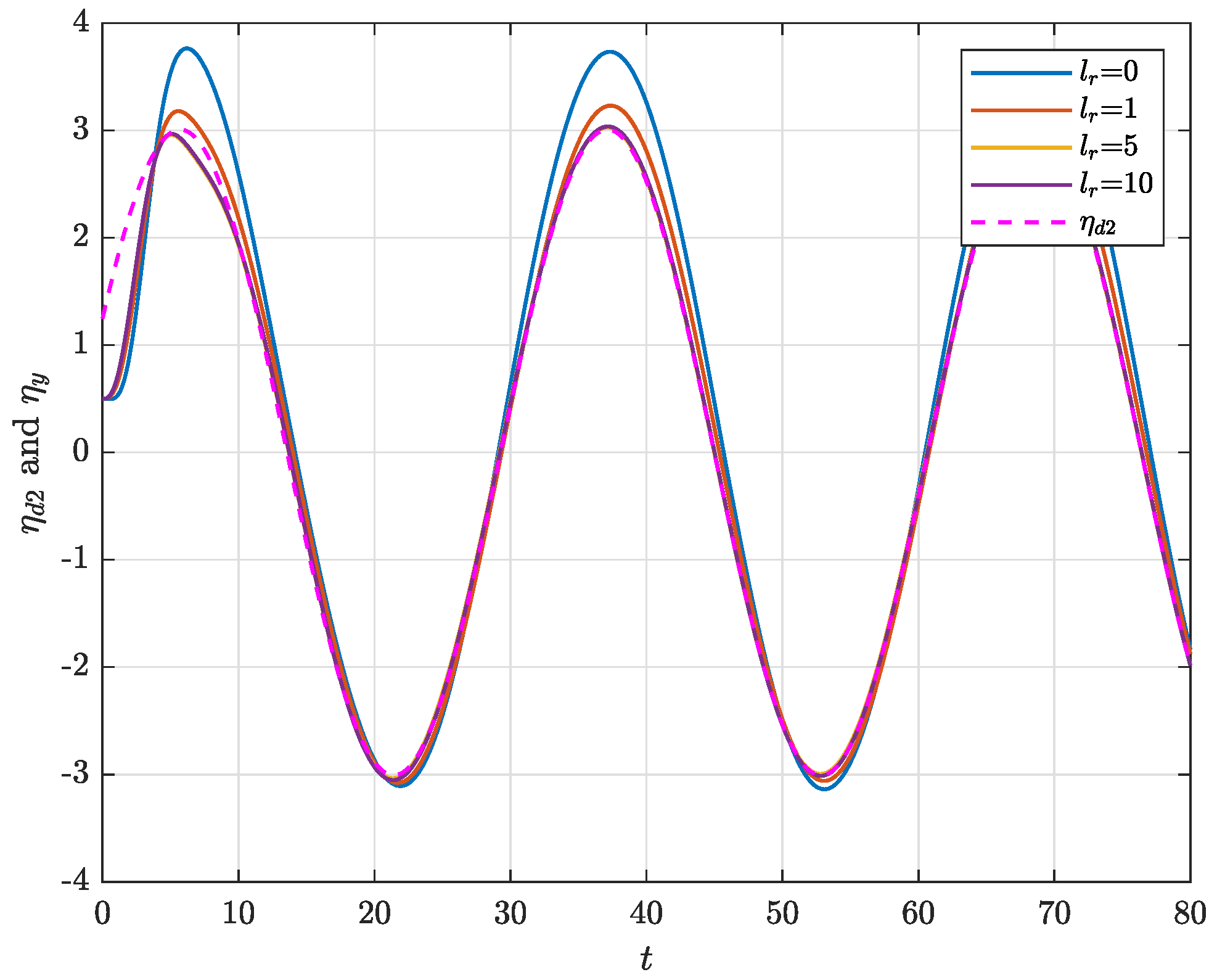
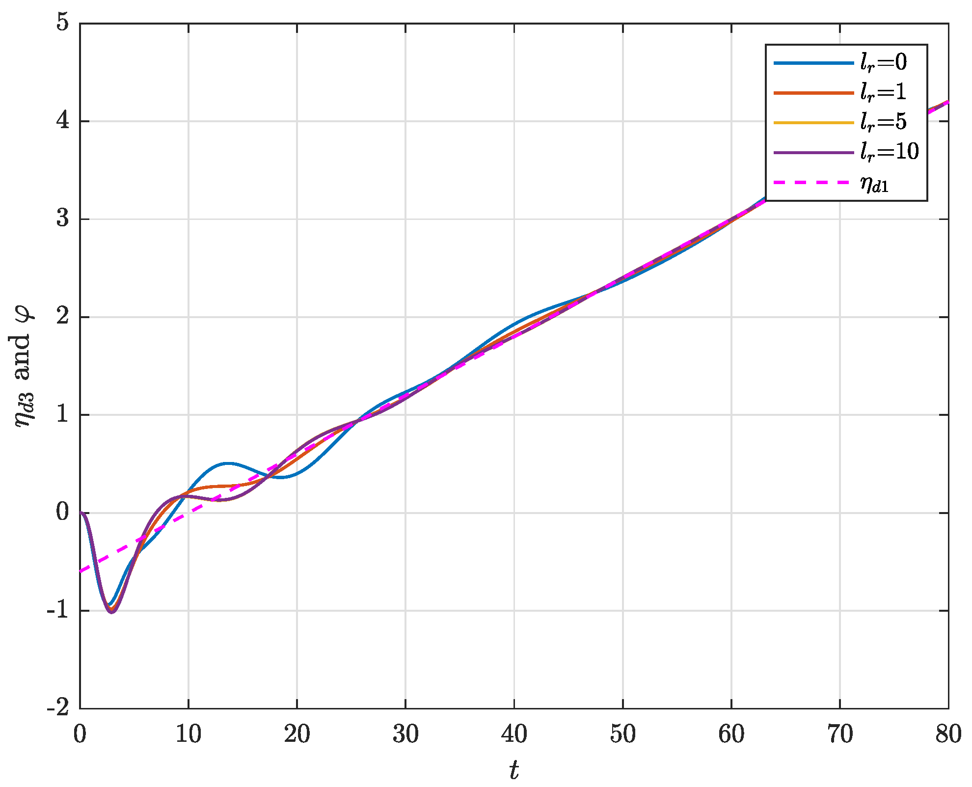
4. Illustrative Example

In this section, we conduct numerical simulations to validate the performance of the proposed preview-based optimal controller for a fully actuated second-order nonlinear marine vessel system. The dynamic model of the marine vessel is developed based on the well-known Cybership II model [31], which accurately represents the vessel’s kinematics and dynamics in three degrees of freedom (DOF). The

Table 1. Cybership II parameters [31].

Parameter	Symbol	Value
Mass of the ship	m	$23.8$ kg
Added mass in surge	$X_u$	$-0.7225$ kg
Added mass in sway	$Y_v$	$-0.8612$ kg
Added mass in yaw	$N_r$	$-0.96$ kg·m2
Hydrodynamic damping in surge	$X_{\dot{u}}$	$-2$ kg
Hydrodynamic damping in sway	$Y_{\dot{v}}$	$-10$ kg
Hydrodynamic damping in yaw	$N_{\dot{r}}$	$-1$ kg·m2
Length of the ship	L	$1.255$ m
Beam of the ship	B	$0.29$ m

lists key parameters for the Cybership II model, commonly used in marine vessel control simulations. The parameter column lists each physical quantity, such as mass, added mass, linear damping, and dimensions of the marine vessel. The symbol column gives the mathematical notation used for these parameters. The value column provides the specific numerical values associated with each parameter.

In actual ship navigation, steady-state motion can be regarded as trajectory tracking of a step signal, while uniformly accelerated motion corresponds to trajectory tracking of a ramp signal. To validate the ship’s steering performance, the reference signal is set as a sinusoidal or cosine signal. Simulations have been conducted for these three types of reference signals, and the entire physical process has been thoroughly explained.

We derive a fully actuated second-order dynamic model that focuses on the vessel’s position (${\eta }_x$, ${\eta }_y$) and yaw angle $\phi$. The derived model is linearized through a parametric design approach, enabling the application of optimal control strategies while retaining the essential characteristics of the original nonlinear system. The initial position and orientation vector is set as [0.1 m, 0.5 m, 0 rad]. The initial velocity vector is set as [0 m/s, 0 m/s, 0 rad/s]. The feedback gain matrix in (34) is designed as

$$\begin{array}{cc}\hfill \mathit{K}=& \left[\begin{array}{ccc}-2.031760695097& -0.174719365409678& -0.122161527454826\\ -2.01449528057939& -0.0674172209077163& -0.0280191549197859\\ -0.144102351611047& -3.30064751013243& -1.59512096747655\end{array}\right.\hfill \\ \hfill & \left.\begin{array}{ccc}-0.0674172209077163& -2.52951637414648& -0.445305346380209\\ -0.0586974434885534& -1.03335697318354& -5.77422873890882\\ -0.0280191549197859& -0.445305346380209& -3.36888342826826\end{array}\right]\hfill \end{array}$$

(36)

Assume the reference trajectory is

$${\eta }_d\left(t\right)=\left[\begin{array}{c}3.005sin(0.2t-1.138)\\ 3.008sin(0.2t+0.428)\\ 0.06t-0.6\end{array}\right].$$

The control objective of USV dynamic system is to ensure ${lim}_{t\to \infty }e\left(t\right)=0$. Taking the Laplace transform of ${\eta }_d\left(t\right)$, Based on Equations (6) and (8), the state-space representation of the tracking function matrices are given as:

$$A_d=\left[\begin{array}{cccccc}0& 0.2& 0& 0& 0& 0\\ -0.2& 0& 0& 0& 0& 0\\ 0& 0& 0& 0.2& 0& 0\\ 0& 0& -0.2& 0& 0& 0\\ 0& 0& 0& 0& 1& -2\\ 0& 0& 0& 0& 0.5& -1\end{array}\right]C_d=\left[\begin{array}{cccccc}1& 0& 0& 0& 0& 0\\ 0& 0& 1& 0& 0& 0\\ 0& 0& 0& 0& 1& 0\end{array}\right]$$

From Equation (5), we have ${\eta }_d=C_d{e}^{A_d(t-t_0)}{x}_d\left(0\right)$. By substituting the values of $A_d$ and $C_d$ into this expression, the sin reference position signals and the ramp reference angle signal can be obtained from the following simulation results.

For the simulation study based on MATLAB R2023a (MathWorks, Natick, MA, USA), we evaluate the controller’s effectiveness via four scenarios: The preview lengths are given by $l_r=1$, $l_r=5$ and $l_r=10$, respectively, and no preview control is involved. The results demonstrate that the proposed controller enables accurate tracking of the target position simulation in Figure 3, Figure 4 and Figure 5. For the output curves with $l_r=0$, the controller operates without preview compensation. In comparison, for $l_r=1$, $l_r=5$ and $l_r=10$, the controller uses preview compensation with preview lengths of 1.5 and 10, respectively. As shown in Figure 3 and Figure 6, the controller with preview compensation enables faster and more accurate reference signal tracking compared to the controller without it, with the effect being especially evident in reference tracking scenarios. To further evaluate the controller’s performance, we simulate the tracking error between the actual position and the desired trajectory over time. The error simulation results demonstrate the rapid convergence of the tracking error to zero, indicating the controller’s high precision and fast response in minimizing deviations from the desired trajectories in Figure 6, Figure 7 and Figure 8. The simulation results also show corresponding effects on the surge tracking error, sway tracking error, and yaw tracking error under these four conditions. When preview control is not applied, the tracking errors in all three modes are larger. As the preview length increases, the errors in surge, sway, and yaw tracking decrease, demonstrating improved accuracy and tracking performance across all degrees of freedom. This highlights the positive impact of preview control in reducing tracking errors and enhancing overall control precision. The summation of tracking errors $|e_1|=|{\eta }_x-{\eta }_{xd}|,|e_2|=|{\eta }_y-{\eta }_{yd}|$ and $|e_3|=|\phi -{\phi }_d|$ are shown in Figure 9, Figure 10 and Figure 11. The summations of absolute value on tracking errors show monotonic behavior, aligning with the theoretical expectations. As the preview length increases, the sum of the absolute errors decreases. When the preview length becomes excessively long, the influence of the previewed information in the controller diminishes because information from farther ahead has a negligible impact on the current operational state of the system. At simulation time $t=80\mathrm{s}$, when the preview length is $lr=5$, the sum of absolute errors is $\sum |e_2|=51.8025$, and when the preview length is $lr=10$, the sum of absolute errors is $\sum |e_2|=51.9295$. A similar situation is also shown in Figure 11. In the scenarios $lr=5$ and $lr=10$, the two curves of $\sum |e_3|$ change in a very similar way, with no significant difference in their respective variations. However, compared to the cases with $lr=0$ and $lr=1$, the sum of the absolute errors shows a noticeable reduction. The settling times for the four scenarios are 73.5 s, 41.1 s, 8.1 s and 6.7 s. In the case $l_r=10$, the settling time costs the least. Meanwhile, the preview length is not considered, the settling time is the longest during the simulation processes. We analyze the control efforts required to achieve the desired trajectory. The control input simulation showcases the smoothness and stability of the control actions, ensuring that the control signals remain within the operational limits of the vessel’s actuators in Figure 12, Figure 13 and Figure 14. Additionally, the summation of control inputs is depicted in Figure 15, Figure 16 and Figure 17 to show the performance indicators. From the simulation results, it can be observed that when preview control is not applied, the controller exhibits larger amplitude responses. As the preview length increases, the amplitude of the controller’s response gradually decreases. This indicates that increasing the preview length enhances the controller’s performance, leading to more stable and efficient control. By examining both linear velocities (surge, sway) and angular velocities, we gain insights into how the system stabilizes and responds to the desired motion over time. The plots offer a clear understanding of how the system controls and reduces velocity errors, providing an overview of its dynamic performance in Figure 18, Figure 19 and Figure 20. The entire physical processes are shown in Figure 21. These trajectories help us visualize the real-world application of the tracking system and provide a clearer understanding of how the system functions in actual maritime operations.

Overall, the simulation results validate that the proposed preview-based optimal control strategy, grounded in the Cybership II model, ensures precise trajectory tracking, efficient control inputs, and minimal tracking error for the fully actuated marine vessel. The results highlight the robustness and practicality of the proposed approach in real-world marine navigation and control applications.

In the case of the step reference signals ${\eta }_d\left(t\right)=I_3$, the trajectory tracking matrices $A_d$ and $C_d$ are chosen as

$$A_d=\left[\begin{array}{cccccc}0& 0& 0& 0& 0& 0\\ 0& 0& 0& 0& 0& 0\\ 0& 0& 0& 0& 0& 0\\ 0& 0& 0& 0& 0& 0\\ 0& 0& 0& 0& 0& 0\\ 0& 0& 0& 0& 0& 0\end{array}\right]C_d=\left[\begin{array}{cccccc}1& 0& 0& 0& 0& 0\\ 0& 0& 1& 0& 0& 0\\ 0& 0& 0& 0& 1& 0\end{array}\right]$$

Then, the step reference signals are generated, and the simulation results are shown in the following. Given that the preview length $l_r=5$ and the goal is to simulate the surge, sway, and yaw trajectory tracking responses under a step input, we can structure the system to handle these three directions of motion (surge, sway, and yaw). The step input represents a sudden change in the desired trajectory in each direction. The results for each motion direction are plotted in separate subplots Figure 22, Figure 23 and Figure 24 to visualize how the system responds to the step input.

5. Conclusions

This paper explored the preview optimal control problem for second-order nonlinear marine vessel systems using a fully actuated dynamic model. We first derived a second-order dynamic model of a three-degrees-of-freedom marine vessel, focusing on a fully actuated system design. By applying a parametric design approach, the nonlinear components were eliminated, resulting in a parameterized linear system. To improve control accuracy, an internal model compensator was designed for the reference signal, allowing the construction of an augmented error system. Leveraging optimal control theory, we developed a preview-based controller for the fully-actuated system, along with a corresponding feedback parameter matrix, which was then applied to the original nonlinear system. Numerical simulations confirmed the effectiveness of the proposed controller, demonstrating its capability for precise trajectory tracking in marine vessels. Further exploration of adaptive and model predictive control techniques is recommended for more robust trajectory tracking, particularly under extreme environmental conditions. Extending the current models and methods to larger, more complex offshore platforms or multi-vessel systems could provide insights into the scalability of the approach.

References

1. Bai, X.; Li, B.; Xu, X.; Xiao, Y. A review of current research and advances in unmanned surface vehicles. J. Mar. Sci. Appl. 2022, 21, 47–58. [Google Scholar] [CrossRef]
2. Li, J.; Zhang, G.; Jiang, C.; Zhang, W. A survey of maritime unmanned search system: Theory, applications and future directions. Ocean. Eng. 2023, 285, 115359. [Google Scholar] [CrossRef]
3. Karimi, H.R.; Lu, Y. Guidance and control methodologies for marine vehicles: A survey. Control Eng. Pract. 2021, 111, 104785. [Google Scholar] [CrossRef]
4. Liang, X.; Ge, S.S.; Li, D. Coordinated tracking control of multi agent systems with full-state constraints. J. Frankl. Inst. 2023, 360, 12030–12054. [Google Scholar] [CrossRef]
5. Liang, X.; Wang, D.; Ge, S.S. Continuous preview control based on dynamic surface design with application to trajectory tracking. Appl. Ocean. Res. 2021, 111, 102615. [Google Scholar] [CrossRef]
6. Theunissen, J.; Tota, A.; Gruber, P.; Dhaens, M.; Sorniotti, A. Preview-based techniques for vehicle suspension control: A state-of-the-art review. Annu. Rev. Control 2021, 51, 206–235. [Google Scholar] [CrossRef]
7. Sheridan, T.B. Three models of preview control. IEEE Trans. Hum. Factors Electron. 1966, HFE-7, 91–102. [Google Scholar] [CrossRef]
8. Tomizuka, M.; Rosenthal, D.E. On the optimal digital state vector feedback controller with integral and preview actions. J. Dyn. Syst. Meas. Control 1979, 101, 172–178. [Google Scholar] [CrossRef]
9. Katayama, T.; Ohki, T.; Inoue, T.; Kato, T. Design of an optimal controller for a discrete-time system subject to previewable demand. Int. J. Control 1985, 41, 677–699. [Google Scholar] [CrossRef]
10. Katayama, T.; Hirono, T. Design of an optimal servomechanism with preview action and its dual problem. Int. J. Control 1987, 45, 407–420. [Google Scholar] [CrossRef]
11. Liao, F.; Takaba, K.; Katayama, T.; Katsuura, J. Design of an optimal preview servomechanism for discrete-time systems in a multirate setting. Dyn. Contin. Discret. Impuls. Syst. Ser. B 2003, 10, 727–744. [Google Scholar]
12. Shi, Q.; Liao, F. Design of an optimal preview controller for linear discrete-time multirate systems with state-delay. Chin. J. Eng. 2011, 33, 363–375. [Google Scholar]
13. Cao, M.; Liao, F. Design of an optimal preview controller for linear discrete-time descriptor systems with state delay. Int. J. Syst. Sci. 2015, 46, 932–943. [Google Scholar] [CrossRef]
14. Wu, J.; Liao, F.; Xu, Z. Preview control for a class of linear stochastic systems with multiplicative noise. Int. J. Syst. Sci. 2019, 50, 2592–2603. [Google Scholar] [CrossRef]
15. Li, L.; Liao, F. Robust preview control for a class of uncertain discrete-time systems with time-varying delay. ISA Trans. 2018, 73, 11–21. [Google Scholar] [CrossRef] [PubMed]
16. Cai, G.; Xu, L.; Liu, Y.; Feng, J.; Liang, J.; Lu, Y.; Yin, G. Robust preview path tracking control of autonomous vehicles under time-varying system delays and saturation. IEEE Trans. Veh. Technol. 2023, 72, 8486–8499. [Google Scholar] [CrossRef]
17. Xiao, H.; Zhen, Z.; Xue, Y. Fault-tolerant attitude tracking control for carrier-based aircraft using RBFNN-based adaptive second-order sliding mode control. Aerosp. Sci. Technol. 2023, 139, 108408. [Google Scholar] [CrossRef]
18. Ren, J.; Jiang, C. Robust sliding mode preview control for uncertain discrete-time systems with time-varying delay. Proc. Inst. Mech. Eng. Part I J. Syst. Control Eng. 2022, 236, 772–782. [Google Scholar] [CrossRef]
19. Lan, Y.H.; Zhao, J.Y.; She, J.H. Preview repetitive control with equivalent input disturbance for continuous-time linear systems. IET Control Theory Appl. 2022, 16, 125–138. [Google Scholar] [CrossRef]
20. Ames, A.D.; Xu, X.; Grizzle, J.W.; Tabuada, P. Control barrier function based quadratic programs for safety critical systems. IEEE Trans. Autom. Control 2016, 62, 3861–3876. [Google Scholar] [CrossRef]
21. Birla, N.; Swarup, A. Optimal preview control: A review. Optim. Control Appl. Methods 2015, 36, 241–268. [Google Scholar] [CrossRef]
22. Zhao, L.; Bai, Y.; Paik, J.K. Optimal coverage path planning for USV-assisted coastal bathymetric survey: Models, solutions, and lake trials. Ocean. Eng. 2024, 296, 116921. [Google Scholar] [CrossRef]
23. Duan, G.R. Fully Actuated System Approach for Control: An Overview. IEEE Trans. Cybern. 2024, 54, 7285–7306. [Google Scholar] [CrossRef] [PubMed]
24. Yan, T.; Xu, Z.; Yang, S.X. Distributed robust learning-based backstepping control aided with neurodynamics for consensus formation tracking of underwater vessels. IEEE Trans. Cybern. 2024, 54, 2434–2445. [Google Scholar] [CrossRef]
25. Cao, G.; Jia, Z.; Wu, D.; Li, Z.; Zhang, W. Trajectory tracking control for marine vessels with error constraints: A barrier function sliding mode approach. Ocean. Eng. 2024, 297, 116879. [Google Scholar] [CrossRef]
26. Liu, L.; Li, Z.; Chen, Y.; Wang, R. Disturbance observer-based adaptive intelligent control of marine vessel with position and heading constraint condition related to desired output. IEEE Trans. Neural Netw. Learn. Syst. 2022, 35, 5870–5879. [Google Scholar] [CrossRef]
27. Li, T.; Tong, S.; Xiao, Y.; Shan, Q. Broad learning system approximation-based adaptive optimal control for unknown discrete-time nonlinear systems. IEEE Trans. Syst. Man Cybern. Syst. 2021, 52, 5028–5038. [Google Scholar]
28. Lu, Y.; Liao, F.; Deng, J.; Liu, H. Cooperative global optimal preview tracking control of linear multi-agent systems: An internal model approach. Int. J. Syst. Sci. 2017, 48, 2451–2462. [Google Scholar] [CrossRef]
29. Huang, J. Nonlinear output regulation: Theory and applications. Soc. Ind. Appl. Math. 2004. [Google Scholar]
30. Fiskin, R.; Atik, O.; Kisi, H.; Nasibov, E.; Johansen, T.A. Fuzzy domain and meta-heuristic algorithm-based collision avoidance control for ships: Experimental validation in virtual and real environment. Ocean. Eng. 2021, 220, 108502. [Google Scholar] [CrossRef]
31. Fossen, T.I. Marine Control Systems–Guidance, Navigation, and Control of Ships, Rigs and Underwater Vehicles; Marine Cybernetics: Trondheim, Norway, 2002. [Google Scholar]
Figure 1. The coordinate frames of the target model.
Mathematics 12 03942 g001
Figure 2. The block diagram for preview control design.
Mathematics 12 03942 g002
Figure 3. Surge Trajectory Tracking Response.
Mathematics 12 03942 g003
Figure 4. Sway trajectory tracking response.
Mathematics 12 03942 g004
Figure 5. Yaw trajectory tracking response.
Mathematics 12 03942 g005
Figure 6. Surge tracking error curves.
Mathematics 12 03942 g006
Figure 7. Sway tracking error curves.
Mathematics 12 03942 g007
Figure 8. Yaw tracking error curves.
Mathematics 12 03942 g008
Figure 9. Sum of surge tracking errors.
Mathematics 12 03942 g009
Figure 10. Sum of sway tracking errors.
Mathematics 12 03942 g010
Figure 11. Sum of yaw tracking errors.
Mathematics 12 03942 g011
Figure 12. Surge force control effort for trajectory tracking.
Mathematics 12 03942 g012
Figure 13. Sway force control effort for trajectory tracking.
Mathematics 12 03942 g013
Figure 14. Yaw moment control effort for trajectory tracking.
Mathematics 12 03942 g014
Figure 15. Sum of surge force.
Mathematics 12 03942 g015
Figure 16. Sum of sway force.
Mathematics 12 03942 g016
Figure 17. Sum of yaw moment.
Mathematics 12 03942 g017
Figure 18. Surge velocity tracking response.
Mathematics 12 03942 g018
Figure 19. Sway velocity tracking response.
Mathematics 12 03942 g019
Figure 20. Yaw angular velocity tracking response.
Mathematics 12 03942 g020
Figure 21. The entire physical processes.
Mathematics 12 03942 g021
Figure 22. Surge response under step input.
Mathematics 12 03942 g022
Figure 23. Sway response under step input.
Mathematics 12 03942 g023
Figure 24. Yaw response under step input.
Mathematics 12 03942 g024