Abstract
Numerical simulations were conducted to investigate high-pressure water jets in air. The Eulerian multiphase model was employed as the computational framework. Through simulating a high-pressure water jet impinging on a flat plate, two turbulence treatment methodologies were initially examined, demonstrating that the mixture turbulence modeling approach exhibits superior predictive capability compared to the per-phase turbulence modeling approach. Subsequent analysis focused on evaluating turbulence model effects on the impact pressure distribution on the flat plate. The results obtained from the elliptic–blending turbulence model (the SST k-ω-φ-α model) and the other two industry-standard two-equation turbulence models (the realizable k-ε model and the SST k-ω model) were comparatively analyzed against experimental data. The analysis revealed that the SST k-ω-φ-α model demonstrates superior accuracy near the stagnation region. The effects of bubble diameter and surface tension were further examined. Quantitative analysis indicated that the impact pressure exhibits a decrease with decreasing bubble diameter until reaching a critical threshold, below which diameter variations exert negligible influence. Furthermore, surface tension effects were found to be insignificant for impact pressure predictions when the nozzle-to-plate distance was maintained below 100 nozzle diameters (100D). Simulations of free high-pressure water jets were performed to evaluate the model’s capability to predict long-distance jet dynamics. While the axial velocity profile showed satisfactory agreement with experimental measurements within 200D, discrepancies in water volume fraction prediction along the jet axis suggested limitations in phase interface modeling at extended propagation distances.
MSC:
76T10
1. Introduction
High-pressure water jets have been successfully applied in various fields such as rock breaking [1], coal mining [2], vessel cleaning [3], and machining and cutting [4], among others. In these engineering applications, the primary advantage lies in the high-impact pressure generated by high-pressure water jets on target objects without inducing adverse factors such as high temperature, sparks, dust, and fragment splashing. Gaining an understanding of the characteristics of high-pressure water jets in air can facilitate their more effective utilization.
Leu et al. [5] conducted an analysis of the anatomy of high-pressure water jets in air, dividing the entire jet into three distinct regions: the initial (potential core), main (water droplet), and final (diffused droplet) regions. Jiang et al. [6] captured the entire structure of the high-pressure water jet flow instantaneously using a high-speed camera. They analyzed the overall morphology and velocity characteristics, subsequently reclassifying the flow structure from the conventional three regions into five regions: the potential core region, stripped droplet region, primary shear region, secondary shear region, and diffused droplet region. The principal characteristics of high-pressure water jets in air are that, under the strong action of shear stress at the interface, the flow structure gradually transforms from a continuous jet to a discrete flow dominated by droplets. During this process, due to momentum exchange between water and air, the water is decelerated while the air is accelerated. Rajaratnam et al. [7] investigated the flow field of very-high-velocity water jets in air using LDA (Laser Doppler Anemometry). They found that the velocity at the centerline of the jet remains approximately constant at U0 (inlet velocity) within an axial distance from the nozzle of about 100D (where D is the nozzle diameter), and then decreases continuously to about 0.25U0 at an axial distance of 2500D. Rajaratnam et al. [8] also measured the water distribution along the axis of high-velocity jets. Their measurements revealed that the water concentration on the axis of the jet decreased rapidly with the axial distance, falling to about 5% at 100D and 2% at 200D. It is evident that, due to the significantly lower density of air compared to water, a high degree of air entrainment in the jet will dramatically reduce the jet’s kinetic energy, despite the air having the same velocity as the water phase. Furthermore, the impact pressure on the plate, which results from the transformation of the jet’s kinetic energy, will inevitably decrease significantly. From an application perspective, the pressure distribution on the plate is the most critical aspect. Therefore, greater attention should be directed towards scenarios where the nozzle is not too far from the targets.
Experiments are also a commonly employed method for investigating the characteristics of short-distance impinging high-pressure water jets. Leach et al. [9] investigated the overall characteristics of high-pressure water jets using short-exposure optical photography and X-ray photography. They also measured the distribution of impact pressure on the flat plate and analyzed it theoretically. In their experiments, the distance from the nozzle exit to the flat plate was 76D. Additionally, the effect of nozzle shape was also examined in detail. Guha et al. [10] conducted experimental studies on the pressure distribution on a flat plate (with the distance from the nozzle exit to the flat plate being 43D) for the purpose of designing an efficient cleaning system. They measured the pressure distributions and found that the pressure along the radial direction can be expressed by a Gaussian distribution. Moreover, the stagnation pressure on the flat plate decreased linearly with axial distance.
Numerical simulation is another widely used method by some researchers to investigate the characteristics of high-pressure water jets. Liu et al. [11] employed the multiphase volume of fluid (VOF) method in conjunction with the standard k-ε turbulence model to simulate the dynamic characteristics of an abrasive jet from a very fine nozzle. Guha et al. [10,12] conducted simulations for high-pressure water jet flow using the Eulerian multiphase model in combination with the standard k-ε turbulence model and standard wall functions. By introducing a novel model for mass and momentum transfer, they achieved favorable results compared to the experimental findings of Leach et al. [9]. Liu et al. [13] comparatively investigated the impingement capability of high-pressure submerged and non-submerged water jets using the renormalization group (RNG) k-ε turbulence model. They found that the velocity in the submerged water jet was significantly lower than that in the non-submerged water jet at the same nozzle pressure.
The dynamics of high-pressure water jets in air exhibit significant complexity. Numerical simulation involves multiple challenging issues, including the establishment of multiphase flow models, the selection of turbulence models, and the handling of turbulence in multiphase flows, among others. Crucially, the high flow velocities (typically 100–500 m/s) and elevated Reynolds numbers of these jets render turbulence modeling paramount for the accurate prediction of impact pressures and spray dispersion patterns.
The current literature review indicates that the k-ε model and its variants have dominated previous numerical investigations of similar jet systems. While emerging evidence has suggested that elliptic–relaxation-based turbulence models (e.g., the φ-α model) demonstrate superior predictive capability for single-phase impinging jets at velocities below 50 m/s [14,15,16], the application of such advanced turbulence closure schemes to multiphase, high-velocity (≥100 m/s) water jets remains unexplored. This study employed a self-developed innovative elliptic-blending turbulence model (hereafter, the SST k-ω-φ-α model), extending the φ-α model through integration with shear stress transport (SST) formulations. By incorporating ω-based eddy viscosity modulation, this model not only preserves elliptic blending advantages for near-wall treatments but also enhances prediction accuracy in free shear layers. This dual enhancement mechanism explains its proven superiority over the SST k-ω model across six benchmark flow configurations—including 2D channel flow, axisymmetric pipe flow, 2D step flow, axisymmetric sudden expansion flow, 2D impinging jet flow, and axisymmetric impinging jet flow [17]. In addition, critical parameters influencing numerical simulations—particularly bubble (droplet) diameter and surface tension—have not been systematically investigated. The present study specifically examines these interfacial phenomena.
Two distinct configurations of high-pressure water jets in air are simulated in this work. One is an impinging jet (normal impact configuration with a stand-off distance of 76D). The other is a free jet configuration without boundary interference. Benchmark comparisons were conducted using two industry-standard models: the realizable k-ε model and the SST k-ω model. The model formulations and implementation are briefly described in the next section. Subsequently, the results are presented and discussed in detail. Some conclusions are presented in the final section.
2. Model Formulation and Implementation
The high-pressure water jet in air is a typical gas–liquid multiphase flow. There are three conventional models that can be used for the numerical simulation of gas–liquid multiphase flows: the volume of fluid (VOF) model, the mixture model, and the Eulerian multiphase model.
The VOF model is suitable for problems where the gas and liquid phases do not penetrate each other and have clear interfaces. Conversely, the mixture model is appropriate for flows in which the gas and liquid mix well. Evidently, the problem of a high-pressure water jet in air does not fall into these two categories. The Eulerian multiphase model can solve complex multiphase flows and is a suitable choice for the problems we need to address in this work. When the Eulerian multiphase model is applied to isothermal, incompressible, viscous, and turbulent two-phase flows, its governing equations consist of the continuity equations, the momentum equations, and the turbulence transport equations.
The Eulerian multiphase model used in the ANSYS Fluent (17.0) CFD package is constructed based on the following assumptions:
- All phases share a single pressure.
- The continuity equations and the momentum equations are solved for each phase.
- The turbulence model can be applied to the mixture or for each phase.
For the flow of high-pressure water jets in air, there is no mass exchange among the phases. Large velocities result in a high Reynolds number (Re) and Weber number (We), rendering the effects of surface tension and wall lubrication insignificant and thus negligible. Moreover, due to the relatively high Froude’s number, the gravitational force can also be excluded.
Based on the aforementioned assumptions and simplifications, the governing equations can be written as follows.
2.1. Continuity Equations
For phase q, the continuity equation takes on the form
where , are the volume fraction, density, and velocity of phase q, respectively.
2.2. Momentum Equations
The momentum equation for phase q can be written as
where P is the pressure, is the turbulent dispersion force, and is an interaction force between phase p and q. represents the stress–strain tensor of phase q and can be written as
in which and are the shear and bulk viscosity of phase q.
The interaction force between phase p and q is simply modeled as
where represents the interphase exchange coefficient of momentum. For gas–liquid flow, it can be modeled as the general form:
where and are the density and diameter of the bubbles or droplets of the secondary phase, p. is the interfacial area. f is the drag function. is the particulate relaxation time, which is defined as
Many definitions for the drag function are adopted by different researchers. In this work, the Schiller and Naumann model is used. In this model, the drag function is
where and are the drag coefficient and relative Reynolds number, respectively. They are defined as
and
Several methods have been provided for calculating the interfacial area. In this work, the symmetric model is selected. The interfacial area is calculated as
2.3. Turbulence Dispersion Force
The turbulent dispersion force can be treated as an interfacial momentum force in the phase momentum equations ( in Equation (2)). Alternatively, its effect can be modeled by introducing a turbulent diffusion term into the phase continuity equations. The continuity equation for phase q can be written as
where the turbulent dispersion term must satisfy the constraint of
The diffusion coefficient is estimated from the turbulent viscosity as
In this work, the adjustable parameter = 1.0.
2.4. Turbulence Models
In ANSYS Fluent (17.0), three methodologies are available for the treatment of turbulence within the Eulerian multiphase model: the mixture turbulence model methodology, the dispersed turbulence model methodology, and the per-phase turbulence model methodology.
In the mixture turbulence model methodology, different substances are treated as a single mixture, and turbulence quantities—such as the turbulence kinetic energy, turbulence energy dissipation rate, and specific dissipation rate—are computed based on this mixture.
The density, molecular viscosity, and velocity vectors of the mixture are determined using the following equations:
For turbulence models, after substituting all quantities of single-phase flow with those of the mixture, the calculation methods and corresponding constants for each term in the turbulent transport equations for multiphase flow are completely consistent with those of single-phase flow. For instance, the turbulent transport equations for the SST k-ω-φ-α turbulence model, which is a self-developed model and has been demonstrated to have a strong capability to simulate jet flow and heat transfer, are presented below.
More details about the SST k-ω-φ-α turbulence model can be found in a study by Yang et al. [17].
As the realizable k-ε turbulence model and the SST k-ω turbulence model have already been described in detail in the ANSYS Fluent (17.0) help documentation, they will not be elaborated upon here.
The dispersed turbulence model methodology is applicable when there is clearly one primary continuous phase and the rest are dispersed, dilute secondary phases. In the flow of high-pressure water jets in air, this condition is clearly not met.
In the per-phase turbulence model methodology, a set of turbulence transport equations are solved for each phase. When turbulence transfer among phases plays a dominant role, it may be an appropriate choice. However, for the flow of high-pressure water jets in air, our results showed that the per-phase turbulence model methodology is not feasible (see Section 3.1.2). Additionally, due to the complex construction and lengthy description of this method, it will not be described in detail here. Those interested can refer to the ANSYS Fluent (17.0) help documentation.
2.5. Model Implementation
The ANSYS Fluent (17.0) CFD package was adopted as the computing platform. In the present work, three turbulence models, namely the SST k-ω-φ-α turbulence model, the SST k-ω turbulence model, and the realizable k-ε turbulence model, were used. The realizable k-ε model and the SST k-ω model are embedded models within ANSYS Fluent (17.0) and can be directly utilized. The user-defined scalar (UDS) functionality of ANSYS Fluent (17.0) was employed to implement the SST k-ω-φ-α model [17].
The governing equation system, which comprises the multiphase form of continuity equations, momentum equations, and turbulence transportation equations, was solved using a pressure-based coupled algorithm. The convection terms in the momentum equations and turbulence transportation equations were discretized using the second-order upwind scheme. The gradients and derivatives were evaluated using the least-squares cell-based method.
Different wall treatment methods were employed for various turbulence models. Specifically, for the SST k-ω-φ-α model, , , , , and were applied. The automatic near-wall treatment method was employed for the SST k-ω model [18]. For the realizable k-ε model, the enhanced wall treatment method was utilized. At the inlet boundary of the nozzle, all quantities were assumed to be uniformly distributed. The mean velocity (U) was set according to requirements. The turbulent quantities were calculated using
where = 0.09, I, and VR are the turbulence intensity and the ratio of turbulent viscosity to molecular viscosity of the fluid at the nozzle inlet, respectively. In all simulations, I = 0.05, VR = 10, φ = 0.3, and α = 1.0 were adopted. At the outlets, the static pressure was set to zero.
3. Results and Discussion
3.1. Impinging Jet
3.1.1. Computational Model
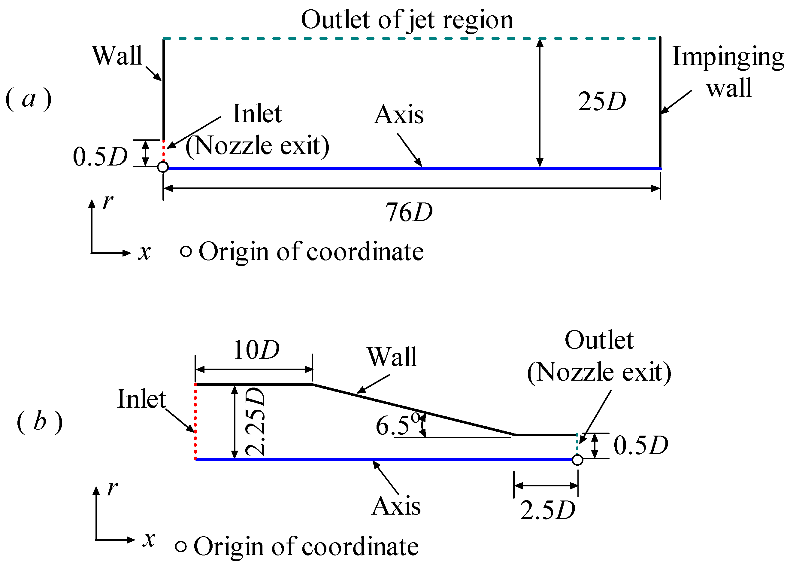
The problem of a high-pressure water jet which comes from a conical nozzle and flows into the air, then vertically impinges on a flat plate, was simulated firstly. The computational model was constructed based on the experiment conducted by Leach et al. [9], which was used to verify the numerical results. By considering the axisymmetric characteristics both in terms of geometry and physics, the problem was simplified to an axisymmetric model. Numerous studies have demonstrated that the nozzle geometry significantly affects the jet flow [2,9,19]. In this work, as a precursor, the water flow within the nozzle was individually simulated, and the flow quantities at the nozzle exit were extracted and applied to the inlet of the computational model of the jet region. A schematic depiction of the model geometry and relevant boundary conditions is shown in Figure 1. Here, D = 1 mm represents the diameter of the inlet (nozzle exit). L = 76D denotes the distance from the inlet (nozzle exit) to the flat plate. H = 25D indicates the lateral dimension of the jet region.
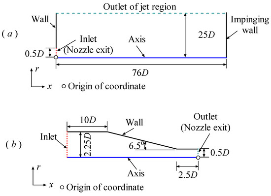
Figure 1.
The schematic depiction of the model geometry of the impinging jet and relevant boundary conditions: (a) jet region; (b) nozzle.
The fluid materials consist of water and air. Their physical properties are listed in Table 1. We have tried using different methods, where either water or air was set as the primary phase separately, and found that our calculations often exhibited instability when air was used as the primary phase. Consequently, in all subsequent simulations, water was selected as the primary phase.

Table 1.
The physical properties of fluids.
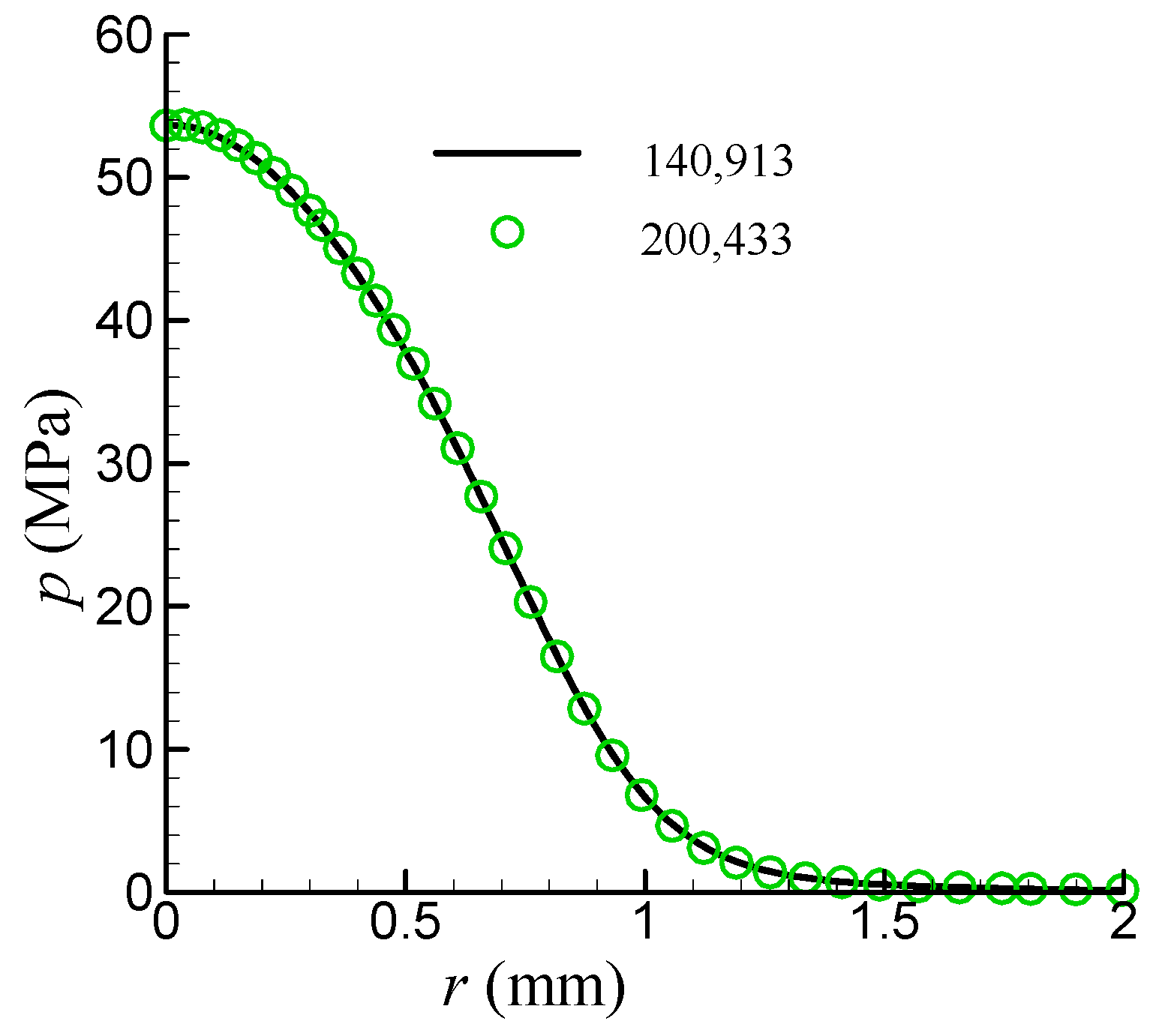
A grid sensitivity analysis was conducted by developing two distinct computational mesh configurations. The second mesh configuration was based on the first one, and the 50 layers of grids adjacent to the flat plate were refined through reducing the grid size by half. The grid numbers of the two configurations are 140,913 and 200,433, respectively. The predicted impact pressure distribution on the flat plate is presented in Figure 2. As can be seen, the difference between the results for the two mesh configurations is indistinguishable, indicating that the simulation results are no longer dependent on the number of grids. Consequently, the first mesh configuration was adopted throughout subsequent simulations to optimize computational efficiency.
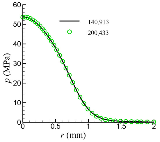
Figure 2.
Comparison of the effects of grid numbers on the impact pressure distribution.
The influences of various factors on the simulation results were investigated. For the convenience of comparative analysis and explanation, a special case was selected as a reference. The results of the reference case show good agreement with the experimental results of Leach et al. [9]. The relevant information for the reference case is listed in Table 2. In the subsequent analysis, unless otherwise specified, when analyzing the influence of a single factor, the other factors remain completely consistent with the reference case.
Table 2.
The information for the reference case.
3.1.2. Effect of Turbulence Treatment Methodologies
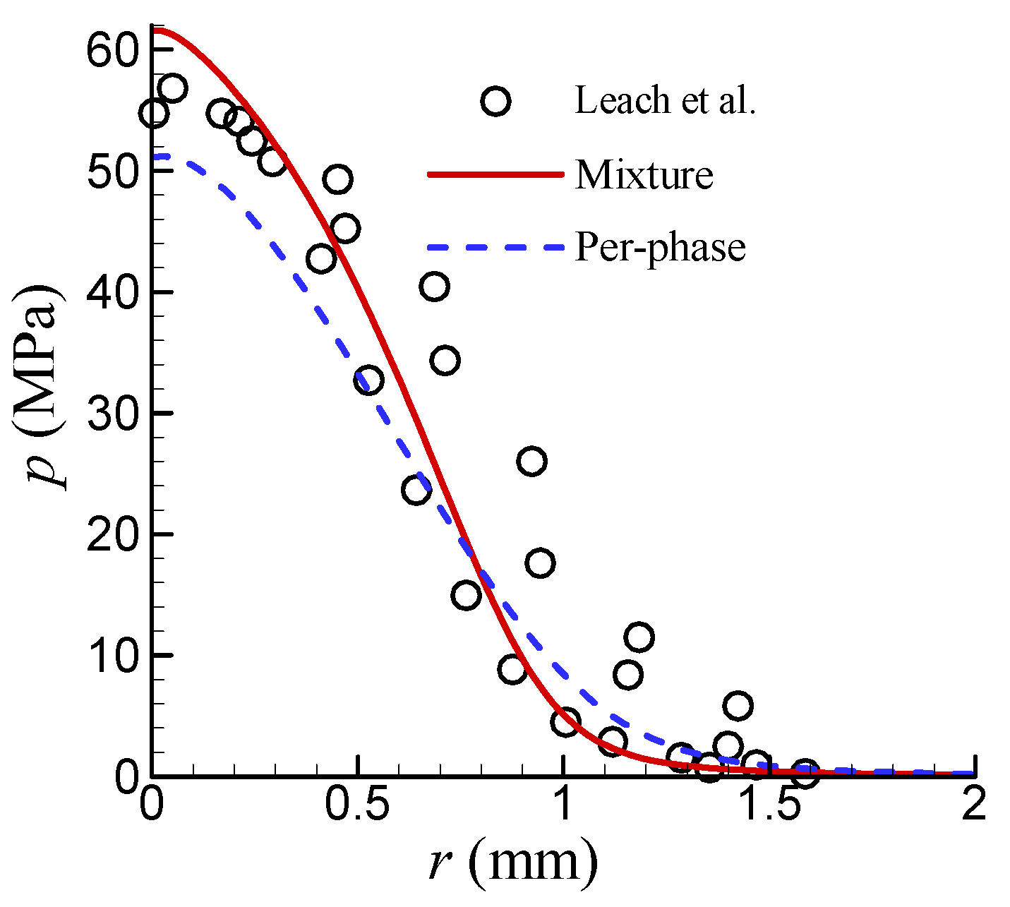
Two turbulence treatment methodologies, namely the mixture turbulence model methodology and the per-phase turbulence model methodology, were investigated. It should be noted that the SST k-ω turbulence model was adopted here because it can be used directly without additional processing in the CFD solver. The distributions of pressure on the flat plate simulated by different methodologies are shown in Figure 3.
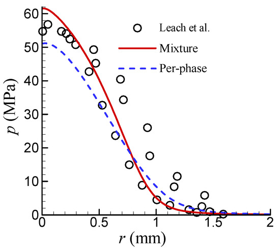
Figure 3.
Comparison of the effects of turbulence treatment methodologies [9].
It is clearly observed that, in the region near the stagnation point, the mixture turbulence model methodology overpredicts the pressure, whereas the per-phase turbulence model methodology underpredicts it. Overall, the result of the mixture turbulence model methodology is slightly superior. Additionally, considering the simplicity and ease of use of the method itself, the mixture turbulence model methodology was chosen in this work.
3.1.3. Effect of Turbulence Models
In the flow of a high-pressure water jet in air, turbulence plays a crucial role. Accurately calculating turbulence will determine the success or failure of the simulation. It is well known that every turbulence model has its own advantages and applicable ranges. Finding and examining turbulence models with good simulation results for high-pressure water impinging jet flows is of great significance in engineering.
Three turbulence models were considered: the SST k-ω-φ-α model, the SST k-ω model, and the realizable k-ε model. In the computations, except for the turbulence models, all other settings were identical to those of the reference case.
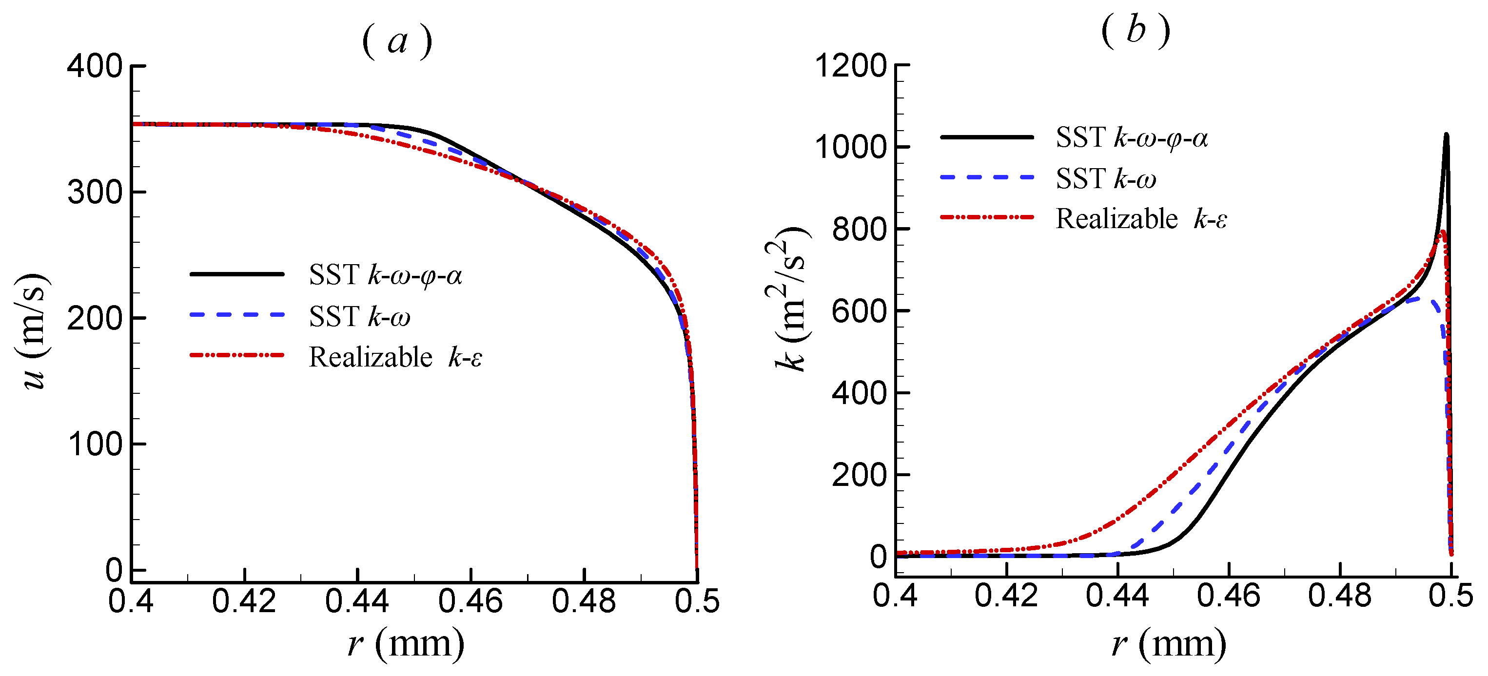
Figure 4 shows the velocity and turbulent kinetic energy profiles at the nozzle exit predicted by different turbulence models. In most areas near the axis (r < 0.4 mm), the results obtained by the three turbulence models are very close. There are some differences in the area near the nozzle wall. Overall, the differences among the velocities obtained by the three turbulence models are not too significant, but the differences in turbulence kinetic energy are quite noticeable. The SST k-ω-φ-α model predicted the largest peak value of the turbulence kinetic energy, while the SST k-ω model predicted the lowest.
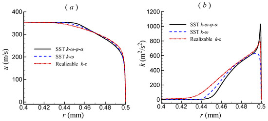
Figure 4.
Velocity and turbulent kinetic energy at nozzle exit predicted by different turbulence models: (a) velocity; (b) turbulent kinetic energy.
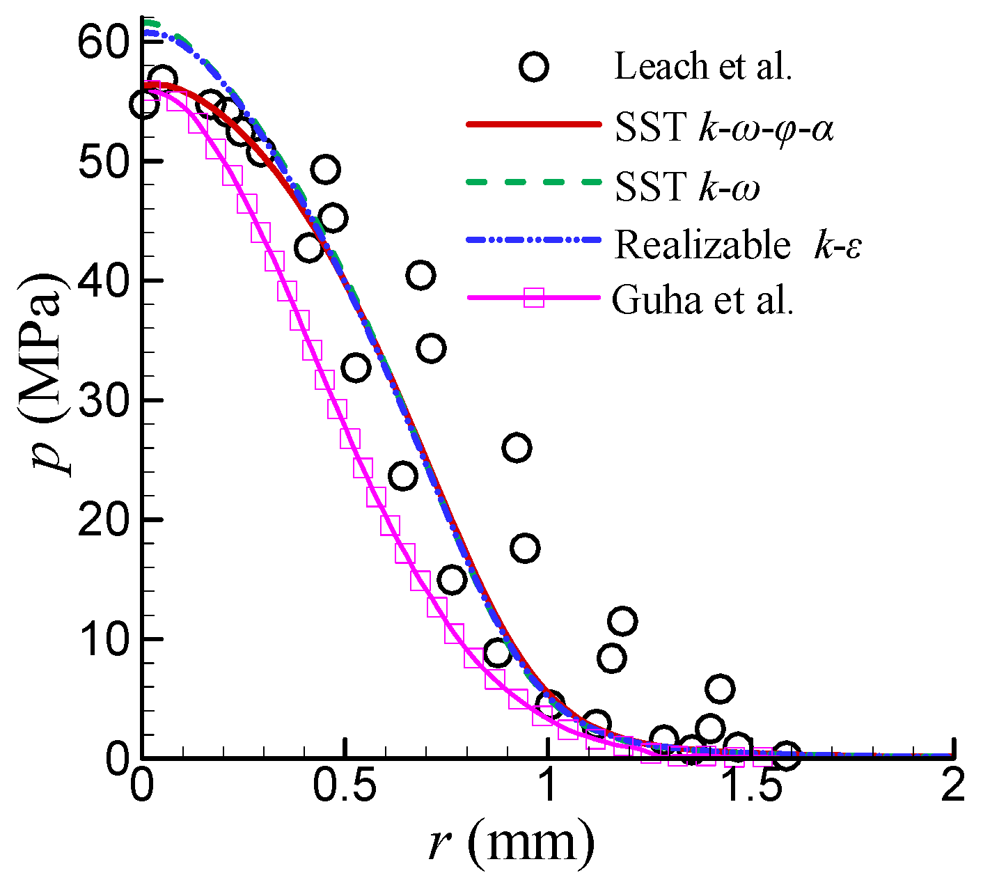
The distributions of pressure on the flat plate simulated by different turbulence models are shown in Figure 5. It is observed that the SST k-ω-φ-α model yields good stagnation pressure compared with the experiments of Leach et al. [9]. The difference between the SST k-ω model and the realizable k-ε model is slight. They overpredicted the pressure near the stagnation point by about 10%. In areas with r > 0.5 mm, the results from the three turbulence models are almost indistinguishable. As a comparison, the pressure distribution on the flat plate from the numerical simulation of Guha et al. [12] is also depicted. Obviously, it was underpredicted throughout.
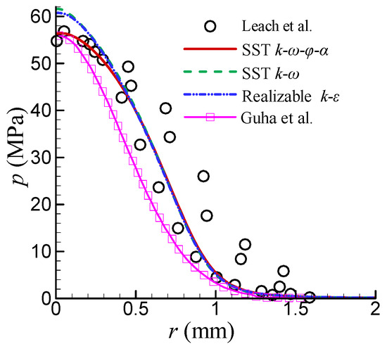
Figure 5.
Comparison of the effects of turbulence models on the pressure distribution [9,12].
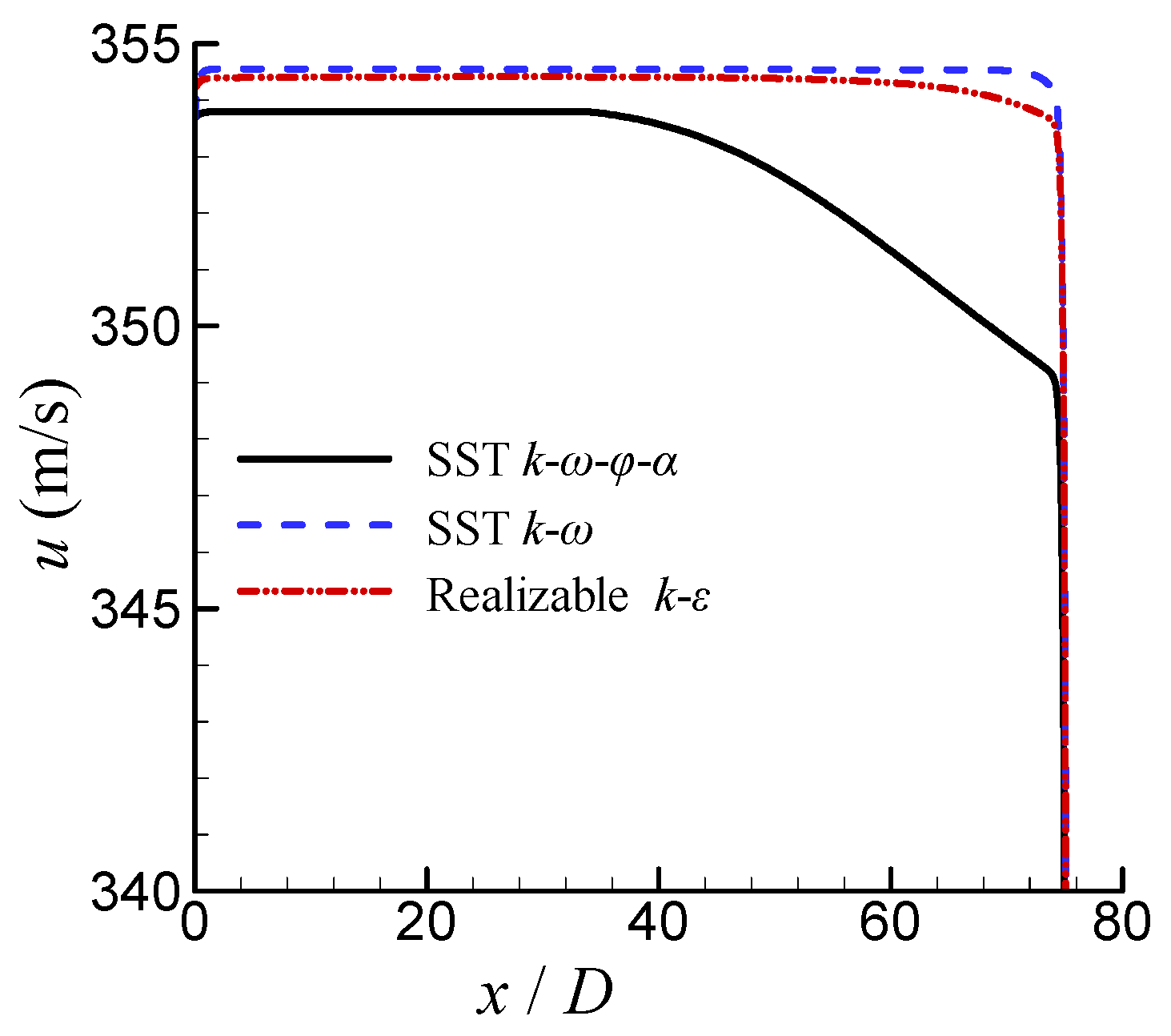
Figure 6 shows the velocity profiles along the axis simulated by different turbulence models. It is clear that the velocity decreases quickly to zero in the vicinity of the flat plate. The major difference is that the jet’s potential core regions (in which the velocity remains constant) obtained by the SST k-ω model and the realizable k-ε model are longer than those obtained by the SST k-ω-φ-α model. The velocity on the axis predicted by the SST k-ω-φ-α model decreases from x ≈ 30D. According to Bernoulli’s equation, the pressure at the stagnation point is , where is the velocity on the axis before impacting the flat plate. The obtained by the SST k-ω-φ-α model is relatively small, so the impact pressure near the stagnation point is also small.
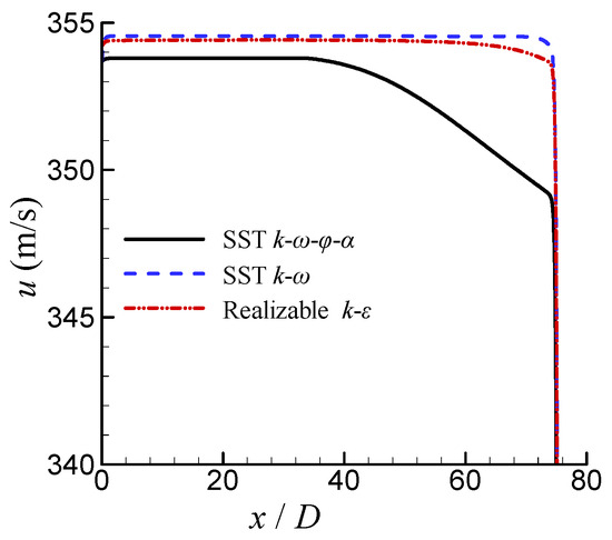
Figure 6.
Comparison of the effects of turbulence models on the velocity along the axis.
In most applications of high-pressure water jets, the pressure distribution near the stagnation point plays a key role; therefore, the SST k-ω-φ-α model is worth recommending.
3.1.4. Effect of Bubble Diameter of the Secondary Phase
When a high-pressure water jet enters the air, under the strong action of shear force, the continuous water stream will break into small water droplets near the interface between water and air. These small water droplets further break down to form water mist [6]. The interaction between small water droplets and air is an important factor in the exchange of momentum between the two phases. The diameter of water droplets has a significant impact on the interfacial force and drag force. In this work, air was selected as the secondary phase, meaning we assumed the presence of air bubbles rather than water droplets near the interface between water and air. From a numerical simulation perspective, this approach is acceptable because the interaction between the two phases is ultimately introduced into the momentum equation in the same way, i.e., as an interfacial force and a drag force. Due to the lack of detailed information on the size of air bubbles, we roughly assumed that the size of air bubbles is uniformly distributed in the flow field.
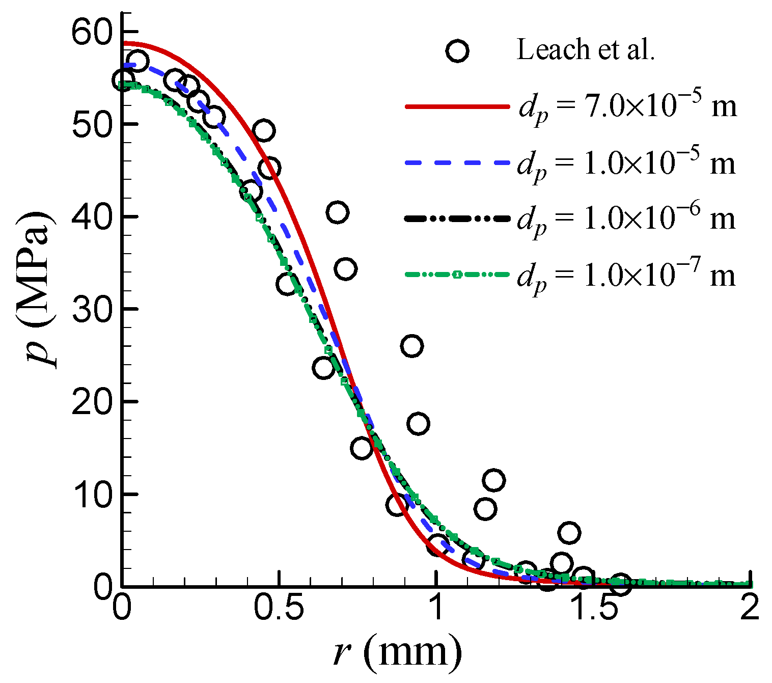
The influence of different diameters of air bubbles was investigated, and the results are shown in Figure 7. As observed, the pressure near the stagnation point becomes higher when the diameter of the air bubbles becomes larger. When the diameter of the bubbles is below a certain size (such as 10−6 m), the pressure almost does not change with the size of the bubble. The reason for this may be that when the diameter of the bubbles is below a threshold, the drag force is so small that it makes almost no contribution to the transfer of momentum. A diameter of 10−5 m yields good results compared to the experiment. It should be pointed out that the largest diameter of bubbles simulated in the present work is 7 × 10⁻⁵ m because the computation becomes unstable when the bubble diameter is larger.

Figure 7.
Comparison of the effect of the bubble diameter of the secondary phase on the pressure distribution [9].
3.1.5. Effect of Surface Tension
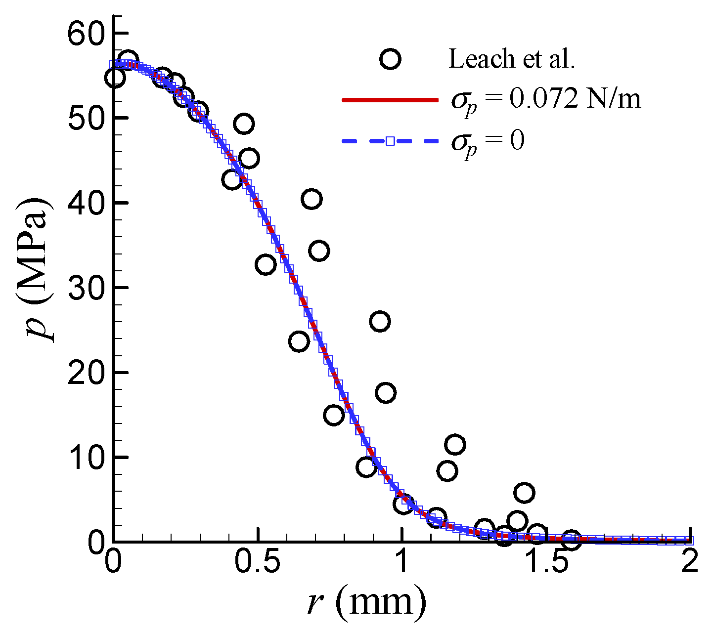
In many problems involving a liquid–gas interface, surface tension may have a significant impact on the flow. However, in the problem of a high-pressure water jet in air, due to the large velocity, the Weber number, We = ρLU2/σ, is very large. As an example, if we set then . Such a large means the surface tension force is very small relative to the inertial force; thus, the effect of surface tension may be neglected. To verify this assertion, two cases were considered. The surface tension coefficient σ = 0.072 N/m in the first case, while σ = 0 in the second case.
Figure 8 quantitatively compares predicted impact pressure profiles across varied surface tension coefficients. The computational data demonstrate that the surface tension has negligible influence on jet impingement dynamics within the studied parameter space.
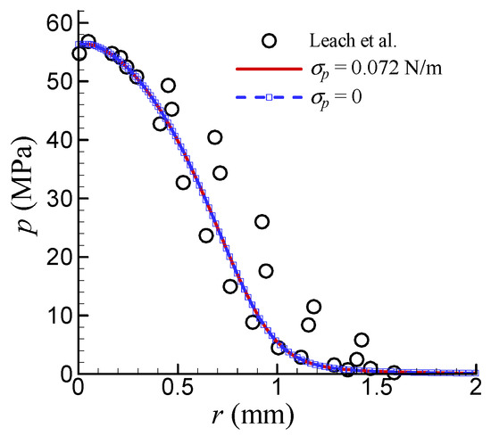
Figure 8.
Comparison of the effect of surface tension on the pressure distribution [9].
3.2. Free Jet
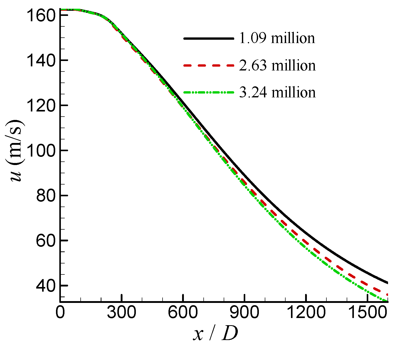
The problem of a free high-pressure water jet was also simulated. The jet issues from a conical nozzle, then flows into the air and sprays over long distances. The computational model was constructed based on the experiments conducted by Rajaratnam et al. [7]. Considering the axisymmetric characteristics both in terms of geometry and physics, it was simplified to an axisymmetric model. A schematic depiction of the model geometry and relevant boundary conditions is shown in Figure 9a. The enlarged view of the nozzle is shown in Figure 9b. Here, the diameter of the nozzle exit D = 2 mm, the length of the main computational domain along the jet stream-wise is 1600D, and the lateral size is 50D. The mean velocity at the nozzle exit is 159 m/s. Other related computational settings are consistent with the reference case. To verify the independence of the simulation results from the grid, three grid configurations were designed through refining cells in the jet region and near the wall boundaries. Based on the different grid configurations, the velocities along the axis computed by the SST k-ω-φ-α model are shown in Figure 10. It can be seen that there is a small difference among the results. In the end, the grid configuration with a grid number of 2.63 million was chosen.
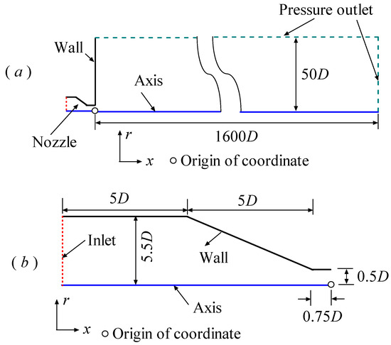
Figure 9.
The schematic depiction of the model geometry of the free jet and the relevant boundary conditions. (a) the whole computational model; (b) enlarged view of the nozzle.

Figure 10.
The velocities along the axis based on the different computational grids.
Simulations using three turbulence models, namely the SST k-ω-φ-α model, the SST k-ω model, and the realizable k-ε model, were performed. Figure 11 compares the simulated velocity (normalized by the mean velocity at the nozzle exit, Unozzle = 159 m/s) from different turbulence models along the axis. Apparently, the velocities predicted by all three turbulence models agree well with the experimental data obtained by Rajaratnam et al. [7] in the region of x < 200D. Moreover, the velocities maintain their value at the nozzle exit, and there is not much difference in the results of the three turbulence models in this region.
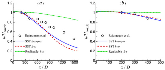
Figure 11.
Comparison of velocity along the axis. (a) x from 0 to 1600D; (b) x from 0 to 500D [7].
When x > 200D, the simulated velocities begin to branch. For the SST k-ω-φ-α model and the SST k-ω model, the results in the region of 200D < x < 400D are still in good agreement with the experimental results. When x > 400D, compared to experiments, the velocities decay more rapidly with increasing distance. Relatively, the velocity decay obtained by the SST k-ω-φ-α model is slower; thus, its results are closer to those of the experiments. However, the simulated results from the realizable k-ε model are completely opposite to those from the SST k-ω-φ-α model and the SST k-ω model, with much slower velocity decay than the experimental results. In the simulation of high-pressure water impinging jets with a short stand-off distance, the difference between the SST k-ω model and the realizable k-ε model is small (see Section 3.1.3). However, in free high-pressure water jets with long ranges, there is a significant difference between the SST k-ω model and the realizable k-ε model. This phenomenon indicates that the realizable k-ε model has a smaller expanding rate than the SST k-ω model.
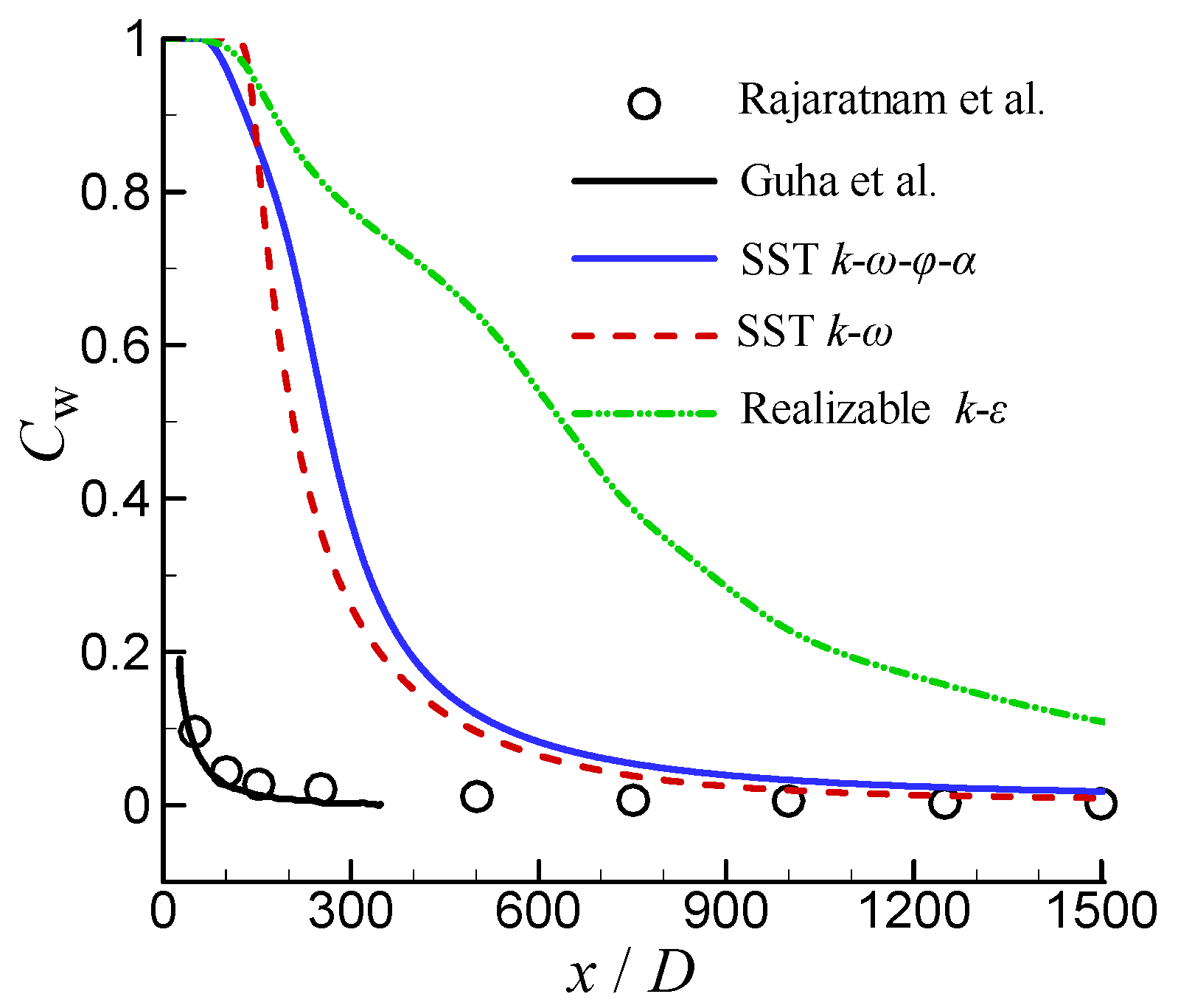
Figure 12 shows the simulated volume fraction of water (Cw) along the axis by different turbulence models. In the experiments of Rajaratnam et al. [8], the volume fraction of water decreased rapidly after the jet left the nozzle, indicating that a large amount of air quickly entered the core area of the jet. The SST k-ω-φ-α model and the SST k-ω model similarly obtained a rapidly decreasing volume fraction of water. The difference is that the length of the jet potential core obtained by these two turbulence models is much larger than the experimental results. Figure 12 also includes the numerical results of Guha et al. [10,12]. They obtained a volume fraction of water consistent with the experiments by introducing additional source terms into the momentum equation. However, as shown in Figure 5, this method reduces the simulation accuracy of the impact pressure distribution for an impinging jet with a short stand-off distance. The realizable k-ε model obtained a different behavior; i.e., the simulated water volume fraction decreased much more slowly with increasing distance.

Figure 12.
Comparison of volume fraction of water along the axis [8,10,12].
Overall, in high-pressure water jets with short ranges, the simulation results are in good agreement with the experiments. But as the distance increases, the deviation becomes larger. A reason for this may be that the method utilized in this work does not consider the processes of the formation, deformation, and fragmentation of the water droplets in high-pressure water jets. This process is undoubtedly important for long-distance water jets. Further improvements can be made in future work.
4. Conclusions
Based on the Eulerian multiphase flow model, high-pressure water impinging jets in air and free high-pressure water jets in air were numerically simulated. The methods of turbulence treatment, the effects of different turbulence models, the influence of the bubble diameter of the secondary phase, and the effects of surface tension were thoroughly investigated. The results led to the following conclusions:
- (1)
- The mixture turbulence model methodology not only has simple governing equations and is easy to use, but also can yield good results, making it suitable for simulating high-pressure water jets.
- (2)
- For high-pressure water impinging jets in air, comparatively, the SST k-ω-φ-α model yielded the best results. Both the realizable k-ε model and the SST k-ω model slightly overpredicted the pressure near the stagnation point.
- (3)
- The bubble diameter of the secondary phase has an influence on the impact pressure. The impact pressure decreases as the bubble diameter decreases. However, the bubble diameter has less effect on the impact pressure after it decreases below a threshold.
- (4)
- Surface tension has a negligible effect on the impact pressure of high-pressure water impinging jets with a small stand-off distance.
- (5)
- For free high-pressure water jets with long ranges, the difference between the SST k-ω-φ-α model and the SST k-ω model is not large. The results of the realizable k-ε model are quite different from those of the other two models, and they are not consistent with the trend of the experiments. Relatively, the results of the SST k-ω-φ-α model are better.
The main focus of this work is to investigate several key factors which affect the numerical simulation of high-pressure water jets in air. The obtained results can help to establish a dual-pronged framework that synergistically integrates computational mechanics with predictive modeling methodologies. From a theoretical perspective, the proposed model enables precise prediction of multiphase flow dynamics and material interaction mechanisms inherent to high-pressure water jet cleaning and cutting processes through combinging with rigorous solid mechanics computations. From a technological perspective, the rapid advancement of artificial intelligence (AI) and machine learning (ML) algorithms holds significant potential for revolutionizing operational parameter optimization in water jet applications. Specifically, this research can help to generate comprehensive datasets—encompassing fluid velocity fields, pressure distribution patterns, and volume of fraction characteristics—so it serves as a critical foundation for training robust ML architectures. This dual contribution can not only advance our fundamental understanding of fluid–structure interactions but can also support autonomous, data-driven decision-making systems in next-generation industrial water jet technologies.
Author Contributions
Conceptualization, X.Y. and L.Y.; methodology, X.Y.; software, X.Y.; validation, L.Y.; writing—original draft preparation, X.Y.; writing—review and editing, L.Y.; project administration, L.Y.; funding acquisition, L.Y. All authors have read and agreed to the published version of the manuscript.
Funding
This research was funded by the National Key R&D Program of China (Grant No. 2022YFC3800904) and the Natural Science Foundation of Shenzhen, China (Grant No. 20220809155933002).
Data Availability Statement
The original contributions presented in this study are included in the article. Further inquiries can be directed to the corresponding author.
Conflicts of Interest
The authors declare no conflicts of interest.
References
- Liu, F.; Wang, Y.; Huang, X. Cutting efficiency of extremely hard granite by high-pressure water jet and prediction model of cutting depth based on energy method. Bull. Eng. Geol. Environ. 2024, 83, 95. [Google Scholar] [CrossRef]
- Chen, L.; Cheng, M.; Cai, Y.; Guo, L.; Gao, D. Design and optimization of high-pressure water jet for coal breaking and punching nozzle considering structural parameter interaction. Machines 2022, 10, 60. [Google Scholar] [CrossRef]
- Liu, L.; Xu, X.; Meng, Z.; Lv, H.; Liu, F. Exploration on application of high pressure water jet cleaning technology. MATEC Web Conf. 2021, 353, 01006. [Google Scholar] [CrossRef]
- Szada–Borzyszkowska, M.; Kacalak, W.; Banaszek, K.; Pude, F.; Perec, A.; Wegener, K. Assessment of the effectiveness of high–pressure water jet machining generated using self-excited pulsating heads. Int. J. Adv. Manuf. Technol. 2024, 133, 5029–5051. [Google Scholar] [CrossRef]
- Leu, M.C.; Meng, P.; Geskin, E.S.; Tismeneskiy, L. Mathematical modeling and experimental verification of stationary waterjet cleaning process. J. Manuf. Sci. Eng. 1998, 120, 571–579. [Google Scholar] [CrossRef]
- Jiang, M.; Wang, F.; Yuan, M.; Liu, Y.; Xiong, J.; Niu, Y.; Long, Z. Analysis of the whole main structure morphological evolution and velocity distribution characteristics of a high-pressure water jet by an imaging experiment. Measurement 2023, 214, 112817. [Google Scholar] [CrossRef]
- Rajaratnam, N.; Rizvi, S.A.H.; Steffler, P.M.; Smy, P.R. An experimental study of very high velocity circular water jets in air. J. Hydraul. Res. 1994, 32, 461–470. [Google Scholar] [CrossRef]
- Rajaratnam, N.; Albers, C. Water distribution in very high velocity water jets in air. J. Hydraul. Eng. 1998, 124, 647–650. [Google Scholar] [CrossRef]
- Leach, S.J.; Walker, G.L.; Smith, A.V.; Farmer, I.W.; Taylor, G. Some aspects of rock cutting by high speed water jets [and Discussion]. Philos. Trans. R. Soc. London. Ser. A Math. Phys. Sci. 1966, 260, 295–310. [Google Scholar]
- Guha, A.; Barron, R.M.; Balachandar, R. An experimental and numerical study of water jet cleaning process. J. Mater. Process Tech. 2011, 211, 610–618. [Google Scholar] [CrossRef]
- Liu, H.; Wang, J.; Kelson, N.; Brown, R.J. A study of abrasive waterjet characteristics by CFD simulation. J. Mater. Process Tech. 2004, 153–154, 488–493. [Google Scholar] [CrossRef]
- Guha, A.; Barron, R.M.; Balachandar, R. Numerical simulation of high-speed turbulent water jets in air. J. Hydraul. Res. 2010, 48, 119–124. [Google Scholar] [CrossRef]
- Liu, H.-x.; Shao, Q.-m.; Kang, C.; Gong, C. Impingement capability of high–pressure submerged water jet: Numerical prediction and experimental verification. J. Cent. South. Univ. 2015, 22, 3712–3721. [Google Scholar] [CrossRef]
- Behnia, M.; Parneix, S.; Shabany, Y.; Durbin, P.A. Numerical study of turbulent heat transfer in confined and unconfined impinging jets. Int. J. Heat Fluid Flow 1999, 20, 1–9. [Google Scholar] [CrossRef]
- Bovo, M.; Davidson, L. On the Numerical Modeling of Impinging Jets Heat Transfer—A Practical Approach. Numer. Heat. Tr. A-Appl. 2013, 64, 290–316. [Google Scholar] [CrossRef]
- Khalaji, E.; Nazari, M.R.; Seifi, Z. 2D numerical simulation of impinging jet to the flat surface by turbulence model. Heat. Mass. Transfer 2016, 52, 127–140. [Google Scholar] [CrossRef]
- Yang, X.L.; Liu, Y.; Yang, L. A shear stress transport incorporated elliptic blending turbulence model applied to near-wall, separated and impinging jet flows and heat transfer. Comput. Math. Appl. 2020, 79, 3257–3271. [Google Scholar] [CrossRef]
- Menter, F.; Ferreira, J.C.; Esch, T.; Konno, B. The SST turbulence model with improved wall treatment for heat transfer predictions in gas turbines. In Proceedings of the International Gas Turbine Congress 2003, Tokyo, Japan, 2–7 November 2003. [Google Scholar]
- Urazmetov, O.; Cadet, M.; Teutsch, R.; Antonyuk, S. Investigation of the flow phenomena in high-pressure water jet nozzles. Chem. Eng. Res. Des. 2021, 165, 320–332. [Google Scholar] [CrossRef]


Disclaimer/Publisher’s Note: The statements, opinions and data contained in all publications are solely those of the individual author(s) and contributor(s) and not of MDPI and/or the editor(s). MDPI and/or the editor(s) disclaim responsibility for any injury to people or property resulting from any ideas, methods, instructions or products referred to in the content. |
© 2025 by the authors. Licensee MDPI, Basel, Switzerland. This article is an open access article distributed under the terms and conditions of the Creative Commons Attribution (CC BY) license (https://creativecommons.org/licenses/by/4.0/).