Enhanced Estimation of the Unit Lindley Distribution Parameter via Ranked Set Sampling with Real-Data Application

Abstract

This paper investigates various estimation methods for the parameters of the unit Lindley distribution (U-LD) under both ranked set sampling (RSS) and simple random sampling (SRS) designs. The distribution parameters are estimated using the maximum likelihood estimation, ordinary least squares, weighted least squares, maximum product of spacings, minimum spacing absolute distance, minimum spacing absolute log-distance, minimum spacing square distance, minimum spacing square log-distance, linear-exponential, Anderson–Darling (AD), right-tail AD, left-tail AD, left-tail second-order, Cramér–von Mises, and Kolmogorov–Smirnov. A comprehensive simulation study is conducted to assess the performance of these estimators, ensuring an equal number of measuring units across both designs. Additionally, two real datasets of items failure time and COVID-19 are analyzed to illustrate the practical applicability of the proposed estimation methods. The findings reveal that RSS-based estimators consistently outperform their SRS counterparts in terms of mean squared error, bias, and efficiency across all estimation techniques considered. These results highlight the advantages of using RSS in parameter estimation for the U-LD distribution, making it a preferable choice for improved statistical inference.

1. Introduction

The study of probability distributions continues to be a vibrant area within statistical modeling. Recent years have seen growing interest in developing specialized distributions that effectively model data confined to the interval [0, 1]. These “unit distributions” are particularly valuable for analyzing probabilities, proportions, and percentages—quantities that frequently arise in medical research, actuarial science, and financial analysis. The literature has witnessed a proliferation of novel unit distributions. Notable examples include the unit-inverse Gaussian distribution in [1], the unit-Gompertz distribution in [2], the unit log-log distribution in [3], the unit-Weibull distribution propsed in [4], the unit Burr-XII distribution offered in [5], the unit-Chen distribution in [6], the unit generalized half normal distribution suggested in [7], the unit-Muth distribution offered in [8], and the unit Birnbaum–Saunders distribution in [9]. Ref. [10] suggests the unit two-parameter Mirra distribution, and Ref. [11] proposes the unit power BurrX distribution.

Thus, Ref. [12] introduces the U-LD through a transformation of the classic Lindley distribution. The U-LD has proven to be a powerful statistical tool for analyzing data within the $[0,1]$ interval, distinguished by its mathematical properties and practical utility. As a member of the exponential family of distributions, it offers closed-form expressions for its moments, significantly simplifying statistical inference and analysis. The distribution’s theoretical framework has been enriched through various contributions, including the development of complete and incomplete moment expressions in [13], an exponential variant that provides enhanced modeling flexibility [14], and applications in reliability theory through stress-strength modeling where $P(Y<X)$ is of interest [15]. These mathematical properties, combined with successful implementations in fields such as public health research, demonstrate the distribution’s versatility in addressing real-world analytical challenges while maintaining computational tractability. Ref. [16] advances the field by investigating parameter estimation in unit Lindley mixed effect models, specifically addressing the challenges posed by clustered and longitudinal proportional data. 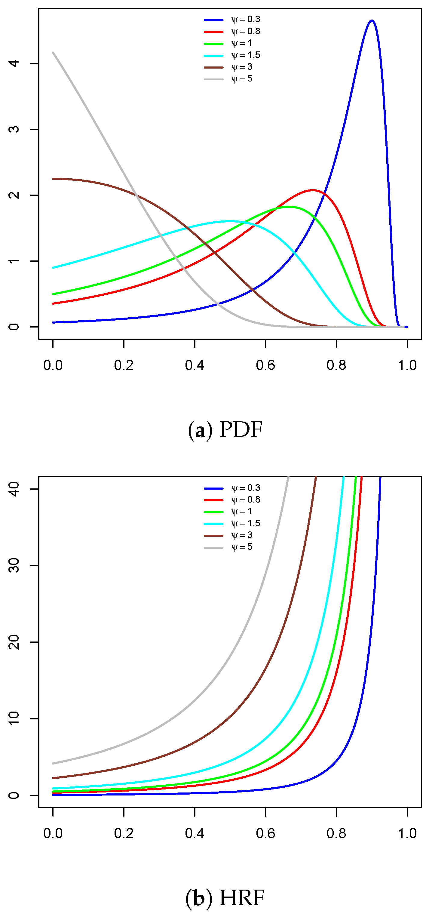Bayesian inference of the three-component unit Lindley right censored mixture is presented in [17]. The probability density function (PDF) of the U-LD [12] is defined by

$$g\left(w\right)={\displaystyle \frac{{\psi }^2}{\left(\psi +1\right){\left(w-1\right)}^3}}{\mathrm{e}}^{-{\displaystyle \frac{\psi w}{1-w}}};,0<w<1,\psi >0.$$

(1)

The cumulative distribution function (CDF) and hazard rate function (HRF) of the U-LD are given, respectively, by

$$G\left(w\right)=1-\left(1-{\displaystyle \frac{\psi w}{\left(\psi +1\right)\left(w-1\right)}}\right){\mathrm{e}}^{-{\displaystyle \frac{\psi w}{1-w}}}0<w<1,\psi >0,$$

(2)

and

$$h\left(w\right)={\displaystyle \frac{{\psi }^2}{(\psi -w+1){(w-1)}^2}},0<w<1.$$

Figure 1 shows both the PDF and HRF for the U-LD distribution. The density function exhibits a unimodal shape, increasing–decreasing, and decreasing. Additionally, the hazard rate function demonstrates a monotonically increasing pattern.

The RSS emerged as an innovative approach to population mean estimation, improving upon traditional SRS methods. First introduced in [18], RSS shines in its ability to capture more representative samples of target populations, delivering superior accuracy while saving both resources and time. The technique’s theoretical underpinnings were developed later in [19], where mathematical proof was provided that RSS mean estimators maintain unbiasedness while achieving better precision compared to SRS estimates under perfect ranking conditions. Ref. [20] further strengthens these findings by showing that RSS maintains its advantages even when ranking procedures are not perfect. The work demonstrates the method’s robustness and practical utility across various real-world scenarios where perfect ranking might not be feasible. Readers may consult references [21,22].

Over the past forty years, RSS has attracted considerable interest in statistical research, particularly in parameter estimation for various parametric families. Numerous studies have applied RSS to estimate unknown parameters. For example, Ref. [23] estimates logistic model parameters using both SRS and RSS, demonstrating the efficiency gains of RSS in parameter estimation.

Ref. [24] applies RSS to estimate the parameters of the Gumbel distribution, highlighting its advantages over traditional methods. Ref. [25] investigates the estimation of $P(X<Y)$ for the Weibull distribution using RSS, providing insights into improved estimation accuracy. Ref. [26] employs both Bayesian and maximum likelihood estimation approaches to determine the parameters of the Kumaraswamy distribution under RSS. Ref. [27] suggests best linear unbiased and invariant estimation in location-scale families based on double RSS, while Ref. [28] further explores Bayesian inference for the same distribution. Ref. [29] proposed generalizes robust-regression-type estimators under different RSS. Ref. [30] focuses on efficient parameter estimation for the generalized quasi-Lindley distribution under RSS, demonstrating its practical applications. Ref. [31] examines RSS-based estimation for the two-parameter Birnbaum–Saunders distribution, contributing to the broader literature on RSS efficiency. Additionally, Ref. [32] provides an efficient stress–strength reliability estimate for the unit Gompertz distribution using RSS. Ref. [33] considers the problem of estimating the parameter of Farlie–Gumbel–Morgenstern bivariate Bilal distribution by RSS. Ref. [34] investigates the moving extreme RSS and MiniMax RSS for estimating the distribution function, and Ref. [35] investigates parameter estimation for the exponential Pareto distribution under ranked and double-ranked set sampling designs, showcasing the effectiveness of these sampling strategies in reliability analysis.

Interested in the widespread applications of the RSS method across various fields, this study focuses on estimating the parameters of the U-LD. To achieve this, we employ several classical estimation approaches based on both RSS and SRS. The estimation techniques considered include maximum likelihood estimation (MLE), ordinary least squares (OLS), weighted least squares (WLS), maximum product of spacings (MPS), minimum spacing absolute distance (MSAD), minimum spacing absolute log-distance (MSALD), minimum spacing square distance (MSSD), minimum spacing square log-distance (MSSLD), linear-exponential (Linex), Anderson–Darling, right-tail AD (RAD), left-tail AD (LAD), left-tail second-order (LTS), Cramér–von Mises (CV), and Kolmogorov–Smirnov (KS).

To the best of our knowledge, this is the first study that considers the parameter estimation of the unit Lindley distribution using RSS. The proposed estimators under RSS are systematically compared with their SRS counterparts through simulation studies that assess their precision based on bias, mean squared error (MSE), and mean absolute relative error. Additionally, a real dataset is analyzed to demonstrate the practical effectiveness of the RSS-based estimators.

The structure of this paper is as follows: The RSS is defined in Section 2, Section 3 presents the estimation methods for the U-LD, while Section 4 conducts a simulation study to evaluate and compare the performance of the proposed estimators. Section 5 provides an analysis of a real dataset, and finally Section 6 concludes with key remarks and insights.

2. Description of the RSS Scheme

We assume that the random variable of interest W has a PDF $h\left(w\right)$ and CDF H(w). To illustrate the RSS procedure, we follow these steps:

Step 1: Select m SRS each of size m as

$W_{11}$,	$W_{12}$,	...,	$W_{1m}$
$W_{21}$,	$W_{22}$,	...,	$W_{2m}$
⋮	⋮	⋮	⋮
$W_{m1}$,	$W_{m2}$,	...,	$W_{mm}$

Step 2: Rank the unit within each set based on the variable of interest using visual inspection, expert judgment, or any inexpensive ranking method (without actual measurement) as

$W_{1(1:m)}$,	$W_{1(2:m)}$,	...,	$W_{1(m:m)}$
$W_{2(1:m)}$,	$W_{2(2:m)}$,	...,	$W_{2(m:m)}$
⋮	⋮	⋮	⋮
$W_{m(1:m)}$,	$W_{m(2:m)}$,	...,	$W_{m(m:m)}$

Step 3: Choose the sth ranked unit from the sth set as

$\left[W_{1(1:m)}\right]$,	$W_{1(2:m)}$,	...,	$W_{1(m:m)}$
$W_{2(1:m)}$,	$\left[W_{2(2:m)}\right]$,	...,	$W_{2(m:m)}$
⋮	⋮	⋮	⋮
$W_{m(1:m)}$,	$W_{m(2:m)}$,	...,	$\left[W_{m(m:m)}\right]$

Hence, the RSS units are $W_{1(1:m)}$, $W_{2(2:m)}$,..., $W_{m(m:m)}$. Note that we identify $m^2$ units but only measure m of them. To increase the sample size, we extend Steps (1) through (3) to multiple cycles to construct a RSS sample of size $n=mr$. In this case, the RSS sample observations are denoted as $w_{s(s:m)u},s=1,2,\dots ,m,u=1,2,\dots ,r.$ The process of designing a RSS scheme involves selecting an optimal set size, typically limited to a maximum of five to reduce ranking errors.

For a fixed u, the elements $W_{s(s:m)u}$ are independent and follow the same distribution as the sth order statistic from a sample of size m. The PDF of $W_{s(s:m)u}$, assuming perfect ranking as described by Arnold et al. [36], is given by

$$h\left(w_{s(s:m)u}\right)={\displaystyle \frac{1}{B(s,m-s+1)}}{\left[H\left(w_{s(s:m)u}\right)\right]}^{s-1}{\left[1-H\left(w_{s(s:m)u}\right)\right]}^{m-s}h\left(w_{s(s:m)u}\right),w_{s(s:m)u}\in R,$$

(3)

where $h\left(w_{s(s:m)u}\right)$ and $H\left(w_{s(s:m)u}\right)$ denote the PDF and CDF of W, respectively.

3. Methods of Estimation

This section aims to provide a detailed description of the RSS and derive the estimator of UL-D using different methods of estimation under RSS.

3.1. Maximum Likelihood Estimation

We let $w_{s(s:m)u},s=1,2,\dots ,m,u=1,2,\dots ,r$ be the RSS of size $n=mr$ where m is the set size and r is number of cycles, gathered form the U-LD. The likelihood function of the U-LD is obtained by inserting Equations (1) and (2) in Equation (3) as below:

$$L\left(\alpha \right)\propto \prod _{s=1}^m\prod _{u=1}^r{\left[\Omega (w_{s(s:m)u},\psi )\right]}^{s-1}{\left[1-\Omega (w_{s(s:m)u},\psi )\right]}^{m-s}{\displaystyle \frac{{\psi }^2{\mathrm{e}}^{\frac{\psi w_{s(s:m)u}}{w_{s(s:m)u}-1}}}{\left(\psi +1\right){\left(1-w_{s(s:m)u}\right)}^3}},$$

(4)

where $\Omega (w_{s(s:m)u},\psi )=\left(1-{\displaystyle \frac{\psi w_{s(s:m)u}}{\left(\psi +1\right)\left(w_{s(s:m)u}-1\right)}}\right){\mathrm{e}}^{-{\displaystyle \frac{\psi w_{s(s:m)u}}{1-w_{s(s:m)u}}}}.$

The logarithmic of Equation (4), indicated by $l\left(\psi \right),$ is expressed by

$$\begin{array}{c}l\left(\psi \right)\propto 2nlog\psi -nlog(\psi +1)-\psi {\displaystyle \sum _{s=1}^m}{\displaystyle \sum _{u=1}^r}{\displaystyle \frac{w_{s(s:m)u}}{1-w_{s(s:m)u}}}\hfill \\ +{\displaystyle \sum _{s=1}^m}{\displaystyle \sum _{u=1}^r}\left\{(s-1)log\left[\Omega (w_{s(s:m)u},\psi )\right]+(m-s)log\left[1-\Omega (w_{s(s:m)u},\psi )\right]-3log\left(1-w_{s(s:m)u}\right)\right\}.\hfill \end{array}$$

(5)

We differentiate Equation (5) with respect to $\psi$ and equate it to zero, which results in

$${\displaystyle \frac{\partial l\left(\psi \right)}{\partial \psi }}={\displaystyle \frac{2n}{\psi }}-{\displaystyle \frac{n}{\psi +1}}-\sum _{s=1}^m\sum _{u=1}^r{\displaystyle \frac{w_{s(s:m)u}}{1-w_{s(s:m)u}}}+\sum _{s=1}^m\sum _{u=1}^r\left[{\displaystyle \frac{(s-1){{\Omega }^{\prime }}_{\psi }(w_{s(s:m)u},\psi )}{\Omega (w_{s(s:m)u},\psi )}}-{\displaystyle \frac{(q-s){{\Omega }^{\prime }}_{\psi }(w_{s(s:m)u},\psi )}{1-\Omega (w_{s(s:m)u},\psi )}}\right]=0,$$

(6)

where ${\Omega }_{\psi }^{\prime }(w_{s(s:m)u},\psi )={\displaystyle \frac{\partial {\Omega }_{\psi }(w_{s(s:m)u},\psi )}{\partial \psi }}={\displaystyle \frac{{\psi }^2{\mathrm{e}}^{-\frac{\psi w_{s(s:m)u}}{1-w_{s(s:m)u}}}}{\left(\psi +1\right){\left(w_{s(s:m)u}-1\right)}^3}}.$ The MLE $\stackrel{⌢}{\pi }$ of $\psi$ is the solution of non-linear Equation (6). It seems that Equation (6) has no analytical solution; therefore, one can use a numerical method for obtaining $\stackrel{⌢}{\psi }$.

3.2. Least Square Estimators

In this part, the OLS and WLS are derived using the RSS framework. Ref. [37] introduced the OLS and WLS for estimating the parameters of the beta distribution. We consider an ordered sample $W_{(1:n)},W_{(2:n)},\dots ,W_{(n:n)}$ which forms an RSS of size $n=mr$ collected from the U-LD. By minimizing the respective objective functions with respect to $\psi$, the OLSE ${\widehat{\psi }}_{OLS}$ and WLSE ${\widehat{\psi }}_{WLS}$ are obtained. The objective functions to be minimized are given by

$$\begin{array}{c}\Lambda \left(\psi \right)={\displaystyle \sum _{s=1}^n}{\left[G\left(w_{(s:n)}\left|\psi \right.\right)-{\displaystyle \frac{s}{n+1}}\right]}^2,\hfill \\ \Phi \left(\psi \right)={\displaystyle \sum _{s=1}^n}{\displaystyle \frac{{(n+1)}^2(n+2)}{s(n-s+1)}}{\left[G\left(w_{(s:n)}\left|\psi \right.\right)-{\displaystyle \frac{s}{n+1}}\right]}^2.\hfill \end{array}$$

The non-linear equations below may be solved to obtain ${\widehat{\psi }}_{OLS}$ and ${\widehat{\psi }}_{WLS}$:

$$\begin{array}{c}{\displaystyle \frac{\partial \Lambda \left(\psi \right)}{\partial \psi }}={\displaystyle \sum _{s=1}^n}\left[G\left(w_{(s:n)}\left|\psi \right.\right)-{\displaystyle \frac{s}{n+1}}\right]\Delta \left(w_{(s:n)}\left|\psi \right.\right)=0,\hfill \\ {\displaystyle \frac{\partial \Phi \left(\psi \right)}{\partial \psi }}={\displaystyle \sum _{s=1}^n}{\displaystyle \frac{{(n+1)}^2(n+2)}{s(n-s+1)}}\left[G\left(w_{(s:n)}\left|\psi \right.\right)-{\displaystyle \frac{s}{n+1}}\right]\Delta \left(w_{(s:n)}\left|\psi \right.\right)=0,\hfill \end{array}$$

where

$$\Delta \left(w_{(s:n)}\left|\psi \right.\right)={\displaystyle \frac{\partial }{\partial \psi }}G\left(w_{(s:n)}\left|\psi \right.\right)={\displaystyle \frac{w_{(s:n)}\psi \left(\psi -w_{(s:n)}+2\right){\mathrm{e}}^{-\frac{w_{(s:n)}\psi }{1-w_{(s:n)}}}}{{\left(w_{(s:n)}-1\right)}^2{\left(\psi +1\right)}^2}}.$$

(7)

3.3. Maximum Product of Spacing Estimator

The MPS method emerged as a powerful alternative to traditional maximum likelihood (ML) estimation through the groundbreaking work in [38,39]. The research revealed that MPS offers distinct advantages in parameter estimation for continuous univariate distributions. Notably, MPS demonstrates broader consistency than ML methods while maintaining equivalent efficiency to MLE.

We consider an ordered sample $W_{(1:n)},W_{(2:n)},\dots ,W_{(n:n)}$ that forms an RSS of size $n=mr$, collected from the U-LD. The corresponding uniform spacings are defined as

$${\Pi }_s\left(\psi \right)=G\left(w_{(s:n)}\left|\psi \right.\right)-G\left(w_{(s-1:n)}\left|\psi \right.\right),i=1,2,...,n+1.$$

where the boundary conditions hold: $G\left(w_{(0:n)}\left|\psi \right.\right)=0,G\left(w_{(n+1:n)}\left|\psi \right.\right)=1,$ ensuring that the sum of spacings satisfies ${\displaystyle \sum _{s=1}^{n+1}}{\Pi }_s\left(\psi \right)=1.$

The MPSE ${\widehat{\psi }}_{MPS}$ of $\psi$ is produced by maximizing the following function with respect to $\psi$:

$${\rm Y}={\displaystyle \frac{1}{n+1}}\sum _{s=1}^{n+1}log\left[{\Pi }_s\left(\psi \right)\right].$$

The MPSE ${\widehat{\psi }}_{MPS}$ is determined by solving the following equation numerically:

$${\displaystyle \frac{\partial {\rm Y}}{\partial \psi }}={\displaystyle \frac{1}{n+1}}\sum _{s=1}^{n+1}{\displaystyle \frac{1}{{\Pi }_s\left(\psi \right)}}\left[\Delta \left(w_{(s:n)}\left|\psi \right.\right)-\Delta \left(w_{(s-1:n)}\left|\psi \right.\right)\right]=0,$$

where $\Delta \left(.\left|\psi \right.\right)$ is given in Equation (7).

3.4. Minimum Spacing Distance Estimators

This section explores diverse parameter estimators for the U-LD distribution using RSS. We let $W_{(1:n)},W_{(2:n)},...,W_{(n:n)}$ be an ordered sample forming RSS of size $n=mr$ collected from the U-LD. Below are five distinct estimation methods, each characterized by its unique objective function and mathematical formulation.

• The MSAD Estimator: This method utilizes the absolute distance between spacings to estimate parameters. Its objective function is defined as

  $${\zeta }_1\left(\psi \right)=\sum _{s=1}^{n+1}\left|{{\rm Y}}_s\left(\psi \right)-{\displaystyle \frac{1}{n+1}}\right|.$$
  The parameter estimation ${\widehat{\psi }}_{MSAD}$ is achieved by solving the corresponding nonlinear equation:

  $${\displaystyle \frac{\partial {\zeta }_1\left(\psi \right)}{\partial \psi }}=\sum _{s=1}^{n+1}{\displaystyle \frac{\left|{{\rm Y}}_s\left(\psi \right)-\frac{1}{n+1}\right|}{{{\rm Y}}_s\left(\psi \right)-\frac{1}{n+1}}}\left[\Delta \left(w_{(s:n)}\left|\psi \right.\right)-\Delta \left(w_{(s-1:n)}\left|\psi \right.\right)\right]=0,$$
• The MSALD Estimator: The MSALD approach incorporates logarithmic transformation to enhance estimation accuracy, particularly for skewed distributions. Its objective function is

  $${\zeta }_2\left(\psi \right)=\sum _{s=1}^{n+1}\left|log\left({{\rm Y}}_s\left(\psi \right)\right)-log\left({\displaystyle \frac{1}{n+1}}\right)\right|.$$
  Equivalently, ${\widehat{\psi }}_{MSALD}$ can be obtained by empirically solving the following nonlinear equation:

  $${\displaystyle \frac{\partial {\zeta }_2\left(\psi \right)}{\partial \psi }}=\sum _{s=1}^{n+1}{\displaystyle \frac{\left|log\left({{\rm Y}}_s\left(\psi \right)\right)-log\left(\frac{1}{n+1}\right)\right|}{log\left({{\rm Y}}_s\left(\psi \right)\right)-log\left(\frac{1}{n+1}\right)}}\left[\Delta \left(w_{(s:n)}\left|\psi \right.\right)-\Delta \left(w_{(s-1:n)}\left|\psi \right.\right)\right]=0.$$
• The MSSD Estimator: The MSSD employs squared differences between spacings, making it more sensitive to larger deviations. Its objective function is

  $${\zeta }_3\left(\psi \right)=\sum _{s=1}^{n+1}{\left[{{\rm Y}}_s\left(\psi \right)-{\displaystyle \frac{1}{n+1}}\right]}^2,$$

  or ${\widehat{\psi }}_{MSSD}$, which can be found by solving the following nonlinear equation:

  $${\displaystyle \frac{\partial {\zeta }_3\left(\psi \right)}{\partial \psi }}=\sum _{s=1}^{n+1}\left[{{\rm Y}}_s\left(\psi \right)-\left({\displaystyle \frac{1}{n+1}}\right)\right]\left[\Delta \left(w_{(s:n)}\left|\psi \right.\right)-\Delta \left(w_{(s-1:n)}\left|\psi \right.\right)\right]=0,$$
• The MSSLD Estimator: The MSSLD combines the benefits of logarithmic transformation with squared differences. Its objective function is

  $${\zeta }_4\left(\psi \right)=\sum _{s=1}^{n+1}{\left[log{{\rm Y}}_s\left(\psi \right)-log\left({\displaystyle \frac{1}{n+1}}\right)\right]}^2$$
  Similarly, ${\widehat{\psi }}_{MSSLD}$ can be derived by solving the following nonlinear equation:

  $${\displaystyle \frac{\partial {\zeta }_4\left(\psi \right)}{\partial \psi }}=\sum _{s=1}^{n+1}\left[log{{\rm Y}}_s\left(\psi \right)-log\left({\displaystyle \frac{1}{n+1}}\right)\right]{\displaystyle \frac{1}{{{\rm Y}}_s\left(\psi \right)}}\left[\Delta \left(w_{(s:n)}\left|\psi \right.\right)-\Delta \left(w_{(s-1:n)}\left|\psi \right.\right)\right]=0,$$
• Linear-Exponential (Linex) Estimator: The Linex estimator incorporates both linear and exponential terms in its objective function

  $${\zeta }_5\left(\psi \right)=\sum _{s=1}^{n+1}\left[e^{{{\rm Y}}_s\left(\psi \right))-{\displaystyle \frac{1}{n+1}}}-\left({{\rm Y}}_s\left(\psi \right)-{\displaystyle \frac{1}{n+1}}\right)-1\right].$$
  Also, ${\widehat{\psi }}_{MSALD}$ can be obtained by empirically solving the following nonlinear equation:

  $${\displaystyle \frac{\partial {\zeta }_5\left(\psi \right)}{\partial \psi }}=\sum _{s=1}^{n+1}\left[e^{{{\rm Y}}_s\left(\psi \right))-{\displaystyle \frac{1}{n+1}}}-1\right]\left[\Delta \left(w_{(s:n)}\left|\psi \right.\right)-\Delta \left(w_{(s-1:n)}\left|\psi \right.\right)\right]=0,$$

where $\Delta \left(\tau \left|\psi \right.\right)$, $\tau =w_{(s:n)},w_{(s-1:n)}$ is given in Equation (7).

3.5. Goodness-of-Fit Estimators

We now examine methods for estimating parameter $\psi$ through optimization of goodness-of-fit measures. These methods work by minimizing the difference between the empirical CDF and the fitted CDF.

3.5.1. Anderson Darling Methods

The AD test, an alternative to other normality tests, was introduced in [40]. One of its key advantages is its rapid convergence to the asymptotic distribution, making it highly effective for statistical inference [41,42]. We consider an ordered sample, denoted as $W_{(1:n)},W_{(2:n)},...,W_{(n:n)}$, forming a RSS of size $n=mr$ drawn from the U-LD distribution. The AD estimator ${\widehat{\psi }}_{AD}$, the right AD estimator ${\widehat{\psi }}_{RAD}$, the left AD estimator ${\widehat{\psi }}_{LAD}$, and the LTS estimator ${\widehat{\psi }}_{LTS}$ of $\psi$ are obtained by minimizing the respective functions:

$$\begin{array}{c}\mathrm{AD}(\psi )=-n-{\displaystyle \frac{1}{n}}{\displaystyle \sum _{s=1}^n}(2s-1)\left\{logG\left(w_{(s:n)}\left|\psi \right.\right)+log\overline{G}\left(w_{(n-s+1:n)}\left|\psi \right.\right)\right\},\hfill \\ \mathrm{RAD}(\psi )={\displaystyle \frac{n}{2}}-2{\displaystyle \sum _{s=1}^n}G\left(w_{(s:n)}\left|\psi \right.\right)-{\displaystyle \frac{1}{n}}{\displaystyle \sum _{s=1}^n}(2s-1)log\overline{G}\left(w_{(n+1-s:n)}\left|\psi \right.\right),\hfill \\ \mathrm{LAD}(\psi )={\displaystyle \frac{-3n}{2}}+2{\displaystyle \sum _{s=1}^n}G\left(w_{(s:n)}\left|\psi \right.\right)-{\displaystyle \frac{1}{n}}{\displaystyle \sum _{s=1}^n}(2s-1)logH\left(w_{(s:n)}\left|\psi \right.\right),\hfill \\ \mathrm{LTS}(\psi )=2{\displaystyle \sum _{s=1}^n}log\left[G\left(w_{(s:n)}\left|\psi \right.\right)\right]+{\displaystyle \frac{1}{n}}{\displaystyle \sum _{s=1}^n}{\displaystyle \frac{(2s-1)}{G\left(w_{(s:n)}\left|\psi \right.\right)}},\hfill \end{array}$$

(8)

where $\overline{G}\left(\tau \left|\psi \right.\right)$, $\tau =w_{(s:n)},w_{(n-s+1:n)}$ is the survival function.

3.5.2. Cramér-von Mises Estimators

Ref. [43] demonstrated that the Cramér–von Mises statistic exhibits lower bias compared to other minimum distance estimators, making it a valuable alternative for parameter estimation. We consider an ordered sample $W_{(1:n)},W_{(2:n)},...,W_{(n:n)}$ forming a RSS of size $n=mr$, collected from the U-LD distribution. The CV estimator ${\widehat{\psi }}_{CV}$ of $\psi$ is obtained by minimizing the following function:

$$\eta \left(\psi \right)={\displaystyle \frac{1}{12n}}+\sum _{s=1}^n{\left\{G\left(w_{(s:n)}\left|\psi \right.\right)-{\displaystyle \frac{2s-1}{2n}}\right\}}^2.$$

(9)

Alternatively, instead of directly minimizing Equation (9), the ME ${\widehat{\psi }}_{CV}$ can be obtained by solving the following non-linear equation:

$${\displaystyle \frac{\partial \eta \left(\psi \right)}{\partial \psi }}=\sum _{s=1}^n\left\{G\left(w_{(s:n)}\left|\psi \right.\right)-{\displaystyle \frac{2s-1}{2n}}\right\}\Delta \left(w_{(s:n)}\left|\psi \right.\right)=0,$$

where $\Delta \left(.\left|\psi \right.\right)$ is defined in Equation (7).

3.5.3. Kolmogorov–Smirnov

Given an ordered sample $W_{(1:n)},W_{(2:n)},...,W_{(n:n)}$ forming a RSS of size $n=mr$ from the U-LD distribution, the KS estimator ${\widehat{\psi }}_{KS}$ of $\psi$ is determined by minimizing the following function:

$$\chi \left(\psi \right)=\underset{1⩽s⩽n}{Max}\left[{\displaystyle \frac{s}{n}}-G\left(w_{(s:n)}\left|\psi \right.\right),G\left(w_{(s:n)}\left|\psi \right.\right)-{\displaystyle \frac{s-1}{n}}\right].$$

4. Numerical Simulation

This section explores various estimation techniques for the U-LD parameter through simulation studies based on the RSS and SRS using set sizes of $m=3,5,7,10$ with cycles $r=1,3,6$. For each combination of combination of m and r, we keep the sample sizes equivalent to $m\times r$ ensuring comparability between methods. For each generated sample, the parameter estimator $\widehat{\psi }$ is computed based on the methods outlined in Section 2. To assess estimation accuracy for each method and sampling design, four statistical metrics are computed, including the Average Estimator (AE), Absolute Bias (bias), Mean Squared Error (MSE), and Mean Absolute Relative Error (MRE) which assesses estimation accuracy relative to the true parameter value. These measures are given by, respectively,

$$AE={\displaystyle \frac{1}{M}}\sum _{i=1}^M\widehat{\psi },Bias={\displaystyle \frac{1}{N}}\sum _{i=1}^N|\widehat{\psi }-\psi |,MSE={\displaystyle \frac{1}{N}}\sum _{i=1}^N{(\widehat{\psi }-\psi )}^2,$$

and

$$MRE={\displaystyle \frac{1}{N}}\sum _{i=1}^N{\displaystyle \frac{|\widehat{\psi }-\psi |}{\psi }}.$$

Here, N represents the number of simulations, and two values of parameter $\psi$ are considered: $\psi =2$ and $\psi =5$. For $\psi =2$, the results for SRS and RSS are presented in

Table 1. Numerical values of simulation measures for $\psi =2$ in SRS design.

$\mathit{m}\times \mathit{r}$	Metric	MLE	OLS	WLS	CV	MPS	AD	RAD	LAD	MSAD	MSALD	MSSD	MSSLD	LINEX	KS	LTS
3 × 1	Mean	2.6148	2.4884	2.4702	2.5122	2.2006	2.3329	2.2895	2.7907	2.8058	2.2219	2.7780	2.3496	2.8333	2.4591	2.9992
↑	Bias	1.0585	1.1025	1.0890	1.0844	0.8790	0.9307	0.9136	1.3573	1.3590	0.9124	1.4233	0.9392	1.4633	1.0483	1.5891
↑	MSE	2.8469	3.3150	3.2588	3.1743	1.8264	2.0930	2.0169	5.3377	4.9101	2.0245	5.6117	2.1770	5.9148	2.8583	6.9945
↑	MRE	0.5292	0.5513	0.5445	0.5422	0.4395	0.4653	0.4568	0.6787	0.6795	0.4562	0.7116	0.4696	0.7316	0.5242	0.7945
3 × 3	Mean	2.1856	2.1402	2.1296	2.1686	1.9884	2.1163	2.0841	2.2502	2.2614	2.0074	2.2611	2.0761	2.2943	2.1687	2.8302
↑	Bias	0.4845	0.5342	0.5224	0.5281	0.4412	0.4884	0.4649	0.6272	0.7064	0.4871	0.7939	0.4659	0.8238	0.5466	1.2173
↑	MSE	0.4466	0.5955	0.5624	0.5772	0.3293	0.4501	0.3924	0.9706	1.3944	0.4102	2.0588	0.3932	2.2332	0.6142	4.8901
↑	MRE	0.2422	0.2671	0.2612	0.2641	0.2206	0.2442	0.2325	0.3136	0.3532	0.2436	0.3969	0.2330	0.4119	0.2733	0.6086
3 × 6	Mean	2.0803	2.0483	2.0427	2.0671	1.9597	2.0437	2.0282	2.0983	2.0391	1.9898	2.0203	2.0114	2.0321	2.0659	2.5867
↑	Bias	0.3171	0.3508	0.3387	0.3421	0.3033	0.3295	0.3137	0.3989	0.4017	0.3500	0.4669	0.3230	0.4786	0.3641	0.8932
↑	MSE	0.1764	0.2210	0.2041	0.2105	0.1495	0.1885	0.1688	0.3103	0.3134	0.2020	0.6278	0.1746	0.6651	0.2370	3.0428
↑	MRE	0.1586	0.1754	0.1693	0.1710	0.1516	0.1648	0.1568	0.1994	0.2008	0.1750	0.2335	0.1615	0.2393	0.1820	0.4466
5 × 1	Mean	2.3638	2.3223	2.3016	2.3496	2.0650	2.2279	2.1616	2.5765	2.5794	2.0784	2.5564	2.2012	2.6153	2.3313	3.1611
↑	Bias	0.7276	0.8202	0.8022	0.8046	0.6297	0.7001	0.6595	1.0410	1.0737	0.6677	1.1576	0.6788	1.2030	0.8070	1.6265
↑	MSE	1.3411	1.8371	1.7963	1.7434	0.8957	1.1622	1.0381	3.1840	3.3123	1.0220	4.0505	1.0909	4.2680	1.5917	7.6565
↑	MRE	0.3638	0.4101	0.4011	0.4023	0.3149	0.3501	0.3297	0.5205	0.5368	0.3339	0.5788	0.3394	0.6015	0.4035	0.8133
5 × 3	Mean	2.1135	2.0806	2.0737	2.1016	1.9742	2.0723	2.0543	2.1344	2.0836	1.9824	2.0453	2.0350	2.0536	2.0976	2.7232
↑	Bias	0.3520	0.3906	0.3762	0.3806	0.3307	0.3636	0.3462	0.4426	0.4734	0.3708	0.5118	0.3558	0.5232	0.4001	1.0321
↑	MSE	0.2329	0.2823	0.2628	0.2720	0.1885	0.2402	0.2186	0.3803	0.5075	0.2369	0.6734	0.2229	0.7260	0.2971	3.8606
↑	MRE	0.1760	0.1953	0.1881	0.1903	0.1654	0.1818	0.1731	0.2213	0.2367	0.1854	0.2559	0.1779	0.2616	0.2000	0.5161
5 × 6	Mean	2.0375	2.0177	2.0157	2.0317	1.9538	2.0166	2.0076	2.0487	1.9978	1.9642	1.9643	1.9873	1.9697	2.0297	2.4589
↑	Bias	0.2358	0.2634	0.2528	0.2539	0.2347	0.2480	0.2380	0.2981	0.3119	0.2683	0.3362	0.2576	0.3426	0.2741	0.7125
↑	MSE	0.0952	0.1158	0.1066	0.1089	0.0875	0.1028	0.0939	0.1541	0.1627	0.1171	0.2644	0.1066	0.2879	0.1271	2.1718
↑	MRE	0.1179	0.1317	0.1264	0.1270	0.1173	0.1240	0.1190	0.1491	0.1560	0.1342	0.1681	0.1288	0.1713	0.1371	0.3562
7 × 1	Mean	2.2274	2.1826	2.1720	2.2191	1.9957	2.1349	2.0899	2.3565	2.4005	2.0199	2.3939	2.0991	2.4292	2.2035	2.9987
↑	Bias	0.5493	0.6174	0.6048	0.6120	0.4914	0.5427	0.5143	0.7609	0.8466	0.5399	0.9422	0.5283	0.9718	0.6108	1.4101
↑	MSE	0.6360	0.9603	0.9269	0.9559	0.4531	0.6024	0.5215	1.7152	2.1539	0.5354	2.9066	0.5472	3.0784	0.8602	6.3773
↑	MRE	0.2747	0.3087	0.3024	0.3060	0.2457	0.2714	0.2571	0.3805	0.4233	0.2700	0.4711	0.2642	0.4859	0.3054	0.7051
7 × 3	Mean	2.0654	2.0390	2.0347	2.0561	1.9569	2.0341	2.0209	2.0825	2.0206	1.9729	2.0143	2.0079	2.0190	2.0496	2.5966
↑	Bias	0.2917	0.3252	0.3133	0.3156	0.2841	0.3048	0.2892	0.3716	0.3783	0.3208	0.4446	0.3010	0.4516	0.3353	0.8964
↑	MSE	0.1468	0.1829	0.1682	0.1733	0.1276	0.1574	0.1395	0.2650	0.2582	0.1642	0.5851	0.1520	0.6079	0.1969	3.2744
↑	MRE	0.1458	0.1626	0.1567	0.1578	0.1421	0.1524	0.1446	0.1858	0.1892	0.1604	0.2223	0.1505	0.2258	0.1676	0.4482
7 × 6	Mean	2.0430	2.0301	2.0294	2.0416	1.9770	2.0288	2.0217	2.0512	2.0031	1.9834	1.9739	1.9973	1.9768	2.0378	2.3620
↑	Bias	0.2080	0.2240	0.2164	0.2181	0.2025	0.2148	0.2077	0.2495	0.2602	0.2313	0.2739	0.2216	0.2777	0.2300	0.5691
↑	MSE	0.0711	0.0830	0.0771	0.0788	0.0648	0.0754	0.0703	0.1053	0.1072	0.0838	0.1392	0.0784	0.1475	0.0884	1.4095
↑	MRE	0.1040	0.1120	0.1082	0.1091	0.1012	0.1074	0.1039	0.1248	0.1301	0.1157	0.1370	0.1108	0.1388	0.1150	0.2846
10 × 1	Mean	2.1644	2.1196	2.1096	2.1474	1.9806	2.1038	2.0727	2.2317	2.2005	1.9948	2.2200	2.0692	2.2482	2.1477	2.9095
↑	Bias	0.4554	0.4970	0.4826	0.4890	0.4164	0.4588	0.4377	0.5912	0.6295	0.4633	0.7483	0.4504	0.7707	0.5080	1.2664
↑	MSE	0.3813	0.4842	0.4530	0.4680	0.2884	0.3842	0.3400	0.8102	0.9734	0.3649	1.8328	0.3531	1.9425	0.5061	5.3731
↑	MRE	0.2277	0.2485	0.2413	0.2445	0.2082	0.2294	0.2189	0.2956	0.3147	0.2316	0.3741	0.2252	0.3853	0.2540	0.6332
10 × 3	Mean	2.0358	2.0229	2.0210	2.0369	1.9519	2.0193	2.0087	2.0532	2.0081	1.9594	1.9686	1.9810	1.9703	2.0358	2.4468
↑	Bias	0.2379	0.2704	0.2586	0.2597	0.2351	0.2544	0.2426	0.3042	0.3268	0.2699	0.3326	0.2516	0.3364	0.2787	0.6983
↑	MSE	0.0938	0.1207	0.1109	0.1132	0.0863	0.1055	0.0949	0.1612	0.1828	0.1133	0.2356	0.1017	0.2439	0.1297	2.0157
↑	MRE	0.1189	0.1352	0.1293	0.1299	0.1175	0.1272	0.1213	0.1521	0.1634	0.1349	0.1663	0.1258	0.1682	0.1394	0.3492
10 × 6	Mean	2.0237	2.0117	2.0117	2.0206	1.9737	2.0113	2.0077	2.0245	1.9933	1.9789	1.9598	1.9951	1.9615	2.0166	2.2897
↑	Bias	0.1660	0.1855	0.1784	0.1789	0.1649	0.1767	0.1680	0.2071	0.2141	0.1905	0.2285	0.1802	0.2310	0.1908	0.4862
↑	MSE	0.0450	0.0555	0.0511	0.0517	0.0427	0.0498	0.0456	0.0698	0.0754	0.0576	0.0876	0.0517	0.0917	0.0591	1.1780
↑	MRE	0.0830	0.0927	0.0892	0.0895	0.0824	0.0884	0.0840	0.1036	0.1070	0.0952	0.1143	0.0901	0.1155	0.0954	0.2431

and

Table 2. Numerical values of simulation measures for $\psi =2$ in RSS design.

$\mathit{m}\times \mathit{r}$	Metric	MLE	OLS	WLS	CV	MPS	AD	RAD	LAD	MSAD	MSALD	MSSD	MSSLD	LINEX	KS	LTS
3 $\times 1$	Mean	2.2791	2.2826	2.2596	2.2823	1.9499	2.1090	2.0325	2.8373	2.7769	1.9366	2.7865	2.1069	2.8714	2.2463	3.2292
↑	Bias	0.6573	0.7917	0.7756	0.7393	0.5954	0.6050	0.6147	1.2420	1.2474	0.6454	1.3774	0.6304	1.4409	0.7021	1.6464
↑	MSE	0.9807	1.7126	1.6606	1.4120	0.6843	0.7854	0.7652	5.2363	4.4885	0.7941	5.7197	0.8361	6.1300	1.1937	7.8607
↑	MRE	0.3287	0.3959	0.3878	0.3697	0.2977	0.3025	0.3074	0.6210	0.6237	0.3227	0.6887	0.3152	0.7204	0.3511	0.8232
3 × 3	Mean	2.1036	2.0605	2.0503	2.0899	1.9280	2.0497	2.0150	2.1666	2.1338	1.9392	2.1358	2.0255	2.1590	2.0960	2.8852
↑	Bias	0.3297	0.3635	0.3500	0.3507	0.3313	0.3289	0.3277	0.4298	0.5431	0.3987	0.6358	0.3607	0.6604	0.3704	1.1554
↑	MSE	0.1990	0.2420	0.2219	0.2268	0.1773	0.1885	0.1854	0.3923	0.7462	0.2579	1.2958	0.2282	1.4177	0.2476	4.9567
↑	MRE	0.1649	0.1818	0.1750	0.1754	0.1656	0.1645	0.1638	0.2149	0.2716	0.1994	0.3179	0.1804	0.3302	0.1852	0.5777
3 × 6	Mean	2.0431	2.0184	2.0129	2.0375	1.9298	2.0168	1.9986	2.0707	1.9927	1.9354	1.9883	1.9872	1.9936	2.0381	2.6128
↑	Bias	0.2230	0.2417	0.2328	0.2342	0.2304	0.2255	0.2232	0.2813	0.3372	0.2872	0.3959	0.2562	0.4041	0.2548	0.8354
↑	MSE	0.0825	0.0982	0.0904	0.0933	0.0827	0.0839	0.0806	0.1443	0.2037	0.1300	0.4839	0.1060	0.5127	0.1104	3.0274
↑	MRE	0.1115	0.1209	0.1164	0.1171	0.1152	0.1127	0.1116	0.1406	0.1686	0.1436	0.1980	0.1281	0.2020	0.1274	0.4177
5 × 1	Mean	2.0967	2.0500	2.0310	2.0844	1.8574	2.0185	1.9557	2.2323	2.2984	1.8332	2.3189	1.9845	2.3738	2.0855	3.0986
↑	Bias	0.3733	0.4216	0.4103	0.4024	0.3822	0.3626	0.3712	0.5214	0.7551	0.4693	0.8817	0.4038	0.9277	0.4089	1.3777
↑	MSE	0.2437	0.3642	0.3415	0.3094	0.2265	0.2181	0.2234	0.7382	1.7028	0.3441	2.6993	0.2754	2.9702	0.3055	6.3727
↑	MRE	0.1867	0.2108	0.2052	0.2012	0.1911	0.1813	0.1856	0.2607	0.3775	0.2347	0.4408	0.2019	0.4639	0.2045	0.6888
5 × 3	Mean	2.0362	2.0078	2.0047	2.0333	1.9115	2.0103	1.9894	2.0653	2.0011	1.9111	2.0065	1.9655	2.0195	2.0371	2.6180
↑	Bias	0.2050	0.2199	0.2132	0.2149	0.2285	0.2054	0.2089	0.2517	0.3591	0.2893	0.4192	0.2535	0.4319	0.2334	0.8125
↑	MSE	0.0693	0.0794	0.0741	0.0764	0.0794	0.0686	0.0705	0.1081	0.2362	0.1298	0.5834	0.1011	0.6338	0.0908	2.8942
↑	MRE	0.1025	0.1099	0.1066	0.1074	0.1143	0.1027	0.1045	0.1258	0.1796	0.1446	0.2096	0.1267	0.2160	0.1167	0.4063
5 × 6	Mean	2.0163	2.0091	2.0055	2.0213	1.9346	2.0062	1.9938	2.0357	1.9761	1.9460	1.9441	1.9682	1.9487	2.0207	2.4989
↑	Bias	0.1426	0.1551	0.1484	0.1493	0.1608	0.1449	0.1463	0.1778	0.2406	0.2095	0.2698	0.1904	0.2766	0.1657	0.6612
↑	MSE	0.0322	0.0387	0.0350	0.0358	0.0389	0.0332	0.0336	0.0515	0.0939	0.0672	0.1658	0.0557	0.1854	0.0439	2.3645
↑	MRE	0.0713	0.0776	0.0742	0.0747	0.0804	0.0725	0.0731	0.0889	0.1203	0.1048	0.1349	0.0952	0.1383	0.0829	0.3306
7 ×1	Mean	2.0570	2.0145	1.9986	2.0476	1.8480	2.0073	1.9594	2.1396	2.0944	1.8226	2.1432	1.9383	2.1807	2.0601	2.9184
↑	Bias	0.2678	0.2858	0.2775	0.2773	0.3023	0.2615	0.2733	0.3522	0.5503	0.3806	0.6669	0.3186	0.7016	0.2985	1.1400
↑	MSE	0.1213	0.1453	0.1344	0.1348	0.1372	0.1122	0.1189	0.2900	0.8223	0.2145	1.6050	0.1612	1.7803	0.1561	5.1460
↑	MRE	0.1339	0.1429	0.1387	0.1386	0.1512	0.1307	0.1366	0.1761	0.2751	0.1903	0.3335	0.1593	0.3508	0.1492	0.5700
7 × 3	Mean	2.0100	1.9952	1.9901	2.0111	1.9091	1.9947	1.9819	2.0265	1.9590	1.9067	1.9468	1.9491	1.9475	2.0116	2.4902
↑	Bias	0.1484	0.1601	0.1533	0.1533	0.1782	0.1487	0.1549	0.1778	0.2758	0.2343	0.3141	0.2037	0.3187	0.1696	0.6576
↑	MSE	0.0353	0.0416	0.0379	0.0384	0.0489	0.0355	0.0382	0.0526	0.1226	0.0838	0.2819	0.0648	0.2903	0.0461	2.3627
↑	MRE	0.0742	0.0800	0.0766	0.0766	0.0891	0.0743	0.0775	0.0889	0.1379	0.1172	0.1570	0.1019	0.1593	0.0848	0.3288
7 × 6	Mean	2.0122	2.0049	2.0032	2.0153	1.9490	2.0043	1.9962	2.0224	1.9755	1.9531	1.9478	1.9718	1.9480	2.0124	2.3800
↑	Bias	0.1060	0.1128	0.1079	0.1087	0.1251	0.1067	0.1096	0.1265	0.1986	0.1709	0.2119	0.1501	0.2142	0.1214	0.4994
↑	MSE	0.0177	0.0203	0.0184	0.0188	0.0236	0.0179	0.0190	0.0259	0.0632	0.0454	0.0754	0.0362	0.0773	0.0234	1.6739
↑	MRE	0.0530	0.0564	0.0540	0.0543	0.0626	0.0533	0.0548	0.0632	0.0993	0.0855	0.1060	0.0750	0.1071	0.0607	0.2497
10 × 1	Mean	2.0231	1.9888	1.9803	2.0187	1.8570	1.9924	1.9632	2.0620	1.9873	1.8459	1.9722	1.9278	1.9994	2.0213	2.8033
↑	Bias	0.1853	0.2000	0.1936	0.1920	0.2345	0.1842	0.1919	0.2339	0.3999	0.3067	0.4433	0.2511	0.4707	0.2128	0.9824
↑	MSE	0.0547	0.0625	0.0585	0.0594	0.0812	0.0528	0.0576	0.1014	0.3231	0.1395	0.6265	0.1008	0.7784	0.0739	4.3108
↑	MRE	0.0926	0.1000	0.0968	0.0960	0.1172	0.0921	0.0959	0.1170	0.2000	0.1534	0.2216	0.1256	0.2353	0.1064	0.4912
10 × 3	Mean	2.0046	1.9926	1.9902	2.0062	1.9266	1.9944	1.9852	2.0150	1.9534	1.9300	1.9305	1.9602	1.9363	2.0042	2.4011
↑	Bias	0.1089	0.1157	0.1108	0.1107	0.1359	0.1098	0.1149	0.1280	0.2278	0.1899	0.2371	0.1621	0.2442	0.1255	0.5302
↑	MSE	0.0189	0.0211	0.0195	0.0196	0.0284	0.0190	0.0209	0.0268	0.0822	0.0557	0.1243	0.0414	0.1467	0.0253	1.7476
↑	MRE	0.0545	0.0579	0.0554	0.0554	0.0679	0.0549	0.0574	0.0640	0.1139	0.0950	0.1185	0.0811	0.1221	0.0628	0.2651
10 × 6	Mean	2.0056	1.9996	1.9996	2.0084	1.9573	2.0006	1.9961	2.0103	1.9765	1.9628	1.9492	1.9738	1.9491	2.0064	2.2248
↑	Bias	0.0769	0.0812	0.0780	0.0782	0.0955	0.0775	0.0821	0.0886	0.1593	0.1324	0.1694	0.1228	0.1708	0.0883	0.3188
↑	MSE	0.0093	0.0107	0.0097	0.0098	0.0140	0.0095	0.0103	0.0129	0.0397	0.0274	0.0452	0.0244	0.0460	0.0125	0.7777
↑	MRE	0.0385	0.0406	0.0390	0.0391	0.0477	0.0387	0.0411	0.0443	0.0797	0.0662	0.0847	0.0614	0.0854	0.0442	0.1594

, respectively. For $\psi =5$, the results for SRS and RSS are presented in

Table 3. Numerical values of simulation measures for $\psi =5$ in SRS design.

$\mathit{m}\times \mathit{r}$	Metric	MLE	OLS	WLS	CV	MPS	AD	RAD	LAD	MSAD	MSALD	MSSD	MSSLD	LINEX	KS	LTS
3 × 1	Mean	6.0163	5.6442	5.5844	5.7488	5.1558	5.5011	5.3467	5.9834	5.3155	5.0722	4.7503	5.4917	4.7344	5.7139	6.1540
↑	Bias	2.1386	2.2633	2.2284	2.2329	1.9816	2.0426	1.9970	2.4150	2.0942	2.0399	2.1195	2.0260	2.1258	2.2215	2.6270
↑	MSE	7.2957	7.6526	7.4519	7.5784	5.9552	6.4367	6.1759	8.6791	6.5863	6.2035	6.2913	6.4091	6.3016	7.4408	9.8642
↑	MRE	0.4277	0.4527	0.4457	0.4466	0.3963	0.4085	0.3994	0.4830	0.4188	0.4080	0.4239	0.4052	0.4252	0.4443	0.5254
3 × 3	Mean	5.4858	5.2898	5.2687	5.3811	4.9420	5.2592	5.1908	5.4802	5.1535	5.0113	4.8932	5.1844	4.8807	5.3532	6.0345
↑	Bias	1.2754	1.3489	1.3255	1.3433	1.1711	1.2613	1.2126	1.5074	1.4367	1.2962	1.5104	1.2314	1.5158	1.3837	2.0922
↑	MSE	2.8578	3.2053	3.0563	3.1617	2.2301	2.7429	2.5031	3.9638	3.3082	2.7073	3.6437	2.5516	3.6532	3.3002	7.1188
↑	MRE	0.2551	0.2698	0.2651	0.2687	0.2342	0.2523	0.2425	0.3015	0.2873	0.2592	0.3021	0.2463	0.3032	0.2767	0.4184
3 × 6	Mean	5.2638	5.2121	5.1914	5.2614	4.9094	5.1845	5.1359	5.3331	5.0822	4.9471	4.9127	5.0564	4.9125	5.2457	5.9793
↑	Bias	0.8829	0.9869	0.9531	0.9630	0.8422	0.9186	0.8801	1.1036	1.0884	0.9499	1.1558	0.8961	1.1679	1.0064	1.7682
↑	MSE	1.3814	1.7399	1.6246	1.6811	1.1389	1.4841	1.3311	2.2104	2.0047	1.4762	2.2252	1.3398	2.2685	1.7853	5.6682
↑	MRE	0.1766	0.1974	0.1906	0.1926	0.1684	0.1837	0.1760	0.2207	0.2177	0.1900	0.2312	0.1792	0.2336	0.2013	0.3536
5 × 1	Mean	5.7037	5.4146	5.3438	5.5227	4.9824	5.3466	5.2194	5.6666	5.1539	5.0044	4.8066	5.2879	4.7970	5.4897	6.0339
↑	Bias	1.7091	1.8063	1.7528	1.7901	1.5690	1.6592	1.5995	1.9618	1.7546	1.6742	1.8593	1.6332	1.8625	1.7976	2.3403
↑	MSE	4.9490	5.3297	5.0290	5.3063	3.9354	4.5437	4.2107	6.2112	4.8454	4.3937	5.1690	4.3631	5.1677	5.2693	8.3522
↑	MRE	0.3418	0.3613	0.3506	0.3580	0.3138	0.3318	0.3199	0.3924	0.3509	0.3348	0.3719	0.3266	0.3725	0.3595	0.4681
5× 3	Mean	5.3087	5.2154	5.2005	5.2817	4.9132	5.1922	5.1337	5.3734	5.1084	4.9601	4.8662	5.0888	4.8582	5.2839	5.9716
↑	Bias	0.9852	1.0967	1.0607	1.0706	0.9361	1.0153	0.9685	1.2230	1.1759	1.0324	1.2559	0.9916	1.2634	1.1251	1.8366
↑	MSE	1.7495	2.1186	1.9845	2.0503	1.4407	1.8001	1.6242	2.6815	2.3422	1.7464	2.6630	1.6858	2.6848	2.2330	5.8715
↑	MRE	0.1970	0.2193	0.2121	0.2141	0.1872	0.2031	0.1937	0.2446	0.2352	0.2065	0.2512	0.1983	0.2527	0.2250	0.3673
5 × 6	Mean	5.1534	5.1240	5.1131	5.1604	4.9096	5.1051	5.0673	5.2188	5.0436	4.9426	4.9119	4.9997	4.9110	5.1599	5.7697
↑	Bias	0.6789	0.7655	0.7330	0.7390	0.6569	0.7151	0.6781	0.8693	0.8630	0.7650	0.9126	0.7126	0.9197	0.7966	1.4572
↑	MSE	0.7745	0.9995	0.9104	0.9358	0.6841	0.8523	0.7622	1.3184	1.2600	0.9232	1.4432	0.8227	1.4613	1.0660	4.1061
↑	MRE	0.1358	0.1531	0.1466	0.1478	0.1314	0.1430	0.1356	0.1739	0.1726	0.1530	0.1825	0.1425	0.1839	0.1593	0.2914
7 × 1	Mean	5.5469	5.3364	5.2974	5.4258	4.9281	5.2852	5.1846	5.5625	5.1617	4.9462	4.8872	5.1982	4.8766	5.4166	6.0369
↑	Bias	1.4427	1.5496	1.5116	1.5245	1.3441	1.4309	1.3731	1.6966	1.5920	1.4373	1.6872	1.4117	1.6900	1.5688	2.1804
↑	MSE	3.7039	4.0888	3.8811	4.0020	2.9223	3.4654	3.1986	4.9166	4.0630	3.2850	4.4109	3.3248	4.4102	4.1797	7.6246
↑	MRE	0.2885	0.3099	0.3023	0.3049	0.2688	0.2862	0.2746	0.3393	0.3184	0.2875	0.3374	0.2823	0.3380	0.3138	0.4361
7 × 3	Mean	5.1916	5.1432	5.1289	5.1918	4.8785	5.1186	5.0688	5.2691	5.0600	4.9217	4.8644	5.0074	4.8596	5.1893	5.8850
↑	Bias	0.8009	0.8894	0.8542	0.8632	0.7682	0.8263	0.7880	1.0072	0.9926	0.8748	1.0586	0.8307	1.0667	0.9221	1.6339
↑	MSE	1.0679	1.3920	1.2737	1.3132	0.9189	1.1524	1.0181	1.8407	1.6320	1.2066	1.8987	1.0978	1.9228	1.4796	4.9515
↑	MRE	0.1602	0.1779	0.1708	0.1726	0.1536	0.1653	0.1576	0.2014	0.1985	0.1750	0.2117	0.1661	0.2133	0.1844	0.3268
7 × 6	Mean	5.0913	5.0543	5.0476	5.0825	4.9019	5.0463	5.0295	5.1063	4.9911	4.9396	4.8633	4.9812	4.8640	5.0724	5.5953
↑	Bias	0.5462	0.6108	0.5824	0.5861	0.5376	0.5733	0.5490	0.6797	0.6999	0.6086	0.7631	0.5791	0.7696	0.6292	1.2063
↑	MSE	0.4959	0.6230	0.5643	0.5749	0.4596	0.5408	0.4941	0.7963	0.8048	0.5893	0.9803	0.5471	1.0021	0.6640	3.0215
↑	MRE	0.1092	0.1222	0.1165	0.1172	0.1075	0.1147	0.1098	0.1359	0.1400	0.1217	0.1526	0.1158	0.1539	0.1258	0.2413
10 × 1	Mean	5.3816	5.2673	5.2387	5.3444	4.8720	5.2228	5.1336	5.4686	5.0916	4.8863	4.8310	5.1020	4.8170	5.3382	6.0120
↑	Bias	1.2020	1.3499	1.3126	1.3277	1.1282	1.2434	1.1652	1.5253	1.3940	1.2569	1.4658	1.2018	1.4734	1.3712	2.0923
↑	MSE	2.5850	3.1645	2.9983	3.1133	2.0783	2.6658	2.3425	4.0451	3.2096	2.5205	3.4940	2.4557	3.5006	3.2530	7.1220
↑	MRE	0.2404	0.2700	0.2625	0.2655	0.2256	0.2487	0.2330	0.3051	0.2788	0.2514	0.2932	0.2404	0.2947	0.2742	0.4185
10 × 3	Mean	5.1488	5.0939	5.0892	5.1366	4.9054	5.0880	5.0630	5.1795	5.0487	4.9406	4.9103	5.0001	4.9104	5.1281	5.7974
↑	Bias	0.6670	0.7507	0.7207	0.7270	0.6482	0.7069	0.6738	0.8503	0.8621	0.7473	0.9110	0.6954	0.9179	0.7765	1.4901
↑	MSE	0.7667	0.9682	0.8948	0.9188	0.6789	0.8448	0.7583	1.2890	1.2374	0.9099	1.4342	0.8091	1.4559	1.0435	4.2995
↑	MRE	0.1334	0.1501	0.1441	0.1454	0.1296	0.1414	0.1348	0.1701	0.1724	0.1495	0.1822	0.1391	0.1836	0.1553	0.2980
10 × 6	Mean	5.0572	5.0379	5.0346	5.0607	4.9120	5.0336	5.0156	5.0857	4.9722	4.9269	4.8982	4.9643	4.8992	5.0536	5.5567
↑	Bias	0.4616	0.5135	0.4926	0.4941	0.4629	0.4868	0.4705	0.5738	0.5934	0.5231	0.6416	0.5095	0.6463	0.5312	1.0679
↑	MSE	0.3489	0.4294	0.3949	0.4009	0.3321	0.3863	0.3556	0.5446	0.5747	0.4313	0.6722	0.4093	0.6833	0.4612	2.4519
↑	MRE	0.0923	0.1027	0.0985	0.0988	0.0926	0.0974	0.0941	0.1148	0.1187	0.1046	0.1283	0.1019	0.1293	0.1062	0.2136

and

Table 4. Numerical values of simulation measures for $\psi =5$ in RSS design.

$\mathit{m}\times \mathit{r}$	Metric	MLE	OLS	WLS	CV	MPS	AD	RAD	LAD	MSAD	MSALD	MSSD	MSSLD	LINEX	KS	LTS
3 × 1	Mean	5.7070	5.4355	5.3674	5.5511	4.8174	5.2666	5.0634	6.0289	5.1024	4.6690	4.5861	5.2293	4.6124	5.5523	6.3937
↑	Bias	1.6485	1.7747	1.7387	1.7236	1.5384	1.5497	1.5591	2.0585	1.7391	1.6397	1.8324	1.6155	1.8552	1.7147	2.4671
↑	MSE	4.7177	5.1489	4.9378	4.9669	3.6361	3.9732	3.8797	6.8972	4.7780	4.0112	4.9253	4.2018	5.0478	4.9102	9.2251
↑	MRE	0.3297	0.3549	0.3477	0.3447	0.3077	0.3099	0.3118	0.4117	0.3478	0.3279	0.3665	0.3231	0.3710	0.3429	0.4934
3 ×3	Mean	5.2677	5.1355	5.1144	5.2339	4.7755	5.1123	5.0241	5.3909	4.9933	4.7998	4.7735	5.0044	4.7731	5.2409	6.1035
↑	Bias	0.9171	0.9815	0.9578	0.9646	0.9259	0.9027	0.9030	1.1398	1.2491	1.1011	1.3137	0.9817	1.3284	1.0122	1.8801
↑	MSE	1.4985	1.7394	1.6521	1.7110	1.3365	1.4103	1.3646	2.4366	2.4655	1.8714	2.7792	1.5788	2.8299	1.8378	6.3713
↑	MRE	0.1834	0.1963	0.1916	0.1929	0.1852	0.1805	0.1806	0.2280	0.2498	0.2202	0.2627	0.1963	0.2657	0.2024	0.3760
3 × 6	Mean	5.1491	5.0730	5.0599	5.1310	4.8349	5.0683	5.0318	5.1963	4.9767	4.8616	4.7842	4.9904	4.7890	5.1306	5.8489
↑	Bias	0.6253	0.6745	0.6491	0.6571	0.6426	0.6291	0.6236	0.7777	0.9152	0.7950	0.9619	0.7019	0.9745	0.7077	1.4939
↑	MSE	0.6653	0.7593	0.7008	0.7277	0.6495	0.6526	0.6403	1.0489	1.3821	0.9978	1.5119	0.8167	1.5595	0.8378	4.4176
↑	MRE	0.1251	0.1349	0.1298	0.1314	0.1285	0.1258	0.1247	0.1555	0.1830	0.1590	0.1924	0.1404	0.1949	0.1415	0.2988
5 × 1	Mean	5.2812	5.1159	5.0457	5.2314	4.5987	5.0456	4.8815	5.5525	4.8833	4.5394	4.5272	4.9525	4.5501	5.2568	6.2576
↑	Bias	1.0322	1.1487	1.1160	1.1157	1.0810	1.0007	1.0265	1.3788	1.4221	1.3238	1.4984	1.1132	1.5165	1.1737	2.0771
↑	MSE	1.8600	2.3049	2.1390	2.2160	1.7592	1.6592	1.6836	3.4971	3.2166	2.6143	3.4110	2.0081	3.4995	2.4225	7.3386
↑	MRE	0.2064	0.2297	0.2232	0.2231	0.2162	0.2001	0.2053	0.2758	0.2844	0.2648	0.2997	0.2226	0.3033	0.2347	0.4154
5 × 3	Mean	5.1008	5.0274	5.0146	5.0968	4.7531	5.0240	4.9722	5.1814	4.9329	4.7778	4.7801	4.9092	4.7790	5.0973	5.9251
↑	Bias	0.5736	0.6211	0.5987	0.6037	0.6395	0.5764	0.5846	0.7231	0.9394	0.8067	0.9702	0.6891	0.9835	0.6558	1.5147
↑	MSE	0.5408	0.6247	0.5759	0.5971	0.6135	0.5320	0.5405	0.9398	1.4020	0.9878	1.5941	0.7521	1.6377	0.7154	4.6201
↑	MRE	0.1147	0.1242	0.1197	0.1207	0.1279	0.1153	0.1169	0.1446	0.1879	0.1613	0.1940	0.1378	0.1967	0.1312	0.3029
5 × 6	Mean	5.0469	5.0195	5.0101	5.0566	4.8150	5.0144	4.9888	5.0859	4.9426	4.8425	4.7961	4.9030	4.7962	5.0447	5.7196
↑	Bias	0.3957	0.4357	0.4163	0.4193	0.4469	0.4050	0.4096	0.4880	0.6842	0.5635	0.7308	0.5151	0.7395	0.4655	1.1645
↑	MSE	0.2556	0.3043	0.2809	0.2880	0.3126	0.2663	0.2709	0.4040	0.7599	0.4911	0.8523	0.4191	0.8748	0.3482	3.1413
↑	MRE	0.0791	0.0871	0.0833	0.0839	0.0894	0.0810	0.0819	0.0976	0.1368	0.1127	0.1462	0.1030	0.1479	0.0931	0.2329
7 × 1	Mean	5.1802	5.0471	5.0064	5.1519	4.5933	5.0334	4.9132	5.3542	4.8176	4.5273	4.6129	4.8695	4.6190	5.1711	6.2442
↑	Bias	0.7408	0.8229	0.7949	0.7950	0.8371	0.7324	0.7468	0.9709	1.2104	1.0620	1.2894	0.8633	1.3070	0.8522	1.8648
↑	MSE	0.9457	1.1578	1.0769	1.1123	1.0263	0.8871	0.8990	1.7589	2.3388	1.6518	2.5893	1.1831	2.6478	1.2527	6.3950
↑	MRE	0.1482	0.1646	0.1590	0.1590	0.1674	0.1465	0.1494	0.1942	0.2421	0.2124	0.2579	0.1727	0.2614	0.1704	0.3730
7 × 3	Mean	5.0505	5.0014	4.9890	5.0525	4.7654	5.0040	4.9651	5.1029	4.9115	4.7709	4.7433	4.8976	4.7501	5.0548	5.8278
↑	Bias	0.4261	0.4544	0.4371	0.4386	0.4976	0.4250	0.4403	0.5140	0.7549	0.6454	0.7984	0.5595	0.8139	0.4855	1.2771
↑	MSE	0.2910	0.3315	0.3021	0.3093	0.3721	0.2894	0.3052	0.4349	0.9566	0.6416	1.0908	0.4898	1.1453	0.3832	3.6990
↑	MRE	0.0852	0.0909	0.0874	0.0877	0.0995	0.0850	0.0881	0.1028	0.1510	0.1291	0.1597	0.1119	0.1628	0.0971	0.2554
7 × 6	Mean	5.0280	4.9993	4.9968	5.0326	4.8551	5.0022	4.9838	5.0484	4.9174	4.8672	4.8265	4.9335	4.8271	5.0218	5.5840
↑	Bias	0.2972	0.3184	0.3020	0.3032	0.3476	0.2993	0.3091	0.3493	0.5395	0.4760	0.5685	0.4286	0.5748	0.3428	0.9130
↑	MSE	0.1398	0.1590	0.1442	0.1468	0.1868	0.1414	0.1513	0.1964	0.4580	0.3546	0.5298	0.2842	0.5447	0.1866	2.0757
↑	MRE	0.0594	0.0637	0.0604	0.0606	0.0695	0.0599	0.0618	0.0699	0.1079	0.0952	0.1137	0.0857	0.1150	0.0686	0.1826
10 × 1	Mean	5.0768	4.9826	4.9520	5.0642	4.6102	4.9867	4.9109	5.1735	4.8109	4.5650	4.6226	4.8174	4.6254	5.0731	5.9994
↑	Bias	0.5277	0.5666	0.5488	0.5487	0.6454	0.5231	0.5416	0.6579	0.9856	0.8531	1.0357	0.6871	1.0546	0.6035	1.5077
↑	MSE	0.4607	0.5301	0.4913	0.5037	0.6309	0.4416	0.4646	0.7705	1.5588	1.0836	1.7091	0.7430	1.7747	0.6209	4.6838
↑	MRE	0.1055	0.1133	0.1098	0.1097	0.1291	0.1046	0.1083	0.1316	0.1971	0.1706	0.2071	0.1374	0.2109	0.1207	0.3015
10 × 3	Mean	5.0444	5.0099	5.0054	5.0529	4.8141	5.0173	4.9937	5.0735	4.9395	4.8022	4.8188	4.8976	4.8179	5.0467	5.7335
↑	Bias	0.2939	0.3141	0.2995	0.3027	0.3700	0.2940	0.3057	0.3524	0.6209	0.5164	0.6307	0.4442	0.6377	0.3381	1.0512
↑	MSE	0.1358	0.1546	0.1402	0.1448	0.2068	0.1344	0.1450	0.1976	0.6225	0.4034	0.6511	0.3173	0.6661	0.1830	2.7578
↑	MRE	0.0588	0.0628	0.0599	0.0605	0.0740	0.0588	0.0611	0.0705	0.1242	0.1033	0.1261	0.0888	0.1275	0.0676	0.2102
10 × 6	Mean	5.0107	4.9948	4.9932	5.0191	4.8753	4.9962	4.9846	5.0235	4.9281	4.8801	4.8716	4.9136	4.8716	5.0076	5.4286
↑	Bias	0.2086	0.2199	0.2103	0.2113	0.2660	0.2088	0.2202	0.2438	0.4331	0.3776	0.4568	0.3300	0.4609	0.2392	0.6988
↑	MSE	0.0691	0.0771	0.0711	0.0721	0.1089	0.0697	0.0769	0.0958	0.2928	0.2179	0.3371	0.1755	0.3437	0.0907	1.3945
↑	MRE	0.0417	0.0440	0.0421	0.0423	0.0532	0.0418	0.0440	0.0488	0.0866	0.0755	0.0914	0.0660	0.0922	0.0478	0.1398

, respectively.

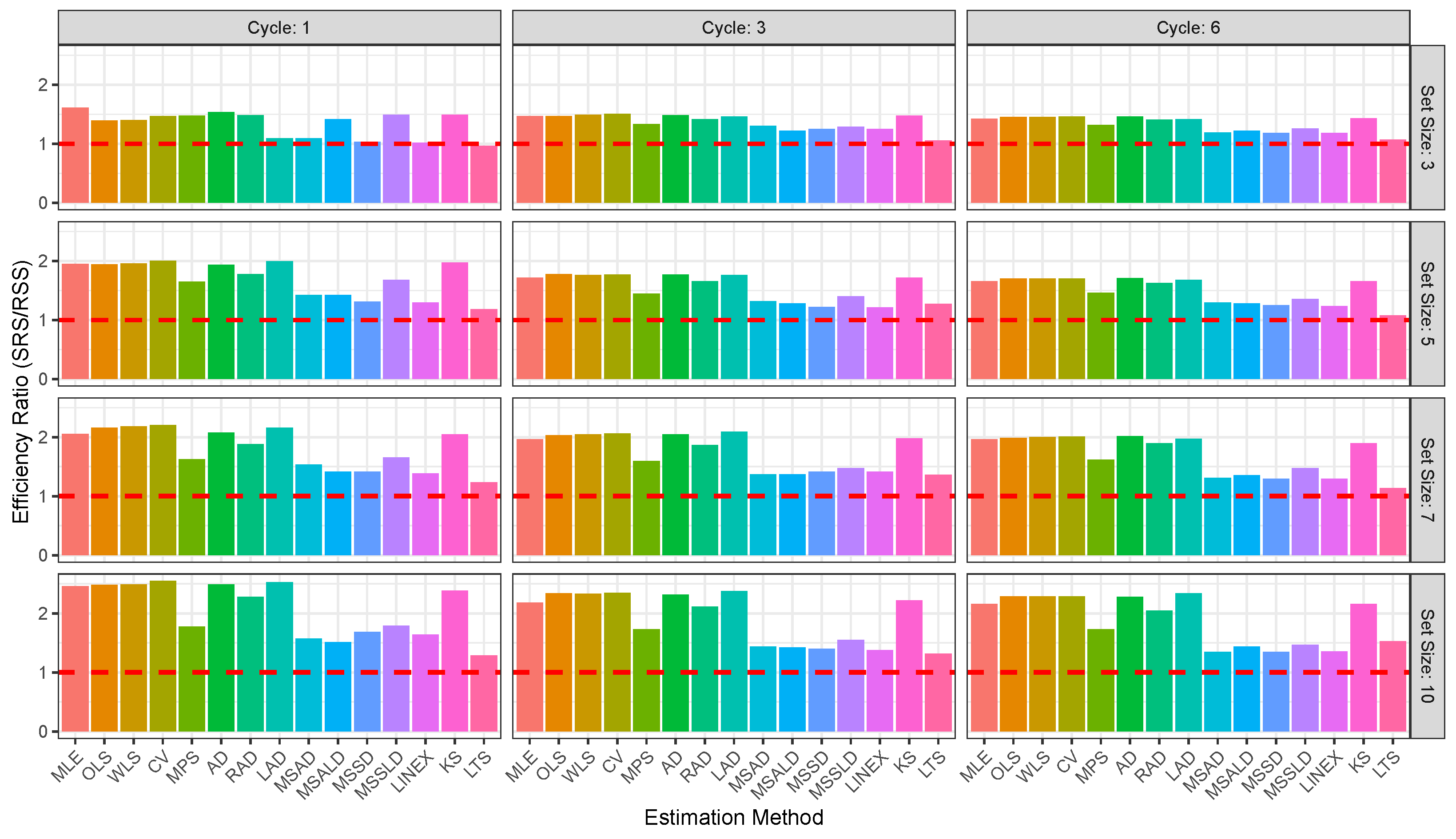
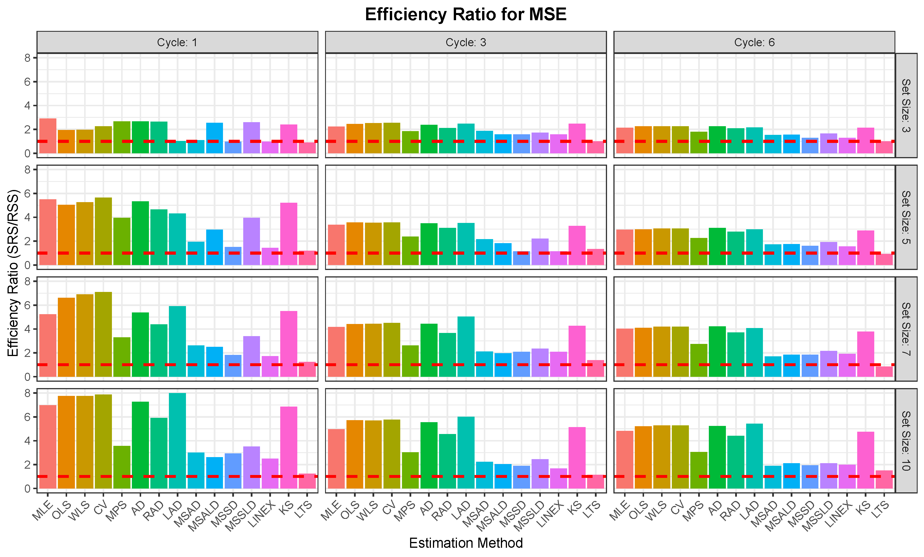
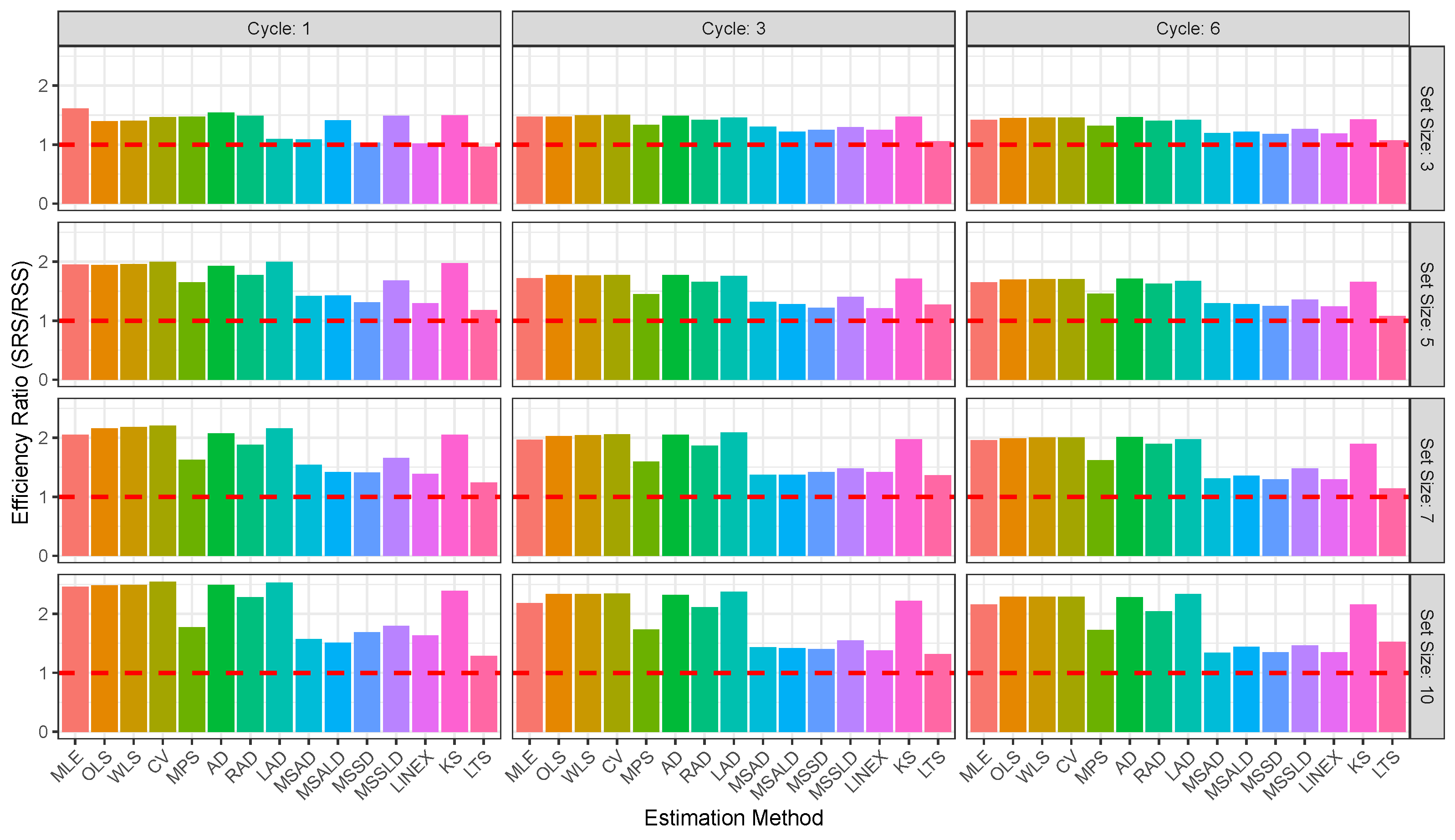
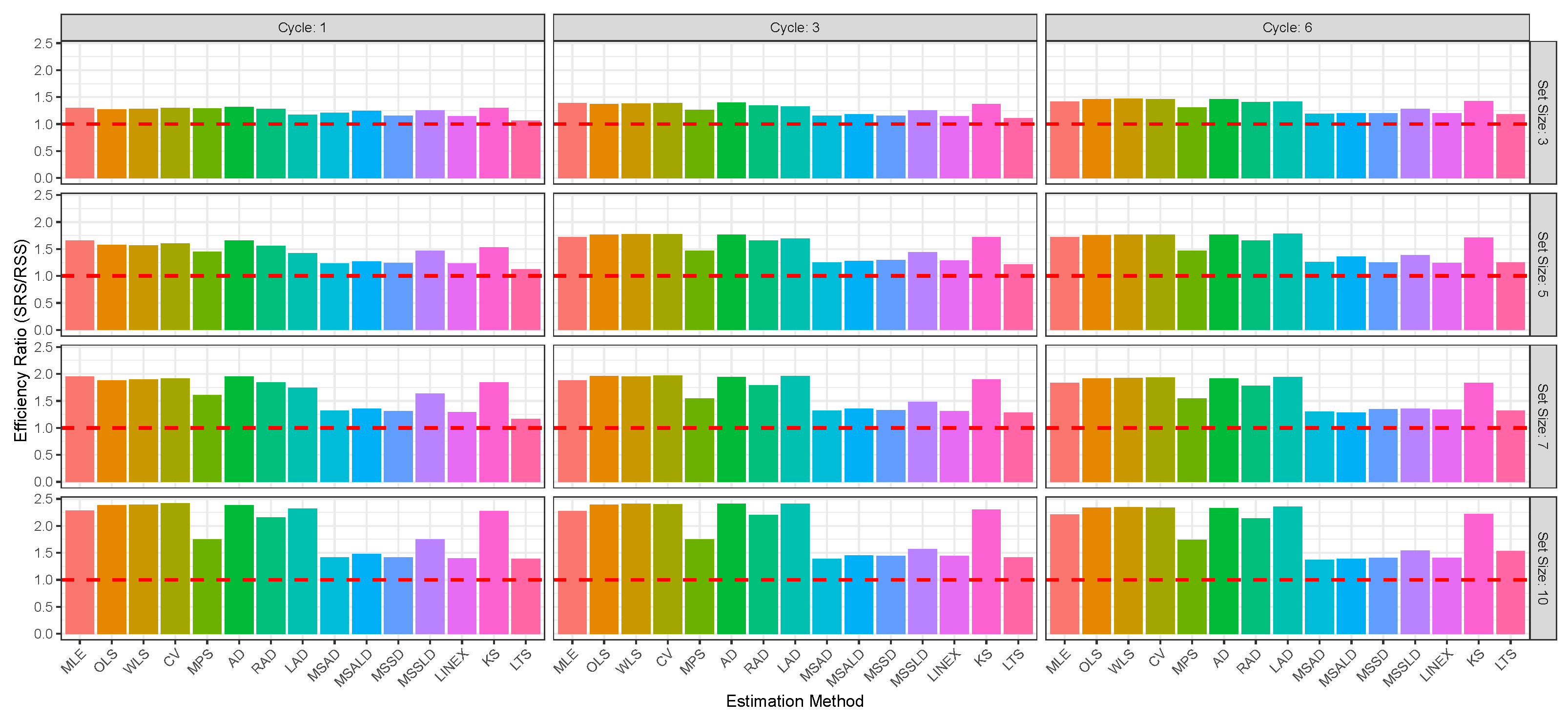
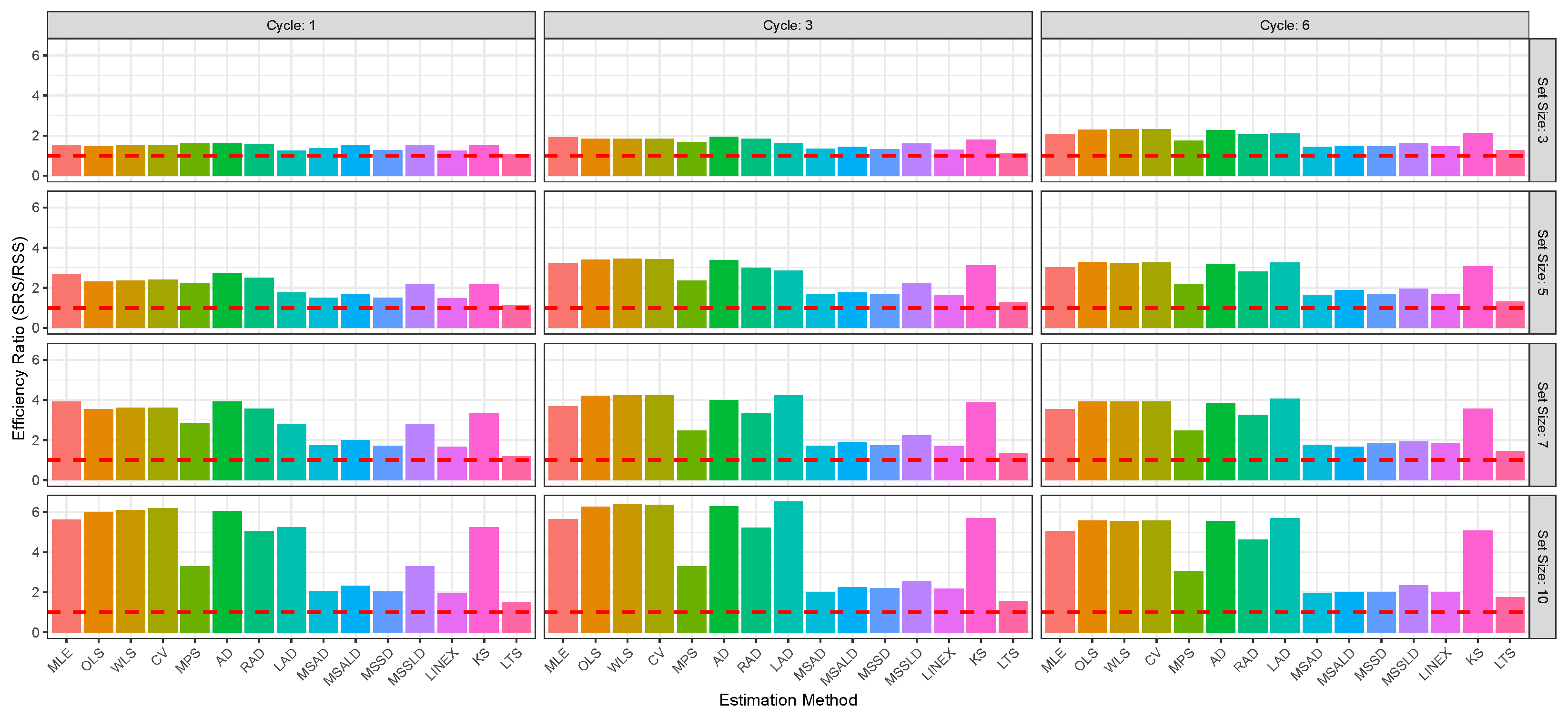
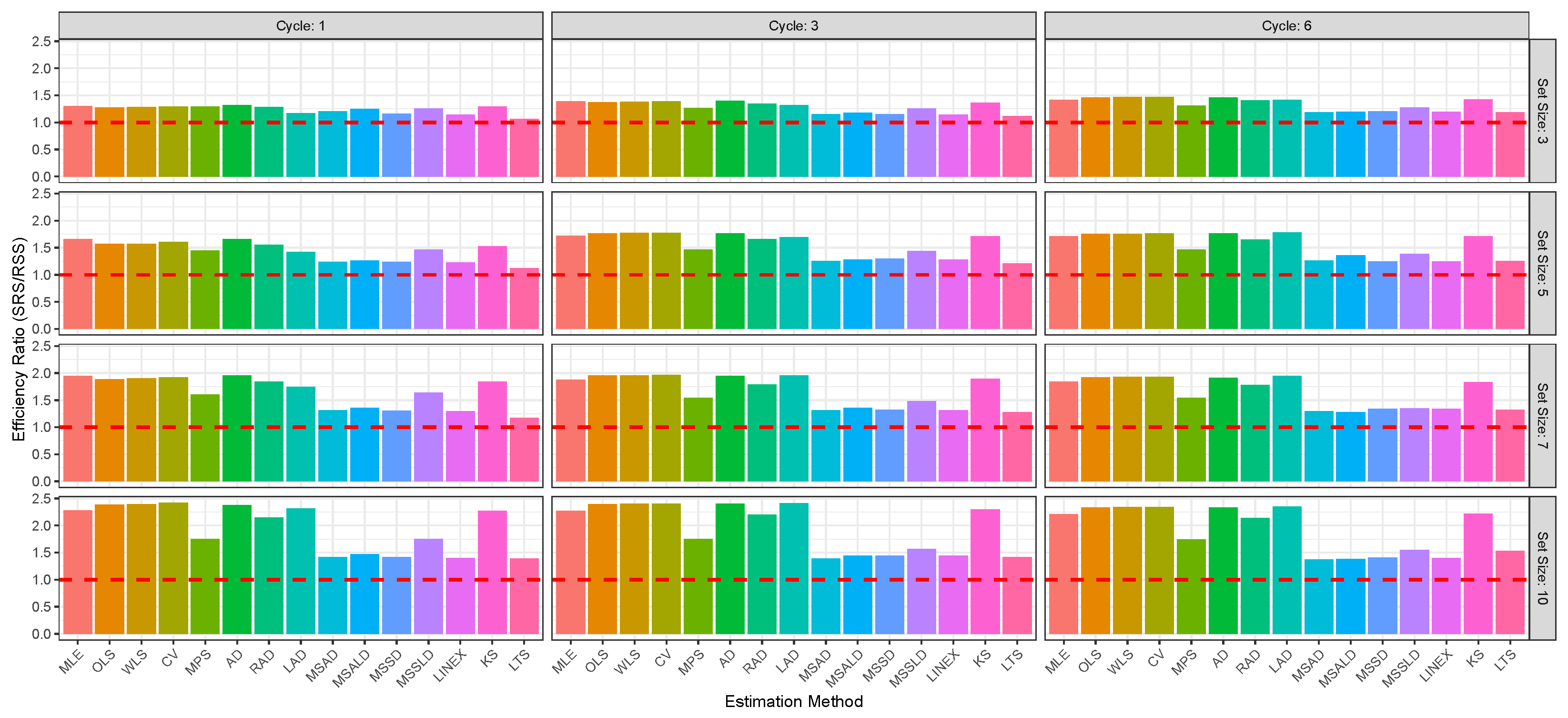
Figure 2, Figure 3, Figure 4, Figure 5, Figure 6 and Figure 7 enable direct comparison of estimation efficiency between SRS and RSS approaches. They display the efficiency ratios (ERs) between SRS and RSS which are calculated for the bias, MSE, and MRE as

$$ER({\Phi }_{RSS},{\Phi }_{SRS})={\displaystyle \frac{{\Phi }_{SRS}}{{\Phi }_{RSS}}},\Phi =\mathrm{Bias},\mathrm{MSE},\mathrm{MRE}.$$

For illustration of the reults given in Table 1, Table 2, Table 3 and Table 4, we consider three cases, namely the SRS with RSS, the parameter values based on SRS, and finally the effect of parameter values using RSS.

Table 1 and Table 2 aim to compare the RSS and SRS based on a simulation study for $\psi =2$. The following observations can be concluded:

• The RSS consistently outperforms SRS across the 15 estimation methods, MLE, OLS, WLS, CV, MPS, AD, RAD, LAD, MSAD, MSALD, MSSD, MSSLD, LINEX, KS, LTS, and various sample sizes, delivering mean estimates closer to the true value of $\psi =2$, with lower bias, MSE, and MRE. For illustration:

  ⇒

  The RSS produces estimators closest to parameter $\psi =2$ than SRS; for example, at $n=3$, ${\widehat{\psi }}_{MLE}^{RSS}=2.2791$ vs. ${\widehat{\psi }}_{MLE}^{SRS}=2.6148$, and at $n=60$, ${\widehat{\psi }}_{MLE}^{RSS}=2.0056$ vs. ${\widehat{\psi }}_{MLE}^{SRS}=2.0237$.

  ⇒

  Also, RSS exhibits lower bias across all methods and sizes; e.g., at $n=15$, $Bias\left({\widehat{\psi }}_{MLE}^{RSS}\right)=0.2050$ vs. $Bias\left({\widehat{\psi }}_{MLE}^{SRS}\right)=0.3520$, and at $n=42$, $Bias\left({\widehat{\psi }}_{MLE}^{RSS}\right)=0.1060$ vs. $Bias\left({\widehat{\psi }}_{MLE}^{RSS}\right)=0.2080$.

  ⇒

  Additionally, RSS achieves lower MSE, indicating better precision; e.g., at $n=18$, $MSE\left({\widehat{\psi }}_{MLE}^{RSS}\right)=0.0825$ vs. $MSE\left({\widehat{\psi }}_{MLE}^{SRS}\right)=0.1764$, and at $n=30$, $MSE\left({\widehat{\psi }}_{MLE}^{RSS}\right)=0.0189$ $MSE\left({\widehat{\psi }}_{MLE}^{SRS}\right)=0.0938$.

  ⇒

  The RSS shows smaller relative errors; e.g., at $n=5$, $MRE\left({\widehat{\psi }}_{MLE}^{RSS}\right)=0.1867$ vs. $MRE\left({\widehat{\psi }}_{MLE}^{SRS}\right)=0.3638$, and at $n=60$, $MRE\left({\widehat{\psi }}_{MLE}^{RSS}\right)=0.0385$ vs. $MRE\left({\widehat{\psi }}_{MLE}^{SRS}\right)=0.0830$.

• Based on different estimation methods:

  ⇒

  MLE: RSS excels, e.g., $n=3$ $Bias\left({\widehat{\psi }}_{MLE}^{RSS}\right)=0.6573$, with MSE of 0.9807 vs. $Bias\left({\widehat{\psi }}_{MLE}^{SRS}\right)=1.0585$, with MSE value 2.8469; and for $n=60$ $Bias\left({\widehat{\psi }}_{MLE}^{RSS}\right)=0.0769$, vs. $Bias\left({\widehat{\psi }}_{MLE}^{RSS}\right)=0.1660$, with respective MSE values 0.0093 and 0.0450.

  ⇒

  OLS: RSS outperforms, e.g., $n=15$ $Bias\left({\widehat{\psi }}_{OLS}^{RSS}\right)=0.2199$, with MSE of 0.0794 vs. $Bias\left({\widehat{\psi }}_{OLS}^{SRS}\right)=0.3906$, with MSE value 0.2823.

  ⇒

  MPS: RSS shines, often closest to 2, e.g., $n=18$ ${\widehat{\psi }}_{MPS}^{RSS}=1.9298$, with MSE of 0.0827 vs. ${\widehat{\psi }}_{MPS}^{SRS}=1.9597$, with MSE value 0.1495.

  ⇒

  LAD: RSS reduces larger errors, e.g., $n=21$ $Bias\left({\widehat{\psi }}_{LAD}^{RSS}\right)=0.1778$, with MSE of 0.0526 vs. $Bias\left({\widehat{\psi }}_{LAD}^{SRS}\right)=0.3716$, with MSE value 0.2650.

  ⇒

  LTS: RSS mitigates poor performance, e.g., $n=10$ $Bias\left({\widehat{\psi }}_{LTS}^{RSS}\right)=0.9824$, MSE = 4.3108 vs. $Bias\left({\widehat{\psi }}_{LTS}^{SRS}\right)=1.2664$ with MSE = 5.3731.

• Based on the sample size impact, the RSS’s advantage is most notable in smaller samples. For example:

  ⇒

  When $n=3$, the MSE of the MLE is 0.9807 vs. SRS 2.8469, which narrows slightly in moderate sizes.

  ⇒

  For $n=21$, MSE of the MLE = 0.0353 vs. that based on the SRS 0.1468,

  ⇒

  and it persists in larger sizes; for $n=60$ the MLE has MSE = 0.0093 vs. the 0.0450 MSE of SRS.

Based on Table 1 and Table 3 regarding parameter values, $\psi =2$ (Table 1) and $\psi =5$ (Table 3) under SRS design, one can see, in summary, that the results for $\psi =2$ generally exhibit lower absolute bias and MSE, making them better in terms of raw accuracy and precision. However, we have the following specific comments:

• The estimates in both tables tend to overestimate the true $\psi$, with values consistently above 2 and 5, respectively. This overestimation is more pronounced in absolute terms for $\psi =5$ due to the larger true value.
• Absolute bias is higher for $\psi =5$ than for $\psi =2$ across all methods and sample sizes. This is expected, as the same estimation error results in a larger deviation when the true value is 5 compared to 2. For instance, MPS has a bias of 0.8790 for $\psi =2$ vs. 1.9816 for $\psi =5$ at $n=3$.
• MSE is consistently higher for $\psi =5$ than for $\psi =2$, reflecting the larger scale of errors when estimating a true value of 5. For example, MPS has an MSE of 1.8264 for $\psi =2$ vs. 5.9552 for $\psi =5$ at $3n=3$, and 0.0427 vs. 0.3321 at $n=60$.
• MRE provides a normalized measure of error and shows mixed results. For small sample sizes (e.g., $n=3$), MRE is lower for $\psi =5$ (e.g., 0.3963 vs. 0.4395 for MPS), indicating better relative accuracy. For larger sample sizes (e.g., $n=60$), MRE is slightly lower for $\psi =2$ (e.g., 0.0824 vs. 0.0926 for MPS), suggesting a slight advantage in relative terms as sample size increases.
• As sample size n increases from $n=3$ to $n=60$, both bias and MSE decrease significantly for $\psi =2$ and $\psi =5$, indicating improved accuracy and precision with larger samples.

Utilizing the RSS method when $\psi =2$ in Table 1 and $\psi =5$ in Table 4, smaller $\psi$ values lead to more stable and accurate estimation, and it is noted the following general trends:

• As $\psi$ increases from 2 to 5, both bias and MSE increase for most estimators. This suggests that larger values of $\psi$ introduce more variability in estimation, making the estimation problem more challenging.
• Increasing the sample size helps reduce the impact of larger $\psi$, leading to lower bias and MSE. However, for $\psi =5$, larger sample sizes are even more crucial to maintain estimation accuracy.

5. Real Data Analysis

To evaluate the effectiveness of the proposed estimation strategies, we chose two real-world datasets and performed a detailed analysis in this section. Our goal was to highlight potential applications and situations where these techniques can be successfully implemented. By carefully analyzing real-world data, this study highlights the practical significance of these estimation methods, demonstrating their relevance for applied research and data-driven decision-making. To compare the estimators, and to verify that our U-LD model provides a good fit for the dataset under study, we conduct a Kolmogorov–Smirnov (KS_t) test, Anderson–Darling (AD_t) test, and a Cramér–von Mises (CV_t) test based on both SRS and RSS for all estimation methods considered in this study.

First Dataset: The first dataset under consideration consists of 20 items tested simultaneously, with their ordered failure times previously reported in [44]. The observed ordered data are as follows (

Table 5. Failure times data set.

0.0009	0.0040	0.0142	0.0221	0.0261	0.0418	0.0473	0.0834	0.1091	0.1252
0.1404	0.1498	0.1750	0.2031	0.2099	0.2168	0.2918	0.3465	0.4035	0.6143

).

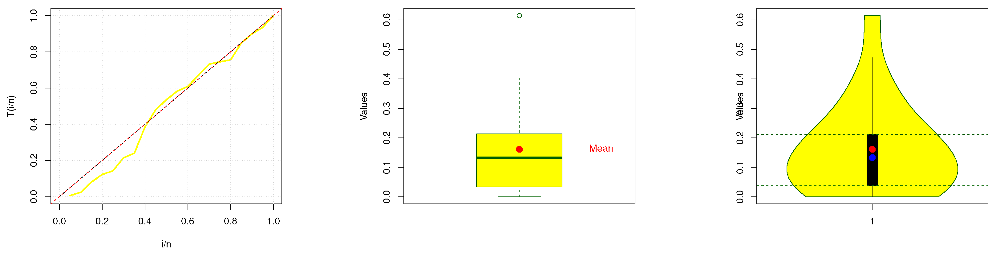
A descriptive statistics to the data is given in

Table 6. Descriptive statistics of failure times data set.

Measure	Value	Measure	Value
Count	20	Skewness	1.4406
Mean	0.1613	Kurtosis	2.3473
Standard Deviation	0.1573	Variance	0.0248
Min	0.0009	Range	0.6134
25th Percentile (Q1)	0.0379	Median	0.1328
75th Percentile (Q3)	0.2116	Max	0.6143

, which shows that the skewness of the dataset is approximately 1.44, indicating that the distribution is positively skewed. Since the median is 0.1328, it means that $50\%$ of the data points fall below this value, and a standard deviation of 0.1573 suggests that most of the data points are fairly spread out from the mean, with a decent level of variability.

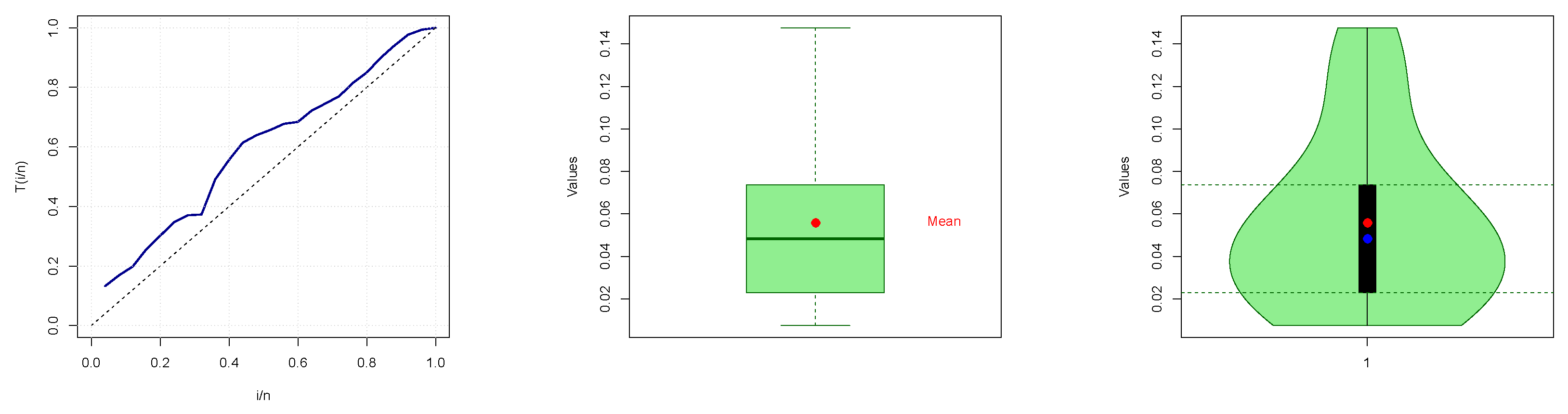
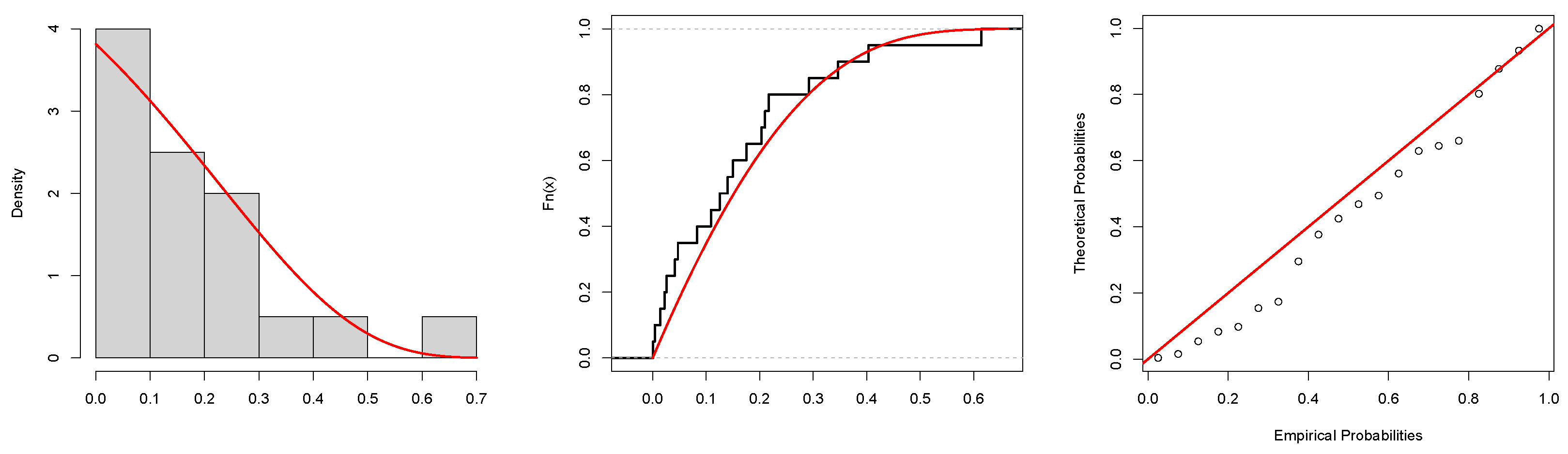
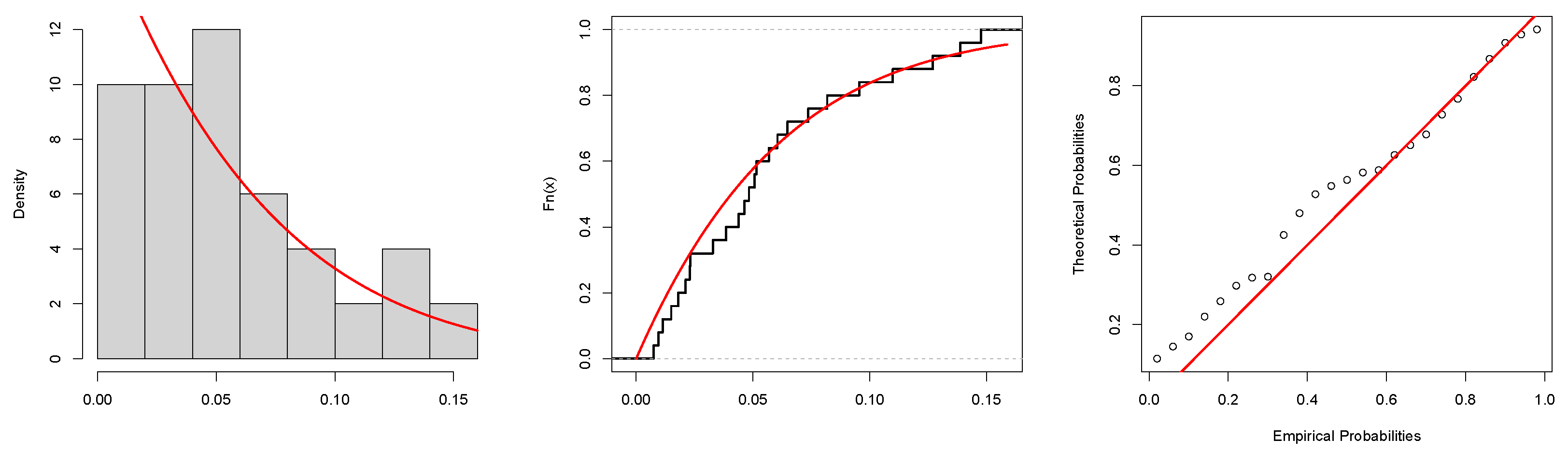
Also, Figure 8 presents graphical representations of the dataset, including the total time on test (TTT) plot, box plot, and violin plot. The estimated PDF, CDF, and probability–probability (PP) plots for failure times data are presented in Figure 9. These visualizations offer valuable insights into the dataset’s characteristics, facilitating a deeper understanding of its structure and trends.

Based on these data, we select a small RSS of size 4 while using the same sample size for the SRS. It is important to note that the SRS and RSS methods are compared using the same number of measured units. Using these methods, we estimate $\psi$ for each design, assuming perfect ranking. The results are summarized in

Table 7. Estimates and test statistics for each method under the two sampling schemes, SRS and RSS.

Method	$\widehat{\mathit{\psi }}$		ADt		CVt		KSt		p-Value
	SRS	RSS	SRS	RSS	SRS	RSS	SRS	RSS	SRS	RSS
MLE	4.0625	4.6153	1.6689	1.0820	0.2387	0.1271	0.1999	0.3533	0.1777	0.4977
OLS	3.7068	4.1552	2.2621	1.5446	0.3509	0.2151	0.2365	0.1812	0.1961	0.3756
WLS	3.6522	4.1274	2.3713	1.5806	0.3715	0.2219	0.2429	0.1593	0.1973	0.3689
CV	3.7972	4.2924	2.0926	1.3808	0.3188	0.1841	0.2261	0.2217	0.1906	0.4102
MPS	3.3812	3.9615	2.9957	1.8178	0.4894	0.2669	0.2760	0.0773	0.2078	0.3090
AD	3.7767	4.3021	2.1298	1.3702	0.3259	0.1820	0.2285	0.2121	0.1902	0.4127
RAD	3.8087	4.4255	2.0719	1.2437	0.3149	0.1580	0.2248	0.2273	0.1853	0.4453
LAD	3.7288	4.1240	2.2196	1.5851	0.3429	0.2228	0.2340	0.1906	0.1974	0.3680
MSAD	2.9853	3.6931	4.2025	2.2891	0.7156	0.3560	0.3284	0.0202	0.2381	0.1755
MSALD	2.9853	3.6931	4.2025	2.2891	0.7156	0.3560	0.3284	0.0202	0.2381	0.1755
MSSD	3.3266	3.9238	3.1397	1.8773	0.5165	0.2781	0.2829	0.0657	0.2120	0.2874
MSSLD	3.4081	3.9793	2.9273	1.7905	0.4765	0.2617	0.2726	0.0836	0.2059	0.3194
LINEX	3.3295	3.9212	3.1318	1.8814	0.5150	0.2789	0.2826	0.0662	0.2122	0.2860
KS	3.8434	4.1866	2.0112	1.5050	0.3034	0.2076	0.2209	0.2445	0.1949	0.3834
LTS	3.6067	3.8887	2.4663	1.9345	0.3895	0.2889	0.2483	0.1425	0.2158	0.2682

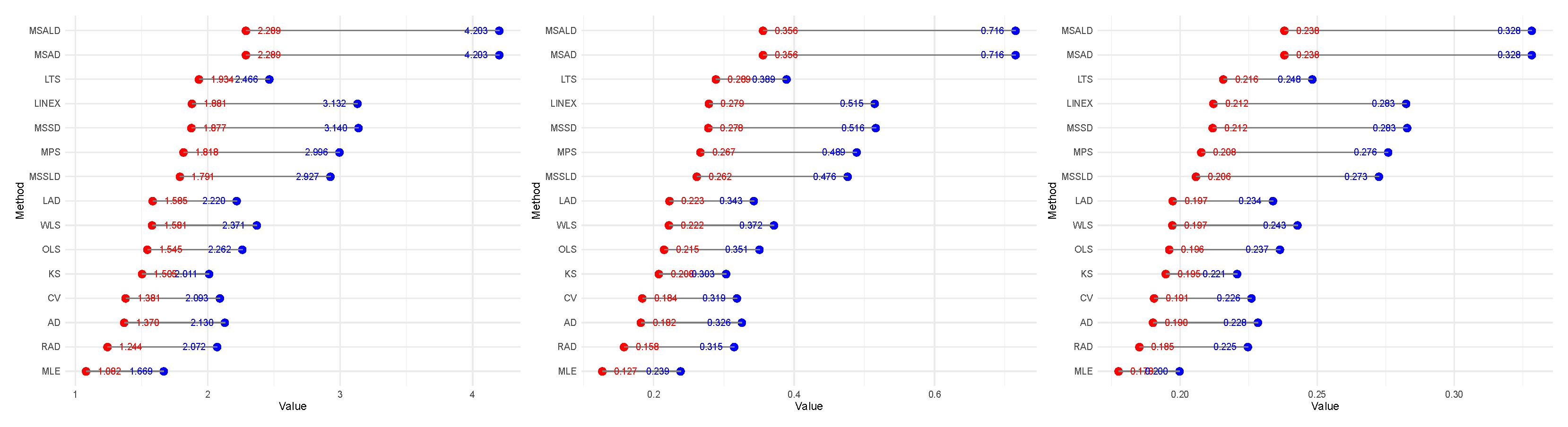
, indicating that the U-LD model fits the data well, as supported by various plots. For instance, for the OLS method based on RSS, the KS_t value is 0.1812 with a p-value of 0.3756. The Anderson–Darling test yields a value of 2.2621 using SRS, while the Cramér–von Mises test result is 0.2151 in RSS. These findings collectively support the adequacy of our model in fitting the dataset. Figure 10 further reinforces this conclusion, where blue dots represent SRS values, red dots red dots represent RSS values. Table 7 highlights the superiority of RSS over SRS in estimating the distribution parameter. For illustration, based on the MSALD, the AD_t values are 4.2025 and 2.2891 using SRS and RSS, respectively.

Second Dataset: The second dataset pertains to Turkey, which documented its first COVID-19 patient recovery on 26 March 2020 according to the World Health Organization (WHO). This dataset contains 25 observations of g collected from 27 March through 20 April. It was subsequently analyzed in study [45]. The chronologically ordered observations are as follows (

Table 8. COVID-19 recovery rates in Turkey.

0.0074	0.0095	0.0113	0.0150	0.0180	0.0212	0.0229	0.0231	0.0328	0.0385
0.0439	0.0464	0.0483	0.0507	0.0515	0.0568	0.0605	0.0648	0.0737	0.0818
0.0955	0.1099	0.1270	0.1388	0.1476

).

Descriptive statistics of the COVID-19 data are presented in

Table 9. Descriptive statistics of COVID-19 recovery rates in Turkey.

Measure	Value	Measure	Value
Count	25	Skewness	0.9213
Mean	0.0559	Kurtosis	0.0116
Standard Deviation	0.0409	Variance	0.0248
Min	0.0074	Range	0.1402
25th Percentile (Q1)	0.0229	Median	0.0483
75th Percentile (Q3)	0.0737	Max	0.1476

, revealing that the data are right-skewed with a skewness value of 0.91213. The COVID-19 data are illustrated using the TTT plot, box plot, and violin plot as shown in Figure 11, and the estimated PDF, CDF, and PP plots are offered in Figure 12.

Again, based on COVID-19 data, the estimators considered are compared and the U-LD model is fitted using the Kolmogorov–Smirnov test, the Anderson–Darling test, and the Cramér–von Mises test for both RSS and SRS across all estimation methods in this study. The results are summarized in

Table 10. Estimates and test statistics for each method under the two sampling schemes SRS and RSS for Dataset 2.

Method	$\widehat{\mathit{\psi }}$		ADt		CVt		KSt		p-Value
	SRS	RSS	SRS	RSS	SRS	RSS	SRS	RSS	SRS	RSS
MLE	12.1022	18.227	1.2534	0.7877	0.2164	0.1288	0.18	0.1481	0.3501	0.5917
OLS	9.8961	15.8023	2.7955	0.5036	0.5539	0.0641	0.2554	0.1049	0.0632	0.9194
WLS	9.9546	16.2165	2.7395	0.5176	0.5415	0.0682	0.2533	0.1077	0.0669	0.9044
CV	10.2278	16.9157	2.4903	0.5755	0.4865	0.0822	0.2434	0.1201	0.0867	0.8219
MPS	10.382	16.6771	2.3583	0.5511	0.4574	0.0765	0.2378	0.1149	0.0996	0.8594
AD	10.2546	16.7356	2.4669	0.5566	0.4814	0.0778	0.2424	0.1162	0.0888	0.8505
RAD	11.0187	17.2586	1.8751	0.6185	0.3513	0.092	0.2156	0.1276	0.1685	0.7638
LAD	9.3167	15.9451	3.4048	0.5067	0.6884	0.0651	0.2772	0.1059	0.0344	0.9144
MSAD	8.6666	17.8727	4.2189	0.718	0.868	0.1138	0.3026	0.1407	0.0158	0.6543
MSALD	8.6666	17.8727	4.2189	0.718	0.868	0.1138	0.3026	0.1407	0.0158	0.6543
MSSD	9.7655	14.439	2.9241	0.5792	0.5823	0.0761	0.2603	0.1115	0.0555	0.8812
MSSLD	11.2584	17.332	1.7171	0.6289	0.3168	0.0943	0.2075	0.1292	0.2015	0.751
LINEX	9.7611	14.2168	2.9285	0.6111	0.5832	0.0822	0.2604	0.1176	0.0552	0.8405
KS	9.7519	15.6017	2.9378	0.5027	0.5853	0.0633	0.2608	0.1036	0.0547	0.9262
LTS	8.261	15.1246	4.8068	0.5166	0.9971	0.0648	0.319	0.1004	0.0092	0.941

, while Figure 13 presents the values of the AD_t, CV_t, and KS_t measures, where blue dots represent SRS and red dots represent RSS. The findings indicate that the U-LD model fits the data accurately, as supported by various plots. For clarification, in the LTS method based on RSS, the KS_t value is 0.1004 with a p-value of 0.9410. The Anderson–Darling test value is 0.5166, while the Cramér–von Mises test result is 0.0648. Regarding the comparison between SRS and RSS, Table 10 highlights the superiority of RSS over SRS in estimating the distribution parameter across all cases. For instance, based on the MSSD method, the KS values are 0.2603 and 0.1115, with corresponding p-values of 0.0555 and 0.8812 for SRS and RSS, respectively.

However, in general, it is important to emphasize that the RSS design exhibits superior efficiency compared to the SRS design, as evidenced by its smaller goodness-of-fit values. This consistent advantage of RSS over SRS is observed across all estimates. These findings highlight the benefits of using the RSS approach over SRS for fitting the dataset to the model and obtaining more efficient estimates.

6. Conclusions

This paper thoroughly investigates various estimation methods for the parameter of the U-LD under both RSS and SRS designs. A wide range of estimation techniques is explored, including maximum likelihood estimation, ordinary least squares, weighted least squares, maximum product of spacings, minimum spacing absolute distance, minimum spacing absolute log-distance, minimum spacing square distance, minimum spacing square log-distance, linear-exponential, Anderson–Darling (AD), right-tail AD, left-tail AD, left-tail second order, Cramér–von Mises, and Kolmogorov–Smirnov. The simulation study performed as part of this research shows that the estimators derived from RSS consistently outperform those derived from SRS across all the criteria considered: mean squared error, bias, and efficiency. This suggests that RSS provides more reliable and efficient parameter estimates when applied to the U-LD distribution. Additionally, the analysis of two real-world datasets, failure times of items, and COVID-19 data demonstrates the practical applicability of the proposed estimation methods. The findings clearly highlight the advantages of using RSS over SRS for statistical inference, particularly in the context of U-LD parameter estimation. In conclusion, this study underscores the superiority of RSS-based estimators in parameter estimation for the U-LD distribution. The results emphasize the importance of considering the sampling design when choosing appropriate estimation methods and recommend RSS as a preferable choice for enhanced statistical inference in various practical applications. Further research could explore the robustness of these findings under different sampling schemes and distributional assumptions.