Abstract
The dynamic study of current and rapid movements of rigid and multibody mechanical systems, according to differential principles from dynamics, is based on advanced concepts from analytical mechanics: kinetic energy, higher-order acceleration energies, and their absolute time derivatives. In advanced dynamics, the study will extend to higher-order acceleration energies. This paper, reflecting the authors’ research, presents new and revised formulations in advanced kinematics and dynamics, with a focus on acceleration energies of the higher order. Explicit and matrix representations of the defining expressions for higher-order acceleration energies, relevant to the current and rapid movements of rigid bodies and multibody mechanical systems, are presented. These formulations include higher-order absolute time derivatives of advanced concepts, following the specific equations from analytical dynamics. Based on the authors’ findings, acceleration energies play a central, decisive role in formulating higher-order differential equations, which describe both rapid and transient motion behavior in rigid and multibody systems.
Keywords:
mechanics; analytical dynamics; kinetic energy; acceleration energies; advanced dynamic equations; robotics MSC:
70E55
1. Introduction
Analytical mechanics, based on the principles established by Lagrange and Hamilton, provides a fundamental basis for describing the motion of rigid and multibody systems. The traditional formulations usually rely on first- and second-order derivatives of motion parameters. However, in modern applications such as high-speed robotics, aerospace engineering, and advanced control mechanisms, higher-order acceleration terms are essential for describing dynamic behaviors, particularly in transient and rapid motion conditions.
To address these challenges, researchers have extended analytical mechanics by integrating higher-order acceleration energies for improving the precision of dynamic models. For example, Miron investigated Lagrangian and Hamiltonian geometry, offering a geometric basis for higher-order formulations [1]. Additionally, Levi-Civita and Lanczos contributed significantly to the development of mathematical methods used in classical mechanics [2,3]. The inclusion of higher-order acceleration terms has significantly improved motion prediction and control in fields such as robotics and aerospace engineering, where systems are subjected to rapid accelerations and transient motions.
Following recent developments in this area, the authors have also developed theoretical approaches in the field of advanced analytical mechanics. This research is focused on refining the energy of acceleration formulations and extending dynamic equations to include higher-order derivatives, which are essential for accurately modeling complex mechanical systems [4,5].
Recent studies have further explored the role of higher-order kinematics in multibody dynamics and robotics. Thus, Mueller introduced a comprehensive framework for higher-order kinematics in lower-pair chains, focusing on their importance in mechanism theory and robotic applications [6]. Other researchers such as De Jong and Jonker developed a framework for the study of rigid body dynamics by introducing higher-order derivatives, improving their applicability to flexible multibody systems [7]. Moreover, research on screw and Lie group theory in multibody dynamics optimized the use of recursive algorithms for solving equations of motion in complex systems [8]. Lukierski et al. also studied acceleration-extended Galilean symmetries, demonstrating their significance in higher-order mechanics and physics-based models [9].
In a recent study, Condurache, D., introduced a method for analyzing higher-order acceleration fields in the motion of rigid bodies and multibody systems by applying the properties of nilpotent algebra. This interesting approach contributes to the development of advanced kinematic models that can be applied for complex mechanical systems, where higher-order effects are significant.
In accordance with the fundamental principles of analytical mechanics, this paper analyzes higher-order acceleration energies and differential principles that are essential for characterizing the dynamic behavior of complex mechanical systems.
Relevant to both robotics and mechanical engineering applications, the research addresses the requirements of systems that require precise motion control in complex mechanical systems. By introducing novel formulations in advanced kinematics and dynamics, the work extends the mathematical model to include higher-order derivatives and acceleration energies. This model offers a clearer perspective of rapid and transient motion phenomena, providing a more accurate approach for modeling complex mechanical behaviors. The primary goal is to develop explicit, matrix-based representations of higher-order acceleration energies, which are essential for the modeling and control of high-velocity mechanical systems. The research focuses on integrating these advanced dynamic formulations into differential equations that effectively characterize both static and dynamic phases in complex mechanical structures.
Additionally, the paper presents some novel contributions by introducing matrix representations to facilitate the mathematical description of higher-order kinematic and dynamic quantities. Furthermore, it develops explicit higher-order acceleration energy expressions and applies the proposed formulations to rigid bodies and multibody systems, demonstrating their effectiveness in modeling high-speed transient motions.
The paper examines key aspects from analytical mechanics and explores their implications for dynamic modeling and control of complex mechanical systems. The following sections present the theoretical model, mathematical derivations, and applications of higher-order acceleration energies in analytical mechanics.
2. Materials and Methods
This theoretical study focuses on the advanced development of kinematic and dynamic principles in analytical mechanics, specifically concerning higher-order acceleration energies and their applications in complex mechanical systems.
The approach is based on rigorous mathematical models and matrix formulations to extend existing theories [4,5]. This section outlines the theoretical framework, mathematical tools, and key equations employed in formulating higher-order dynamics for rigid and multibody systems, providing the foundation for the later analysis of dynamic behaviors under complex motion conditions.
2.1. Position and Orientation Parameters of Solid Body
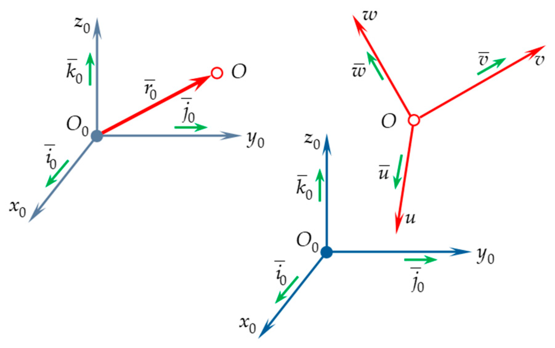
The solid body is a physical form of matter’s existence in the material universe. Consequently, the solid body is considered a material continuum. Based on this property to achieve an exact geometric solution, the solid body is decomposed into an infinite number of elementary particles, each with an infinitesimal mass and a continuous distribution throughout its geometric form. If the distances between the elementary particles are kept constant, the solid body will be characterized as a rigid solid (S). When density is consistently supported within the rigid structure, a homogeneous rigid solid is obtained. If the integration limits around the entire geometric contour are well defined, the homogeneous body will have a simple or regular geometric shape. In this case, geometric and mass integrals are applied. Before conducting the mechanical study (static, kinematic, and dynamic modeling), it is essential to show the geometric state of the rigid body at each moment of its movement in Cartesian space. To this end, the geometric state of the simplest mechanical model, the material point, is studied first (Figure 1). Based on research from [4,5,6], the following notations are introduced:

Figure 1.
Position and orientation parameters.
In Equation (1), the coordinates and axes of the Cartesian reference system are defined; in Equation (2), the unit vectors (versors) of the reference system axes are specified; and in Equation (3), the angles and direction cosines are defined.
Following Figure 1, the rigid body is subject to geometric study. For this purpose, two reference systems are considered: the first system, denoted as , is a fixed-reference system, and the second system, , is a moving-reference system, permanently attached to the body, with its origin at point , an arbitrary point on the rigid body. The reference system , also represented in Figure 1, is a system with its origin at point , whose orientation remains constant throughout the motion and is identical to that of the fixed-reference system, , meaning . The geometric state of any point belonging to the rigid body (for example, an arbitrary point ) represents its position, defined, according to Figure 1, by the following position vector:
For a free material point, the three linear coordinates defined in Equation (5) are independent and represent the degrees of freedom (d.o.f.). The study then extends to a vector or an axis belonging to the Cartesian reference system (Figure 1).
This geometric state is referred to as orientation (angular state). Orientation (angular state) is defined by using unit vectors. For any unit vector , assumed to be known in relation to one of the reference systems or , the orientation will be defined by means of the direction cosines.
In accordance with linear algebra, the symbol in Equation (6) defines the transpose of the matrix. Considering the second expression in Equation (6), it can be observed that the orientation of any vector or axis is defined by two independent angles. The geometric aspects presented earlier are examined in the context of an orthogonal, right-handed reference system (see Figure 1, ) relative to the fixed-reference system . In this case, the geometric state is represented by position and orientation. Position is defined by Equation (5) while orientation is defined by the rotation matrix [4,10,11,12,13,14]:
The resulting rotation matrix defined by Equation (7) contains the unit vectors of the reference system relative to the fixed-reference system . The rotation matrix, or direction cosine matrix, describes the orientation of each axis of the moving-reference system attached to the rigid body in relation to a fixed-reference system. Among the nine direction cosines in the rotation matrix, six mathematical relationships can be proved. Therefore, the orientation of a moving-reference system relative to a fixed-reference system can be defined by a maximum of three independent parameters, represented by the orientation angles. Consequently, the resulting orientation of a reference system relative to another reference system, or , can be defined by three independent orientation angles (degrees of freedom), according to [4,6]:
The angles included in Equation (8) are components of the orientation column matrix , which geometrically describe dihedral angles between two geometric planes:
Physically, the three angles defined by Equation (9) represent a simple rotation around one of the three axes of the Cartesian reference system: .
Based on the research in [4,6,15], combining these three simple rotations results in twelve sets of orientation angles (8). Considering , the expressions for the three simple rotation matrices are further developed as follows:
The following mathematical representation of the generalized rotation matrix is proposed:
Here,
and
By substituting Equations (13) and (14) into the generalized Equation (12), the simple rotation matrices defined in Equation (11) are obtained. The generalized matrix can thus be written as follows:
In Equation (15), the symbol defines the antisymmetric matrix associated with vector (17) while represents the diagonal matrix, determined as
The matrix (15) can also be defined by means of the following classical formulation:
According to the research [4,5], the three simple rotations defined by Equation (8) can be performed either around the fixed axes or the moving axes, belonging to the and / reference systems. The resulting rotation matrix, denoted as , which expresses the orientation of the reference system relative to fixed-reference system, is defined by expressions that also include matrix exponentials as follows:
Using the author’s research on matrix exponentials [16], the resulting rotation matrix can be expressed in a new form as follows:
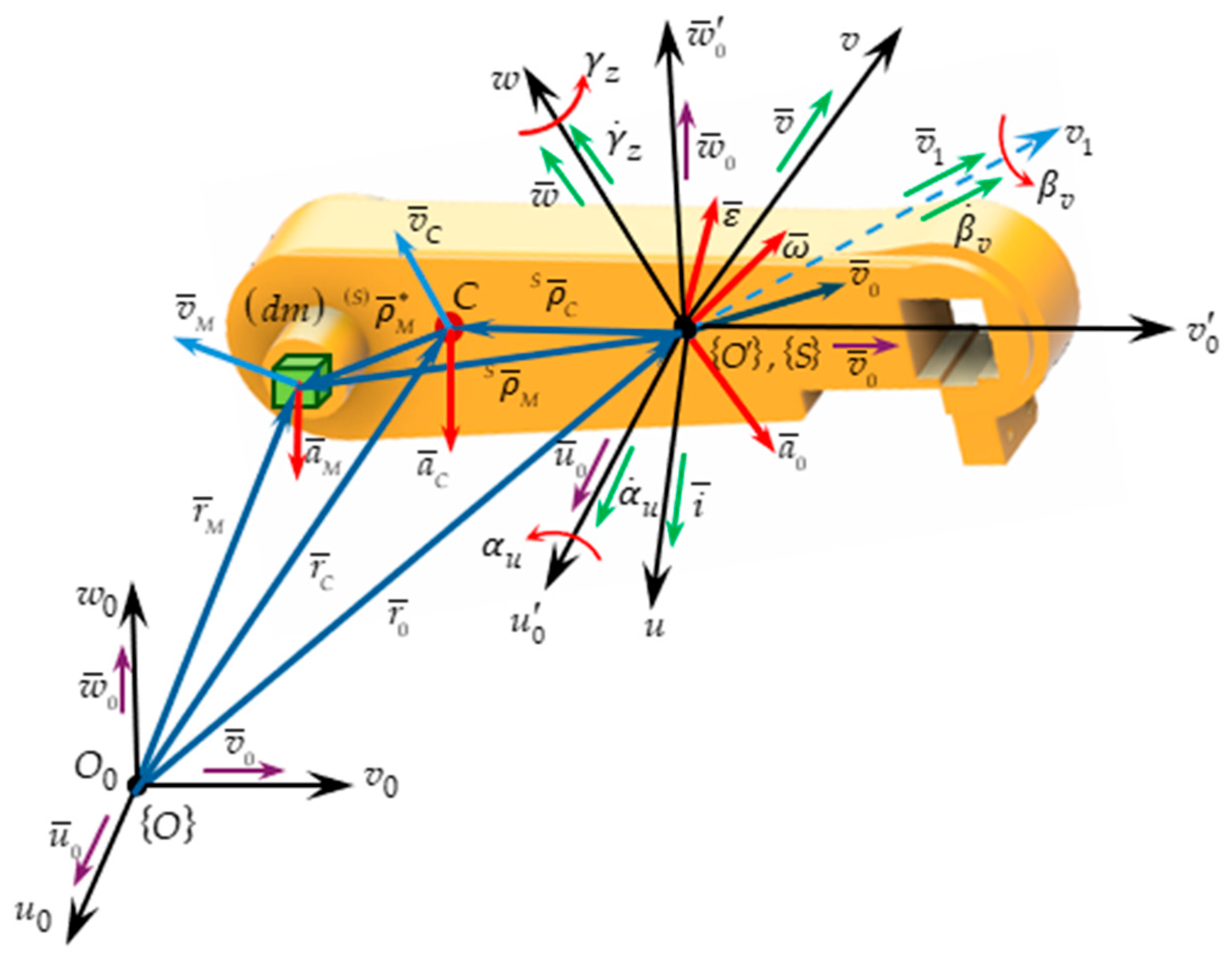
Equations (5) and (8), presented above, define the position and orientation of a right-handed reference system. These mathematical expressions will be generalized for the case of a rigid body. According to [5,11,17], a rigid body is composed of an infinite number of material particles and an infinite number of geometric axes, parallel and perpendicular to each other, characterized by a continuous distribution throughout the entire volume of the rigid body. The rigid body also includes an infinite number of sets consisting of three orthogonal geometric planes, continuously distributed throughout its volume. Geometrically, to define a right-handed reference system with its origin at an arbitrary point belonging to the rigid body, it is sufficient to select a single set composed of three orthogonal planes. According to Equation (4) and Figure 2, this reference system is denoted as . The reference system is attached to the rigid body. Equations (5) and (8) define the position and orientation of this system.
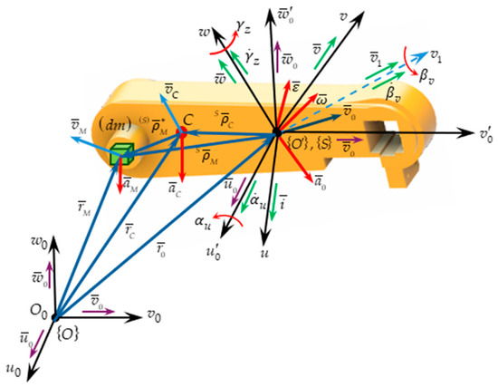
Figure 2.
Representation of a free rigid body in Cartesian space.
Since the purpose of this paper is to study advanced dynamics, two material points belonging to the rigid body are considered, satisfying the conditions and . The expressions defining the absolute position become time-dependent vector functions [4,5] as follows:
Considering Equations (23) and (25), the absolute position equation can be written using matrix exponentials [16] as follows:
The absolute position equation for any material point belonging to the rigid body can be determined when the position and the orientation of the moving system are known. Analyzing Equations (23) and (24) reveals that the orientation is invariant for all points of the rigid body. Based on these geometric considerations, the body is represented by the reference system . This system is geometrically defined by six independent parameters or degrees of freedom, included in the following symbol:
Here, and is the generalized coordinate; is an operator that highlights the type of degrees of freedom:
The symbols presented in Equation (28) define higher-order generalized variables in the case of rapid motions, where is the order of the time derivative.
In advanced mechanics, instead of Equation (8), the following definition is used for the angular orientation vector:
Here, is the angular transfer matrix, which is a matrix defined as a function of the orientation angles, and specified according to the expression below:
The position and orientation of the moving-reference system, relative to any other system, such as the fixed-reference system, can be represented in matrix form using transformations based on matrix exponentials:
Equation (32) defines the position vector of the moving system relative to the fixed system while Equation (34) represents a vector defined as a function of screw parameters (homogeneous coordinates).
Matrix formulation is widely used in multibody system’s kinematics and dynamics. The application of matrix exponentials in kinematic and dynamic modeling of complex systems offers advantages over classical transformations, including a compact representation of components and the ability to use computer calculus. Also, in the matrix exponential calculus, reference frames are avoided; these, in robot structures, are typically assigned based on specific geometric constraints (which may introduce geometric errors). This property of matrix exponentials is due to the presence of screw parameters in the exponential functions. The conclusion and defining expressions presented in this introductory section will be applied further in the study of advanced kinematics and dynamics of mechanical systems.
2.2. Significance of Higher-Order Derivatives in Analytical Dynamics
In analytical mechanics, higher-order derivatives are essential for accurately describing and predicting the motion of complex mechanical systems. While velocity and acceleration (first- and second-order derivatives) are often sufficient for basic applications, more advanced systems require additional motion analysis. Higher-order derivatives allow for a more precise understanding of motion, especially in systems that involve rapid changes, complex interactions, and precise control requirements.
One important reason for using higher-order derivatives is to improve motion accuracy. In fields such as robotics, aerospace engineering, and biomechanics, acceleration alone is not always enough to describe how a system moves. Additional derivatives, such as jerk (third order) and snap (fourth order), help create smoother and more controlled motion paths. This is particularly useful in systems where sudden changes in speed or direction must be carefully managed to avoid mechanical stress or instability.
Higher-order derivatives also play a key role in modeling transient motion situations, where acceleration changes abruptly. Many mechanical systems, such as robotic arms, vehicles during sudden breaking, or flexible structures under load, experience these rapid transitions. Standard acceleration-based models often fail to capture these changes correctly, leading to inaccurate simulations or inefficient control. By including higher-order terms, models can better represent real-world movement and improve the design of mechanical systems. Another major advantage of higher-order derivatives is their application in vibration control and shock absorption. In areas such as structural mechanics and material science, engineers use these derivatives to design systems that reduce excessive vibrations and improve stability.
This is especially important in precision manufacturing, vehicle suspension design, and energy-efficient mechanical systems, where smooth transitions between different motion states help optimize performance and durability. Despite these benefits, using higher-order derivatives comes with challenges. One of the biggest difficulties is the increased complexity of calculations.
While these derivatives improve model accuracy, they also require more advanced numerical methods, which can make computations more expensive and time-consuming.
Higher-order derivatives are a valuable tool in analytical mechanics. They help improve motion accuracy, enhance control, and provide a better understanding of complex movements. While they introduce computational and measurement challenges, their advantages outweigh these limitations, making them an important part of modern engineering and mechanical system design.
2.3. The Parameters of Advanced Mechanics
Based on the authors’ research, this section will present a series of new formulations about advanced kinematic concepts. A rigid body (S) represented in Figure 2 and undergoing general motion is considered. By applying the first-order absolute derivative to the parametric motion equations, we obtain the following:
According to [12,13,14,15,16,17], the antisymmetric matrix associated to angular vector is
Finally, expressions for linear velocities and accelerations are obtained in the form
The absolute position equation, expressed in terms of matrix exponential results, is
In advanced kinematics and dynamics, the higher-order derivatives applied to position vectors and rotation matrices are expressed as follows:
where
The defining expressions for angular velocities and accelerations can be proved based on matrix exponentials as follows:
Although the use of matrix exponentials may appear complex, it offers advantages, including the elimination of reference systems, which can impose certain restrictions.
This is evident in the previously presented equations by , showing that the unit vectors correspond to the initial state of the reference system . The position of the center of mass is found relative to the reference system as
The position of the mass center relative to reference system, at first in classical form and then in an exponential form, is presented:
If first- and second-order derivatives with respect to time are applied to Equation (44), the linear velocity and acceleration of the center of mass are ultimately obtained:
The absolute linear accelerations of higher orders, with respect to mass center, are as follows:
In dynamic modeling, the following expression is applied:
Using the author’s research [18] on time functions for position and orientation, the following differential properties have been developed in the study of advanced kinematics and dynamics of the rigid body, according to the following expressions:
Based on Equations (52)–(54), the expressions for a rigid body are obtained:
Here, .
Expressions (55) and (57) refer to the higher-order linear velocities and accelerations corresponding to the center of mass.
The other expressions, (56) and (58), define the higher-order angular velocities and accelerations specific to the rigid body in general motion.
The above expressions are also extended to multibody systems.
In case of rapid movements, higher-order operational and generalized accelerations develop within the mechanical structure (for example serial robot structures). Based on the research from [18,19], the following expressions are found:
Here, represents the order of differentiation with respect to time, the symbol is the column matrix of higher-order operational accelerations, and is the column matrix of higher-order generalized accelerations, defined according to the following:
Based on the mathematical models presented in [5], the Jacobian matrix can be found using matrix exponentials. Analyzing all input parameters in advanced kinematics reveals that they are functions of the generalized variables Equations (59) and (60) and their time derivatives.
Thus, following [18], these can be developed using polynomial interpolation functions. It is important to mention that in the kinematic and dynamic study of robotic structures, the application of higher-order polynomial functions is recommended as their reunion defines the so-called motion trajectories.
Depending on the working process in which the structures are implemented and the imposed constraints, these polynomial functions become motion functions, known for each degree of freedom of the analyzed structure.
This paper proposes the following higher-order polynomial functions:
On each trajectory segment , the number of unknowns is , and the meaning of the terms contained in (61) is as follows
Determining the unknowns in Equation (63) requires, in accordance with [8,9,10,11,12,13,14,15,16,17], the application of geometric and kinematic constraints:
The results of the polynomial interpolation functions Equation (61) will be substituted into the expressions defining the concepts of advanced kinematics and dynamics. Expressions for input data and higher-order parameters are essential in defining the concepts of advanced dynamics. In this work, these are represented by kinetic energy and higher-order acceleration energies. These concepts will be integrated into dynamic equations characterizing the rapid motions of bodies.
The aspects presented above provide essential advantages in the inverse dynamic study of robots. The drawback of these functions lies in their mathematical nature as approximative functions, requiring many trajectory intervals to achieve an approximate solution. For standard motions (without the occurrence of higher-order accelerations), these polynomial functions transform into cubic spline polynomial functions.
3. Discussion
3.1. Higher-Order Acceleration Energies
To understand the mechanical significance of higher-order energies, first, the expression of kinetic energy [5] is defined. Initially, a rigid body in general motion is considered (Figure 2). The starting equation for proving the kinetic energy of a rigid body is as follows:
A series of matrix transformations is performed on Equation (66). These are highlighted in the expressions presented below:
By substituting Equations (67) and (69) into Equation (68), the equation defining the kinetic energy in the case of general motion of the rigid body transforms into the following:
With the specific conditions: (Figure 2), Equation (70) becomes
Here, is the inertial tensor axial centrifugal versus .
Equation (71) represents König’s theorem for kinetic energy in its explicit form, characterizing general motion. In the case of multibody systems, the expression for König’s theorem is changed as follows:
The operator from Equation (73) has the following significance:
Considering [5], the total kinetic energy, in case of multibody systems, can be expressed using the rotational and translational components as follows:
The translational and rotational components are rewritten, following [4,5], considering the expressions of linear and angular velocities. They become the following:
In the equations of advanced dynamics, higher-order derivatives with respect to time are applied to kinetic energy. These expressions are as follows:
The theorem of kinetic energy in differential form includes the theorem of the motion of the center of mass (the impulse theorem) and the theorem of angular momentum with respect to the center of mass. Consequently, it is the most general fundamental theorem of Newtonian dynamics. The differential equation of this theorem is represented by the following:
By replacing the real differentiation operator (d) with the virtual differentiation operator (δ), Equation (78) becomes the generalization of d’Alembert–Lagrange’s principle.
As mentioned in [5], this theorem includes the differential expression of kinetic energy and mechanical work. Consequently, the kinetic energy theorem (79) will be written in a new mathematical form. For holonomic multibody systems, the following constraints are applied to Equations (78) and (79):
These conditions are applied to the independent parameters of finite and elementary displacements. Applying the differential transformations, the result is obtained:
Based on the author’s research [5,18,19], in the context of multibody systems, Equation (81) represents the generalized Lagrange’s equations of the first kind in analytical dynamics. Here, the term ‘advanced concepts in analytical dynamics’ refers to motion-related energies, whose primary components are higher-order accelerations. These accelerations are relevant especially for mechanical systems undergoing rapid or transient movements.
Starting from Appell’s function—introduced in 1899 and known as the kinetic energy of accelerations [14]—the author developed new formulations for first-, second-, third-, and fourth-order acceleration energies [18].
The expressions for acceleration energies were defined in the case of a rigid body and then for multibody systems. According to [18], the expression for acceleration energy corresponding to a rigid body in general motion was proven. With the square of the elementary mass acceleration as its central function, this type of energy, named the first-order acceleration energy, is defined as follows:
Here,
By expanding the mass integral (83), the first three terms are established:
The next three components are dedicated to generalized rotation. Of these, the first two hold angular velocity and angular acceleration. The defining expressions are as follows:
The components contained in Equation (88) are explained below:
Substituting the Equations (89)–(95) into Equation (88), the following expression results:
The last part, corresponding to rotational motion, exclusively holds the angular velocity vector, as can be seen in the expression below:
The integrand from the mass integral (97) is further expanded as follows:
The function (102) is substituted in Equation (97) resulting in the following expression:
By substituting Equations (84)–(89), (96), and (104) into Equation (83), the first-order acceleration energy in explicit form, for a rigid body in general motion, is obtained:
Introducing the conditions: (Figure 2), Equation (105) becomes the following:
In the case of multibody mechanical systems, the acceleration energies of the order and their time derivatives of order have the following starting expression:
Equation (107) contains the planar centrifugal inertia tensor, relative to the system:
For multibody mechanical systems, the acceleration energy of first order becomes:
Considering the concepts presented in [18], the two components (translational and rotational) of the first-order acceleration energy can be expressed as functions of higher-order accelerations as follows:
According to the literature, in multibody systems undergoing rapid or transient motions, as well as in mechanical systems subjected to external forces characterized by a time-varying law, higher-order linear and angular accelerations arise. Thus, the authors developed the second-order acceleration energy, with the following mass integral as the starting equation for a rigid body:
For multibody mechanical systems, the following explicit expression [5,11,13] for the second-order acceleration energy is introduced:
The study extends to the third-order acceleration energy, with the mass integral as the starting equation for a rigid body:
In the case of multibody systems, the acceleration energy of the third order becomes:
Based on [5,18], the study extends to the fourth-order acceleration energy, with the mass integral as the starting equation for a rigid body:
For multibody mechanical systems, the fourth-order acceleration energy becomes a central function , and the defining expression is presented below:
Taking (107) into account, the nth order acceleration energy can be established, whose general expression, according to [5,18], is presented below:
The objective of this section was to provide a detailed derivation of the general form of first-order acceleration energies, which are specific to general motion and consist of two main components: translational and rotational.
We have also demonstrated the equations for acceleration energies by considering higher-order derivatives of generalized variables. However, due to the complexity of calculations for other types of acceleration energies, we have limited our presentation to their definition expressions.
From the author’s perspective, acceleration energies could be physically interpreted as the time rate of change of mechanical power. According to the author’s research, higher-order acceleration energies become central functions of higher-order differential expressions specific to both rapid motions as well as the transient motion regimes of rigid bodies and multibody mechanical systems.
3.2. The Equations of Advanced Dynamics
Unlike classical mathematical models in analytical mechanics, such as the d’Alembert–Lagrange equations, second-kind Lagrange equations, or Hamilton’s equations, the explicit and matrix-form mathematical models presented in this paper are considered new models that provide an alternative approach to solving complex aspects of current and rapid motion dynamics.
In the Gibbs–Appell equations, developed in 1899, the first-order acceleration energy is used as the central function for holonomic and nonholonomic mechanical systems. These equations yield the same results as the second-order Lagrange equations, which are based on kinetic energy. In this work, the authors extend the study to rapid motions, where higher-order accelerations play a significant role. From a dynamic perspective, these accelerations become key components of what the authors define as higher-order acceleration energies. These equations lead to second-order differential equations, which describe typical motions where accelerations remain below . As a result, by applying higher-order derivatives to the Lagrange and Gibbs–Appell equations, the paper derives differential equations of motion that explicitly incorporate higher-order acceleration energies.
For mechanical systems (MBSs) dominated by sudden movements and transient motions, based on the research from [5,18], the theoretical and experimental existence of higher-order acceleration energy is proven. The expressions of acceleration energies are substituted into the higher-order differential equations of analytical dynamics. Consequently, the time variations of the generalized forces, which express the dynamic behavior of the multibody systems, become clear. Thus, considering the aspects from [4,18], the generalized inertia forces are derived with respect to time, resulting in the following expressions:
Here, is the order of differentiation with respect to time.
By considering the differential principle in its generalized form, Equation (81), the generalized inertia force becomes thus:
According to Lagrange equations of the second type, the generalized inertia force is as follows:
Here, Equation (127) represents Mangeron’s formulation and is the order of differentiation with respect to time. Based on first-order acceleration energy [5,18] and higher-order derivatives, the generalized inertia force is also identical to the following:
According to [18], Equation (128) represents the generalization of the Gibbs–Appell equations. Considering [18,19,20,21], the higher-order differential equations of motion have been presented. The first, second, and third absolute derivatives are applied to Equations (124) and (125). By several transformations, the expressions become the following:
Here, ,
The higher-order-dynamics Equations (130)–(132) contain higher-order acceleration energies, the definitions of which are presented according to [5,18].
The author proposed, in [5,18], generalized higher-order differential equations corresponding to MBS systems with rapid and transient motions:
The necessary conditions from expression (134) are as follows:
In various works by the main author, generalized expressions in explicit and matrix form have been presented for energies of acceleration and higher-order dynamics equations.
The mathematical models proposed in this paper, whether in explicit or matrix form, are generalized models that lead to second-order and higher-order differential motion equations (canonical equations) for any type of mechanical system motion: general motion, simple or resultant rotational motion, or movements specific to robotic structures (serial, parallel, or mobile).
3.3. Motivation in Using Higher-Order Acceleration Energies
Higher-order acceleration energies play a key role in accurately describing the motion of complex mechanical systems, particularly in applications where rapid transitions, high-speed dynamics, and precision control are required. While traditional models based on velocity and acceleration provide a solid foundation for motion analysis, they often fail to fully capture the effects of abrupt changes in acceleration, vibrations, and dynamic instabilities. By incorporating higher-order derivatives, such as jerk and snap, it is possible to achieve smoother transitions, improve system stability, and enhance predictive accuracy in real-world applications.
One of the main reasons for using higher-order acceleration energies is to ensure smooth motion transitions, especially in robotic systems, autonomous vehicles, and aerospace applications. When acceleration changes suddenly, it can introduce mechanical stress, vibrations, and instability. By considering higher-order terms, control algorithms can generate motion trajectories that minimize abrupt force variations, improving both efficiency and durability. In robotics, for instance, smooth trajectory planning helps reduce wear on mechanical components and ensures greater precision in positioning. Similarly, in autonomous vehicles, incorporating higher-order derivatives leads to smoother breaking and turning maneuvers, enhancing both passenger comfort and vehicle stability. Another important aspect is the role of higher-order acceleration energies in structural integrity and vibration control. Mechanical systems subjected to frequent acceleration changes, such as high-speed trains, aircraft landing gear, or flexible structures, experience fatigue over time. Excessive jerk and snap can lead to unwanted oscillations, reducing the lifespan of components and affecting overall system performance. By integrating higher-order terms into dynamic models, engineers can develop structures that better absorb shocks, minimize vibrations, and distribute loads more effectively, ultimately improving safety and efficiency.
Beyond mechanical applications, higher-order acceleration energies are also essential in computational modeling and numerical simulations. In crash testing, aerospace trajectory simulations, and precision engineering, incorporating higher-order derivatives allows for more accurate predictions of how forces propagate through a system. This leads to better material selection, improved structural designs, and enhanced real-time control capabilities. Moreover, in applications requiring vibration damping, such as precision manufacturing or satellite stabilization, higher-order motion modeling helps develop advanced control systems that reduce disturbances and maintain system accuracy.
Overall, the use of higher-order acceleration energies is motivated by the need for greater accuracy, stability, and efficiency in dynamic systems. Whether in robotics, vehicle dynamics, aerospace engineering, or structural mechanics, their inclusion enables better motion control, reduces mechanical stress, and enhances predictive modeling. While their implementation may introduce computational challenges, the benefits in terms of system performance and longevity make them essential tools in modern analytical mechanics.
4. Application of Acceleration Energies and Dynamic Equations
In the following section, a practical application that demonstrates the use of a mathematical model based on acceleration energies is presented.
The main objective is to show how theoretical principles related to acceleration energies are applied to real-world engineering scenarios. To make the concepts more accessible, we have selected a case study focused on the rotational motion of the arm of a serial robot, namely Fanuc LR Mate 100 iB (see Figure 3). This is a compact 5-degree of freedom serial manipulator that is commonly used in different industrial applications such as high-speed pick and place, assembly, or material handling. It is characterized by lightweight structure and a low payload capacity that makes it ideal for educational and research activities involving motion, analysis, and control.
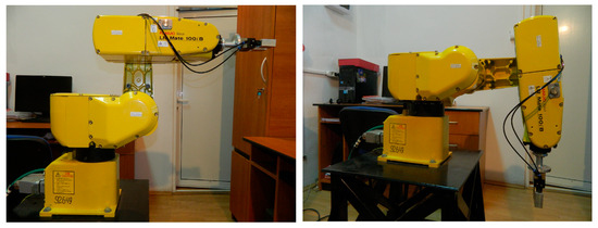
Figure 3.
The Fanuc robot used during the experiments.
The case study presented in the paper was carried out over an angular interval of (0, π), with a total motion duration of 1.7 s. Due to the complexity of the calculation procedures, this paper presents only the essential steps and most relevant results that are important for clarifying the key aspects of the proposed mathematical model.
To highlight the time-dependent behavior of higher-order acceleration energies, fifth-order polynomial interpolation functions were applied by considering the relevant kinematic constraints. Experimental measurements were carried out using a mono-axial accelerometer mounted on the third kinetic ensemble of the robot arm. This setup enabled the acquisition of tangential acceleration values at the characteristic point. These values were recorded every 0.033 s during the high-speed rotation of the robotic arm.
The collected data were used to generate graphical representations of both the tangential acceleration (as shown in Figure 4) and the generalized angular acceleration over the analyzed interval. Additionally, to capture the robot’s behavior under sudden stop conditions, similar measurements were repeated and visualized, offering a more comprehensive view of the arm’s dynamic response.
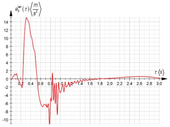
Figure 4.
Time variation in tangential acceleration during high-speed motion.
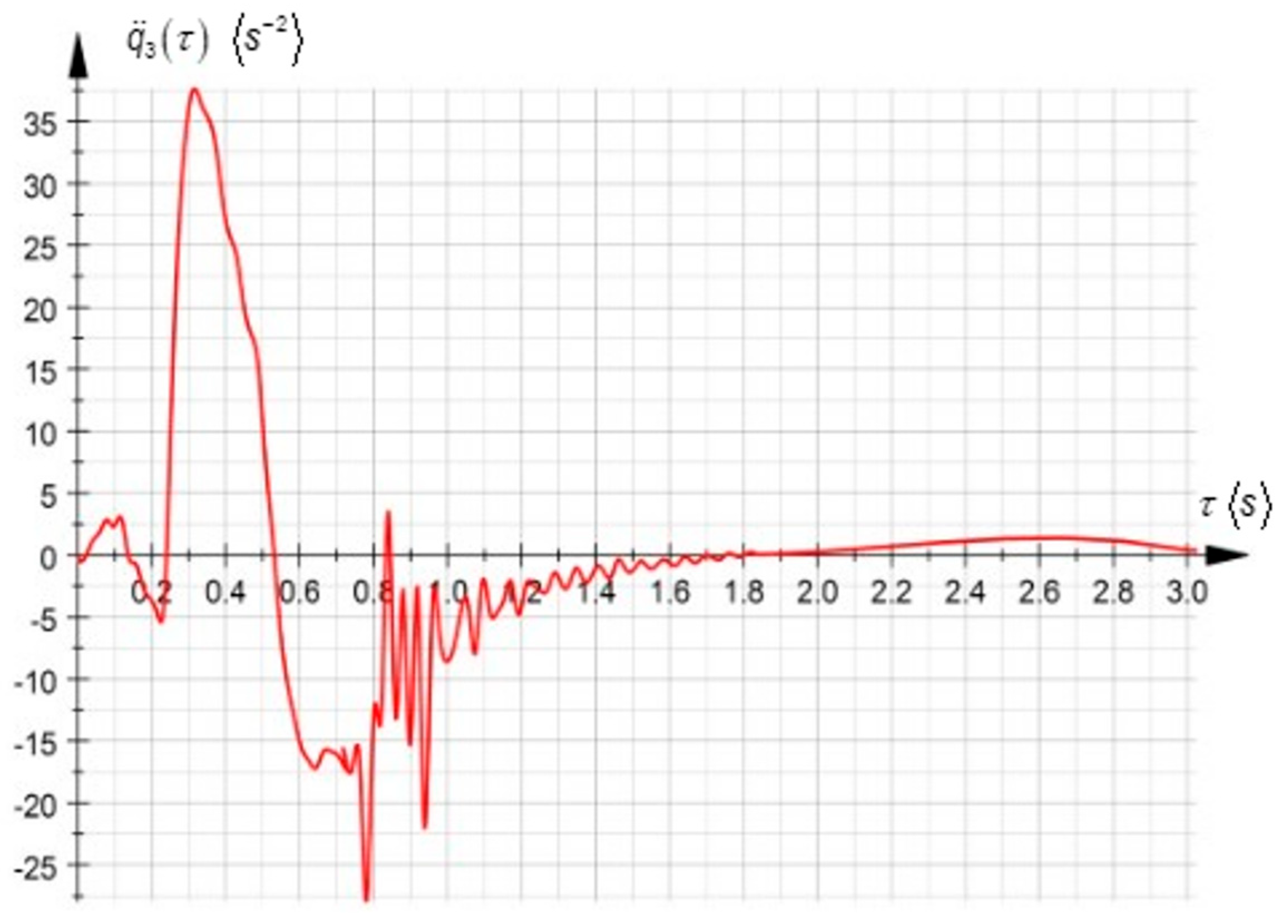
In this application, the fifth-degree polynomial interpolation functions for a real-time variable were used. Their expressions were obtained by particularizing Equations (61) and (62), previously presented in the paper. To determine the integration constants, the numerical values of the angular accelerations (as shown in Figure 5) were substituted into polynomial functions. By applying geometric and kinematic constraints specific to the work process, polynomial functions were obtained for all the 51 trajectory segments considered in the analysis, with a total duration of 1.7 s. As an example, for the trajectory segment considered within the time interval [0.565, 0.605], the corresponding interpolation functions were obtained, as presented below:

Figure 5.
Time variation in angular acceleration of first order during high-speed rotation.
By using Equations (110), (117) and (118) or by particularizing Equation (122) for , the first-, second- and third-order acceleration energies were obtained:
Furthermore, the application of Equations (130)–(132)—or the particularization of expression (134) for —representing the derivation order, led to the analytical expressions of the first-, second-, and third-order driving torques acting on the driving axis of the robotic arm. These expressions are presented below as follows:
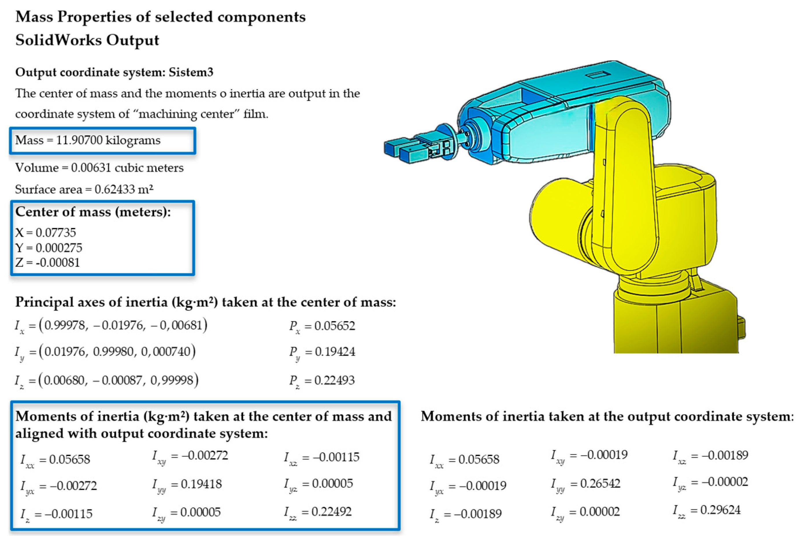
In Equations (141)–(146) the symbols denote the masses of the analyzed kinetic link of the Fanuc LR Mate 100 iB industrial robot (Figure 6).
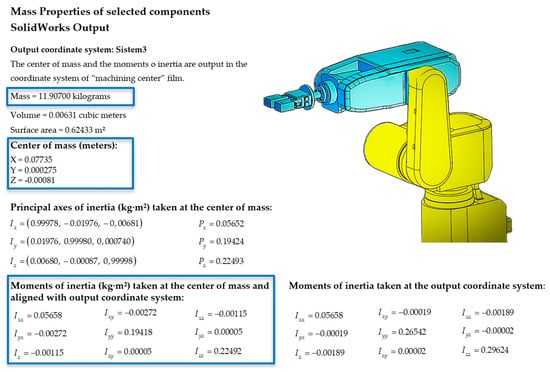
Figure 6.
Extract from SolidWorks: numerical values for mass, center of mass coordinates, and inertia tensors. The blue boxes indicate the most relevant parameters for dynamic analysis.
Correspondingly, , and , where , represent the mechanical moment of inertia of these links relative to their local coordinate axes .
The parameters and indicate the spatial coordinates of the center of mass for the third kinetic element. These mass properties were obtained using SolidWorks 2022 (Dassault Systèmes, Vélizy-Villacoublay, France) environment based on 3D models of robot components and are illustrated in Figure 6. The use of SolidWorks allowed the precise determination of geometric and inertia data, essential for the dynamic modeling of the robot structure.
In the context of this paper, the mass properties served as input data for the analytical formulation of the acceleration energies and driving torques of a higher order. The integration of these physical characteristics ensured consistency between the theoretical model and the real mechanical structure of the robot. By assigning real values to these quantities, the dynamic behavior of each kinematic link could be evaluated, which is essential for the validation of the proposed mathematical model.
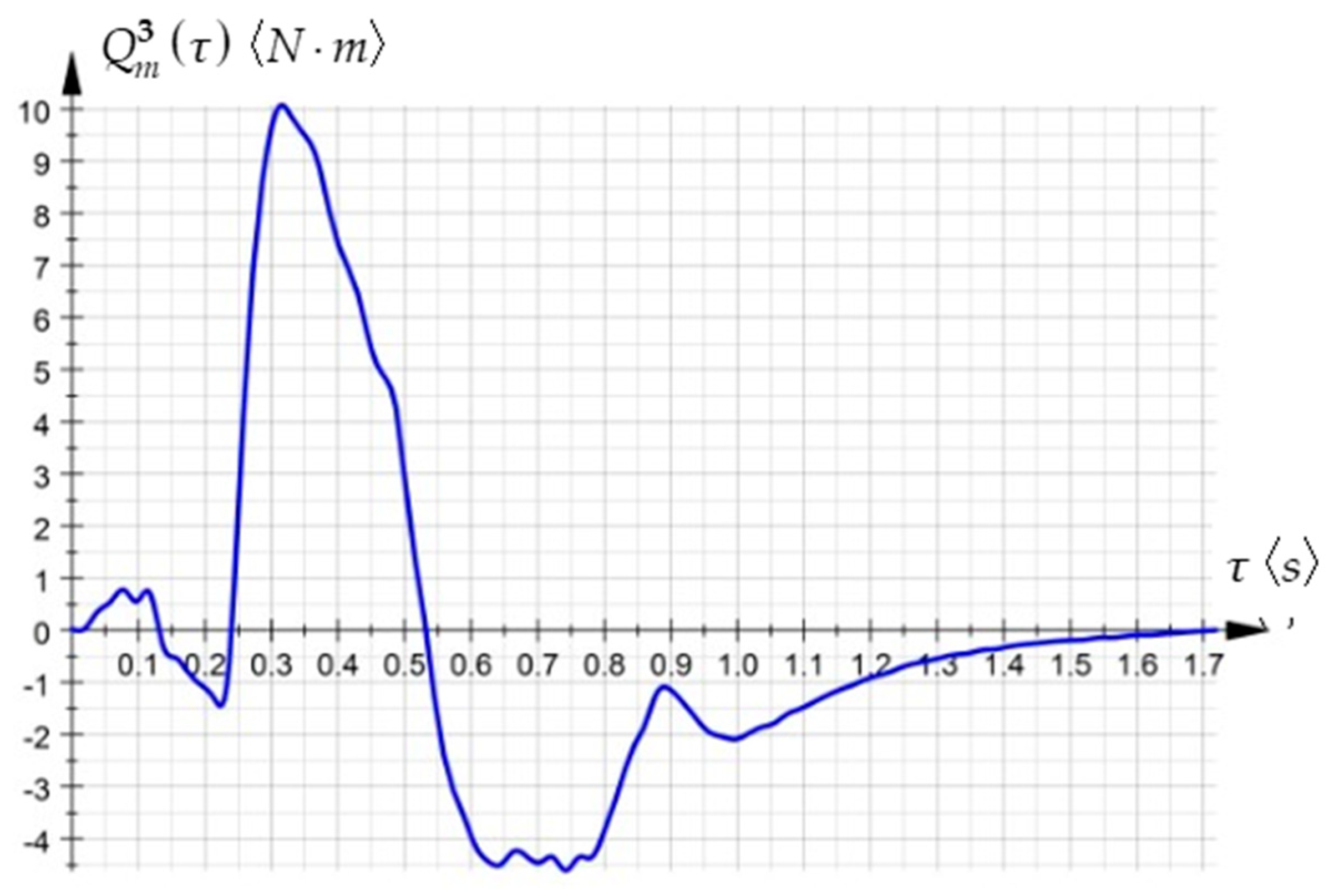
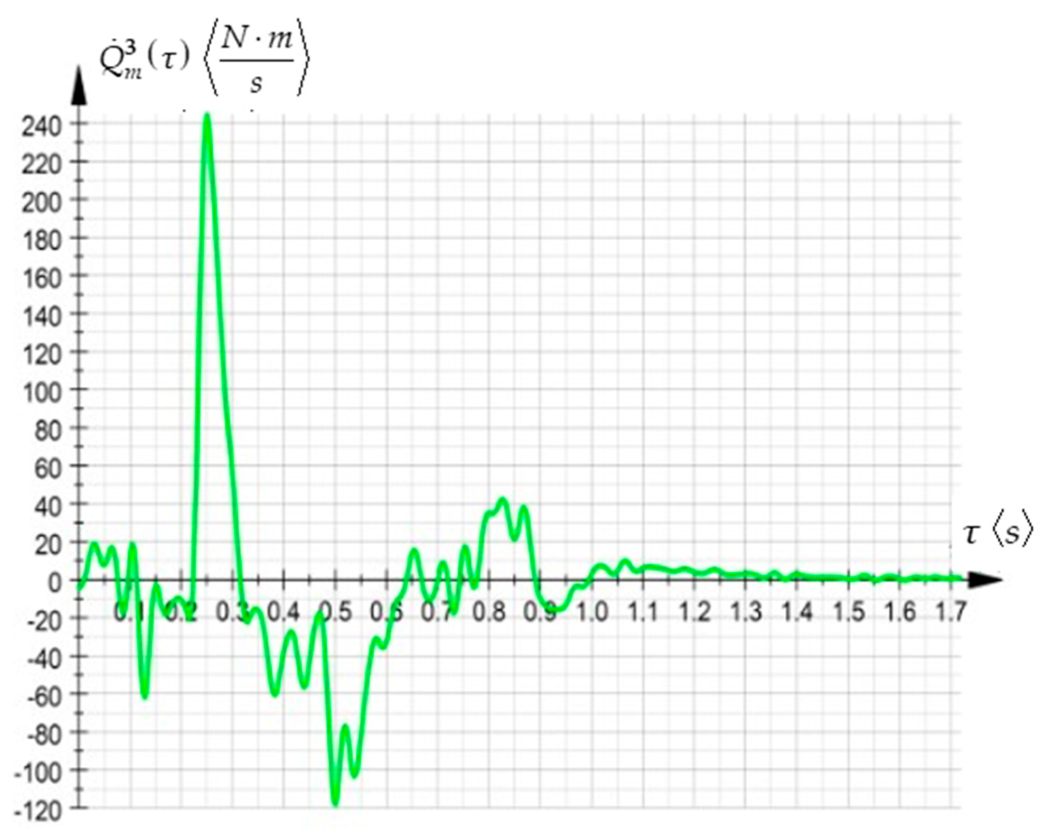
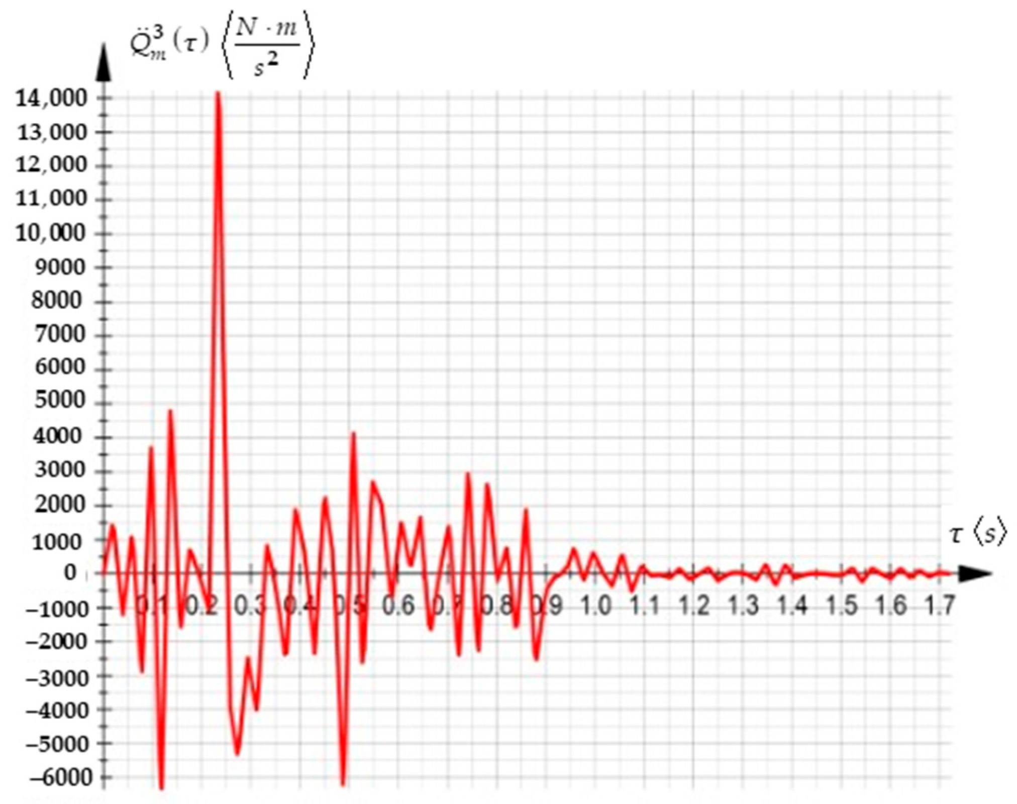
Further, the polynomial functions characterizing the entire work process were substituted into the analytical expressions, resulting in the time variations of the torque and its first- and second-order time derivatives, as illustrated in Figure 7, Figure 8 and Figure 9:

Figure 7.
The time variation in the torque.
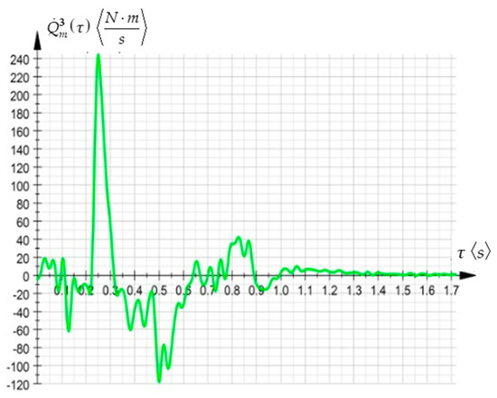
Figure 8.
The time variation law of the first-order time derivative of the torque.

Figure 9.
The time variation law of the second-order time derivative of the torque.
The above graphical representations illustrate, for the considered application, the time variation in the driving torque in the rotation axis of the robotic arm, whose expressions implicitly included the first-, second- and third-order acceleration energies.
5. Conclusions
The dynamic study of current and rapid motions of rigid bodies and multibody mechanical systems, following the differential principles characterizing system dynamics, is based on advanced concepts from analytical mechanics, namely kinetic energy, higher-order acceleration energies, and their absolute derivatives with respect to time. These advanced concepts are found in direct connection with the generalized variables or independent parameters corresponding to holonomic mechanical systems. The expressions of these advanced notions hold, on one hand, the kinematic parameters and their differential transformations corresponding to absolute motion, and on the other, the properties of masses. Considering the authors’ research, this work presents reformulations and new formulations of advanced kinematic concepts. The study was extended in advanced dynamics to higher-order energy. Thus, explicit definitions have been presented for the first-, second-, and third-order acceleration energies corresponding to the current and rapid motions of rigid bodies and multibody systems. These formulations hold the higher-order absolute time derivatives of advanced notions according to the specific equations of analytical dynamics. According to the authors’ research, higher-order acceleration energies become central determinant functions in proving higher-order differential equations. These characterize both rapid motions and the transient motion regimes of rigid bodies and multibody mechanical systems.
Therefore, the entire study presented in the paper has focused exclusively on holonomic systems. The further application of this approach to nonholonomic systems would require additional studies on kinematic constraints and their influence on dynamic equations. Furthermore, the computational requirements of formulations based on higher-order acceleration energies are significant, necessitating additional time for their implementation.
As future directions, we propose experimental validations of our theoretical results to assess their practical feasibility. Furthermore, we aim to explore the extension of our approach to non-rigid systems, where higher-order accelerations play an essential role in modeling deformations and complex dynamic behaviors. Higher-order acceleration energies play an essential role in accurately describing the motion of complex mechanical systems, especially in applications characterized by rapid transitions, high-speed dynamics, and applications that require precise control. While traditional models based on velocity and acceleration represent the starting point for dynamic motion analysis, they often fail in capturing the effects of sudden acceleration changes, vibrations, and dynamic instabilities. By incorporating higher-order derivatives—such as jerk and snap—it becomes possible to achieve smoother transitions, improve system stability, and enhance predictive accuracy in real-world scenarios. The inclusion of these terms in dynamic models contributes to better motion control, reduced mechanical stress, and improved system durability, with significant applications in robotics, vehicle dynamics, aerospace engineering, and structural mechanics. Although their implementation may present additional computational challenges, the consistent benefits in terms of performance, stability, and reliability clearly justify their integration into modern analytical mechanics.
Author Contributions
Conceptualization, I.N.; methodology, I.N. and A.V.C.; software, A.V.C.; validation, I.N., A.V.C. and S.V.; formal analysis, I.N.; investigation, I.N., A.V.C. and S.V.; writing—original draft preparation, A.V.C.; writing—review and editing, A.V.C. and I.N.; supervision, I.N. All authors have read and agreed to the published version of the manuscript.
Funding
This research received no external funding.
Data Availability Statement
No new data were created or analyzed in this study. This article is purely theoretical and does not involve experimental data or measurements.
Conflicts of Interest
The authors declare no conflicts of interest.
References
- Miron, R. Lagrangian and Hamiltonian geometries: Applications to analytical mechanics. arXiv 2012, arXiv:1203.4101. [Google Scholar]
- Levi-Civita, T. Absolute Differential Calculus; Dover Publications: New York, NY, USA, 1926. [Google Scholar]
- Lanczos, C. The Variational Principles of Mechanics; Dover Publications: New York, NY, USA, 1970. [Google Scholar]
- Negrean, I.; Crișan, A.-V.; Vlase, S. A New Approach in Analytical Dynamics of Mechanical Systems. Symmetry 2020, 12, 95. [Google Scholar] [CrossRef]
- Negrean, I.; Crișan, A. New Formulations on Kinetic Energy and Acceleration Energies in Applied Mechanics of Systems. Symmetry 2022, 14, 896. [Google Scholar] [CrossRef]
- Mueller, A. An overview of formulae for the higher-order kinematics of lower-pair chains with applications in robotics and mechanism theory. arXiv 2023, arXiv:2309.05055. [Google Scholar] [CrossRef]
- De Jong, J.J.; Müller, A.; Herder, J.L. Higher-Order Derivatives of Rigid Body Dynamics with Application to the Dynamic Balance of Spatial Linkages. Mech. Mach. Theory 2021, 155. [Google Scholar] [CrossRef]
- Mueller, A. Screw and lie group theory in multibody dynamics: Recursive algorithms and equations of motion of tree-topology systems. arXiv 2023, arXiv:2306.17793. [Google Scholar] [CrossRef]
- Lukierski, J.; Stichel, P.C.; Zakrzewski, W.J. Acceleration-extended Galilean symmetries with central charges and their dynamical realizations. arXiv 2007, arXiv:hep-th/0702179. [Google Scholar] [CrossRef]
- Condurache, D. Analysis of higher-order kinematics on multibody systems with nilpotent algebra. arXiv 2023, arXiv:2305.09514. [Google Scholar]
- Goldstein, H.; Poole, C.; Safko, J. Classical Mechanics; Addison-Wesley: Boston, MA, USA, 2001. [Google Scholar]
- Hagedorn, P. Advanced Structural Dynamics; Springer: Berlin, Germany, 1995. [Google Scholar]
- Park, J.; Chung, W. Dynamics and control of robotic systems with higher-order dynamics. In IEEE Transactions on Robotics and Automation; Institute of Electrical and Electronics Engineers: Piscataway, NJ, USA, 2002. [Google Scholar]
- Appell, P. Traité de Mécanique Rationnelle; Gauthier-Villars: Paris, France, 1902. [Google Scholar]
- Fu, K.; Gonzalez, R.C.; Lee, C.S.G. Robotics: Control, Sensing, Vision and Intelligence; McGraw-Hill: New York, NY, USA, 1987. [Google Scholar]
- Negrean, I.; Negrean, D.C. Matrix Exponentials to Robot Kinematics. In Proceedings of the 17th International Conference on CAD/CAM, Robotics and Factories of the Future (CARS&FOF 2001), Durban, South Africa, 10–12 July 2001; Volume 2, pp. 1250–1257. [Google Scholar]
- Rimrott, F.P.J.; Tabarrok, B. Complementary Formulation of the Appell Equation. Tech. Mech. 1996, 16, 187–196. [Google Scholar]
- Negrean, I.; Crișan, A.-V. Synthesis on the Acceleration Energies in the Advanced Mechanics of the Multibody Systems. Symmetry 2019, 11, 1077. [Google Scholar] [CrossRef]
- Negrean, I.; Crișan, A.V.; Vlase, S.; Pasc, R.I. D’Alembert Lagrange Principle in Symmetry of Advanced Dynamics of Systems. Symmetry 2024, 16, 1105. [Google Scholar] [CrossRef]
- Park, F.C. Computational Aspects of the Product-of-Exponentials Formula for Robot Kinematics. IEEE Trans. Autom. Control. 1994, 39, 640–650. [Google Scholar] [CrossRef]
- Pars, L.A. A Treatise on Analytical Dynamics; Heinemann: London, UK, 2007; Volume I, pp. 1–122. [Google Scholar]


Disclaimer/Publisher’s Note: The statements, opinions and data contained in all publications are solely those of the individual author(s) and contributor(s) and not of MDPI and/or the editor(s). MDPI and/or the editor(s) disclaim responsibility for any injury to people or property resulting from any ideas, methods, instructions or products referred to in the content. |
© 2025 by the authors. Licensee MDPI, Basel, Switzerland. This article is an open access article distributed under the terms and conditions of the Creative Commons Attribution (CC BY) license (https://creativecommons.org/licenses/by/4.0/).