Investigation of Fluid–Structure Interaction in Stenosed Bifurcated Arteries: Flow Dynamics and Conjugate Heat Transfer

Abstract

Atherosclerosis, marked by elevated plaque formation, occurs due to stenosis, which narrows the arterial walls and alters the natural flow path. Previous research has shown that the likelihood of high-rupture stenosis can be linked to temperature distribution variations in bifurcated arteries. In this study, we employ a monolithic Arbitrary Lagrangian–Eulerian (ALE) finite element approach to model heat transfer in fluid–structure interactions within stenosed bifurcated arteries, considering the elasticity of arterial walls. We analyze unsteady, incompressible Newtonian blood flow in a two-dimensional laminar regime, focusing on key factors such as velocity, wall displacement, temperature effects, and the average Nusselt number. Our findings reveal that under pulsatile inflow conditions, minor temperature fluctuations occur under specific waveform flow boundary conditions. Additionally, greater arterial wall flexibility enhances heat transfer between the blood and vessel walls, with flow reflections further contributing to this effect. Lastly, we examine wall shear stress (WSS) at its minimum and maximum values, emphasizing the role of arterial elasticity in influencing these forces.

1. Introduction

Recent decades have seen a surge in interest in the study of biofluid dynamical features of the human circulatory system, especially in connection to the diagnosis and pathogenesis of atherosclerosis. Arterial stenosis occurs when fatty deposits, such as calcium, accumulate on the inner walls of the vessels. The shape of the arteries dictates the amount of atherosclerotic plaque that forms. The curvatures, crossings, and forks of the medium and large arteries are the most frequent sites for developing stenosis. A significant growth in interest has been seen in recent years in the research of atherosclerosis and blood flow patterns in stenosis or bifurcation arteries. This is because the composition of the blood, the cell concentration, the arterial geometry, its form and size all have a direct impact on the arterial system’s blood flow characteristics. Numerous studies have attempted to better understand blood flow in a bifurcated artery by simulating it for the Newtonian and non-Newtonian fluid [1].

A heat transfer mechanism in idealized healthy and diseased aortas using a fluid–structure interaction method was discussed in [2], and computational fluid dynamics and morphological study were presented in [3]. Liu et al. [4] proposed a unified continuum-based approach combined with an interdisciplinary variant formulation to model fluid–structure interaction (FSI) in pulmonary arteries.

Foong et al. [5] investigated the numerical similarity of blood flow in arteries under continuous heat flux using biological methods. Their study suggests that replenishing fluids and electrolytes in the body’s arteries can help transform non-Newtonian blood flow into Newtonian behavior. This transformation enhances heat transfer within the bloodstream and reduces blood circulation temperature.

Sen and Chakravarty [6] proposed a mathematical model to analyze the complex interactions of heat and mass transfer in blood circulation under thrombosed conditions within bifurcated arteries. Obdulia and Taehong Kim [7] provided temperature estimates representing the inflammatory phase in atherosclerotic plaques. Their study examined the presence of localized hot spots in plaques and their relationship to blood flow, arterial geometry, and erythrogenic cell distribution. Developing accurate bioheat transport models requires a clear understanding of how temperature distribution disturbances vary with vessel diameter. Additionally, Wang [8] introduced a mathematical framework to explore heat transfer dynamics within blood circulation through a narrow tube.

Zuhaila et al. [9] examined the dynamic behavior of blood thermal transfer in a bifurcated artery with stenosis. In physiological conditions, when the blood vessel diameter is large, temperature distribution disturbances, as analyzed in [10], become more pronounced.

The normal human blood temperature is approximately 37 °C. When blood proteins are exposed to excessively high fevers, irreversible adverse effects may occur, potentially leading to fatal consequences [11]. Continuous intraoperative monitoring is essential to ensure safe and effective treatment during open surgery. Some researchers have conducted numerical simulations to analyze heat flux and transport within atherosclerotic plaques under realistic biological conditions, both with and without plaque presence. These simulations consider heat transfer to be coupled with blood flow due to the temperature-dependent viscosity of blood.

Xuelan Zhang et al. [12] examined the influence of hematocrit (H) and ambient operating temperatures on key physiological parameters, particularly oscillations. Their findings indicate that the presence of plaque increases blood circulation rates while reducing pressure, velocity, and temperature variations. Additionally, a decrease in ambient temperature results in a drop in blood temperature and an expansion of the low wall shear stress (WSS) region, suggesting an elevated risk of hypothermia and atherosclerosis.

This study examines the dimensionless form of two-dimensional (2D) incompressible fluid flow and heat transfer within both the fluid and the surrounding structure considering elastic wall properties. The investigation is motivated by the complex biomechanical behavior observed in arterial flows, particularly in the presence of stenosis, where the interaction between the pulsatile blood flow and the deformable arterial wall plays a crucial role in physiological and pathological processes. The primary focus is on numerical simulations of stenosed arteries, with particular attention given to the influence of the Grashof number (Gr), which characterizes the relative significance of buoyancy-induced flow compared to viscous forces. The numerical methodology incorporates a coupled fluid–structure interaction framework to accurately capture the dynamic deformation of the arterial wall and its impact on flow characteristics. The results reveal that the elasticity of the arterial wall significantly alters the temperature distribution and enhances heat transfer rates near the stenosed region. Furthermore, variations in wall shear stress, which are critical indicators of endothelial cell response and potential atherogenesis, are found to be strongly influenced by the wall’s compliance. These findings provide valuable insights into the hemodynamic and thermal behavior of blood flow in pathological arteries and may contribute to the design of more effective diagnostic and therapeutic strategies.

This paper is structured as follows: Section 2 details the formulation of the equations using the Arbitrary Lagrangian–Eulerian (ALE) method. Section 3 focuses on the discretization of the flow problem in two spatial dimensions, employing the $P_2{P}_1$ finite element pair within a standard finite element method (FEM) framework. Section 4 addresses the resulting discrete problems in a fully coupled, monolithic manner for displacement, velocity, and pressure $(\mathbf{u},\mathbf{v},p,d,\theta )$ utilizing outer Newton iterations and an inner direct solver. In Section 5, Results and Discussion, numerical results and discussions of plaque rupture bifurcated stenosis are presented.

2. Mathematical Modeling and Problem Configuration

This study investigates two-dimensional, viscous, incompressible laminar fluid flow and heat transfer through a stenosed bifurcated artery. The arterial wall is considered to exhibit linear elasticity. Based on these assumptions, the governing equations for fluid flow within the Arbitrary Lagrangian–Eulerian (ALE) framework, as referenced in [12], are formulated as follows:

Conservation of mass is

$${\displaystyle \frac{\partial u^{*}}{\partial x^{*}}}+{\displaystyle \frac{\partial v^{*}}{\partial y^{*}}}=0,$$

(1)

and conservation of momentum is

$${\displaystyle \frac{\partial u^{*}}{\partial t^{*}}}+(u^{*}-w^{*}){\displaystyle \frac{\partial u^{*}}{\partial x^{*}}}+(v^{*}-w^{*}){\displaystyle \frac{\partial u^{*}}{\partial y^{*}}}=-{\displaystyle \frac{1}{{\rho }_f}}{\displaystyle \frac{\partial p^{*}}{\partial x^{*}}}+{\nu }^{*}\left({\displaystyle \frac{{\partial }^2{u}^{*}}{\partial {\left(x^{*}\right)}^2}}+{\displaystyle \frac{{\partial }^2{u}^{*}}{\partial {\left(y^{*}\right)}^2}}\right),$$

(2)

$${\displaystyle \frac{\partial v^{*}}{\partial t^{*}}}+(u^{*}-w^{*}){\displaystyle \frac{\partial v^{*}}{\partial x^{*}}}+(v^{*}-w^{*}){\displaystyle \frac{\partial v^{*}}{\partial y^{*}}}=-{\displaystyle \frac{1}{{\rho }_f}}{\displaystyle \frac{\partial p^{*}}{\partial y^{*}}}+{\nu }^{*}\left({\displaystyle \frac{{\partial }^2{v}^{*}}{\partial {\left(x^{*}\right)}^2}}+{\displaystyle \frac{{\partial }^2{v}^{*}}{\partial {\left(y^{*}\right)}^2}}\right)+\beta g({\theta }^{*}-{\theta }_c^{*}),$$

(3)

$${\displaystyle \frac{\partial {\theta }^{*}}{\partial t^{*}}}+\left(u^{*}-w^{*}\right){\displaystyle \frac{\partial {\theta }^{*}}{\partial x^{*}}}+\left(v^{*}-w^{*}\right){\displaystyle \frac{\partial {\theta }^{*}}{\partial y^{*}}}={\alpha }_f\left({\displaystyle \frac{{\partial }^2{\theta }^{*}}{\partial {\left(x^{*}\right)}^2}}+{\displaystyle \frac{{\partial }^2{\theta }^{*}}{\partial {\left(y^{*}\right)}^2}}\right)$$

(4)

where $u^{*}$ and $v^{*}$ are the dimensional velocity components, $w^{*}$ is the dimensional mesh coordinate velocity, and $\beta$ is volumetric thermal expansion coefficient.

The equations for the solid part in dimensional form are

$${\rho }_s{\displaystyle \frac{d^2{d}_s^{*}}{d{t}^{{*}^2}}}+\nabla {\sigma }^{*}+{\mathbf{F}}_v^{*}=0,$$

(5)

$${\displaystyle \frac{\partial {\theta }^{*}}{\partial t^{*}}}={\alpha }_s\left({\displaystyle \frac{{\partial }^2{\theta }^{*}}{\partial {\left(x^{*}\right)}^2}}+{\displaystyle \frac{{\partial }^2{\theta }^{*}}{\partial {\left(y^{*}\right)}^2}}\right).$$

(6)

The no-slip boundary conditions are employed at the blood vessel wall interface as

$${\displaystyle \frac{\partial d_s^{*}}{\partial t^{*}}}=u^{*},{\sigma }^{*}·n=-p^{*}I+\mu \nabla u^{*}.$$

(7)

The energy balance at the blood vessel wall interface is

$${\lambda }_f{\displaystyle \frac{\partial {\theta }^{*}}{\partial n}}={\lambda }_s{\displaystyle \frac{\partial {\theta }^{*}}{\partial n}},$$

(8)

where ${\lambda }_f$ and ${\lambda }_s$ denote the thermal conductivity of fluid and solid parts, respectively.

First, we convert the above dimensional form into dimensionless form for simplicity by introducing the following non-dimensional variables:

$$\begin{array}{cc}\hfill x& ={\displaystyle \frac{x^{*}}{h}},y={\displaystyle \frac{y^{*}}{h}},u={\displaystyle \frac{u^{*}h}{{\alpha }_f}},v={\displaystyle \frac{v^{*}h}{{\alpha }_f}},w={\displaystyle \frac{w^{*}h}{{\alpha }_f}},\hfill \\ \hfill p& ={\displaystyle \frac{p^{*}{h}^2}{{\rho }_f{\alpha }_f^2}},d_s={\displaystyle \frac{d_s^{*}}{h}},t={\displaystyle \frac{t^{*}{\alpha }_f}{h^2}},\sigma ={\displaystyle \frac{{\sigma }^{*}}{E^{*}}},\theta ={\displaystyle \frac{{\theta }^{*}-{\theta }_c^{*}}{{\theta }_h^{*}-{\theta }_c^{*}}},\hfill \\ \hfill {\rho }_r& ={\displaystyle \frac{{\rho }_f}{{\rho }_s}}E={\displaystyle \frac{E^{*}{h}^2}{{\rho }_f{\alpha }_f^2}},Gr={\displaystyle \frac{\beta g({\theta }^{*}-{\theta }_c^{*})h^3}{{\nu }^2*}},Re={\displaystyle \frac{{\alpha }_{f}h}{{\nu }^{*}}}{\alpha }_r={\displaystyle \frac{{\alpha }_s}{{\alpha }_f}},\hfill \end{array}$$

(9)

where h is the diameter of the walls of artery, E is the Young modulus, and $Gr$ is the Rayleigh number. The ${\rho }_r$ and ${\alpha }_r$ are the density ratio parameter and thermal diffusivity ratio. Parameter $\sigma$ represents the stress tensor. We also note that no external force is acting on the solid part; therefore, ${\mathbf{F}}_v=0$. Eventually, the following system of dimensionless form is derived:

$${\displaystyle \frac{\partial u}{\partial x}}+{\displaystyle \frac{\partial v}{\partial y}}=0,$$

(10)

$${\displaystyle \frac{\partial u}{\partial t}}+(u-w){\displaystyle \frac{\partial u}{\partial x}}+(v-w){\displaystyle \frac{\partial u}{\partial y}}=-{\displaystyle \frac{\partial p}{\partial x}}+{\displaystyle \frac{1}{Re}}\left({\displaystyle \frac{{\partial }^{2}u}{\partial x^2}}+{\displaystyle \frac{{\partial }^{2}u}{\partial y^2}}\right),$$

(11)

$${\displaystyle \frac{\partial v}{\partial t}}+(u-w){\displaystyle \frac{\partial v}{\partial x}}+(v-w){\displaystyle \frac{\partial v}{\partial y}}=-{\displaystyle \frac{\partial p}{\partial y}}+{\displaystyle \frac{1}{Re}}\left({\displaystyle \frac{{\partial }^{2}v}{\partial x^2}}+{\displaystyle \frac{{\partial }^{2}v}{\partial y^2}}\right)+{\displaystyle \frac{Gr}{R{e}^2}}\theta ,$$

(12)

$${\displaystyle \frac{\partial \theta }{\partial t}}+(u-w){\displaystyle \frac{\partial \theta }{\partial x}}+(v-w){\displaystyle \frac{\partial \theta }{\partial y}}=\left({\displaystyle \frac{{\partial }^2\theta }{\partial x^2}}+{\displaystyle \frac{{\partial }^2\theta }{\partial y^2}}\right),$$

(13)

and quation for the solid part is given as follows:

$${\rho }_r{\displaystyle \frac{d^2{d}_s}{d{t}^2}}+E\nabla \sigma =0,$$

(14)

$${\displaystyle \frac{\partial \theta }{\partial t}}={\alpha }_r\left({\displaystyle \frac{{\partial }^2\theta }{\partial x^2}}+{\displaystyle \frac{{\partial }^2\theta }{\partial y^2}}\right).$$

(15)

Now, considering the wall as linearly elastic, the strain tensor is expressed as follows:

$$\sigma =J_1^{-1}FS{F}^T.$$

(16)

The determinant value of $F=I+\nabla d_S$ is denoted by $J_1$, in this case. Additionally, the relationship between the second Piola–Kirchhoff stress tensor S and the strain $ϵ$ is as follows:

$$S=\lambda \left(trE\right)I+2\mu ϵ,$$

(17)

$$ϵ={\displaystyle \frac{1}{2}}\left({(\nabla d_s)}^T+\nabla d_s+{(\nabla d_s)}^T·\nabla d_s\right).$$

(18)

Geometrical Settings and Physical Parameters

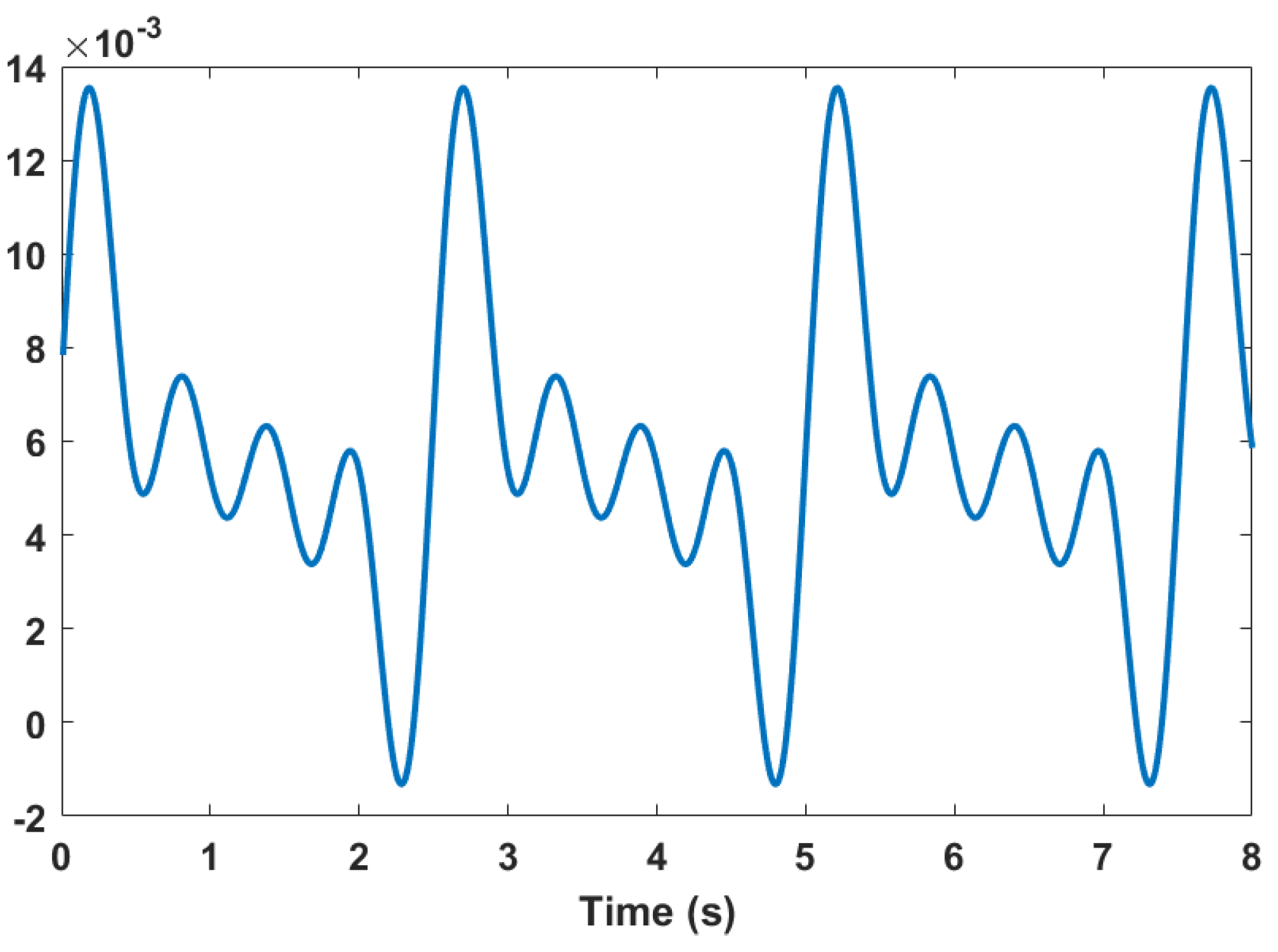
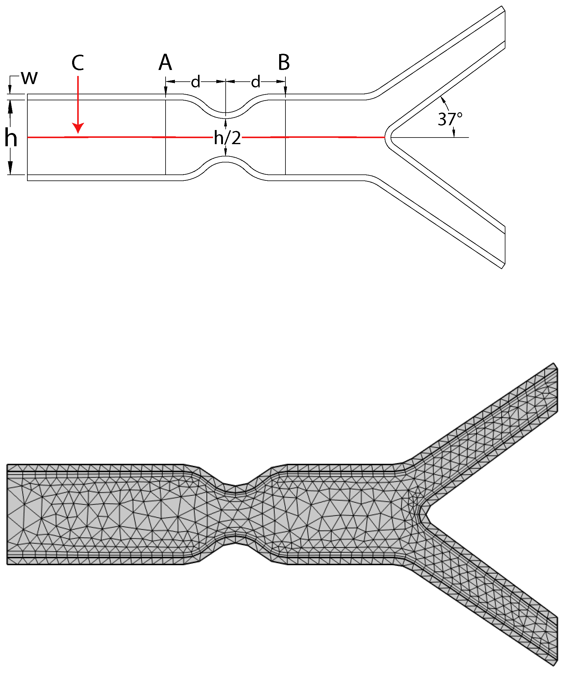
The boundary condition for the inlet velocity profile is considered to be waveform as shown in Figure 1, while the outlet pressure is set to zero. The problem’s geometry and coarse mesh are depicted in Figure 2.

$$u_{in}=\overline{u}+\overline{u}\sum _{n=1}^4[{\alpha }_{1}cos\left(n\omega t\right)+{\alpha }_{2}sin\left(n\omega t\right)]$$

(19)

The outlet velocity is at zero pressure. The boundary condition related to the solid domain is a fixed-point constraint at start and end, and other parts of the domain are free for movement due to flow. Pressure dictates the outflow boundary conditions. At the outflow, the pressure equalises to zero. In dimensionless form, the blood vessel wall contact criteria are as follows:

$${\displaystyle \frac{\partial d_s}{\partial t}}=u,E\sigma ·n=p\nabla u-pI.$$

(20)

The temperature boundary conditions are set in such a way that $\theta =1$ at the outer layer of the solid wall and no heat transfer at the inlet and outlet. Initially, velocity, displacement and temperature are set equal to zero.

As illustrated in Figure 2, a prototype geometric model is regarded. Stenosis and a bifurcation with a symmetrical arrangement are part of the computational domain. The walls are supposed to consist of isotropic and linear elastic materials characterized by Young’s modulus and Poisson ratio. The Lame coefficient $\lambda$, $\nu$ and shear modulus $\mu$ are therefore described. They conform to the following relationships:

$$\begin{array}{cc}\hfill \nu & ={\displaystyle \frac{1}{2}}·{\displaystyle \frac{\lambda }{(\mu +\lambda )}},\lambda ={\displaystyle \frac{E\nu }{(1+\mu )(1-2\nu )}},\hfill \end{array}$$

(21)

where $\nu =0.5$ represents the incompressible structure and $\nu <0.5$ represents the compressible structure; see [13]. Unless otherwise specified, we use Young’s modulus $E=1\times {10}^8$ Pa and Poisson ratio $\nu =0.49$, and viscosity is ${\nu }_f=3.3\times {10}^{-3}$${\mathrm{cm}}^2/\mathrm{s}$.

As illustrated in Figure 2, the diameter h is considered to be 1 cm and shrinks to $50\%$ at the region of stenosis. This implies that stenosis restricts the artery about $50\%$ of the time. The elastic wall’s width w is estimated to be $0.1$ cm. Further, ${37}^{\circ }$ is the inclination of the bifurcation artery. C is the central line along which pressure is recorded. A and B are chosen only to anticipate the behavior of the velocity profile prior to and following stenosis.

Additionally, the coarse mesh is shown in Figure 2. The geometry is converted to a tiny finite number of components using a triangular mesh. The coarse mesh consists of 1354 domain elements and 312 boundary elements.

Table 1. For $Gr=25$: Absolute error for the average Nusselt number at lower wall against the Grashof number against refinement level showing mesh independence for $E=1\times {10}^8$, $t=0.2$.

Level	Number of Elements	Avg. Nuss. Nr.	Abs. Error
0	1354	0.02769	-
1	5416	0.02770	0.000091
2	21,664	0.02771	0.000145
3	86,656	0.02770	0.000149
4	346,624	0.02770	0.000060
5	1,386,496	0.02770	0.000007

shows the absolute error of the average Nusselt number as a function of mesh refinement level and the number of elements.

3. Finite Element Discretization Using P2P1 Element Pair

In this formulation, quadratic (P2) elements are used to approximate the velocity components $(u,v)$, solid displacement $d_s$, and temperature field $\theta$, while linear (P1) elements are assigned to represent the pressure field p [14,15,16].

3.1. FEM Approximation for Fluid, Solid, and Temperature Fields

The unknown variables are approximated using basis functions.

Fluid velocity $(u,v)$ and mesh velocity $\left(w\right)$:

$$u_h=\sum _{i=1}^{N_u}{N}_i^2{U}_i,v_h=\sum _{i=1}^{N_u}{N}_i^2{V}_i$$

(22)

Fluid pressure p (using P1 elements):

$$p_h=\sum _{j=1}^{N_p}{M}_j^1{P}_j$$

(23)

Solid displacement $d_s$:

$$d_s=\sum _{k=1}^{N_d}{L}_k^2{D}_k$$

(24)

Temperature $\theta$:

$${\theta }_h=\sum _{m=1}^{N_{\theta }}{P}_m^2{T}_m$$

(25)

The terms $N_i^2,L_k^2,$ and $P_m^2$ represent quadratic basis functions associated with P2 elements, while $M_j^1$ corresponds to linear basis functions used in P1 elements. The variables $U_i,V_i,P_j,D_k,$ and $T_m$ denote the nodal values for velocity components, pressure, solid displacement, and temperature, respectively.

3.2. Weak Form Discretization

The weak form of the governing equations is formulated using appropriate function spaces for trial and test functions. For the fluid mechanics equations (Navier–Stokes), the velocity field $(u,v)$ is approximated in the Sobolev space ${\mathbf{V}}_u\subset H^1\left({\mathrm{\Omega }}_f\right)$, while the pressure field p belongs to the space $Q_p\subset L^2\left({\mathrm{\Omega }}_f\right)$. The corresponding test functions $\psi$ and q for velocity and pressure, respectively, are chosen from the same spaces. In the solid mechanics equations, the displacement field $d_s$ is defined in ${\mathbf{V}}_d\subset H^1\left({\mathrm{\Omega }}_s\right)$, with the test function $\phi$ also taken from ${\mathbf{V}}_d$. For heat transfer, the temperature field $\theta$ is approximated in $V_{\theta }\subset H^1\left(\mathrm{\Omega }\right)$, with test functions $\varphi$ selected from the same space. These function spaces ensure that trial and test functions are square-integrable and, where necessary, have square-integrable derivatives, satisfying the mathematical requirements for the Galerkin finite element method. The choice of the same function spaces for trial and test functions reflects the Galerkin framework and ensures the consistency of the weak formulation.

3.2.1. Fluid Equations (Navier–Stokes)

Momentum Conservation in X-direction:

$${\int }_{{\mathrm{\Omega }}_f}\left({\displaystyle \frac{\partial u}{\partial t}}\psi +(u-w){\displaystyle \frac{\partial u}{\partial x}}\psi +(v-w){\displaystyle \frac{\partial u}{\partial y}}\psi \right)d\mathrm{\Omega }-{\int }_{{\mathrm{\Omega }}_f}p\nabla ·\psi d\mathrm{\Omega }+{\int }_{{\mathrm{\Omega }}_f}{\displaystyle \frac{1}{Re}}\nabla u·\nabla \psi d\mathrm{\Omega }=0$$

(26)

Momentum Conservation in Y-direction:

$${\int }_{{\mathrm{\Omega }}_f}\left({\displaystyle \frac{\partial v}{\partial t}}\psi +(u-w){\displaystyle \frac{\partial v}{\partial x}}\psi +(v-w){\displaystyle \frac{\partial v}{\partial y}}\psi \right)d\mathrm{\Omega }-{\int }_{{\mathrm{\Omega }}_f}p\nabla ·\psi d\mathrm{\Omega }+{\int }_{{\mathrm{\Omega }}_f}{\displaystyle \frac{1}{Re}}\nabla v·\nabla \psi d\mathrm{\Omega }+{\int }_{{\mathrm{\Omega }}_f}{\displaystyle \frac{Gr}{R{e}^2}}\theta \psi d\mathrm{\Omega }=0$$

(27)

Continuity Equation (Incompressibility Constraint):

$${\int }_{{\mathrm{\Omega }}_f}q\nabla ·ud\mathrm{\Omega }=0$$

(28)

3.2.2. Solid Mechanics

$${\int }_{{\mathrm{\Omega }}_s}{\rho }_r{\displaystyle \frac{d^2{d}_s}{d{t}^2}}\phi d\mathrm{\Omega }+{\int }_{{\mathrm{\Omega }}_s}E\nabla \sigma ·\phi d\mathrm{\Omega }=0$$

(29)

3.2.3. Heat Transfer

$${\int }_{\mathrm{\Omega }}\left({\displaystyle \frac{\partial \theta }{\partial t}}\varphi +(u-w){\displaystyle \frac{\partial \theta }{\partial x}}\varphi +(v-w){\displaystyle \frac{\partial \theta }{\partial y}}\varphi \right)d\mathrm{\Omega }-{\int }_{\mathrm{\Omega }}\nabla \theta ·\nabla \varphi d\mathrm{\Omega }=0$$

(30)

3.3. Coupling Conditions

At the fluid–structure interface, we impose

$$U_f={\displaystyle \frac{\partial D_s}{\partial t}},{\sigma }_f·n={\sigma }_s·n$$

(31)

The global matrix is obtained from the monolithic system of equations following the discretization process using the finite element method (FEM):

$$\left[\begin{array}{ccccc}{M}_f& 0& C^T& 0& 0\\ 0& M_f& 0& C^T& {\displaystyle \frac{Gr}{R{e}^2}}{M}_T\\ C& 0& 0& 0& 0\\ 0& C& 0& 0& 0\\ 0& 0& 0& 0& M_T\end{array}\right]\left[\begin{array}{c}\dot{u}\\ \dot{v}\\ p\\ \dot{d}\\ \dot{\theta }\end{array}\right]+\left[\begin{array}{ccccc}{A}_f& 0& G^T& C_{fs}^T& 0\\ 0& A_f& 0& C_{fs}^T& 0\\ G& 0& 0& 0& 0\\ C_{fs}& C_{fs}& 0& K_s& 0\\ 0& 0& 0& 0& K_T\end{array}\right]\left[\begin{array}{c}u\\ v\\ p\\ d\\ \theta \end{array}\right]=\left[\begin{array}{c}{F}_x\\ F_y\\ 0\\ F_s\\ F_T\end{array}\right].$$

(32)

In this formulation, $M_f$ represents the fluid mass matrix, while $A_f$ corresponds to the fluid convection–diffusion matrix. The term G denotes the pressure gradient matrix, and C accounts for the coupling matrix used in Arbitrary Lagrangian–Eulerian (ALE) mesh movement. The interaction between the fluid and structure is captured by $C_{fs}$, the fluid–structure coupling matrix. Additionally, $K_s$ represents the solid stiffness matrix, whereas $K_T$ and $M_T$ correspond to the thermal diffusion matrix and thermal mass matrix, respectively. The coupling term for buoyancy effects in natural convection is given by $Gr{M}_T$, and the force contributions from the governing equations are denoted as $F_x,F_y,F_s,$ and $F_T$.

Coupling Effects of Temperature $\theta$: The temperature field $\theta$ plays a significant role in affecting fluid motion by introducing buoyancy-driven forces. This influence is captured through the Grashof number ($Gr$), which appears in the momentum equation and accounts for the interaction between thermal variations and fluid flow dynamics.

$${\int }_{{\mathrm{\Omega }}_f}{\displaystyle \frac{Gr}{R{e}^2}}\theta \psi d\mathrm{\Omega },$$

(33)

This term represents the effect of temperature variations on velocity due to buoyancy forces. The heat equation governing temperature evolution is

$$M_T\dot{\theta }+K_T\theta =F_T,$$

(34)

in this formulation, $M_T$ represents the thermal mass matrix, which governs transient heat conduction, while $K_T$ corresponds to the thermal conductivity matrix, responsible for controlling steady-state diffusion. The term $F_T$ denotes the external heat source or boundary heat flux. This approach is essential for accurately modeling fluid–structure interaction (FSI) with heat transfer and plays a crucial role in simulating arterial blood flow.

3.4. LBB (Ladyzhenskaya–Babuška–Brezzi) Condition for This Problem

In the context of our fluid–structure interaction (FSI) with the heat transfer problem, the Ladyzhenskaya–Babuška–Brezzi (LBB) condition plays a crucial role in maintaining numerical stability (for details, see [14,15]). It ensures that the velocity-pressure finite element discretization remains stable, preventing issues related to the incompressibility constraint $\nabla ·u=0$, which could otherwise lead to spurious pressure modes. Additionally, it helps avoid singular or ill-conditioned systems, ensuring the reliability and accuracy of the numerical solution.

3.4.1. Mathematical Formulation of the LBB Condition

The Ladyzhenskaya–Babuka–Brezzi (LBB) condition establishes the stability of the velocity-pressure pairing, $\left(U\right(u,v),p)$, velocity and pressure spaces, respectively; $V=H_0^1\left(\mathrm{\Omega }\right)$, $Q=L_2^0\left(\mathrm{\Omega }\right)$. It states that there exists a positive constant ${\beta }_1$, such that

$$\underset{U\in V}{sup}{\displaystyle \frac{{\int }_{\mathrm{\Omega }}(\nabla ·U)qd\mathrm{\Omega }}{{\parallel U\parallel }_{H^1}}}\ge {\beta }_1{\parallel q\parallel }_{L^2},\forall q\in Q.$$

(35)

Application of the LBB Condition in the FSI Problem: In the context of fluid–structure interaction (FSI) with heat transfer, the governing global system consists of multiple coupled equations. These include the Navier–Stokes equations, which describe the behavior of fluid velocity components $u,v$ along with the pressure field p, the incompressibility constraint $\nabla ·u=0$, which enforces mass conservation, the elasticity equations, which model the solid displacement d, and the heat transfer equation, which governs the temperature distribution $\theta$.

3.4.2. Proof of the LBB Condition

3.4.3. Step 1: Weak Formulation of Navier–Stokes

The weak form of the momentum equation is

$${\int }_{{\mathrm{\Omega }}_f}\rho \left({\displaystyle \frac{\partial U}{\partial t}}+U·\nabla U\right)Vd\mathrm{\Omega }-{\int }_{{\mathrm{\Omega }}_f}P(\nabla ·V)d\mathrm{\Omega }+{\int }_{{\mathrm{\Omega }}_f}\mu \nabla U:\nabla Vd\mathrm{\Omega }=0.$$

(36)

For the continuity equation,

$${\int }_{{\mathrm{\Omega }}_f}Q(\nabla ·U)d\mathrm{\Omega }=0.$$

(37)

3.4.4. Step 2: Stability Analysis

We define the bilinear form:

$$B(U,p)={\int }_{{\mathrm{\Omega }}_f}(p\nabla ·U)d\mathrm{\Omega }.$$

(38)

By integration by parts,

$$\underset{U\in V}{sup}{\displaystyle \frac{{\int }_{{\mathrm{\Omega }}_f}(\nabla ·U)pd\mathrm{\Omega }}{{\parallel U\parallel }_{H^1}}}\ge {\beta }_1{\parallel p\parallel }_{L^2},$$

(39)

this guarantees that the pressure is uniquely determined by the velocity field.

3.4.5. Step 3: Finite Element Discretization and LBB Condition

Using finite element spaces $V_h$ and $Q_h$, the discrete version of the LBB condition is

$$\underset{U_h\in V_h}{sup}{\displaystyle \frac{{\int }_{{\mathrm{\Omega }}_f}(\nabla ·U_h)P_{h}d\mathrm{\Omega }}{\parallel U_h{\parallel }_{H^1}}}\ge {{\beta }_1}_h{\parallel p_h\parallel }_{L^2},\forall p_h\in Q_h,$$

(40)

for stability, we require that ${{\beta }_1}_h>0$, which depends on the choice of elements.

4. Solution Algorithm

A resulting residual matrix through a monolithic system of equations is

$$\mathbf{R}\left(\mathbf{X}\right)=\left[\begin{array}{c}{M}_f\dot{U}+A_{f}U+G^{T}P+C_{fs}^{T}D-F_x\\ M_f\dot{V}+A_{f}V+G^{T}P+C_{fs}^{T}D+{\displaystyle \frac{Gr}{R{e}^2}}{M}_T\theta -F_y\\ GU+GV-0\\ M_s\ddot{D}+K_{s}D-C_{fs}(U,V)-F_s\\ M_T\dot{\theta }+K_T\theta -F_T\end{array}\right]=0.$$

(41)

In this formulation, $M_f$ represents the fluid mass matrix, while $A_f$ corresponds to the nonlinear convective term in the fluid equations. The pressure gradient matrix is denoted by G, and $C_{fs}$ accounts for the fluid–structure coupling within the system. The solid mass and stiffness matrices are given by $M_s$ and $K_s$, whereas $M_T$ and $K_T$ represent the thermal mass and thermal conductivity matrices, respectively. The term $Ri{M}_T$ captures the buoyancy effect coupling due to temperature variations. Finally, $F_x,F_y,F_s,$ and $F_T$ denote the external force components acting within the system.

4.1. Newton–Raphson Linearization for the Global Matrix $[u,v,p,d,\theta ]$

Since $A_{f}U$ is nonlinear (due to the convective term $u·\nabla u$), we solve the system using Newton–Raphson iterations.

4.1.1. Step 1: Linearization

We approximate the solution at iteration k as

$${\mathbf{X}}^{(k+1)}={\mathbf{X}}^{\left(k\right)}+\delta \mathbf{X},$$

(42)

expanding in a Taylor series and keeping only linear terms

$$\mathbf{R}\left({\mathbf{X}}^{(k+1)}\right)\approx \mathbf{R}\left({\mathbf{X}}^{\left(k\right)}\right)+J\left({\mathbf{X}}^{\left(k\right)}\right)\delta \mathbf{X}=0$$

(43)

where

• $\mathbf{R}\left(\mathbf{X}\right)$ is the residual vector,
• $J\left(\mathbf{X}\right)={\displaystyle \frac{\partial \mathbf{R}}{\partial \mathbf{X}}}$ is the Jacobian matrix,
• $\delta \mathbf{X}={[\delta u,\delta v,\delta p,\delta d,\delta \theta ]}^T$ is the correction vector.

4.1.2. Step 2: Solve for $\delta \mathbf{X}$

At each iteration, we solve

$$J\left({\mathbf{X}}^{\left(k\right)}\right)\delta \mathbf{X}=-\mathbf{R}\left({\mathbf{X}}^{\left(k\right)}\right)$$

(44)

4.2. Jacobian Matrix Formulation

The global Jacobian matrix J is

$$J=\left[\begin{array}{ccccc}{M}_f+A_f^{\prime }& 0& G^T& C_{fs}^T& 0\\ 0& M_f+A_f^{\prime }& 0& C_{fs}^T& {\displaystyle \frac{Gr}{R{e}^2}}{M}_T\\ G& G& 0& 0& 0\\ C_{fs}& C_{fs}& 0& K_s& 0\\ 0& 0& 0& 0& M_T+K_T\end{array}\right].$$

(45)

In this formulation, $A_f^{\prime }={\displaystyle \frac{\partial (u·\nabla u)}{\partial u}}$ represents the Jacobian matrix of the nonlinear convective term, capturing the sensitivity of the convective flow to velocity changes. The matrices G and $G^T$ are responsible for enforcing the incompressibility condition, ensuring that the velocity field remains divergence-free. The terms $C_{fs}$ and $C_{fs}^T$ establish the coupling between the fluid and solid domains, facilitating the interaction between the two. Additionally, $Ri{M}_T$ accounts for the coupling between temperature and velocity through the buoyancy effect, which influences fluid motion based on thermal variations.

4.3. Newton–Raphson Iterative Algorithm

The Newton–Raphson method proceeds as follows:

1.

Assemble and compute the residual vector $R\left(\mathbf{X}\right)$;

2.

Linearize using Newton–Raphson;

3.

Construct the Jacobian matrix $J\left(\mathbf{X}\right)$;

4.

Solve the linear system:

$$J\delta \mathbf{X}=-R\left(\mathbf{X}\right);$$

(46)

5.

Update the solution:

$${\mathbf{X}}^{(k+1)}={\mathbf{X}}^{\left(k\right)}+{\omega }^n\delta \mathbf{X};$$

(47)

6.

Repeat until convergence:

$$\left|\right|R\left(\mathbf{X}\right)\left|\right|<{ϵ}_1$$

(48)

where ${ϵ}_1$ is the tolerance criterion and ${\omega }^n\in (-1, 0]$ is the step length control; for details, see [17]. For a more detailed explanation, please refer to [18,19].

To Solve the Linearized Newton System

We deployed the PARDISO (Parallel Sparse Direct Solver), which is a high-performance solver optimized for solving large sparse linear systems of the form

$$Ax=b,$$

(49)

where A represents a large, sparse matrix, typically arising from the discretization of governing equations. The variable x denotes the solution vector, containing the unknowns to be determined, while b corresponds to the right-hand side vector, which incorporates external forces, boundary conditions, or source terms influencing the system.

It is particularly effective for symmetric, non-symmetric, and highly ill-conditioned sparse matrices, making it ideal for finite element analysis (FEA), fluid–structure interaction (FSI), and computational fluid dynamics (CFD) problems.

It employs a direct solver approach that utilizes LU, LDL^T, or Cholesky factorization, depending on the characteristics of the matrix A. The solver applies different factorization techniques based on the matrix type. For symmetric positive definite matrices, it implements Cholesky decomposition, which efficiently decomposes A into a product of a lower triangular matrix and its transpose, optimizing computational performance.

$$A=L{L}^T,$$

(50)

where L represents a lower triangular matrix, while $L^T$ denotes its transpose, which is an upper triangular matrix.

For general non-symmetric matrices,

$$A=LU,$$

(51)

where L represents a lower triangular matrix while U denotes an upper triangular matrix, both of which are obtained during the LU factorization process, enabling efficient numerical solution.

Symmetric Indefinite Matrices,

$$A=LD{L}^T,$$

(52)

where L denotes a lower triangular matrix and D represents a diagonal matrix. After completing the factorization, it computes x using forward and backward substitution.

1.

Forward substitution: We solve for y.

$$Ly=b$$

(53)

2.

Backward substitution: We solve for x.

$$Ux=y$$

(54)

This ensures an exact solution within machine precision, making direct solvers more robust than iterative methods. PARDISO is widely used in COMSOL [20] and FEM solvers due to its parallelization and numerical stability.

5. Results and Discussion

The following part shows the velocity profile, energy transmission, wall shear stress, and elastic wall displacement for bifurcation stenosis arteries over various time intervals. In the current analysis, the moving mesh-finite element method is used for resolution of non-linear mixed partial differential equations in dimensionless form. Prandtl is assumed to be $Pr=30$ in this study. We studied the difference in velocity profile, temperature distribution comportability, and isothermal contours for various time intervals such as $t=0.2$ s, $0.4$ s, $0.6$ s, and $0.8$ s, respectively.

Velocity profile variance results were evaluated for results of the wave shape inlet boundary at different intervals described above. The speed corresponds closely to the interval, as with time span and good difference before and after the plaque, waveform entry increases. There is also a noticeable effect on the elastic wall of the bottom state of the entry wave form and consequently the speed profile changes along the wall.

The health of the cardiovascular system may be compromised due to the presence of flow recirculation from a medical point of view. The patient indeed has atherosclerosis because in this condition, the circulation of blood flows very slowly. From now on, we should carry out further studies in this area to strengthen our understanding of the arterial system and cure for the illness.

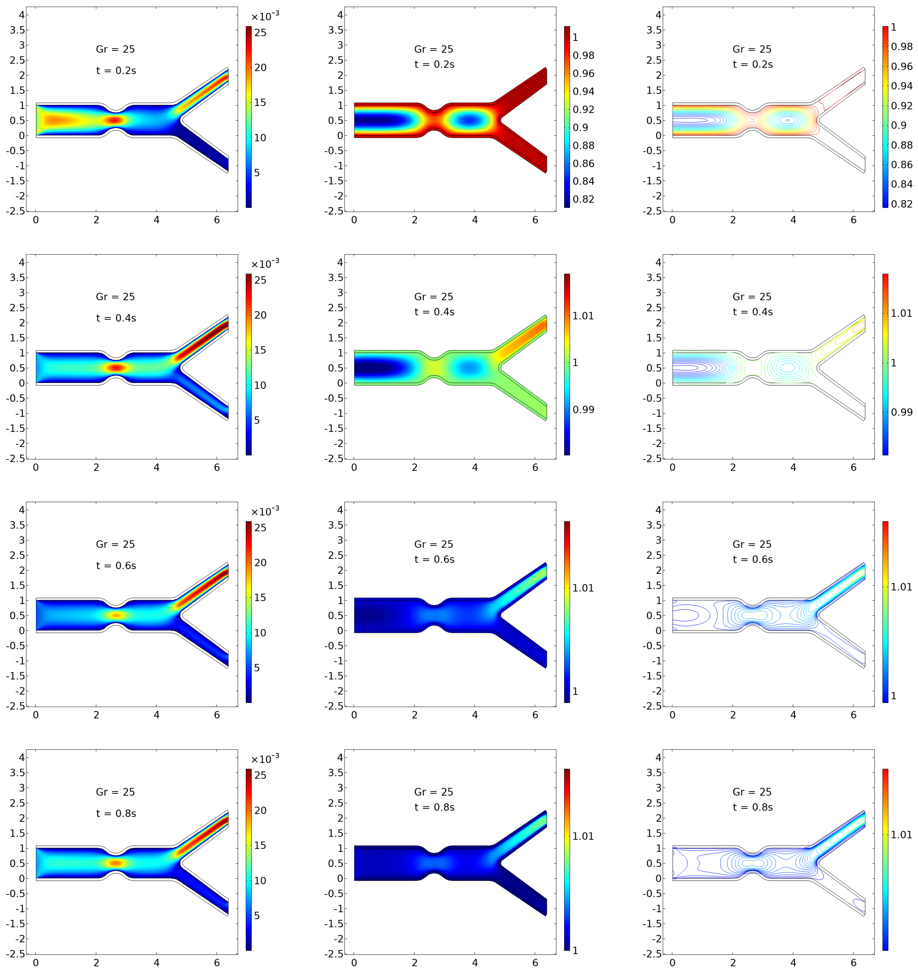
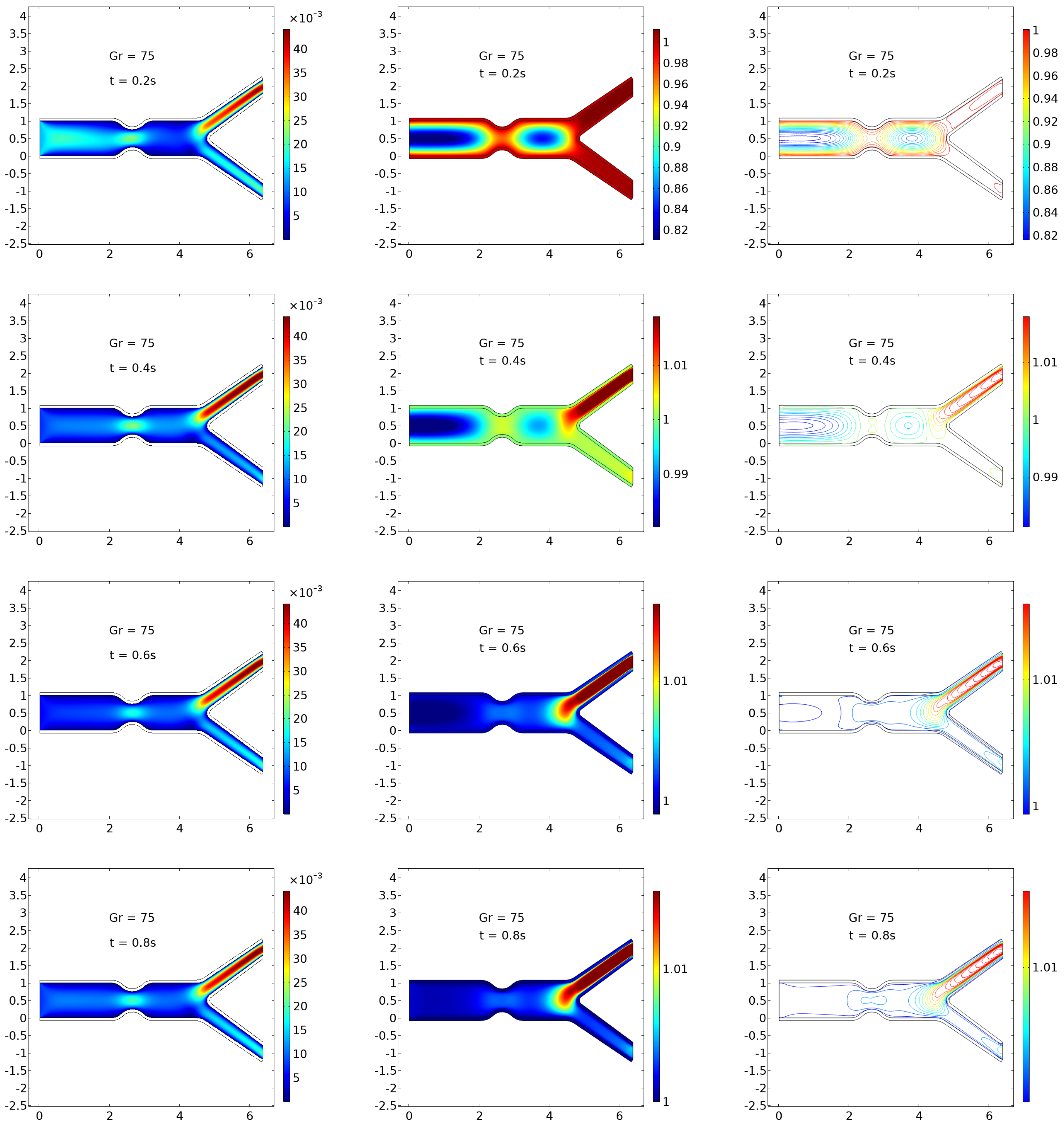
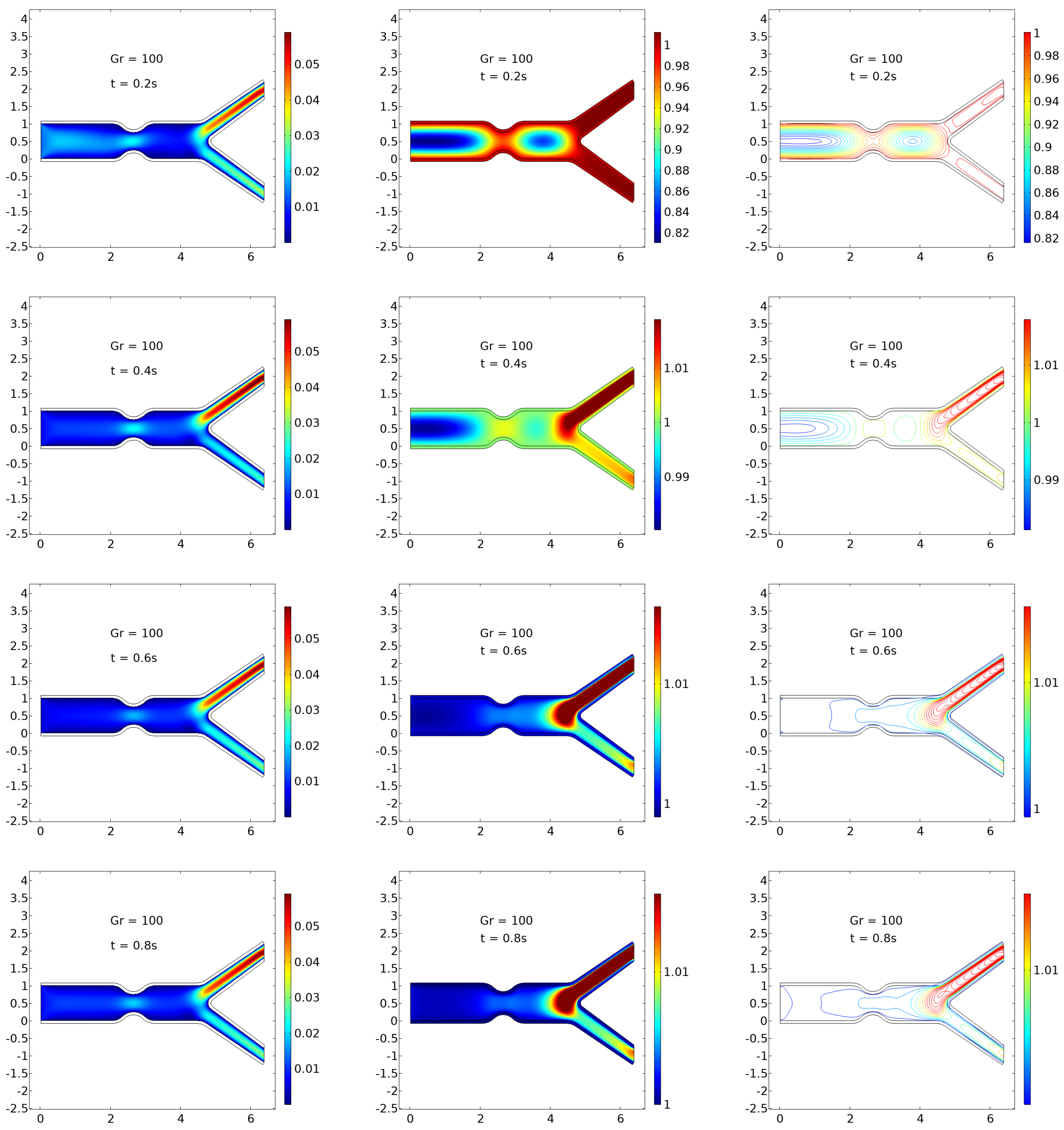
Figure 3, Figure 4, Figure 5 and Figure 6 provide a progressive visualization of the hemodynamic and thermal behaviors in a bifurcated stenosed artery model under increasing Grashof numbers ($Gr=25,50,75,100$) and at four distinct time intervals ($t=0.2$ s, $0.4$ s, $0.6$ s, $0.8$ s). Each figure presents three facets of the system’s behavior: velocity surface plots (left), temperature surface plots (center), and isothermal contour plots (right), capturing the intricate dynamics between blood flow, heat transport, and elastic arterial walls.

At $Gr=25$ (Figure 3), the flow remains mostly laminar with mild recirculation near the bifurcation and post-stenotic regions. The velocity peaks sharply near the constricted zone, with smoother downstream profiles as time progresses. The temperature distribution remains strongly localized near the arterial walls, and isotherms maintain a symmetric, stratified pattern. This behavior indicates dominance of conduction over convection, suitable for baseline physiological states.

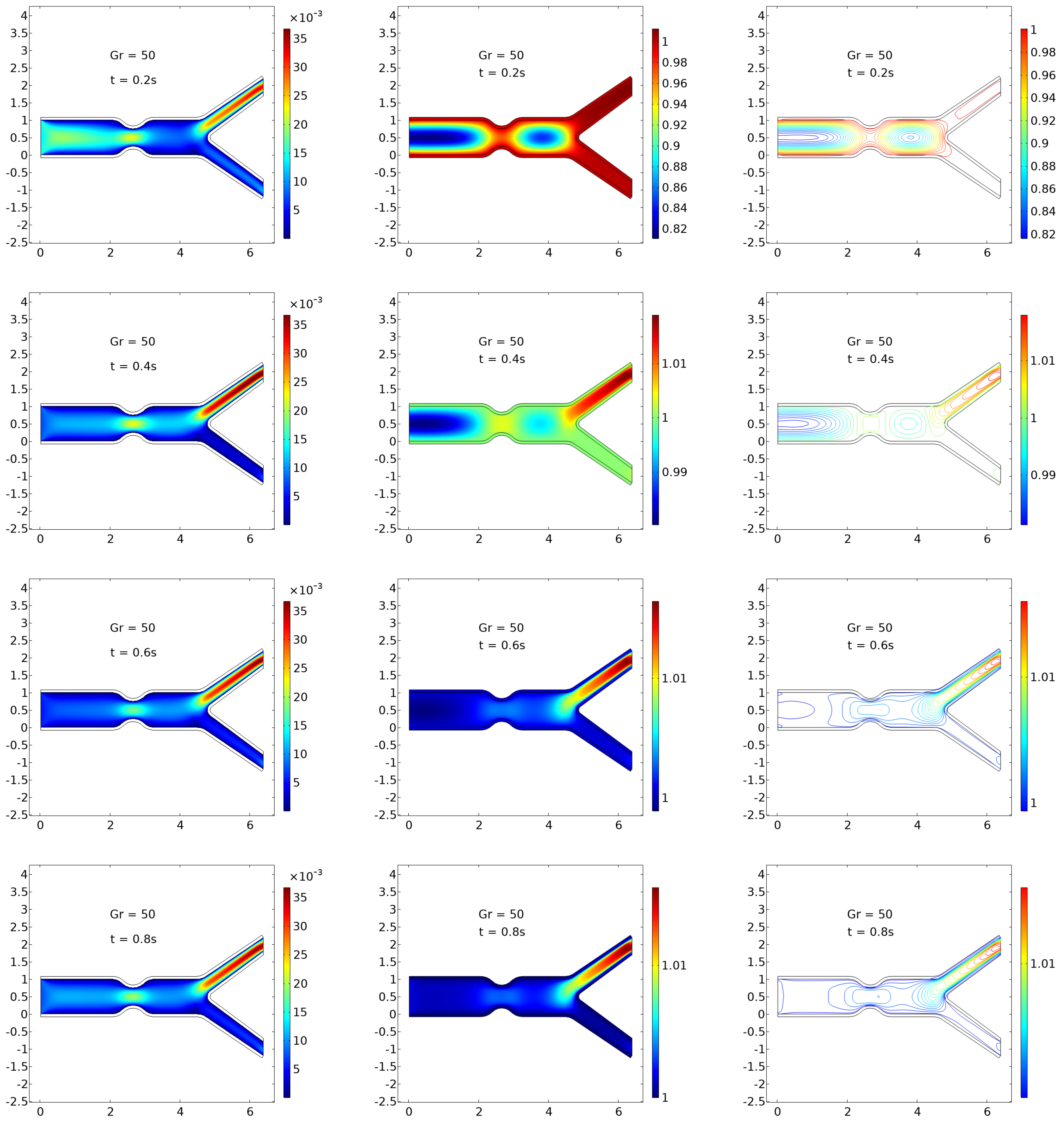
In Figure 4 ($Gr=50$), the onset of buoyancy effects becomes more pronounced. Flow profiles show increased disturbances and early vortex formation near bifurcation regions. Temperature surfaces exhibit greater penetration into the core fluid domain, and isotherms begin to lose symmetry, suggesting the role of natural convection in shaping the thermal field. These results indicate a transitional flow regime, where the coupling between thermal gradients and fluid momentum becomes significant.

Figure 5 ($Gr=75$) reveals further intensification of these effects. Recirculation zones become evident with stronger flow separation at bifurcations. Temperature fields show high gradients extending away from the walls, and thermal hotspots develop in the upper daughter artery. The isothermal contours exhibit substantial distortion, confirming nonlinear thermal transport and a shift toward mixed convection.

At the highest simulated Grashof number, $Gr=100$ (Figure 6), the system exhibits fully developed natural convection effects. The velocity fields are chaotic, with evident transient eddies and complex wall interactions. Thermal energy spreads into central flow zones, and localized heating becomes dominant. The isothermal plots reveal significant boundary layer detachment and contour fragmentation, highlighting the dominance of buoyancy-induced transport. These effects mirror thermally unstable or pathologically inflamed vascular environments.

Table 2. Average Nusselt number at lower wall against the Grashof number.

	$\mathit{E}=1\times {10}^{10}$				$\mathit{E}=1\times {10}^8$
Gr	t = 0.2	t = 0.4	t = 0.6	t = 0.8	t = 0.2	t = 0.4	t = 0.6	t = 0.8
25	0.15385	0.01311	0.00546	0.00683	0.02779	0.00234	0.0009	0.00118
50	0.15654	0.01077	0.00665	0.00869	0.02827	0.00192	0.00118	0.00153
75	0.17266	0.01934	0.01584	0.01851	0.03117	0.00348	0.00287	0.00333
100	0.17824	0.03277	0.03414	0.03682	0.03216	0.00596	0.00624	0.00670

and

Table 3. Average Nusselt number at upper wall against the Grashof number.

	$\mathit{E}=1\times {10}^{10}$				$\mathit{E}=1\times {10}^8$
Gr	t = 0.2	t = 0.4	t = 0.6	t = 0.8	t = 0.2	t = 0.4	t = 0.6	t = 0.8
25	0.16459	0.03654	0.02604	0.02648	0.02971	0.00664	0.00475	0.00479
50	0.18071	0.05881	0.04763	0.04797	0.03260	0.01073	0.00871	0.00874
75	0.21143	0.09206	0.07729	0.07758	0.03815	0.01683	0.01416	0.01417
100	0.23366	0.13149	0.11756	0.11643	0.04223	0.02407	0.02155	0.02131

depict the behavior of the average Nusselt number against two different values of elastic modulus. A significant difference can be noticed in the value of the average Nusselt number, and this clearly indicates that we cannot ignore the elastic effect of arteries. The value of the average Nusselt number increases with an increase in $Gr$.

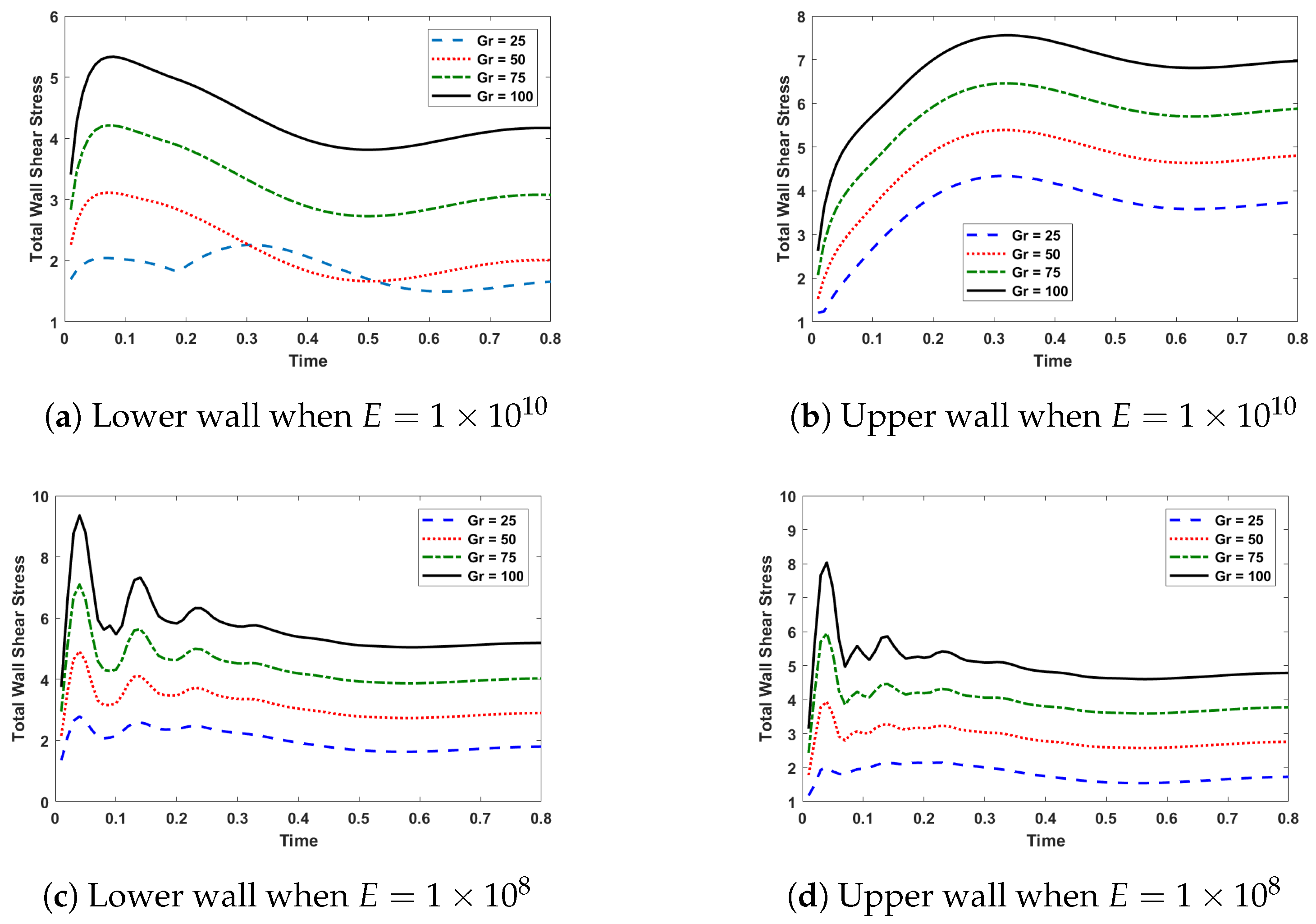
Wall shear stress (WSS) is an important factor to observe as it helps to reduce recirculation area in a stenosed artery. In Figure 7, WSS behavior can be observed against time for different value of $Gr$. In the case of the upper wall, the value of maximum total WSS increases compared to the lower wall. The magnitude of WSS increases with increase in $Gr$. Consequently, the chance of atherosclerosis is reduced.

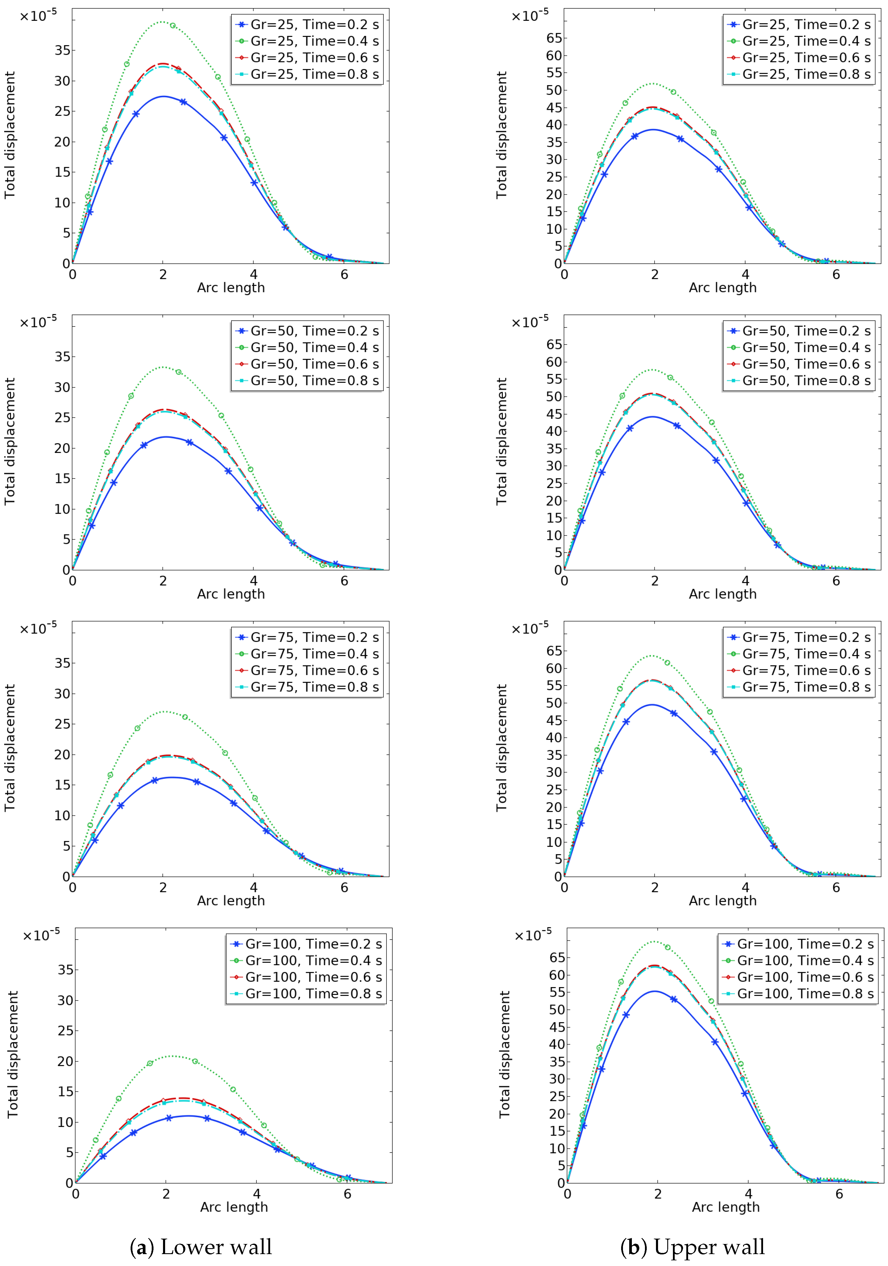
In Figure 8, wall deformation behavior is shown. Large deformation is spotted at the stenoses position. The deformation gradually increases with time. As the value of $Gr$ increases, the displacement or deformation decreases.

6. Conclusions

A two-dimensional time-dependent thermo-fluid model is developed and numerically evaluated for an elastic bifurcation stenosis artery. The implementation of a detailed model for energy transport inside fluid–structure interaction constitutes a novel feature of the work. The current model can therefore estimate the effect of the flow rate and the pressure on the temperature, as well as that of the displacement of elastic walls. The effect on heat transfer of the structural properties of the vessel wall and different other properties is studied. Due to the fact that the transport velocity for temperature is the fluid velocity, the fluid temperature is also influenced by a parameter that determines velocity.

Fluid and solid (elasticity) governing equations are discretized by imposing a strong formulation of coupled products utilising the Arbitrary Lagrangian–Eulerian method. The resulting system is resolved further using the Newton Raphson procedure. The results are graphically and tabularly displayed. Our results arewidely translated, which means the following:

• It is observed that temperature dominantly affacts blood velocity amidst elastic walls.
• The inlet velocity profile plays a vital role in the displacement of the wall for small time intervals.
• The elastic behavior of walls decreases the average Nusselt number.
• The temperature plots are in good agreement with the considered model.
• Wall shear stress (WSS) and displacement are prominently analyzed during prescribed time intervals.

Future research based on patient-specific data will certainly extend the explanations in detail. Hence, we believe that future investigations are necessary to ratify the kinds of conclusions that can be drawn from this study and incorporating the biomedical data.

The observed progression across Figure 3, Figure 4, Figure 5 and Figure 6 underscores the critical influence of thermal buoyancy on hemodynamics and arterial heat transfer. Under baseline conditions ($Gr=25$), the behavior aligns with physiological expectations, where blood flow and heat transfer remain laminar and wall-confined. As $Gr$ increases, the flow becomes more disturbed, and natural convection augments thermal transport, particularly under conditions that simulate localized inflammation or external heating (e.g., during fever or thermal therapy).

Regions of recirculation and flow separation, observed especially in Figure 5 and Figure 6, are clinically significant as they correspond to zones of low wall shear stress—key contributors to the development of atherosclerotic plaques. Moreover, elevated thermal gradients near bifurcations can alter endothelial cell responses and may influence the efficacy of temperature-based treatments such as hyperthermia or laser ablation.

The combined velocity and thermal data provide essential insight into the interaction between fluid–structure dynamics and bioheat transfer, supporting the development of patient-specific models for diagnosis and therapeutic planning. The results emphasize the need for careful consideration of buoyancy and pulsatility in computational modeling of cardiovascular flows, especially in diseased or surgically altered geometries.

References

- Razzaq, M.; Anwar, M.A.; Iqbal, K.; Haq, I.; Gurris, M. A Phenomenological Fluid–Structure Interaction Study of Plaque Rupture in Stenosed Bifurcated Elastic Arteries. Mathematics 2025, 13, 621. [Google Scholar] [CrossRef]
- Qiao, Y.; Luo, K.; Fan, J. Heat transfer mechanism in idealized healthy and diseased aortas using fluid–structure interaction method. Biomech. Model. Mechanobiol. 2023, 22, 1953–1964. [Google Scholar] [CrossRef] [PubMed]
- Luan, J.; Qiao, Y.; Mao, L.; Fan, J.; Zhu, T.; Luo, K. The role of aorta distal to stent in the occurrence of distal stent graft-induced new entry tear: A computational fluid dynamics and morphological study. Comput. Biol. Med. 2023, 166, 107554. [Google Scholar] [CrossRef] [PubMed]
- Liu, J.; Yang, W.; Lan, I.S.; Marsden, A.L. Fluid-structure interaction modeling of blood flow in the pulmonary arteries using the unified continuum and variational multiscale formulation. Mech. Res. Commun. 2020, 107, 103556–103563. [Google Scholar] [CrossRef] [PubMed]
- Foong, L.K.; Shirani, N.; Toghraie, D.; Zarringhalam, M.; Afrand, M. Numerical simulation of blood flow inside an artery under applying constant heat flux using Newtonian and non-Newtonian approaches for biomedical engineering. Comput. Methods Programs Biomed. 2020, 190, 105375–105381. [Google Scholar] [CrossRef] [PubMed]
- Chakravarty, S.; Sen, S. Dynamic response of heat and mass transfer in blood flow through stenosed bifurcated arteries. Korea-Aust. Rheol. J. 2005, 17, 47–62. [Google Scholar]
- Ley, O.; Kim, T. Calculation of arterial wall temperature in atherosclerotic arteries: Effect of pulsatile flow, arterial geometry, and plaque structure. BioMed. Eng. Online 2007, 6, 8. [Google Scholar] [CrossRef] [PubMed]
- Wang, C.Y. Heat Transfer to Blood Flow in a Small Tube. J. Biomech. Eng. 2008, 130, 024501-1–024501-3. [Google Scholar] [CrossRef] [PubMed]
- Jamali, M.S.A.; Ismail, Z. Simulation of Heat Transfer on Blood Flow through a Stenosed Bifurcated Artery. J. Adv. Res. Fluid Mech. Therm. Sci. 2019, 60, 310–323. [Google Scholar]
- Zhang, B.; Gu, J.; Qian, M.; Niu, L.; Zhou, H.; Ghista, D. Correlation between quantitative analysis of wall shear stress and intima-media thickness in atherosclerosis development in carotid arteries. Biomed. Eng. Online 2017, 16, 137. [Google Scholar] [CrossRef] [PubMed]
- Chato, D. Heat transfer to blood vessels. J. Biomech. Eng. 1980, 102, 110–118. [Google Scholar] [CrossRef] [PubMed]
- Zhang, X.; Zheng, L.; Wang, E.; Shu, C. Numerical investigations of temperature and hemodynamics in carotid arteries with and without atherosclerotic plaque during open surgery. J. Therm. Biol. 2020, 91, 622–632. [Google Scholar] [CrossRef] [PubMed]
- Razzaq, M.; Turek, S.; Hron, J.; Acker, J.F.; Weichert, F.; Wagner, M.; Grunwald, I.Q.; Roth, C.; Romeike, B.F. Numerical Simulation of fluid–structure Interaction with Application to Aneurysm Hemodynamics; Technical University, Fakultat fur Mathematik: Berlin, Germany, 2009. [Google Scholar]
- Brezzi, F. On the existence, uniqueness, and approximation of saddle-point problems arising from Lagrangian multipliers. Rev. Française d’Automatique Informatique Rech. Opérationnelle 1974, R.2, 129–151. [Google Scholar] [CrossRef]
- Brezzi, F.; Fortin, M. Mixed and Hybrid Finite Element Methods; Springer: Berlin/Heidelberg, Germany, 1991. [Google Scholar]
- Donea, J.; Huerta, A. Finite Element Methods for Flow Problems; Wiley: Hoboken, NJ, USA, 2003; ISBN 978-0-471-49666-3. [Google Scholar]
- Turek, S.; Hron, J.; Razzaq, M.; Wobker, H.; Schäfer, M. Numerical benchmarking of fluid–structure interaction: A comparison of different discretization and solution approaches. In fluid–structure Interaction II: Modelling, Simulation, Optimisation; Bungartz, H.-J., Mehl, M., Schäfer, M., Eds.; Volume 73 of Lecture Notes in Computational Science and Engineering; Springer: Berlin/Heidelberg, Germany, 2010; pp. 413–424. [Google Scholar]
- Hron, J.; Turek, S. A Monolithic FEM/Multigrid Solver for ALE Formulation of fluid–structure Interaction with Application in Biomechanics; Lecture Notes in Computational Science and Engineering; Springer: Berlin/Heidelberg, Germany, 2006; Volume 53, pp. 146–170. [Google Scholar]
- Turek, S.; Rivkind, L.; Hron, J.; Glowinski, R. Numerical study of a modified time-steping θ-scheme for incompressible flow simulations. J. Sci. Comput. 2006, 28, 533–547. [Google Scholar] [CrossRef]
- COMSOL Multiphysics®; v. 6.3. COMSOL AB: Stockholm, Sweden. Available online: www.comsol.com (accessed on 10 January 2025).