First-Hitting Problems for Jump-Diffusion Processes with State-Dependent Uniform Jumps

Abstract

Let $\left\{X\right(t),t\ge 0\}$ be a one-dimensional jump-diffusion process whose continuous part is either a Wiener, Ornstein–Uhlenbeck, or generalized Bessel process. The process starts at $X\left(0\right)=x\in [-d,d]$. Let $\tau \left(x\right)$ be the first time that $X\left(t\right)=0$ or $\left|X\right(t\left)\right|=d$. The jumps follow a uniform distribution on the interval $(-2x,0)$ when x is positive and on the interval $(0,-2x)$ when x is negative. We are interested in the moment-generating function of $\tau \left(x\right)$, its mean, and the probability that $X\left[\tau \right(x\left)\right]=0$. We must solve integro-differential equations, subject to the appropriate boundary conditions. Analytical and numerical results are presented.

1. Introduction

Let $\{X_0\left(t\right),t\ge 0\}$ be a one-dimensional diffusion process defined by the stochastic differential Equation (see [1])

$$\mathrm{d}{X}_0\left(t\right)=f_0\left[X_0\left(t\right)\right]\mathrm{d}t+{\left\{v_0\left[X_0\left(t\right)\right]\right\}}^{1/2}\mathrm{d}{B}_0\left(t\right),$$

(1)

where $\{B_0\left(t\right),t\ge 0\}$ is a standard Brownian motion. Assume that $X_0\left(0\right)=x\in [a,b]$ and define the first-hitting time (or first-passage time)

$${\tau }_0\left(x\right)=inf\{t\ge 0:X_0\left(t\right)\notin (a,b)\mid X_0\left(0\right)=x\in [a,b]\},$$

(2)

where we assume that the boundaries at $x=a$ and $x=b$ are attainable in finite time. The moment-generating function

$$M_0(x;s):=E\left[e^{-s{\tau }_0\left(x\right)}\right],$$

(3)

where $s>0$, of the random variable ${\tau }_0\left(x\right)$ satisfies the Kolmogorov backward equation

$${\displaystyle \frac{1}{2}}{v}_0\left(x\right)M_0^{″}(x;s)+f_0\left(x\right)M_0^{\prime }(x;s)=s{M}_0(x;s)$$

(4)

for $a<x<b$; see, for example, Cox and Miller [2]. Moreover the boundary conditions are $M_0(a;s)=M_0(b;s)=1$. Similarly, the function $m_0\left(x\right):=E\left[{\tau }_0\left(x\right)\right]$ (if it exists) satisfies the ordinary differential Equation (ODE)

$${\displaystyle \frac{1}{2}}{v}_0\left(x\right)m_0^{″}\left(x\right)+f_0\left(x\right)m_0^{\prime }\left(x\right)=-1,$$

(5)

subject to $m_0\left(a\right)=m_0\left(b\right)=0$. Finally, the probability $p_0\left(x\right):=P[X_0\left({\tau }_0\left(x\right)\right)=a]$ is a solution of the ODE

$${\displaystyle \frac{1}{2}}{v}_0\left(x\right)p_0^{″}\left(x\right)+f_0\left(x\right)p_0^{\prime }\left(x\right)=0,$$

(6)

and is such that $p_0\left(a\right)=1$ and $p_0\left(b\right)=0$. First-hitting problems have applications in many fields, notably biology and financial mathematics.

In this paper, we consider the stochastic process $\left\{X\right(t),t\ge 0\}$ defined by

$$X\left(t\right)=X\left(0\right)+{\int }_0^{t}f\left[X\left(s\right)\right]\mathrm{d}s+\sigma B\left(t\right)+\sum _{i=0}^{N\left(t\right)}{Y}_i,$$

(7)

where $f(·)$ is a real function such that $f(-x)=-f\left(x\right)$, $\sigma >0$, $\left\{B\right(t),t\ge 0\}$ is a standard Brownian motion process, $\left\{N\right(t),t\ge 0\}$ is a Poisson process with rate $\lambda$ (which is independent of $\left\{B\right(t),t\ge 0\}$), and $Y_1,Y_2,\dots$ are independent and identically distributed random variables. Moreover, we assume that f is such that $\left\{X\right(t),t\ge 0\}$ is a jump-diffusion process.

We define the first-hitting time

$$\tau \left(x\right)=inf\{t\ge 0:X(t)=0\mathrm{or}|X\left(t\right)|=d\mid X(0)=x\in [-d,d\left]\right\}$$

(8)

and we let $M(x;\alpha ):=E\left[e^{-\alpha \tau \left(x\right)}\right],$ where $\alpha >0$. It can be shown (see [3]) that the function $M(x;\alpha )$ satisfies the integro-differential Equation (IDE) (writing $M(x;\alpha )$ as $M\left(x\right)$)

$${\displaystyle \frac{1}{2}}{\sigma }^2{M}^{″}\left(x\right)+f\left(x\right)M^{\prime }\left(x\right)+\lambda \left\{{\int }_{-\infty }^{\infty }M(x+y)f_Y\left(y\right)\mathrm{d}y-M\left(x\right)\right\}=\alpha M\left(x\right),$$

(9)

where Y is distributed as the $Y_i$’s. The boundary conditions are $M\left(0\right)=M(\pm d)=1$.

Suppose that Y has a uniform distribution on the interval $(-2x,0)$ if $x>0$ and a uniform distribution on the interval $(0,-2x)$ if $x<0$. Then, by symmetry, we can write that $M(-x)=M\left(x\right)$, so that we can consider the process in the interval $[0,d]$ alone. Moreover, for $x>0$,

$$\begin{array}{ccc}\hfill {\int }_{-\infty }^{\infty }M(x+y)f_Y\left(y\right)\mathrm{d}y& =& {\displaystyle \frac{1}{2x}}{\int }_{-2x}^{0}M(x+y)\mathrm{d}y={\displaystyle \frac{1}{2x}}{\int }_{-x}^{x}M\left(z\right)\mathrm{d}z\hfill \\ & \stackrel{\mathrm{sym}.}{=}& {\displaystyle \frac{1}{x}}{\int }_0^{x}M\left(z\right)\mathrm{d}z.\hfill \end{array}$$

(10)

Hence, Equation (9) becomes

$${\displaystyle \frac{1}{2}}{\sigma }^2{M}^{″}\left(x\right)+f\left(x\right)M^{\prime }\left(x\right)+\lambda \left\{{\displaystyle \frac{1}{x}}{\int }_0^{x}M\left(z\right)\mathrm{d}z-M\left(x\right)\right\}=\alpha M\left(x\right)$$

(11)

for $0<x<d$.

Next, let $m\left(x\right):=E\left[\tau \right(x\left)\right]$ and $p\left(x\right):=P\left[X\right(\tau \left(x\right))=0]$. To obtain these functions, we need to solve the following equations:

$${\displaystyle \frac{1}{2}}{\sigma }^2{m}^{″}\left(x\right)+f\left(x\right)m^{\prime }\left(x\right)+\lambda \left\{{\displaystyle \frac{1}{x}}{\int }_0^{x}m\left(z\right)\mathrm{d}z-m\left(x\right)\right\}=-1,$$

(12)

subject to the boundary conditions $m\left(0\right)=m\left(d\right)=0$, and

$${\displaystyle \frac{1}{2}}{\sigma }^2{p}^{″}\left(x\right)+f\left(x\right)p^{\prime }\left(x\right)+\lambda \left\{{\displaystyle \frac{1}{x}}{\int }_0^{x}p\left(z\right)\mathrm{d}z-p\left(x\right)\right\}=0,$$

(13)

subject to $p\left(0\right)=1$ and $p\left(d\right)=0$.

A possible application of the problem studied in this paper is as follows: Suppose that $X\left(t\right)$ represents the position of an object (an aircraft, for example) at time t. The objective is to make the object in question follow a trajectory that corresponds to $x=0$. To do this, we correct the trajectory according to a Poisson process, trying to bring the object back to the origin with thrusts that follow a uniform distribution whose mean is $-x$, with x being the current position of the object. Note that, by continuity, the probability of a jump from x to 0 is equal to 0. Moreover, because the jumps are instantaneous, if the process jumps from a positive to a negative value (or vice versa), it is assumed that it did not hit the origin.

We will consider the following particular cases for the function $f\left(x\right)$:

• $f\left(x\right)\equiv 0$, so that $\left\{X\right(t),t\ge 0\}$ is a Wiener process with zero drift and with jumps.
• $f\left(x\right)=-\beta x$, where $\beta >0$, so that $\left\{X\right(t),t\ge 0\}$ is an Ornstein–Uhlenbeck process with jumps.
• ${\displaystyle f\left(x\right)=\frac{\gamma -1}{2x}}$, where $\gamma \in [0,2)$, so that $\left\{X\right(t),t\ge 0\}$ is a (generalized) Bessel process with jumps. The condition $\gamma \in [0,2)$ implies that the process can attain the origin; see [4].

Remark 1. 

(i) We used the expression generalized Bessel process, because a Bessel process is non-negative by definition. Therefore, if it reaches the origin, we assume that there is a reflecting (or an absorbing) boundary at $x=0$. However, a diffusion process that satisfies the stochastic differential equation

$$\mathrm{d}{X}_0\left(t\right)={\displaystyle \frac{\gamma -1}{2X_0\left(t\right)}}\mathrm{d}t+\mathrm{d}{B}_0\left(t\right)$$

(14)

can be considered for negative values when $\gamma \in [0,2)$. In particular, if $\gamma =1$, then $\{X_0\left(t\right),t\ge 0\}$ is a standard Brownian motion, which is a Gaussian process.

• (ii) The Wiener process, or Brownian motion, is the basic and most important diffusion process. The Ornstein–Uhlenbeck process is also very important for the applications. It was proposed by Uhlenbeck and Ornstein in [5] as a model for the velocity of a particle that is undergoing Brownian motion. The Bessel process was studied extensively in the book by Revuz and Yor [6]. These three diffusion processes are treated in most textbooks on stochastic processes, for instance, in the works of Karlin and Taylor [4] and Lefebvre [7].

Obtaining exact and explicit solutions to boundary value problems for integro-differential equations is a difficult task. The first author has written a number of papers on such problems; see, in particular, refs. [8,9]. He also considered optimal control problems known as homing problems for these processes.

A very important application of jump-diffusion processes is in financial mathematics; in his seminal paper, Merton [10] used these processes to model the behaviour of stock prices. Other papers on jump-diffusion processes include the following: Abundo [11,12], Cai [13], Peng and Liu [14], Yin et al. [15], Zhou and Wu [16], and Ai et al. [17].

In [18], Abundo computed the first-passage area of one-dimensional jump-diffusion processes. Lefebvre [19] also studied a first-passage-place problem for a one-dimensional jump-diffusion process and its integral.

Jump-diffusion processes are related to diffusion processes with stochastic resetting, but they are fundamentally different. These processes were first studied by Evans and Majumdar [20]; see also Abundo [21] and the references therein. In the case of a diffusion process with resetting times, according to a Poisson process, at random times that follow an exponential distribution, the process is reset instantaneously to a fixed value $x_R$ and then evolves from this position in accordance with the stochastic differential equation that defines the diffusion process. In contrast, when a jump occurs in a jump-diffusion process, the new position of the process is completely random and (when the jump size distribution is a continuous random variable) can never be the same.

In Section 2, we will obtain exact analytical expressions for the probability $p\left(x\right)$. We will first transform the IDE in Equation (13) into a third-order linear ODE. After solving this ODE, subject to two boundary conditions, we will determine the third constant which is such that the solution to the ODE also satisfies the corresponding IDE.

Next, in Section 3, numerical solutions for the mean $m\left(x\right)$ and the moment-generating function $M(x;\alpha )$ will be presented. We will see the effect of the jumps on the solutions by comparing these functions with the corresponding ones when there are no jumps (that is, when $\lambda =0$). Finally, we will end with a few remarks in Section 4.

2. Ordinary Differential Equations

Differentiating both sides of the IDE in Equation (11), we obtain (from Leibniz’s integral rule) that

$${\displaystyle \frac{1}{2}}{\sigma }^2{M}^{‴}\left(x\right)+f\left(x\right)M^{″}\left(x\right)+[f^{\prime }\left(x\right)-\lambda -\alpha ]M^{\prime }\left(x\right)+\lambda \left\{-{\displaystyle \frac{1}{x^2}}{\int }_0^{x}M\left(z\right)\mathrm{d}z+{\displaystyle \frac{1}{x}}M\left(x\right)\right\}=0.$$

(15)

Moreover, from Equation (11),

$${\displaystyle \frac{\lambda }{x}}{\int }_0^{x}M\left(z\right)\mathrm{d}z=-{\displaystyle \frac{1}{2}}{\sigma }^2{M}^{″}\left(x\right)-f\left(x\right)M^{\prime }\left(x\right)+(\lambda +\alpha )M\left(x\right).$$

(16)

Hence, we can state the following proposition.

Proposition 1. 

The moment-generating function $M\left(x\right)$ (= $M(x;\alpha )$) satisfies, for $\lambda >0$, the third-order linear ODE

$${\displaystyle \frac{1}{2}}{\sigma }^{2}x{M}^{‴}\left(x\right)+\left[xf\left(x\right)+{\displaystyle \frac{{\sigma }^2}{2}}\right]M^{″}\left(x\right)+\left\{x[f^{\prime }\left(x\right)-\lambda -\alpha ]+f\left(x\right)\right\}{M}^{\prime }\left(x\right)=\alpha M\left(x\right)$$

(17)

for $x\in (0,d)$. Moreover, we have the boundary conditions $M\left(0\right)=M\left(d\right)=1$.

Corollary 1. 

The mean $m\left(x\right)$ of the random variable $\tau \left(x\right)$ satisfies, for $\lambda >0$, the ODE

$${\displaystyle \frac{1}{2}}{\sigma }^{2}x{m}^{‴}\left(x\right)+\left[xf\left(x\right)+{\displaystyle \frac{{\sigma }^2}{2}}\right]m^{″}\left(x\right)+\left\{x[f^{\prime }\left(x\right)-\lambda ]+f\left(x\right)\right\}{m}^{\prime }\left(x\right)=-1$$

(18)

for $x\in (0,d)$, subject to the boundary conditions $m\left(0\right)=m\left(d\right)=0$.

Proof. 

Assuming that the moments of $\tau \left(x\right)$ exist, we can write that

$$\begin{array}{ccc}\hfill M(x;\alpha )& :=& E\left[e^{-\alpha \tau \left(x\right)}\right]=E\left[1-\alpha \tau \left(x\right)+{\displaystyle \frac{{\alpha }^2{\tau }^2\left(x\right)}{2}}-\dots \right]\hfill \\ & =& 1-\alpha E\left[\tau \left(x\right)\right]+{\displaystyle \frac{{\alpha }^2}{2}}E\left[{\tau }^2\left(x\right)\right]-\dots \hfill \end{array}$$

(19)

Substituting the above expression for $M(x;\alpha )$ into Equation (17), we deduce from the terms in $\alpha$ that $m\left(x\right):=E\left[\tau \right(x\left)\right]$ is such that

$$-{\displaystyle \frac{1}{2}}{\sigma }^{2}x{m}^{‴}\left(x\right)-\left[xf\left(x\right)+{\displaystyle \frac{{\sigma }^2}{2}}\right]m^{″}\left(x\right)-\left\{x[f^{\prime }\left(x\right)-\lambda -\alpha ]+f\left(x\right)\right\}{m}^{\prime }\left(x\right)=1,$$

(20)

which yields Equation (18). □

Corollary 2. 

The probability $p\left(x\right)=P\left[X\right(\tau \left(x\right))=0]$ satisfies, for $\lambda >0$, the ODE

$${\displaystyle \frac{1}{2}}{\sigma }^{2}x{p}^{‴}\left(x\right)+\left[xf\left(x\right)+{\displaystyle \frac{{\sigma }^2}{2}}\right]p^{″}\left(x\right)+\left\{x[f^{\prime }\left(x\right)-\lambda ]+f\left(x\right)\right\}{p}^{\prime }\left(x\right)=0$$

(21)

for $x\in (0,d)$, and the boundary conditions are $p\left(0\right)=1$ and $p\left(d\right)=0$.

Remark 2. 

Equations (18) and (21) are actually second-order linear ODEs for $n\left(x\right):=m^{\prime }\left(x\right)$ and $q\left(x\right):=p^{\prime }\left(x\right)$, respectively.

In this section, we will obtain exact analytical solutions to Equation (21) for the important special cases mentioned in the previous section. First, we take $f\left(x\right)\equiv 0$ and $\sigma =1$ so that the continuous part of the jump-diffusion process $\left\{X\right(t),t\ge 0\}$ is a Wiener process with zero drift and dispersion parameter equal to 1. Furthermore, for the sake of simplicity, we set $\lambda =d=1$. Equation (21) then reduces to

$${\displaystyle \frac{1}{2}}x{p}^{‴}\left(x\right)+{\displaystyle \frac{1}{2}}{p}^{″}\left(x\right)-x{p}^{\prime }\left(x\right)=0.$$

(22)

Making use of the software program Maple (version 2020), we find that the solution to the above equation that satisfies the boundary conditions $p\left(0\right)=1$ and $p\left(1\right)=0$ can be written as follows:

$$\begin{array}{ccc}\hfill p\left(x\right)& =& \left\{{\displaystyle \frac{c_3\left[\pi \mathrm{StruveL}(1,\sqrt{2})Y_0\left(i\sqrt{2}\right)+\pi i\mathrm{StruveL}(0,\sqrt{2})Y_1\left(i\sqrt{2}\right)-2Y_0\left(i\sqrt{2}\right)\right]}{-\pi \mathrm{StruveL}(1,\sqrt{2})I_0\left(\sqrt{2}\right)+\pi \mathrm{StruveL}(0,\sqrt{2})I_1\left(\sqrt{2}\right)-2I_0\left(\sqrt{2}\right)}}\right.\hfill \\ & & -\left.{\displaystyle \frac{i\sqrt{2}}{-\pi \mathrm{StruveL}(1,\sqrt{2})I_0\left(\sqrt{2}\right)+\pi \mathrm{StruveL}(0,\sqrt{2})I_1\left(\sqrt{2}\right)-2I_0\left(\sqrt{2}\right)}}\right\}\hfill \\ & & \times {\displaystyle \frac{1}{2}}\left\{\pi i\sqrt{2}x\mathrm{StruveL}(1,\sqrt{2}x)I_0\left(\sqrt{2}x\right)-\pi i\sqrt{2}x\mathrm{StruveL}(0,\sqrt{2}x)I_1\left(\sqrt{2}x\right)\right.\hfill \\ & & +\left.2\sqrt{2}ix{I}_0\left(\sqrt{2}x\right)\right\}\hfill \\ & & +{\displaystyle \frac{c_3}{2}}\left\{\pi i\sqrt{2}x\mathrm{StruveL}(1,\sqrt{2}x)Y_0\left(i\sqrt{2}x\right)-\pi \sqrt{2}x\mathrm{StruveL}(0,\sqrt{2}x)Y_1\left(i\sqrt{2}x\right)\right.\hfill \\ & & +\left.2\sqrt{2}ix{Y}_0\left(i\sqrt{2}x\right)\right\}+1,\hfill \end{array}$$

(23)

where $c_3$ is an arbitrary constant, $I_{\nu }(·)$ and $Y_{\nu }(·)$ are Bessel functions, and StruveL$(v,x)$ is the modified Struve function which solves the non-homogeneous Bessel equation

$$x^2{y}^{″}\left(x\right)+x{y}^{\prime }\left(x\right)-(v^2+x^2)y\left(x\right)={\displaystyle \frac{4{(x/2)}^{v+1}}{\sqrt{\pi }\mathrm{\Gamma }\left(v+\frac{1}{2}\right)}}.$$

(24)

This is defined as follows in Abramowitz and Stegun [22]:

$$\mathrm{StruveL}(v,x)(=L_v\left(x\right))={(x/2)}^{v+1}\sum _{k=0}^{\infty }{\displaystyle \frac{{(x/2)}^{2k}}{\mathrm{\Gamma }\left(k+\frac{3}{2}\right)\mathrm{\Gamma }\left(k+v+\frac{3}{2}\right)}}.$$

(25)

Moreover, for $n\in \mathbb{N}$, we have (see also [22])

$$\begin{array}{ccc}\hfill Y_n\left(z\right)& =& -{\displaystyle \frac{{(z/2)}^{-n}}{\pi }}\sum _{k=0}^{n-1}{\displaystyle \frac{(n-k-1)!}{k!}}{(z^2/4)}^k+{\displaystyle \frac{2}{\pi }}ln(z/2)J_n\left(z\right)\hfill \\ & & -{\displaystyle \frac{{(z/2)}^n}{\pi }}\sum _{k=0}^{\infty }\{\psi (k+1)+\psi (n+k+1)\}{\displaystyle \frac{{(-z^2/4)}^k}{k!(n+k)!}},\hfill \end{array}$$

(26)

where

$$J_n\left(z\right)={(z/2)}^n\sum _{k=0}^{\infty }{\displaystyle \frac{{(-z^2/4)}^k}{k!(n+k)!}},$$

(27)

$\psi \left(1\right)=-\gamma$ (the Euler–Mascheroni constant $\gamma$ is approximately equal to 0.57721) and

$$\psi \left(n\right)=-\gamma +\sum _{k=1}^{n-1}{\displaystyle \frac{1}{k}}\mathrm{for}n\ge 2.$$

(28)

Finally,

$$I_n\left(z\right)={(z/2)}^n\sum _{k=0}^{\infty }{\displaystyle \frac{{(z^2/4)}^k}{k!(n+k)!}}.$$

(29)

To determine the value of the constant $c_3$, we can substitute the above expression for the function $p\left(x\right)$ into the IDE (13). The calculations are rather heavy. We find that we must take $c_3=0$. Hence, we have the following proposition.

Proposition 2. 

The probability $p\left(x\right)=P\left[X\right(\tau \left(x\right))=0]$ when $f\left(x\right)\equiv 0$ and $\sigma =\lambda =d=1$ is given by

$$\begin{array}{ccc}\hfill p\left(x\right)& =& 1-{\displaystyle \frac{1}{2}}\left\{{\displaystyle \frac{i\sqrt{2}}{-\pi \mathrm{StruveL}(1,\sqrt{2})I_0\left(\sqrt{2}\right)+\pi \mathrm{StruveL}(0,\sqrt{2})I_1\left(\sqrt{2}\right)-2I_0\left(\sqrt{2}\right)}}\right\}\hfill \\ & & \times \left\{\pi i\sqrt{2}x\mathrm{StruveL}(1,\sqrt{2}x)I_0\left(\sqrt{2}x\right)-\pi i\sqrt{2}x\mathrm{StruveL}(0,\sqrt{2}x)I_1\left(\sqrt{2}x\right)\right.\hfill \\ & & +\left.2\sqrt{2}ix{I}_0\left(\sqrt{2}x\right)\right\}\hfill \end{array}$$

(30)

for $x\in [0,1]$.

When there are no jumps (that is, $\lambda =0$), the function $p_0\left(x\right):=P[X_0\left({\tau }_0\left(x\right)\right)=0]$ satisfies the elementary ODE

$${\displaystyle \frac{1}{2}}{p}_0^{″}\left(x\right)=0.$$

(31)

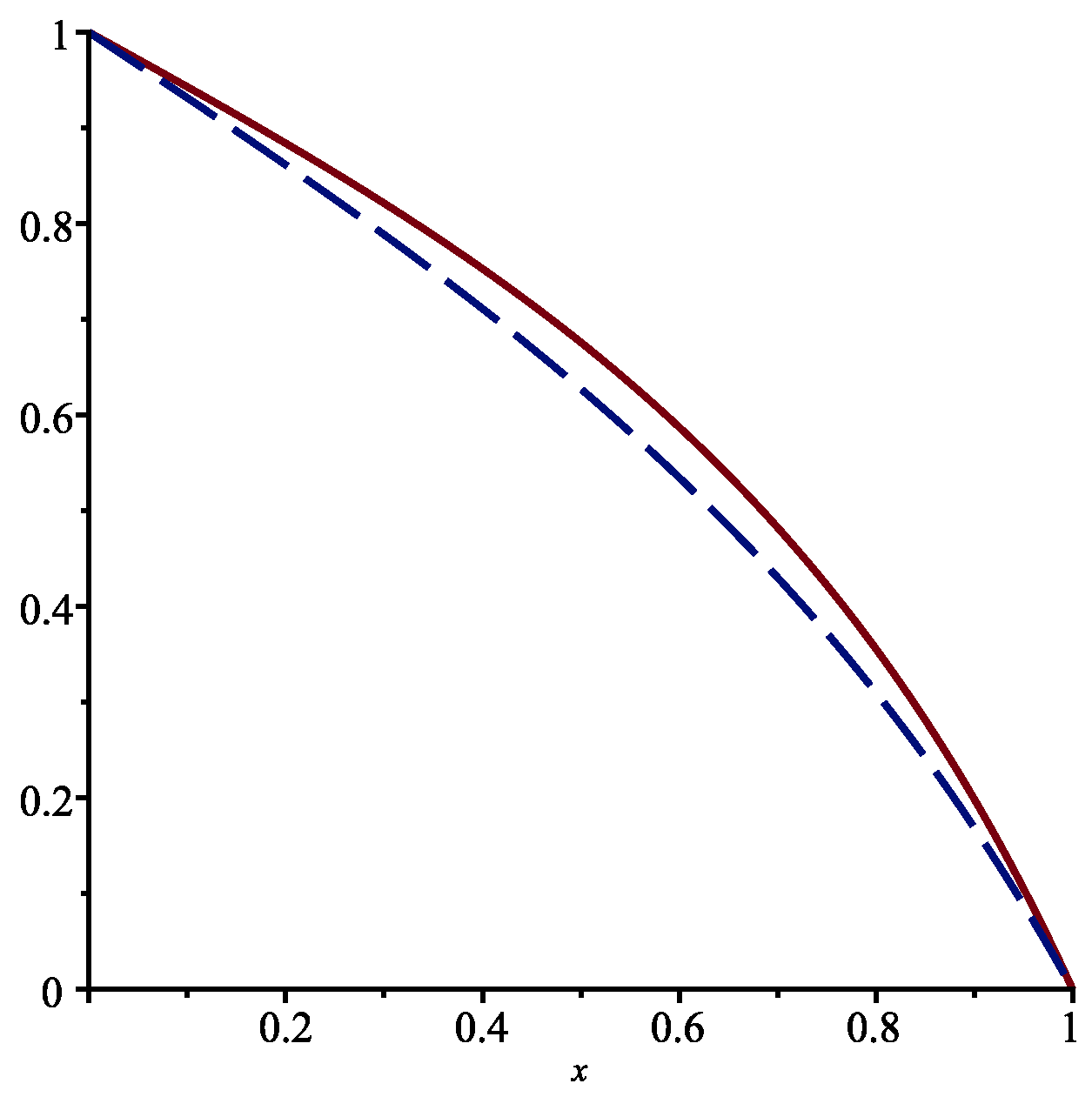
The solution that satisfies the boundary conditions $p_0\left(0\right)=1$ and $p_0\left(1\right)=0$ is the straight line $p_0\left(x\right)=1-x$. The functions $p_0\left(x\right)$ and $p\left(x\right)$ are shown in Figure 1. We see the effect of the jumps on the probability of absorption at the origin as follows: jumps increase the value of this probability, which is logical since jumps bring the process from its current position x to a random value whose mathematical expectation is equal to zero.

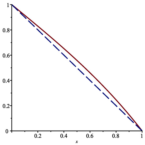
Figure 1. Functions $p\left(x\right)$ (full line) and $p_0\left(x\right)$ for $x\in [0,1]$ when $f\left(x\right)\equiv 0$ and $\sigma =\lambda =d=1$.

Next, we replace the function $f\left(x\right)\equiv 0$ by $f\left(x\right)=-\beta x$, where $\beta >0$. This time, the continuous part of $\left\{X\right(t),t\ge 0\}$ is an Ornstein–Uhlenbeck process, which is a very important diffusion process for these applications. Equation (21) becomes (with $\sigma =1$)

$${\displaystyle \frac{1}{2}}x{p}^{‴}\left(x\right)+\left({\displaystyle \frac{1}{2}}-\beta x^2\right)p^{″}\left(x\right)-(2\beta x+\lambda x)p^{\prime }\left(x\right)=0.$$

(32)

The general solution of this ODE can be expressed in terms of the Meijer G function and a generalized hypergeometric function. In the special case when $\beta =\lambda =1$, we find (with the help of Maple) that

$$p\left(x\right)=1+{\displaystyle \frac{x{e}^{x^2/2}}{I_0(1/2)}}\left\{c_3\left[I_0(1/2)K_0(x^2/2)-K_0(1/2)I_0(x^2/2)\right]-e^{-1/2}{I}_0(x^2/2)\right\},$$

(33)

where $K_0(·)$ is a Bessel function which can be defined as follows for $x>0$:

$$K_0\left(x\right)={\int }_0^{\infty }cos(xsinh\left(t\right))\mathrm{d}t={\int }_0^{\infty }{\displaystyle \frac{cos\left(xt\right)}{\sqrt{t^2+1}}}\mathrm{d}t.$$

(34)

The above function is such that $p\left(0\right)=1$ and $p\left(1\right)=0$. Contrary to the previous case, we cannot set $c_3$ equal to zero. We could substitute this expression into the IDE (13) and try to determine the constant $c_3$ for which the IDE is satisfied. We can also proceed as follows: The unique solution to Equation (32) that satisfies the three conditions $p\left(0\right)=1$, $p(1/2)=r$ and $p\left(1\right)=0$ is

$$\begin{array}{ccc}p\left(x\right)\hfill & =\hfill & 1-{\displaystyle \frac{x{e}^{x^2/2}{I}_0(x^2/2)\left[2e^{1/2}(r-1)K_0(1/2)+e^{1/8}{K}_0(1/8)\right]}{e^{5/8}\left[I_0(1/2)K_0(1/8)-K_0(1/2)I_0(1/8)\right]}}\hfill \\ \hfill & \hfill & +{\displaystyle \frac{x{e}^{x^2/2}{K}_0(x^2/2)\left[2e^{1/2}(r-1)I_0(1/2)+e^{1/8}{I}_0(1/8)\right]}{e^{5/8}\left[I_0(1/2)K_0(1/8)-K_0(1/2)I_0(1/8)\right]}}.\hfill \end{array}$$

(35)

Substituting this function into Equation (13), we find that the constant r is approximately equal to 0.676.

Proposition 3. 

The function $p\left(x\right)$ when $f\left(x\right)=-x$ and $\sigma =\lambda =d=1$ is given by

$$\begin{array}{ccc}p\left(x\right)\hfill & =\hfill & 1-{\displaystyle \frac{x{e}^{x^2/2}{I}_0(x^2/2)\left[-0.648e^{1/2}{K}_0(1/2)+e^{1/8}{K}_0(1/8)\right]}{e^{5/8}\left[I_0(1/2)K_0(1/8)-K_0(1/2)I_0(1/8)\right]}}\hfill \\ \hfill & \hfill & +{\displaystyle \frac{x{e}^{x^2/2}{K}_0(x^2/2)\left[-0.648e^{1/2}{I}_0(1/2)+e^{1/8}{I}_0(1/8)\right]}{e^{5/8}\left[I_0(1/2)K_0(1/8)-K_0(1/2)I_0(1/8)\right]}}\hfill \end{array}$$

(36)

for $x\in [0,1]$.

Remark 3. 

Making use of Maple’s evalf function, we can rewrite the function $p\left(x\right)$ as follows:

$$p\left(x\right)\approx 1-0.5708x{e}^{x^2}{I}_0(x^2/2)+0.0005217x{e}^{x^2/2}{K}_0(x^2/2).$$

(37)

With $\lambda =0$, we must solve the ODE

$${\displaystyle \frac{1}{2}}{p}_0^{″}\left(x\right)-x{p}_0^{\prime }\left(x\right)=0.$$

(38)

We find that

$$p_0\left(x\right)=1-{\displaystyle \frac{\mathrm{erf}\left(ix\right)}{\mathrm{erf}\left(i\right)}},$$

(39)

where erf$(·)$ is the error function defined by

$$\mathrm{erf}\left(x\right)={\displaystyle \frac{2}{\sqrt{\pi }}}{\int }_0^x{e}^{-t^2}\mathrm{d}t.$$

(40)

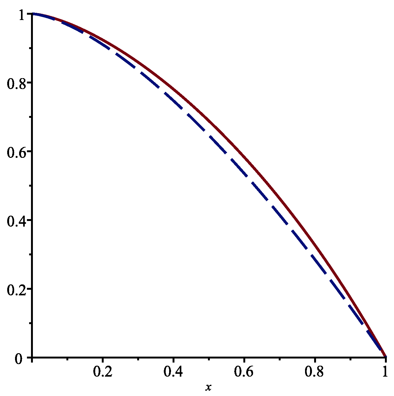
Figure 2 presents the functions $p\left(x\right)$ and $p_0\left(x\right)$ in the interval $[0,1]$.

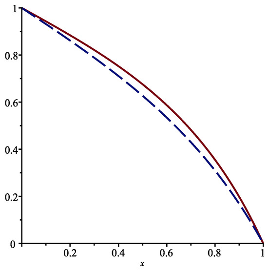
Figure 2. Functions $p\left(x\right)$ (full line) and $p_0\left(x\right)$ for $x\in [0,1]$ when $f\left(x\right)=-x$ and $\sigma =\lambda =d=1$.

Finally, we consider the jump-diffusion process defined by

$$X\left(t\right)=X\left(0\right)+{\int }_0^t{\displaystyle \frac{\gamma -1}{2X\left(s\right)}}\mathrm{d}s+\sigma B\left(t\right)+\sum _{i=0}^{N\left(t\right)}{Y}_i,$$

(41)

where $\gamma \in [0,2)$. As mentioned above, the continuous part of $\left\{X\right(t),t\ge 0\}$ is a Bessel process that can attain the origin. Since the origin is actually a regular boundary for this process (see [4]), we can consider it in the interval $(-\infty ,\infty )$. The Bessel process plays an important role in financial mathematics.

Let us take $\gamma =1/2$ and $\sigma =d=1$. In the absence of jumps, the function $p_0\left(x\right)$ satisfies the ODE

$${\displaystyle \frac{1}{2}}{p}_0^{″}\left(x\right)-{\displaystyle \frac{1}{4x}}{p}_0^{\prime }\left(x\right)=0.$$

(42)

With $p_0\left(0\right)=1$ and $p_0\left(1\right)=0$, we find that

$$p_0\left(x\right)=1-x^{3/2}.$$

(43)

When $\lambda =1$, we must solve the third-order linear ODE

$${\displaystyle \frac{1}{2}}x{p}^{‴}\left(x\right)+{\displaystyle \frac{1}{4}}{p}^{″}\left(x\right)-x{p}^{\prime }\left(x\right)=0.$$

(44)

The software program Maple provides the following solution that is such that $p\left(0\right)=1$, $p(1/2)=r$ and $p\left(1\right)=0$:

$$\begin{array}{ccc}\hfill p\left(x\right)& =& 1+{\displaystyle \frac{1}{\mathrm{\Delta }}}\{-x[4(r-1)\mathrm{hypergeom}\left(\left[{\displaystyle \frac{3}{4}}\right],\left[{\displaystyle \frac{5}{4}},{\displaystyle \frac{7}{4}}\right],{\displaystyle \frac{1}{2}}\right)\hfill \\ & & +\sqrt{2}\mathrm{hypergeom}\left(\left[{\displaystyle \frac{3}{4}}\right],\left[{\displaystyle \frac{5}{4}},{\displaystyle \frac{7}{4}}\right],{\displaystyle \frac{1}{8}}\right)]\mathrm{hypergeom}\left(\left[{\displaystyle \frac{1}{2}}\right],\left[{\displaystyle \frac{3}{4}},{\displaystyle \frac{3}{2}}\right],{\displaystyle \frac{x^2}{2}}\right)\hfill \\ & & +x^{3/2}[4(r-1)\mathrm{hypergeom}\left(\left[{\displaystyle \frac{1}{2}}\right],\left[{\displaystyle \frac{3}{4}},{\displaystyle \frac{3}{2}}\right],{\displaystyle \frac{1}{2}}\right)\hfill \\ & & +2\mathrm{hypergeom}\left(\left[{\displaystyle \frac{1}{2}}\right],\left[{\displaystyle \frac{3}{4}},{\displaystyle \frac{3}{2}}\right],{\displaystyle \frac{1}{8}}\right)\left]\mathrm{hypergeom}\left(\left[{\displaystyle \frac{3}{4}}\right],\left[{\displaystyle \frac{5}{4}},{\displaystyle \frac{7}{4}}\right],{\displaystyle \frac{x^2}{2}}\right)\right\},\hfill \end{array}$$

(45)

where

$$\begin{array}{ccc}\hfill \mathrm{\Delta }& :=& \sqrt{2}\mathrm{hypergeom}\left(\left[{\displaystyle \frac{3}{4}}\right],\left[{\displaystyle \frac{5}{4}},{\displaystyle \frac{7}{4}}\right],{\displaystyle \frac{1}{8}}\right)\mathrm{hypergeom}\left(\left[{\displaystyle \frac{1}{2}}\right],\left[{\displaystyle \frac{3}{4}},{\displaystyle \frac{3}{2}}\right],{\displaystyle \frac{1}{2}}\right)\hfill \\ & & -2\mathrm{hypergeom}\left(\left[{\displaystyle \frac{3}{4}}\right],\left[{\displaystyle \frac{5}{4}},{\displaystyle \frac{7}{4}}\right],{\displaystyle \frac{1}{2}}\right)\mathrm{hypergeom}\left(\left[{\displaystyle \frac{1}{2}}\right],\left[{\displaystyle \frac{3}{4}},{\displaystyle \frac{3}{2}}\right],{\displaystyle \frac{1}{8}}\right)\hfill \end{array}$$

(46)

and hypergeom is the generalized hypergeometric function, which is defined in Maple by

$$\mathrm{hypergeom}([n_1,n_2,\dots ],[d_1,d_2,\dots ],z)=\sum _{k=0}^{\infty }{\displaystyle \frac{z^k{\prod }_{i=1}^p\mathrm{pochhammer}(n_i,k)}{k!{\prod }_{j=1}^q\mathrm{pochhammer}(d_j,k)}}$$

(47)

with

$$\mathrm{pochhammer}(z,n):=z(z+1)\cdots (z+n-1).$$

(48)

The generalized hypergeometric function is often denoted by ${}_{p}F_q(n,d,z)$. Using this notation, we would write

$$\mathrm{hypergeom}\left(\left[{\displaystyle \frac{3}{4}}\right],\left[{\displaystyle \frac{5}{4}},{\displaystyle \frac{7}{4}}\right],{\displaystyle \frac{1}{2}}\right)={}_{1}F_2\left({\displaystyle \frac{3}{4}};{\displaystyle \frac{5}{4}},{\displaystyle \frac{7}{4}};{\displaystyle \frac{1}{2}}\right),$$

(49)

etc.

When we substitute the function $p\left(x\right)$ defined in Equation (45) into Equation (13), we find that the IDE is satisfied if we take $r\approx 0.688$.

Proposition 4. 

The probability $P\left[X\right(\tau \left(x\right))=0]$ when $f\left(x\right)=-{\displaystyle \frac{1}{4x}}$ and $\sigma =\lambda =d=1$ is the function $p\left(x\right)$ given in Equation (45) for $x\in [0,1]$, with $r\approx 0.688$.

The functions $p\left(x\right)$ and $p_0\left(x\right)$ in the interval $[0,1]$ are displayed in Figure 3.

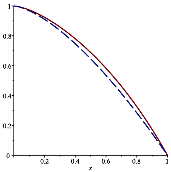
Figure 3. Functions $p\left(x\right)$ (full line) and $p_0\left(x\right)$ for $x\in [0,1]$ when $f\left(x\right)=-{\displaystyle \frac{1}{4x}}$ and $\sigma =\lambda =d=1$.

As we have seen in this section, the problem of calculating the probability $p\left(x\right)=P\left[X\right(\tau \left(x\right))=0]$, which is straightforward in the case of diffusion processes without jumps, becomes very difficult when jumps according to a Poisson process are added. In the next section, we will use numerical methods to obtain the mean $m\left(x\right)$ of the random variable $\tau \left(x\right)$ and its moment-generating function $M(x;\alpha )$.

3. Numerical Solutions

In this section, we present the numerical solution of integro-differential Equation (12) as follows:

$${\displaystyle \frac{1}{2}}{\sigma }^2{m}^{″}\left(x\right)+f\left(x\right)m^{\prime }\left(x\right)+\lambda \left\{{\displaystyle \frac{1}{x}}{\int }_0^{x}m\left(z\right)\mathrm{d}z-m\left(x\right)\right\}=-1,$$

(50)

subject to the boundary conditions

$$m\left(0\right)=0,m\left(d\right)=0,$$

(51)

and Equation (11) as follows:

$${\displaystyle \frac{1}{2}}{\sigma }^2{M}^{″}\left(x\right)+f\left(x\right)M^{\prime }\left(x\right)+\lambda \left\{{\displaystyle \frac{1}{x}}{\int }_0^{x}M\left(z\right)\mathrm{d}z-M\left(x\right)\right\}=\alpha M\left(x\right),$$

(52)

subject to the boundary conditions

$$M\left(0\right)=1,M\left(d\right)=1.$$

(53)

The function $f\left(x\right)$ takes different forms; more specifically, we will treat the following special cases:

$$f\left(x\right)=\left\{\begin{array}{c}0,\hfill \\ -\beta x,\hfill \\ {\displaystyle \frac{\gamma -1}{2x}}.\hfill \end{array}\right.$$

(54)

The parameters values are taken to be $\beta =\sigma =d=1$, $\gamma ={\displaystyle \frac{1}{2}}$, and various values of $\alpha \in (0,1]$.

We employ finite difference methods for spatial discretization and iterative correction to account for the integral term (see [23]). The numerical results demonstrate the behaviour of the functions $m\left(x\right)$ and $M\left(x\right)$ for two values of parameter $\lambda$, namely 0 and 1.

3.1. Discretization of the Domain

The computational domain is defined as $x\in [0,1]$, which is discretized into N equally spaced points as follows:

$$x_i={\displaystyle \frac{i}{N-1}},i=0,1,\dots ,N-1,$$

(55)

where the grid spacing is given by $dx=x_{i+1}-x_i$.

3.2. Finite Difference Approximations

To approximate the derivatives in each equation, we use the following central finite difference scheme:

-

The second derivative is approximated as

$${\displaystyle \frac{{\mathrm{d}}^{2}y}{\mathrm{d}{x}^2}}\approx {\displaystyle \frac{y_{i+1}-2y_i+y_{i-1}}{d{x}^2}}.$$

(56)

-

The first derivative is approximated as

$${\displaystyle \frac{\mathrm{d}y}{\mathrm{d}x}}\approx {\displaystyle \frac{y_{i+1}-y_{i-1}}{2dx}}.$$

(57)

These approximations are used to construct the system matrix.

3.3. Integral Term Approximation

The integral term in the equation is given by

$$I\left(x\right)={\int }_0^{x}y\left(z\right)\mathrm{d}z.$$

(58)

We approximate it numerically using the trapezoidal rule, as follows:

$$I\left(x_i\right)\approx \sum _{j=0}^{i-1}{\displaystyle \frac{y_j+y_{j+1}}{2}}dx.$$

(59)

This is efficiently computed using MATLAB’s built-in ‘cumtrapz()’ function (version R2023b).

3.4. Construction of the System of Equations

By discretizing the given equation, we obtain the following linear system:

$$\mathbf{A}\mathbf{y}=\mathbf{b},$$

(60)

where $\mathbf{A}$ is a coefficient matrix incorporating the finite difference terms, and $\mathbf{b}$ is the right-hand side vector.

3.5. Iterative Approach for the Integral Term

Since $I\left(x\right)$ depends on $y\left(x\right)$, we employ an iterative correction scheme as follows:

• Start with an initial guess $y\left(x\right)=0$.
• Compute the integral term $I\left(x\right)$.
• Update the right-hand side $\mathbf{b}$ using $I\left(x\right)$.
• Solve for $y\left(x\right)$.
• Repeat until convergence is achieved.

3.6. Graphs

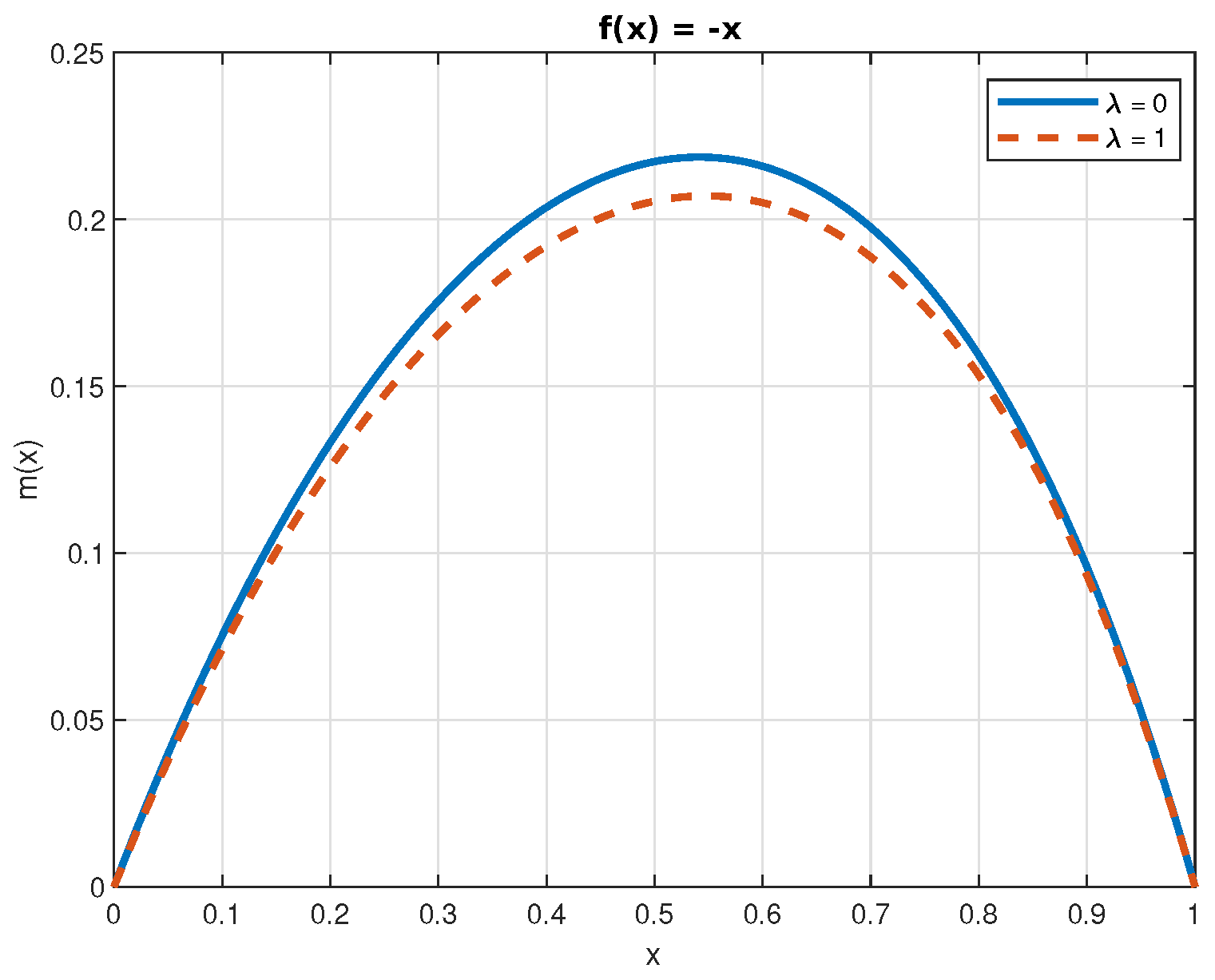
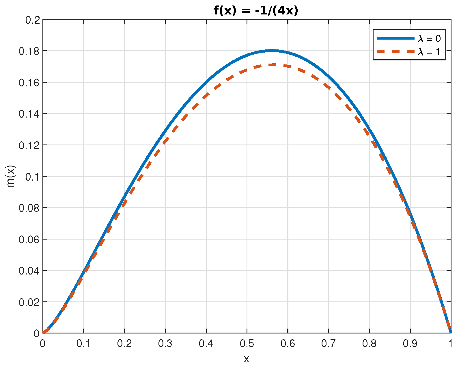
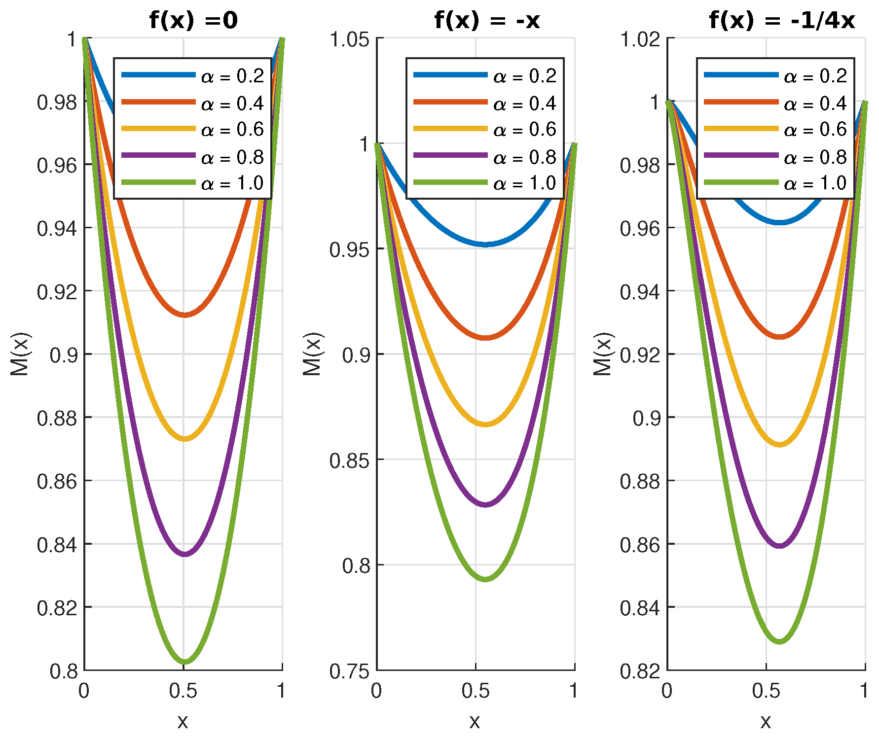
The numerical solutions of Equations (50) and (52) are displayed in Figure 4, Figure 5, Figure 6, Figure 7 and Figure 8. In the case of the function $m\left(x\right)$, we can see that the jumps decrease its value. This is a consequence of the fact that jumps bring the process closer, on average, to the origin. Finally, because $\alpha >0$, the effect of the jumps on the function $M(x;\alpha )$ is the opposite.

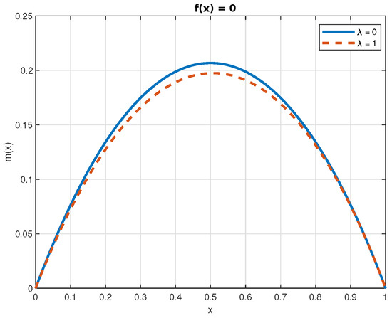
Figure 4. Function $m\left(x\right)$ for $f\left(x\right)=0$, with $\lambda =0.1$.

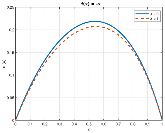
Figure 5. Function $m\left(x\right)$ for $f\left(x\right)=-x$, with $\lambda =0.1$.

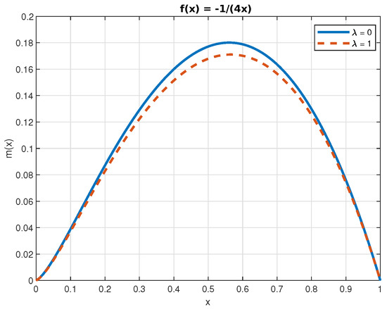
Figure 6. The function $m\left(x\right)$ for $f\left(x\right)={\displaystyle \frac{-1}{4x}}$, with $\lambda =0.1$.

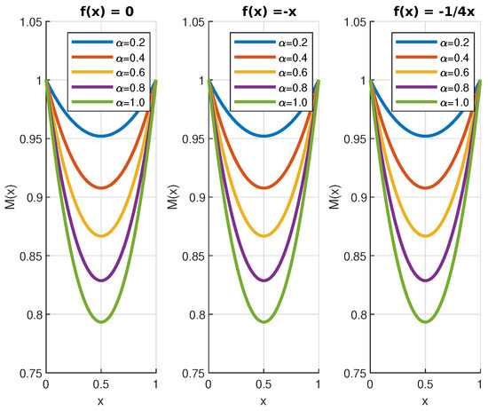
Figure 7. Function $M\left(x\right)$ for $f\left(x\right)=0,-x$ and ${\displaystyle \frac{-1}{4x}}$ with $\lambda =0$ and for different values of $\alpha$.

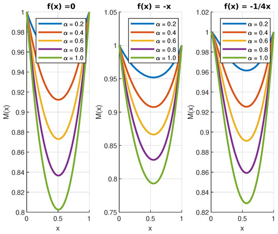
Figure 8. Function $M\left(x\right)$ for $f\left(x\right)=0,-x$ and ${\displaystyle \frac{-1}{4x}}$ with $\lambda =1$ and for different values of $\alpha$.

4. Discussion

To obtain more realistic models, many authors nowadays add jumps to diffusion processes according to a Poisson process such as a Brownian motion process. From a mathematical point of view, this entails that problems such as calculating the characteristics of random variables called first-hitting times become much more difficult.

Indeed, as we have seen in this paper, rather than solving linear ordinary differential equations, the introduction of jumps whose size is a continuous random variable implies that we now have to solve integro-differential equations.

In this paper, we considered such a problem in the case when the jump size is uniformly distributed on the interval $(-2x,0)$ (when $x>0$), where x is the current value of the process. We were able to obtain exact analytical expressions, in terms of special functions, for the probability that the jump-diffusion process $\left\{X\right(t),t\ge 0\}$ will hit the origin before a barrier at $x=1$. Three particular cases for the continuous part of $\left\{X\right(t),t\ge 0\}$ were treated. These three cases are among the most important ones for applications.

In Section 3, we presented numerical solutions to the integro-differential equations that must be solved, subject to the appropriate boundary conditions, to obtain the mean and the moment-generating function of the first-hitting time of interest.

There are still few papers with explicit results for this type of problem. Here, we were able to transform the integro-differential equations into third-order ordinary differential equations. These equations are linear, but with non-constant coefficients. Therefore, their solutions are often quite intricate. Moreover, even if we are able to solve them explicitly, we still have to substitute the solutions into the original integro-differential equations to determine the value of the third arbitrary constant in the general solutions.

The main difficulty in obtaining explicit and exact analytical results for the type of problems studied in this paper is thus solving the ODEs. We were able to do this for the function $p\left(x\right)$, but in the case of the functions $m\left(x\right)$ and $M(x;\alpha )$, we had to resort to numerical methods.

As a continuation of this work, we could consider jump-diffusion processes in two or more dimensions. Sometimes, by using symmetry, it is possible to reduce these problems to one-dimensional problems. Another possibility would be to consider jumps whose size is a discrete, rather than a continuous, random variable. In this case, instead of integro-differential equations, we would have to solve difference-differential equations.

References

- Øksendal, B. Stochastic Differential Equations; Springer: Berlin/Heidelberg, Germany, 2003. [Google Scholar] [CrossRef]
- Cox, D.R.; Miller, H.D. The Theory of Stochastic Processes; Methuen: London, UK, 1965. [Google Scholar]
- Kou, S.G.; Wang, H. First passage times of a jump diffusion process. Adv. Appl. Probab. 2003, 35, 504–531. [Google Scholar] [CrossRef]
- Karlin, S.; Taylor, H.M. A Second Course in Stochastic Processes; Academic Press: New York, NY, USA, 1981. [Google Scholar]
- Uhlenbeck, G.E.; Ornstein, L.S. On the theory of the Brownian motion. Phys. Rev. 1930, 36, 823–841. [Google Scholar] [CrossRef]
- Revuz, D.; Yor, M. Continuous Martingales and Brownian Motion; Springer: Berlin/Heidelberg, Germany, 1991. [Google Scholar] [CrossRef]
- Lefebvre, M. Applied Stochastic Processes; Springer: New York, NY, USA, 2007. [Google Scholar] [CrossRef]
- Lefebvre, M. Exit problems for jump-diffusion processes with uniform jumps. J. Stoch. Anal. 2020, 1, 5. [Google Scholar] [CrossRef]
- Lefebvre, M. Exact solutions to first-passage problems for jump-diffusion processes. Bull. Pol. Acad. Sci. Math. 2024, 72, 81–95. [Google Scholar] [CrossRef]
- Merton, R.C. Option pricing when underlying stock returns are discontinuous. J. Financ. Econ. 1976, 3, 125–144. [Google Scholar] [CrossRef]
- Abundo, M. On first-passage times for one-dimensional jump-diffusion processes. Probab. Math. Statist. 2000, 20, 399–423. [Google Scholar]
- Abundo, M. On the first hitting time of a one-dimensional diffusion and a compound Poisson process. Methodol. Comput. Appl. Probab. 2010, 12, 473–490. [Google Scholar] [CrossRef]
- Cai, N. On first passage times of a hyper-exponential jump diffusion process. Oper. Res. Lett. 2009, 37, 127–134. [Google Scholar] [CrossRef]
- Peng, J.; Liu, Z. First passage time moments of jump-diffusions with Markovian switching. Int. J. Stoch. Anal. 2011, 501360. [Google Scholar] [CrossRef]
- Yin, C.; Shen, Y.; Wen, Y. Exit problems for jump processes with applications to dividend problems. J. Comput. Appl. Math. 2013, 245, 30–52. [Google Scholar] [CrossRef]
- Zhou, J.; Wu, L. Occupation times of refracted double exponential jump diffusion processes. Stat. Probab. Lett. 2015, 106, 218–227. [Google Scholar] [CrossRef]
- Ai, M.; Zhang, Z.; Yu, W. First passage problems of refracted jump diffusion processes and their applications in valuing equity-linked death benefits. J. Ind. Manag. Optim. 2022, 18, 1689–1707. [Google Scholar] [CrossRef]
- Abundo, M. On the first-passage area of a one-dimensional jump-diffusion process. Methodol. Comput. Appl. Probab. 2013, 15, 85–103. [Google Scholar] [CrossRef]
- Lefebvre, M. Exact solution to a first-passage problem for an Ornstein-Uhlenbeck process with jumps and its integral. Stat. Probab. Lett. 2024, 205, 109956. [Google Scholar] [CrossRef]
- Evans, M.R.; Majumdar, S.N. Diffusion with stochastic resetting. Phys. Rev. Lett. 2011, 106, 160601. [Google Scholar] [CrossRef] [PubMed]
- Abundo, M. The first-passage area of Wiener process with stochastic resetting. Methodol. Comput. Appl. Probab. 2023, 25, 92. [Google Scholar] [CrossRef]
- Abramowitz, M.; Stegun, I.A. Handbook of Mathematical Functions: With Formulas, Graphs, and Mathematical Tables; Dover Publications: New York, NY, USA, 1965. [Google Scholar]
- Darania, P.; Ebadian, A. A method for the numerical solution of the integro-differential equations. Appl. Math. Comput. 2007, 188, 657–668. [Google Scholar] [CrossRef]
Disclaimer/Publisher’s Note: The statements, opinions and data contained in all publications are solely those of the individual author(s) and contributor(s) and not of MDPI and/or the editor(s). MDPI and/or the editor(s) disclaim responsibility for any injury to people or property resulting from any ideas, methods, instructions or products referred to in the content. |
© 2025 by the authors. Licensee MDPI, Basel, Switzerland. This article is an open access article distributed under the terms and conditions of the Creative Commons Attribution (CC BY) license (https://creativecommons.org/licenses/by/4.0/).