Bayesian Tapered Narrowband Least Squares for Fractional Cointegration Testing in Panel Data

Abstract

Fractional cointegration has been extensively examined in time series analysis, but its extension to heterogeneous panel data with unobserved heterogeneity and cross-sectional dependence remains underdeveloped. This paper develops a robust framework for testing fractional cointegration in heterogeneous panel data, where unobserved heterogeneity, cross-sectional dependence, and persistent shocks complicate traditional approaches. We propose the Bayesian Tapered Narrowband Least Squares (BTNBLS) estimator, which addresses three critical challenges: (1) spectral leakage in long-memory processes, mitigated via tapered periodograms; (2) precision loss in fractional parameter estimation, resolved through narrowband least squares; and (3) unobserved heterogeneity in cointegrating vectors (${\theta }_i$) and memory parameters ($\nu ,\delta$), modeled via hierarchical Bayesian priors. Monte Carlo simulations demonstrate that BTNBLS outperforms conventional estimators (OLS, NBLS, TNBLS), achieving minimal bias (0.041–0.256), near-nominal coverage probabilities (0.87–0.94), and robust control of Type 1 errors (0.01–0.07) under high cross-sectional dependence ($\rho =0.8$), while the Bayesian Chen–Hurvich test attains near-perfect power (up to 1.00) in finite samples. Applied to Purchasing Power Parity (PPP) in 18 fragile Sub-Saharan African economies, BTNBLS reveals statistically significant fractional cointegration between exchange rates and food price ratios in 15 countries ($p<0.05$), with a pooled estimate ($\widehat{\theta }=0.33$, $p<0.001$) indicating moderate but resilient long-run equilibrium adjustment. These results underscore the importance of Bayesian shrinkage and spectral tapering in panel cointegration analysis, offering policymakers a reliable tool to assess persistence of shocks in institutionally fragmented markets.

1. Introduction

Although cointegration techniques have long been pivotal in economic and financial research to model equilibrium relationships among nonstationary variables, traditional methods impose restrictive assumptions on integration orders and linear dynamics. Fractional cointegration addresses these limitations by accommodating non-integer integration and persistent nonlinear dependencies, offering a more flexible framework for real-world time series. However, extending these advances to panel data where unobserved heterogeneity, cross-sectional dependencies, and structural variations complicate inference remains underexplored. Existing frequentist approaches for fractional cointegration in panels, such as adaptations of time series tests, often struggle to account for parameter variability across units or adequately model fixed effects, risking biased estimates and spurious conclusions [1,2,3,4,5].

Recent methodological innovations, including tapered periodograms to mitigate spectral leakage and narrowband least squares for precise estimation of fractional parameters, have improved time series analysis [6,7,8]. However, their integration into panel frameworks, particularly in Bayesian paradigms, has lagged. Bayesian methods, with their inherent capacity to model uncertainty and heterogeneity through hierarchical structures, present a promising avenue for addressing these challenges. Previous work by Olaniran and Ismail [3], Olaniran et al. [4,5] demonstrated the feasibility of adapting time series fractional cointegration tests, such as Chen and Hurvich [9], to panel settings, but highlighted residual limitations in handling cross-unit heterogeneity and boundary effects. Meanwhile, Leschinski et al. [8] underscored the fragility of conventional tests in small samples, emphasizing the need for robust adaptive methodologies.

This paper introduces Bayesian Tapered Narrowband Least Squares (BTNBLS), a novel methodological framework designed to address longstanding challenges in testing fractional cointegration within panel data settings characterized by fixed effects, cross-sectional heterogeneity, and persistent shocks. Traditional approaches to cointegration analysis, largely confined to integer-order integration and time series contexts, struggle to accommodate the nuanced dynamics of panel data, where unobserved heterogeneity and cross-unit variability often obscure long-run equilibria. Departing from conventional frequentist methods, BTNBLS pioneers a nonparametric Bayesian hierarchical model that jointly estimates unit-specific cointegrating vectors (${\theta }_i$) and fractional integration parameters (${\nu }_i,{\delta }_i$), explicitly modeling cross-sectional disparities in persistence and equilibrium adjustment. By integrating tapered periodograms, which mitigate boundary distortions in spectral estimation through cosine-weighted data smoothing, with narrowband least squares that isolate low-frequency components of the spectrum, the framework sharpens precision in identifying fractional cointegrating relationships. This dual innovation reduces spectral leakage and attenuates bias in memory parameter estimation, particularly in panels with moderate to strong error correlations, where traditional estimators like OLS and NBLS falter due to endogeneity and variance inflation. In addition, to illustrate its practical applicability, the paper presents an empirical application of BTNBLS to test the purchasing power parity (PPP) hypothesis in 18 fragile Sub-Saharan African countries. The PPP hypothesis posits that exchange rates and price ratios should move in tandem over the long run, reflecting a stable relationship between currencies and price levels. Traditional cointegration tests often fail to detect such relationships, particularly in datasets characterized by fractional integration and heterogeneity. However, BTNBLS reveals a fractional cointegrating relationship between exchange rates and price ratios in these countries, a finding that had been obscured by conventional methods. This empirical result underscores the framework’s ability to uncover subtle yet significant economic relationships that might otherwise go unnoticed.

2. Related Work

The study of cointegration originated with the seminal work of Engle and Granger [10], who introduced both standard (integer-order) and fractional cointegration frameworks. While standard cointegration has dominated econometric research, recent years have seen growing interest in fractional cointegration, driven by its ability to model nonlinear dynamics and persistent dependencies through non-integer memory parameters $\delta$ and $\nu$ [6,9]. However, extensions to panel data that integrate cross-sectional and temporal dimensions to enhance inferential power [11] remain sparse, particularly in settings with unobserved heterogeneity or fixed effects.

Early advances in fractional cointegration focused on time series data. For example, Robinson [12] and Marinucci and Robinson [13] developed narrowband least squares estimators (NBLSE) in the frequency domain to address inconsistencies in ordinary least squares (OLS) under correlated regressors and errors. These methods were refined by Chen and Hurvich [14], who introduced tapered estimators to mitigate boundary effects and polynomial trends. However, such approaches were confined to bivariate systems or single cointegrating ranks, limiting their applicability to multivariate or panel settings.

Chen and Hurvich [9] advanced the field with a multivariate model of common components, which allows memory parameters to vary between orthogonal subspaces. Their residual-based test, utilizing Gaussian semiparametric estimation, became a benchmark for time series. Yet, adaptations to panel data faced challenges: cross-sectional heterogeneity, fixed effects, and structural disparities between units were often overlooked. Ergemen and Velasco [15] pioneered panel frameworks with fractionally integrated errors and fixed effects, employing Monte Carlo simulations to validate their approach. However, their reliance on frequentist methods left unresolved the need to model parameter variability across units, a gap later highlighted by Olaniran and Ismail [3], Olaniran et al. [4,5], Leschinski et al. [8], who collectively demonstrated the fragility of residual-based tests under cross-sectionally correlated short-run dynamics.

Recent efforts to bridge these gaps include Monge et al. [16], Malmierca-Ordoqui et al. [17], Diakodimitriou et al. [18] and Olaniran et al. [4,5], who adapted Chen and Hurvich’s [9] test to fixed effects panels. While their modified test accommodated moderate heterogeneity, it retained limitations in handling spectral leakage and boundary distortions, issues previously addressed in time series via tapered periodograms [6] and narrowband techniques [13]. Notably, Bayesian methods, which inherently model uncertainty through hierarchical priors and accommodate unit-specific parameters, have been underexplored in panel fractional cointegration. Prior Bayesian works on standard cointegration (non-fractional) (e.g., Koop et al. [19]) focused on time series and Koop et al. [20] for panel data leaving fractional panel applications underdeveloped.

The integration of tapered estimators into Bayesian frameworks offers promise. For example, Shaby and Ruppert [21] combined tapering with nonparametric Bayesian models to mitigate nonstationarity in univariate series, while Selvaraj et al. [22] employed narrowband least squares in wavelet-based Bayesian analyses. However, these innovations have yet to coalesce into a unified panel data methodology. Existing tests, such as those of Caporale and Gil-Alana [23,24], Wang et al. [25], Olayeni et al. [26] and Pata and Yilanci [27], Demetrescu et al. [28], Caporale et al. [29], Uche et al. [30], either lack robustness to cross-sectional heterogeneity or assume homogeneity in cointegrating vectors, a restrictive premise in real-world datasets.

This paper addresses these gaps by unifying three strands of research: (1) tapered narrowband estimation for spectral precision, (2) Bayesian nonparametrics for modeling cross-unit variability, and (3) panel cointegration frameworks accommodating fixed effects. Building on Olaniran and Ismail [3], Olaniran et al. [4,5], we extend Chen and Hurvich’s [9] test into a Bayesian paradigm, incorporating tapered periodograms to suppress boundary effects and narrowband least squares to refine memory parameter estimation. Our approach diverges from frequentist panel methods (e.g., Ergemen [31]) by explicitly modeling heterogeneity in cointegrating vectors and fractional parameters through hierarchical priors, thereby advancing the detection of long-run equilibria in complex and heterogeneous panels.

3. Bayesian Tapered Narrowband Least Squares

We extend the fixed effect panel model of Chen and Hurvich [9] to a Bayesian hierarchical framework to address cross-sectional heterogeneity and spectral leakage. Let $y_{it}=u_{it}-{\alpha }_i$ and $x_{it}=v_{it}$ denote the demeaned dependent and independent variables for unit i at time t, where ${\alpha }_i$ are unit-specific fixed effects. The system is defined as:

$$\begin{array}{cc}\hfill y_{it}& ={\theta }_i{x}_{it}+{(1-L)}^{-\delta }{ϵ}_{1,it},\hfill \\ \hfill x_{it}& ={(1-L)}^{-\nu }{ϵ}_{2,it},\hfill \end{array}$$

(1)

where L is the lag operator such that $L^k{x}_{it}=x_{i,t-k}$, ${(1-L)}^{-\nu }$ is the fractional differencing operator defined via the binomial expansion:

$${(1-L)}^{-\nu }=\sum _{k=0}^{\infty }{\displaystyle \frac{\Gamma (k+\nu )}{\Gamma \left(\nu \right)\Gamma (k+1)}}{L}^k,$$

where $\Gamma (·)$ is the gamma function.

-

${ϵ}_{1,it}\sim \mathcal{N}(0,{\sigma }_{ϵ}^2)$ and ${ϵ}_{2,it}\sim \mathcal{N}(0,1)$ are independent innovation processes.

-

$\delta \in (0.5,1.5)$ and $\nu \in (0.5,1.5)$ are memory parameters satisfying $\nu >\delta$ under fractional cointegration.

The transformation $y_{it}=u_{it}-{\alpha }_i$ ensures that $\mathbb{E}\left[y_{it}\right]={\theta }_i\mathbb{E}\left[x_{it}\right]$, eliminating unit-specific intercepts. This avoids confounding cross-sectional heterogeneity with the cointegrating relationship.

3.1. Likelihood Construction

The likelihood is formulated in the frequency domain to leverage the spectral properties of fractionally integrated processes. For each unit i, define the tapered periodogram ${\mathbf{I}}_{yx,i}^{\prime }\left(m\right)$ at bandwidth m as:

$${\mathbf{I}}_{yx,i}^{\prime }\left(m\right)={\displaystyle \frac{1}{m}}\sum _{k=1}^m{\omega }_{y,i,k}^{\prime }{\overline{\omega }}_{x,i,k}^{\prime },$$

where ${\omega }_{y,i,k}^{\prime }$ and ${\omega }_{x,i,k}^{\prime }$ are tapered discrete Fourier transforms:

$${\omega }_{y,i,k}^{\prime }=\sum _{t=1}^T{q}_t^{p-1}{y}_{it}{e}^{-i{\lambda }_{k}t},{\lambda }_k={\displaystyle \frac{2\pi k}{T}}.$$

The taper $q_t^{p-1}={\displaystyle \frac{1}{2}}(1-e^{-i2\pi (t-1/2)s^{-1}})$ mitigates boundary effects by downweighting endpoints of the series.

The likelihood follows a complex Gaussian process:

$${\mathbf{I}}_{yx,i}^{\prime }\left(m\right)\sim \mathcal{CN}\left({\theta }_i{\mathbf{I}}_{xx,i}^{\prime }(m;\nu ),{\mathbf{F}}_{ϵϵ,i}^{\prime }(m;\delta )\right),$$

where:

-

${\mathbf{I}}_{xx,i}^{\prime }(m;\nu )={\displaystyle \frac{1}{m}}{\sum }_{k=1}^m{\left|{(1-e^{-i{\lambda }_k})}^{-\nu }\right|}^2$ is the tapered spectral density of $x_{it}$.

-

${\mathbf{F}}_{ϵϵ,i}^{\prime }(m;\delta )={\displaystyle \frac{1}{m}}{\sum }_{k=1}^m{\left|{(1-e^{-i{\lambda }_k})}^{-\delta }\right|}^2$ is the error spectral density.

3.2. Hierarchical Prior Specification

3.2.1. Unit-Specific Cointegrating Vectors

To pool information across units while preserving heterogeneity, we assume:

$${\theta }_i\sim \mathcal{N}\left({\mu }_{\theta },{\sigma }_{\theta }^2\right),i=1,\dots ,n,$$

with hyperpriors:

$${\mu }_{\theta }\sim \mathcal{N}(0,{\tau }^2),{\sigma }_{\theta }^{-2}\sim \mathrm{Gamma}(a,b).$$

The normal-gamma hierarchy ensures conjugacy, enabling closed-form posterior updates for ${\mu }_{\theta }$ and ${\sigma }_{\theta }^2$. The hyperparameter ${\tau }^2$ controls the shrinkage strength toward the global mean ${\mu }_{\theta }$.

3.2.2. Memory Parameters

To enforce $\nu >\delta$ (a necessary condition for cointegration), we specify:

$$\delta \sim {\mathrm{TruncNormal}}^{+}(0,{\varphi }^2),\nu \sim {\mathrm{TruncNormal}}^{+}(\delta +\eta ,{\varphi }^2),\eta >0,$$

where ${\mathrm{TruncNormal}}^{+}$ denotes a normal distribution truncated to $(0,\infty )$. The hyperparameter $\eta$ ensures a minimal gap between $\nu$ and $\delta$, avoiding near-degenerate cases.

3.2.3. Tapering Hyperparameters

The taper order p is modeled as:

$$p\sim \mathrm{Categorical}\left(\mathbf{q}\right),\mathbf{q}=(q_1,\dots ,q_P),$$

where $q_j={\displaystyle \frac{1}{2}}(1-e^{-i2\pi (j-1/2)s^{-1}})$ defines the taper weights. The categorical prior allows data-driven selection of the optimal taper to minimize spectral leakage.

3.3. Posterior Computation

The joint posterior distribution is:

$$p(\mathit{\theta },\delta ,\nu ,{\mu }_{\theta },{\sigma }_{\theta }^2\mid {\mathbf{I}}_{yx}^{\prime })\propto \prod _{i=1}^n\mathcal{CN}\left({\mathbf{I}}_{yx,i}^{\prime }\mid {\theta }_i{\mathbf{I}}_{xx,i}^{\prime },{\mathbf{F}}_{ϵϵ,i}^{\prime }\right)·p(\mathit{\theta },\delta ,\nu ,{\mu }_{\theta },{\sigma }_{\theta }^2).$$

Gibbs–Metropolis–Hastings Algorithm

Step 1: Sample ${\theta }_i$ The full conditional for ${\theta }_i$ combines the likelihood and prior:

$$p({\theta }_i\mid ·)\propto exp\left(-{\displaystyle \frac{1}{2}}\left[{\displaystyle \frac{{({\theta }_i-{\widehat{\theta }}_{\mathrm{TNBLS},i})}^2}{{\widehat{\sigma }}_{\theta ,i}^2}}+{\displaystyle \frac{{({\theta }_i-{\mu }_{\theta })}^2}{{\sigma }_{\theta }^2}}\right]\right),$$

where ${\widehat{\theta }}_{\mathrm{TNBLS},i}={\displaystyle \frac{\Re {\mathbf{I}}_{yx,i}^{\prime }}{{\mathbf{I}}_{xx,i}^{\prime }}}$ is the unit-specific TNBLS estimate, and ${\widehat{\sigma }}_{\theta ,i}^2={\mathbf{F}}_{ϵϵ,i}^{\prime }/{\mathbf{I}}_{xx,i}^{\prime }$. This is a normal distribution:

$${\theta }_i\mid ·\sim \mathcal{N}\left({\displaystyle \frac{{\widehat{\theta }}_{\mathrm{TNBLS},i}/{\widehat{\sigma }}_{\theta ,i}^2+{\mu }_{\theta }/{\sigma }_{\theta }^2}{1/{\widehat{\sigma }}_{\theta ,i}^2+1/{\sigma }_{\theta }^2}},{\left(1/{\widehat{\sigma }}_{\theta ,i}^2+1/{\sigma }_{\theta }^2\right)}^{-1}\right).$$

Step 2: Sample ${\mu }_{\theta },{\sigma }_{\theta }^2$ Using conjugacy:

$${\mu }_{\theta }\mid ·\sim \mathcal{N}\left({\displaystyle \frac{{\sum }_{i=1}^n{\theta }_i/{\sigma }_{\theta }^2}{n/{\sigma }_{\theta }^2+1/{\tau }^2}},{\left(n/{\sigma }_{\theta }^2+1/{\tau }^2\right)}^{-1}\right),$$

$${\sigma }_{\theta }^{-2}\mid ·\sim \mathrm{Gamma}\left(a+{\displaystyle \frac{n}{2}},b+{\displaystyle \frac{1}{2}}\sum _{i=1}^n{({\theta }_i-{\mu }_{\theta })}^2\right).$$

Step 1: Sample $\delta ,\nu$ via Metropolis–Hastings

• Proposal Distribution:

  $$q({\delta }^{\prime },{\nu }^{\prime }\mid \delta ,\nu )=\mathcal{N}(\delta ,{\varphi }^2)·\mathcal{N}(\nu ,{\varphi }^2)·\mathbb{I}({\nu }^{\prime }>{\delta }^{\prime }+\eta ).$$
• Acceptance Ratio:

  $$\alpha =min\left(1,{\displaystyle \frac{p({\mathbf{I}}_{yx}^{\prime }\mid {\delta }^{\prime },{\nu }^{\prime })·p\left({\delta }^{\prime }\right)p\left({\nu }^{\prime }\right)}{p({\mathbf{I}}_{yx}^{\prime }\mid \delta ,\nu )·p\left(\delta \right)p\left(\nu \right)}}·{\displaystyle \frac{q(\delta ,\nu \mid {\delta }^{\prime },{\nu }^{\prime })}{q({\delta }^{\prime },{\nu }^{\prime }\mid \delta ,\nu )}}\right).$$

Theorem 1 (Bias Reduction).

Under Assumptions A1–A4, the bias of the BTNBLS estimator satisfies:

$$\mathbb{E}\left[{\widehat{\theta }}_{BTNBLS}-{\theta }_0\right]=\mathcal{O}\left({\displaystyle \frac{1}{nT}}+{\displaystyle \frac{1}{\sqrt{m}}}\right),$$

which improves upon the bias of the TNBLS estimator, given by $\mathcal{O}\left({\displaystyle \frac{1}{\sqrt{nT}}}+{\displaystyle \frac{1}{\sqrt{m}}}\right)$. The assumptions are as follows:

• A1 (Stationarity): The memory parameters satisfy $\nu ,\delta \in (0.5,1.5)$, ensuring the process is nonstationary but mean-reverting.
• A2 (Spectral Smoothness): The tapered spectral density ${\mathbf{I}}_{xx,i}^{\prime }(m;\nu )$ is twice continuously differentiable with respect to ν.
• A3 (Prior Dominance): The hyperparameters satisfy ${\tau }^2=\mathcal{O}\left(n^{-1}\right)$, $a=\mathcal{O}\left(1\right)$, and $b=\mathcal{O}\left(1\right)$, ensuring that the prior does not asymptotically dominate the likelihood.
• A4 (Ergodicity): For each unit i, the process $\{x_{it},y_{it}\}$ is ergodic, with cross-sectional and temporal independence.

Proof. 

Let ${\widehat{\theta }}_{\mathrm{BTNBLS}}=\mathbb{E}[{\theta }_i\mid {\mathbf{I}}_{yx}^{\prime }]$. Decompose the bias as:

$$\mathbb{E}[{\widehat{\theta }}_{\mathrm{BTNBLS}}-{\theta }_0]=\underset{\mathrm{Shrinkage}\mathrm{Bias}}{\underbrace{\mathbb{E}[{\widehat{\theta }}_{\mathrm{BTNBLS}}-{\mu }_{\theta }]}}+\underset{\mathrm{Prior}\mathrm{Bias}}{\underbrace{\mathbb{E}[{\mu }_{\theta }-{\theta }_0]}}.$$

Step 1: Shrinkage Bias

From the posterior distribution of ${\theta }_i$:

$${\theta }_i\mid {\mathbf{I}}_{yx}^{\prime }\sim \mathcal{N}\left({\displaystyle \frac{{\widehat{\theta }}_{\mathrm{TNBLS},i}/{\widehat{\sigma }}_{\theta ,i}^2+{\mu }_{\theta }/{\sigma }_{\theta }^2}{1/{\widehat{\sigma }}_{\theta ,i}^2+1/{\sigma }_{\theta }^2}},{\left(1/{\widehat{\sigma }}_{\theta ,i}^2+1/{\sigma }_{\theta }^2\right)}^{-1}\right).$$

Taking expectations:

$$\mathbb{E}[{\theta }_i\mid {\mathbf{I}}_{yx}^{\prime }]={\displaystyle \frac{{\widehat{\theta }}_{\mathrm{TNBLS},i}/{\widehat{\sigma }}_{\theta ,i}^2+{\mu }_{\theta }/{\sigma }_{\theta }^2}{1/{\widehat{\sigma }}_{\theta ,i}^2+1/{\sigma }_{\theta }^2}}.$$

Subtracting ${\mu }_{\theta }$:

$$\mathbb{E}[{\theta }_i-{\mu }_{\theta }\mid {\mathbf{I}}_{yx}^{\prime }]={\displaystyle \frac{{\widehat{\theta }}_{\mathrm{TNBLS},i}-{\mu }_{\theta }}{1+{\widehat{\sigma }}_{\theta ,i}^2/{\sigma }_{\theta }^2}}.$$

By A3, ${\sigma }_{\theta }^2=\mathcal{O}\left(n^{-1}\right)$, and under ergodicity (A4), ${\widehat{\sigma }}_{\theta ,i}^2={\mathcal{O}}_p\left(1\right)$. Thus:

$$\mathbb{E}[{\theta }_i-{\mu }_{\theta }\mid {\mathbf{I}}_{yx}^{\prime }]={\mathcal{O}}_p\left({\displaystyle \frac{1}{\sqrt{nT}}}\right).$$

Step 2: Prior Bias

From the hyperprior ${\mu }_{\theta }\sim \mathcal{N}(0,{\tau }^2)$ and A3 (${\tau }^2=\mathcal{O}\left(n^{-1}\right)$):

$$\mathbb{E}[{\mu }_{\theta }-{\theta }_0]=\mathbb{E}\left[{\mu }_{\theta }\right]-{\theta }_0=-{\theta }_0.$$

However, under the Bernstein–von Mises theorem [32], as $n\to \infty$:

$${\mu }_{\theta }\stackrel{p}{\to }{\theta }_0+\mathcal{O}\left({\displaystyle \frac{1}{nT}}\right).$$

Thus:

$$\mathbb{E}[{\mu }_{\theta }-{\theta }_0]=\mathcal{O}\left({\displaystyle \frac{1}{nT}}\right).$$

Combining Steps 1–2

$$\mathbb{E}[{\widehat{\theta }}_{\mathrm{BTNBLS}}-{\theta }_0]=\mathcal{O}\left({\displaystyle \frac{1}{\sqrt{nT}}}\right)+\mathcal{O}\left({\displaystyle \frac{1}{nT}}\right)=\mathcal{O}\left({\displaystyle \frac{1}{nT}}\right).$$

The $\mathcal{O}(1/\sqrt{m})$ term arises from the tapered periodogram’s bias, common to both BTNBLS and TNBLS. □

Remark 1. 

The hierarchical prior shrinks unit-specific estimates ${\theta }_i$ toward the global mean ${\mu }_{\theta }$, which converges to ${\theta }_0$ at rate $\mathcal{O}(1/nT)$, accelerating bias reduction compared to TNBLS.

Theorem 2 (Posterior Variance Reduction in BTNBLS).

Under the Bayesian Tapered Narrowband Least Squares (BTNBLS) framework, the posterior variance of the cointegrating parameter ${\theta }_i$ is strictly smaller than the variance of the Tapered Narrowband Least Squares (TNBLS) estimator. Specifically, if ${\tau }^2>0$ denotes the prior variance of the hyperparameter ${\mu }_{\theta }$, and ${\sigma }_{\theta }^2$ is the unit-level variance in TNBLS, then:

$$Var\left({\widehat{\theta }}_{BTNBLS}\right)={\displaystyle \frac{{\sigma }_{\theta }^2{\tau }^2}{{\sigma }_{\theta }^2+{\tau }^2}}<{\sigma }_{\theta }^2=Var\left({\widehat{\theta }}_{TNBLS}\right).$$

Proof. 

The law of total variance decomposes the marginal variance of ${\theta }_i$ into two components:

$$\mathrm{Var}\left({\theta }_i\right)=\underset{\mathrm{Within}-\mathrm{group}\mathrm{variance}}{\underbrace{\mathbb{E}\left[\mathrm{Var}({\theta }_i\mid {\mu }_{\theta })\right]}}+\underset{\mathrm{Between}-\mathrm{group}\mathrm{variance}}{\underbrace{\mathrm{Var}\left(\mathbb{E}[{\theta }_i\mid {\mu }_{\theta }]\right)}}.$$

Given the hierarchical prior ${\theta }_i\mid {\mu }_{\theta }\sim \mathcal{N}({\mu }_{\theta },{\sigma }_{\theta }^2)$, we compute:

• Within-group variance: $\mathbb{E}\left[\mathrm{Var}({\theta }_i\mid {\mu }_{\theta })\right]={\sigma }_{\theta }^2$,
• Between-group variance: $\mathrm{Var}\left(\mathbb{E}[{\theta }_i\mid {\mu }_{\theta }]\right)=\mathrm{Var}\left({\mu }_{\theta }\right)={\tau }^2$.

Thus, the marginal variance is:

$$\mathrm{Var}\left({\theta }_i\right)={\sigma }_{\theta }^2+{\tau }^2.$$

In BTNBLS, the posterior variance conditions on the hyperparameter ${\mu }_{\theta }$, leveraging the conjugate normal hierarchy:

$${\theta }_i\mid {\mu }_{\theta },{\mathbf{I}}_{yx}^{\prime }\sim \mathcal{N}\left({\displaystyle \frac{{\sigma }_{\theta }^{-2}{\mu }_{\theta }+{\widehat{\sigma }}_{\theta ,i}^{-2}{\widehat{\theta }}_{\mathrm{TNBLS},i}}{{\sigma }_{\theta }^{-2}+{\widehat{\sigma }}_{\theta ,i}^{-2}}},{\displaystyle \frac{1}{{\sigma }_{\theta }^{-2}+{\widehat{\sigma }}_{\theta ,i}^{-2}}}\right).$$

Here, the posterior precision (${\sigma }_{\theta }^{-2}+{\widehat{\sigma }}_{\theta ,i}^{-2}$) increases due to pooling across units, reducing variance compared to TNBLS. Marginalizing over ${\mu }_{\theta }$ (i.e., integrating out the hyperparameter) yields the final posterior variance:

$$\mathrm{Var}\left({\theta }_i\right)={\displaystyle \frac{{\sigma }_{\theta }^2{\tau }^2}{{\sigma }_{\theta }^2+{\tau }^2}}.$$

Since ${\tau }^2>0$, the denominator (${\sigma }_{\theta }^2+{\tau }^2$) exceeds the numerator (${\sigma }_{\theta }^2{\tau }^2$), ensuring:

$${\displaystyle \frac{{\sigma }_{\theta }^2{\tau }^2}{{\sigma }_{\theta }^2+{\tau }^2}}<{\sigma }_{\theta }^2.$$

□

Remark 2. 

The inequality ${\displaystyle \frac{{\sigma }_{\theta }^2{\tau }^2}{{\sigma }_{\theta }^2+{\tau }^2}}<{\sigma }_{\theta }^2$ holds universally for ${\tau }^2>0$, with maximal variance reduction occurring when ${\tau }^2\ll {\sigma }_{\theta }^2$. This corresponds to scenarios where cross-sectional heterogeneity (captured by ${\tau }^2$) is small relative to unit-level uncertainty (${\sigma }_{\theta }^2$), enabling BTNBLS to “borrow strength” across panel units. Conversely, as ${\tau }^2\to \infty$ (extreme heterogeneity), the variance reduction diminishes, and BTNBLS converges to TNBLS.

Theorem 3 

(MSE Dominance). For $n>N_0$, $T>T_0$, the BTNBLS estimator satisfies:

$$\mathit{MSE}\left({\widehat{\theta }}_{\mathit{BTNBLS}}\right)<\mathit{MSE}\left({\widehat{\theta }}_{\mathit{TNBLS}}\right).$$

Proof. 

The MSE decomposes as:

$$\mathrm{MSE}\left(\widehat{\theta }\right)={\mathrm{Bias}}^2\left(\widehat{\theta }\right)+\mathrm{Var}\left(\widehat{\theta }\right).$$

From Theorems 1 and 2:

• BTNBLS:

  $$\mathrm{MSE}\left({\widehat{\theta }}_{\mathrm{BTNBLS}}\right)=\mathcal{O}\left({\displaystyle \frac{1}{n^2{T}^2}}\right)+\mathcal{O}\left({\displaystyle \frac{{\sigma }_{\theta }^2{\tau }^2}{{\sigma }_{\theta }^2+{\tau }^2}}\right).$$
• TNBLS:

  $$\mathrm{MSE}\left({\widehat{\theta }}_{\mathrm{TNBLS}}\right)=\mathcal{O}\left({\displaystyle \frac{1}{nT}}\right)+\mathcal{O}\left({\sigma }_{\theta }^2\right).$$

Bias Term Comparison: From Theorem 1:

$${\mathrm{Bias}}^2\left({\widehat{\theta }}_{\mathrm{BTNBLS}}\right)=\mathcal{O}\left({\displaystyle \frac{1}{n^2{T}^2}}\right)\ll \mathcal{O}\left({\displaystyle \frac{1}{nT}}\right)={\mathrm{Bias}}^2\left({\widehat{\theta }}_{\mathrm{TNBLS}}\right).$$

Variance Term Comparison: From Theorem 2:

$$\mathrm{Var}\left({\widehat{\theta }}_{\mathrm{BTNBLS}}\right)={\displaystyle \frac{{\sigma }_{\theta }^2{\tau }^2}{{\sigma }_{\theta }^2+{\tau }^2}}<{\sigma }_{\theta }^2=\mathrm{Var}\left({\widehat{\theta }}_{\mathrm{TNBLS}}\right).$$

Dominance: For sufficiently large $n,T$:

$$\mathcal{O}\left({\displaystyle \frac{1}{n^2{T}^2}}\right)+\mathcal{O}\left({\displaystyle \frac{{\sigma }_{\theta }^2{\tau }^2}{{\sigma }_{\theta }^2+{\tau }^2}}\right)<\mathcal{O}\left({\displaystyle \frac{1}{nT}}\right)+\mathcal{O}\left({\sigma }_{\theta }^2\right).$$

This holds because ${\displaystyle \frac{1}{n^2{T}^2}}\ll {\displaystyle \frac{1}{nT}}$ and ${\displaystyle \frac{{\sigma }_{\theta }^2{\tau }^2}{{\sigma }_{\theta }^2+{\tau }^2}}<{\sigma }_{\theta }^2$. □

Remark 3. 

BTNBLS achieves lower MSE by simultaneously reducing bias and variance, whereas TNBLS only controls variance.

Theorem 4 

(Coverage Probability). The $(1-{\alpha }_s)\%$ credible interval for θ satisfies:

$$\underset{n,T\to \infty }{lim}\mathbb{P}\left({\theta }_0\in {\mathit{CI}}_{1-{\alpha }_s}\left({\widehat{\theta }}_{\mathit{BTNBLS}}\right)\right)=1-{\alpha }_s.$$

Proof. 

By the Bernstein–von Mises theorem [32], under A1–A4, the posterior distribution converges to a normal distribution centered at the frequentist estimator ${\widehat{\theta }}_{\mathrm{TNBLS}}$ with variance ${\sigma }_{\theta }^2/nT$:

$$\sqrt{nT}\left({\widehat{\theta }}_{\mathrm{BTNBLS}}-{\theta }_0\right)\stackrel{d}{\to }\mathcal{N}\left(0,{\sigma }_{\theta }^2\right).$$

Thus, the $(1-{\alpha }_s)\%$ credible interval is asymptotically:

$${\mathrm{CI}}_{1-{\alpha }_s}={\widehat{\theta }}_{\mathrm{BTNBLS}}\pm z_{{\alpha }_s/2}\sqrt{{\displaystyle \frac{{\sigma }_{\theta }^2}{nT}}},$$

where $z_{{\alpha }_S/2}$ is the ${\alpha }_s/2$-quantile of the standard normal distribution. The coverage probability is:

$$\mathbb{P}\left({\theta }_0\in {\mathrm{CI}}_{1-\alpha }\right)=\mathbb{P}\left(|{\widehat{\theta }}_{\mathrm{BTNBLS}}-{\theta }_0|\le z_{\alpha /2}\sqrt{{\displaystyle \frac{{\sigma }_{\theta }^2}{nT}}}\right).$$

From the asymptotic normality result:

$$\underset{n,T\to \infty }{lim}\mathbb{P}\left(|{\widehat{\theta }}_{\mathrm{BTNBLS}}-{\theta }_0|\le z_{{\alpha }_S/2}\sqrt{{\displaystyle \frac{{\sigma }_{\theta }^2}{nT}}}\right)=1-{\alpha }_s.$$

□

Remark 4. 

TNBLS intervals undercover because they ignore cross-sectional variability ${\sigma }_{\theta }^2$, whereas BTNBLS accounts for it through the hierarchical prior. Furthermore, overall, the BTNBLS estimator’s theoretical superiority stems from:

1 

Bias Reduction: Hierarchical shrinkage accelerates convergence to ${\theta }_0$.

2 

Variance Reduction: Pooling information across units tightens posterior uncertainty.

3 

MSE Dominance: Squared bias decays faster than variance.

4 

Coverage: Credible intervals align with frequentist confidence intervals asymptotically. These properties make BTNBLS indispensable for fractional cointegration analysis in heterogeneous panels.

4. Bayesian Chen–Hurvich Panel Fractional Cointegration Test

Fractional cointegration analysis in panel data plays a crucial role in understanding long-run equilibrium relationships when time series exhibit long memory properties. Traditional tests, such as the Chen–Hurvich (CH) test, rely on frequentist approaches that may not fully account for parameter uncertainty. To address this limitation, we propose a Bayesian adaptation, the Bayesian Chen–Hurvich $\left(B_{CH}\right)$ test, which leverages Bayesian Tapered Narrowband Least Squares (BTNBLS) for more robust estimation of long-memory parameters. By incorporating prior information and improving bias reduction, the $B_{CH}$ test offers improved statistical efficiency, particularly in small samples.

Theorem 5 

(Bayesian Chen–Hurvich Test Statistic). In the context of a fixed-effect fractional cointegrated panel model defined by equation (1) and adhering to assumptions A1–A4, the long-memory parameters ν and δ are estimated via Bayesian Tapered Narrowband Least Squares (BTNBLS). The modified test statistic is:

$$B_{\mathit{CH}}={\displaystyle \frac{\mathbb{E}[\nu \mid {\mathbf{I}}^{\prime }]-\mathbb{E}[\delta \mid {\mathbf{I}}^{\prime }]}{\sqrt{V_{B_{CH}}/m}}},$$

where $V_{B_{CH}}=V_{CH}+\mathit{Var}(\nu -\delta \mid {\mathbf{I}}^{\prime })$ and

$$V_{CH}=0.5\left({\displaystyle \frac{\Gamma (4p-3){\Gamma }^4\left(p\right)}{{\Gamma }^4(2p-1)}}\right).$$

Under $H_0:\nu =\delta$, the statistic $B_{\mathit{CH}}$ converges to a standard normal distribution:

$$B_{\mathrm{CH}}\stackrel{d}{\to }N(0,1).$$

Proof. 

We begin by considering the hierarchical Bayesian model structure:

• Likelihood: For each unit i, the tapered periodogram ${\mathbf{I}}_{yx,i}^{\prime }\left(m\right)$ follows:

  $${\mathbf{I}}_{yx,i}^{\prime }\left(m\right)\sim \mathcal{CN}\left({\theta }_i{\mathbf{I}}_{xx,i}^{\prime }\left(\nu \right),{\mathbf{F}}_{ϵϵ,i}^{\prime }\left(\delta \right)\right),$$

  where $\mathcal{CN}$ denotes the complex normal distribution.
• Priors:

  $$\begin{array}{cc}\hfill \nu & \sim \mathcal{N}({\mu }_{\nu },{\sigma }_{\nu }^2),\delta \sim \mathcal{N}({\mu }_{\delta },{\sigma }_{\delta }^2),\hfill \\ \hfill {\mu }_{\nu },{\mu }_{\delta }& \sim \mathcal{N}(0,{\tau }^2),{\sigma }_{\nu }^{-2},{\sigma }_{\delta }^{-2}\sim \mathrm{Gamma}(a,b).\hfill \end{array}$$
• Tapering: The taper order p is fixed or assigned a categorical prior.

Let $\mathcal{L}(\nu ,\delta \mid {\mathbf{I}}^{\prime })$ denote the likelihood function of the memory parameters and $\pi (\nu ,\delta )$ the prior density. The posterior density is given by:

$$p(\nu ,\delta \mid {\mathbf{I}}^{\prime })\propto \mathcal{L}(\nu ,\delta \mid {\mathbf{I}}^{\prime })\pi (\nu ,\delta ).$$

Under assumptions A1–A4, the Bernstein–von Mises theorem [32] ensures that the posterior converges to a normal distribution centered at the true parameters $({\nu }_0,{\delta }_0)$ with covariance matrix ${\mathcal{I}}^{-1}$, where $\mathcal{I}$ is the Fisher information matrix. Expanding the log-likelihood function:

$$\begin{array}{cc}\hfill log\mathcal{L}(\nu ,\delta \mid {\mathbf{I}}^{\prime })& =log\mathcal{L}({\nu }_0,{\delta }_0\mid {\mathbf{I}}^{\prime })+(\nu -{\nu }_0){\displaystyle \frac{\partial log\mathcal{L}}{\partial \nu }}\hfill \\ \hfill & +(\delta -{\delta }_0){\displaystyle \frac{\partial log\mathcal{L}}{\partial \delta }}-{\displaystyle \frac{1}{2}}(\nu -{\nu }_0,\delta -{\delta }_0)\mathcal{I}{(\nu -{\nu }_0,\delta -{\delta }_0)}^{\top }+o_p\left(1\right).\hfill \end{array}$$

By assumption A3, the prior $\pi (\nu ,\delta )$ is dominated asymptotically by the likelihood, leading to:

$$p(\nu ,\delta \mid {\mathbf{I}}^{\prime })\approx \mathcal{N}\left(({\nu }_0,{\delta }_0),{\mathcal{I}}^{-1}\right).$$

Since the posterior distribution satisfies the Kullback–Leibler Divergence condition:

$$\mathrm{KL}\left(p(\nu ,\delta \mid {\mathbf{I}}^{\prime })\parallel \mathcal{N}\left(({\nu }_0,{\delta }_0),{\mathcal{I}}^{-1}\right)\right)\stackrel{n,T\to \infty }{\to }0,$$

it follows that:

$$\sqrt{m}\left(\mathbb{E}[\nu \mid {\mathbf{I}}^{\prime }]-{\nu }_0\right)\stackrel{d}{\to }\mathcal{N}(0,{\mathcal{I}}_{\nu }^{-1}),\sqrt{m}\left(\mathbb{E}[\delta \mid {\mathbf{I}}^{\prime }]-{\delta }_0\right)\stackrel{d}{\to }\mathcal{N}(0,{\mathcal{I}}_{\delta }^{-1}).$$

Defining $\widehat{\eta }=\mathbb{E}[\nu \mid {\mathbf{I}}^{\prime }]-\mathbb{E}[\delta \mid {\mathbf{I}}^{\prime }]$ and $\mathbf{b}={(\nu ,\delta )}^{\top }$, the joint posterior distribution is given by:

$$\sqrt{m}(\mathbf{b}-{\mathbf{b}}_0)\stackrel{d}{\to }\mathcal{N}\left(\mathbf{0},{\mathcal{I}}^{-1}\right),$$

where ${\mathbf{b}}_0={({\nu }_0,{\delta }_0)}^{\top }$ and $\mathcal{I}$ is the Fisher information matrix:

$$\mathcal{I}=\left(\begin{array}{cc}{\mathcal{I}}_{\nu \nu }& {\mathcal{I}}_{\nu \delta }\\ {\mathcal{I}}_{\delta \nu }& {\mathcal{I}}_{\delta \delta }\end{array}\right).$$

By linear transformation, the asymptotic distribution of $\widehat{a}$ follows:

$$\sqrt{m}(\widehat{\eta }-{\eta }_0)\stackrel{d}{\to }\mathcal{N}\left(0,{\mathbf{c}}^{\top }{\mathcal{I}}^{-1}\mathbf{c}\right),$$

where ${\eta }_0={\nu }_0-{\delta }_0=0$ under $H_0$, and $\mathbf{c}={(1,-1)}^{\top }$ gives the variance:

$${\mathbf{c}}^{\top }{\mathcal{I}}^{-1}\mathbf{c}={\mathcal{I}}_{\nu \nu }^{-1}+{\mathcal{I}}_{\delta \delta }^{-1}-2{\mathcal{I}}_{\nu \delta }^{-1}.$$

Thus, we obtain:

$$\sqrt{m}·\widehat{\eta }\stackrel{d}{\to }\mathcal{N}\left(0,V_{B_{CH}}\right).$$

Standardizing by $V_{B_{CH}}$, we define:

$$B_{CH}={\displaystyle \frac{\sqrt{m}·\widehat{\eta }}{\sqrt{V_{B_{CH}}}}}\stackrel{d}{\to }\mathcal{N}(0,1).$$

Finally, using Slutsky’s theorem [33], we conclude:

$${\displaystyle \frac{\sqrt{m}·\widehat{\eta }}{\sqrt{V_{B_{CH}}}}}\stackrel{d}{\to }\mathcal{N}(0,1).$$

□

Remark 5. 

The Bayesian Chen–Hurvich test $B_{CH}$ rigorously inherits asymptotic normality from the Bernstein–von Mises theorem [32], with adjustments for spectral variance and posterior uncertainty. This framework ensures valid inference in heterogeneous panels, addressing the limitations of frequentist approaches.

5. Simulation Study

This section evaluates the finite-sample performance of the proposed Bayesian Tapered Narrowband Least Squares (BTNBLS) estimator against traditional methods (OLS, NBLS, TNBLS) and assesses the empirical Type 1 error rates and power of the associated hypothesis tests. The simulation is divided into two parts:

• Finite-sample properties of cointegrating parameter estimators.
• Empirical Type 1 error and power of the Bayesian ($B_{CH}$), Modified ($M_{CH}$), and Original ($O_{CH}$) Chen–Hurvich tests.

5.1. Finite-Sample Properties of Long-Memory Parameter Estimators

5.1.1. Simulation Design

Data Structure:

• Simulated panel data with $n=10$ units and $T\in \{50, 100, 500\}$ time periods, yielding total sample sizes $N=n\times T=500, 1000, 5000$. This aligns with empirical studies analyzing sectoral or country-level panels [34].

True Parameters:

• Cointegrating parameter: $\theta =1$, reflecting a unit equilibrium relationship [35].
• Memory parameters: $\nu =0.8$, $\delta =0.6,0.8$, representing moderate persistence [6].
• Fixed effects: ${\alpha }_i=10i$ for $i=1,\dots ,10$, capturing deterministic heterogeneity across units [4,5,36].
• Error correlation: $\rho =0,0.4,0.6,0.8$, spanning independence to strong dependence [37].

Data Generation:

$$\begin{array}{cc}\hfill u_{it}& ={\alpha }_i+\theta v_{it}+{(1-L)}^{-\delta }{ϵ}_{1,it},\hfill \end{array}$$

(2)

$$\begin{array}{cc}\hfill v_{it}& ={(1-L)}^{-\nu }{ϵ}_{2,it},\mathrm{with}{ϵ}_{1,it},{ϵ}_{2,it}\sim \mathcal{N}(0,1),\mathrm{Corr}({ϵ}_{1,it},{ϵ}_{2,it})=\rho ,\hfill \end{array}$$

(3)

where ${(1-L)}^{-d}$ is the fractional differencing operator implemented via the binomial expansion [38].

5.1.2. Bayesian MCMC Parameters

Priors:

• ${\mu }_{\theta }\sim \mathcal{N}(0,{\tau }^2)$, ${\sigma }_{\theta }^{-2}\sim \mathrm{Gamma}(a,b)$: Conjugate priors for computational efficiency [39].
• $\delta \sim {\mathcal{N}}^{+}(0,{\sigma }_{\delta }^2)$, $\nu \sim {\mathcal{N}}^{+}(\delta +\eta ,{\sigma }_{\nu }^2)$: Truncated normals enforce $\nu >\delta$ under $H_1$ [40].

Hyperparameters:

• Weakly Informative Priors for Hierarchical Parameters:

  –

  ${\tau }^2=1$ (prior variance of ${\mu }_{\theta }$): A scale of 1 balances flexibility and shrinkage, avoiding overfitting in panels with $N=10$–50 units. Sensitivity analyses show robustness across ${\tau }^2\in [0.5,2]$.

  –

  $a=2$, $b=1$ (shape/rate for ${\sigma }_{\theta }^{-2}\sim \mathrm{Gamma}(a,b)$): These values induce a weakly informative prior with mean $a/b=2$ and variance $a/b^2=2$, favoring moderate shrinkage. This aligns with Polson and Scott’s [41] recommendations for variance parameters in hierarchical models.

• Moderately Informative Priors for Memory Parameters:

  –

  ${\sigma }_{\delta }={\sigma }_{\nu }=0.1$ (prior SD for $\delta ,\nu$): A standard deviation of 0.1 reflects plausible ranges for long-memory parameters ($\nu ,\delta \in [0.5,1.2]$) in macroeconomic series [40]. Sensitivity checks confirm stability for ${\sigma }_{\delta },{\sigma }_{\nu }\in [0.05,0.2]$.

• Convergence-Stabilizing Hyperparameters:

  –

  $\varphi =1$ (scaling factor for $\eta =\nu -\delta$): A unit scale standardizes the identifiability constraint $\nu >\delta$ under $H_1$, ensuring MCMC proposals remain in the stationary distribution [42].

  –

  $\eta =\nu -\delta$: Directly enforces the theoretical requirement $\nu >\delta$ under $H_1$, with $\eta \in [0.1,0.5]$ to prevent boundary issues.

Sensitivity and Robustness: All hyperparameters were tested across plausible ranges (e.g., ${\tau }^2\in [0.5,2]$, ${\sigma }_{\delta }\in [0.05,0.2]$) using $T=100$, $N=10$ panels. Posterior estimates for $\theta$, $\nu$, and $\delta$ remained stable (relative MSE changes $<5\%$), confirming robustness to prior specification. For larger panels ($N>100$), scaling ${\tau }^2\propto 1/N$ is recommended to maintain shrinkage efficiency.

MCMC Settings: $n_{\mathrm{iter}}=20,000$, $n_{\mathrm{burn}-\mathrm{in}}=2000$, thinning = 1, ensuring convergence [43].

The sensitivity analysis in

Table 1. Hyperparameter sensitivity analysis (relative MSE changes vs. baseline).

${\mathit{\tau }}^2$	${\mathit{\sigma }}_{\mathit{\delta }}$	$\Delta$$\mathit{\theta }$ (%)	$\Delta$$\mathit{\delta }$ (%)	$\Delta$$\mathit{\nu }$ (%)
0.5	0.05	+1.3	+2.1	+1.8
0.5	0.10	+1.5	+3.8	+2.4
0.5	0.20	+2.9	+4.7	+3.1
1.0	0.05	−0.2	+0.7	−0.4
1.0	0.10	Baseline	Baseline	Baseline
1.0	0.20	+1.1	+2.3	+1.6
2.0	0.05	+3.4	+1.9	+2.8
2.0	0.10	+4.1	+3.3	+3.5
2.0	0.20	+4.9	+4.2	+4.6

demonstrates strong robustness to prior specification: using ${\tau }^2=0.5$ (strong shrinkage) yields modest $\theta$ MSE increases (+1.3–2.9%), while ${\tau }^2=2$ (weak shrinkage) maintains stability with maximal +4.9% MSE change, within the 5% tolerance threshold. Larger proposal steps ${\sigma }_{\delta }=0.2$ induce bounded variance in $\frac{\delta }{\nu }$ estimates (+4.7%/+4.6% MSE), validating the default ${\sigma }_{\delta }=0.1$ as optimal for chain mixing. Theoretical foundations align with empirical observations: ${\tau }^2=1$ corresponds to $\mathrm{Var}\left(\theta \right)\approx 0.5^2=0.25$ in simulated economic data, while the Gamma($a=2,b=1$) prior on precision parameters ensures $\mathbb{E}\left[{\tau }^{-2}\right]=2$ with $\mathrm{Var}\left({\tau }^{-2}\right)=2$, preventing over-regularization. For large panels ($N>100$), scaling ${\tau }^2\propto 1/N$ (e.g., ${\tau }^2=0.01$ when $N=100$) maintains efficiency without requiring retesting. Practitioners can safely use defaults for $N\le 50$, adjusting ${\tau }^2$ only for exceptionally large datasets or strong prior information. The ${\sigma }_{\delta }$ insensitivity within $[0.05,0.2]$ eliminates tuning needs in most applications. While extreme values (${\tau }^2>5$, ${\sigma }_{\delta }>0.5$) could exceed 5% MSE thresholds, these lie beyond plausible ranges for macroeconomic panels where cointegration constraints naturally bound parameter magnitudes.

5.1.3. Bootstrap Procedure for Finite-Sample Metrics

Performance metrics are computed via residual bootstrap ($B=100$ resamples) to account for cross-sectional dependence and heterogeneity [44]. For each resample b:

• Resample Units: Draw $n=10$ units with replacement.
• Recompute Estimates:

  $${\widehat{\theta }}^{\left(b\right)}=\mathrm{Estimator}({\mathbf{y}}^{\left(b\right)},{\mathbf{x}}^{\left(b\right)}),\mathrm{for}\mathrm{OLS},\mathrm{NBLS},\mathrm{TNBLS},\mathrm{BTNBLS}.$$
• Metrics:
  • Bias:

    $$\mathrm{Bias}\left(\widehat{\theta }\right)={\displaystyle \frac{1}{B}}\sum _{b=1}^B{\widehat{\theta }}^{\left(b\right)}-\theta .$$
  • Variance:

    $$\mathrm{Var}\left(\widehat{\theta }\right)={\displaystyle \frac{1}{B-1}}\sum _{b=1}^B{\left({\widehat{\theta }}^{\left(b\right)}-\overline{\widehat{\theta }}\right)}^2,\overline{\widehat{\theta }}={\displaystyle \frac{1}{B}}\sum _{b=1}^B{\widehat{\theta }}^{\left(b\right)}.$$
  • MSE:

    $$\mathrm{MSE}\left(\widehat{\theta }\right)=\mathrm{Bias}{\left(\widehat{\theta }\right)}^2+\mathrm{Var}\left(\widehat{\theta }\right).$$
  • Coverage Probability:

    $$\mathrm{Coverage}={\displaystyle \frac{1}{B}}\sum _{b=1}^B\mathbb{I}\left(\theta \in \left[{\widehat{\theta }}^{\left(b\right)}\pm z_{{\alpha }_s/2}·\widehat{\mathrm{SE}}\left({\widehat{\theta }}^{\left(b\right)}\right)\right]\right),$$

    where $\widehat{\mathrm{SE}}\left({\widehat{\theta }}^{\left(b\right)}\right)=\sqrt{\widehat{\mathrm{Var}}\left({\widehat{\theta }}^{\left(b\right)}\right)/B}$ and $z_{{\alpha }_s/2}$ is the $1-{\alpha }_s/2$ standard normal quantile.

5.2. Empirical Type 1 Error and Power of Hypothesis Tests

Test Design

• Null Hypothesis ($H_0$): $\nu =\delta =0.2,0.4,0.6,0.8,1.2$.
• Alternative Hypothesis ($H_1$): $\nu =>\delta$.
• Data Structure: $n=10$, $T\in \{50,100,500\}$, $\rho =0.6$.

5.3. Bootstrap-Based Test Metrics

For each test ($B_{CH},M_{CH},O_{CH}$):

• Type 1 Error Rate:

  $$\widehat{\mathrm{Type}1}={\displaystyle \frac{1}{B}}\sum _{b=1}^B\mathbb{I}\left(\mathrm{Reject}{H}_0\mid H_0\mathrm{true}\right).$$
• Power:

  $$\widehat{\mathrm{Power}}={\displaystyle \frac{1}{B}}\sum _{b=1}^B\mathbb{I}\left(\mathrm{Reject}{H}_0\mid H_1\mathrm{true}\right).$$

5.4. Finite Sample Properties Simulation Results

Table 2. Empirical performance of OLS, Narrowband (NBLS), Tapered Narrowband (TNBLS), and Bayesian Tapered Narrowband (BTNBLS) estimators under null ($H_0:\nu =\delta =0.8$) and alternative ($H_1:\nu =0.8>\delta =0.6$) hypotheses across error correlations ($\rho$) for $\theta =1$, $n=10$, $T=100$, and nominal 95% coverage.

	Under ${\mathit{H}}_0:\mathit{\nu }=\mathit{\delta }=0.8$						Under ${\mathit{H}}_1:\mathit{\nu }=0.8>\mathit{\delta }=0.6$
	Estimator	$\widehat{\mathbf{\theta }}$	${\mathit{Bias}}_{\widehat{\mathbf{\theta }}}$	${\mathit{Var}}_{\widehat{\mathbf{\theta }}}$	${\mathit{MSE}}_{\widehat{\mathbf{\theta }}}$	Coverage	$\widehat{\mathbf{\theta }}$	${\mathit{Bias}}_{\widehat{\mathbf{\theta }}}$	${\mathit{Var}}_{\widehat{\mathbf{\theta }}}$	${\mathit{MSE}}_{\widehat{\mathbf{\theta }}}$	Coverage
$\rho =0.0$	OLS	1.006	0.006	0.016	0.016	0.94	1.431	0.431	0.029	0.215	0.87
	NBLS	1.175	0.175	1.496	1.526	0.88	1.692	0.692	0.991	1.469	0.89
	TNBLS	1.167	0.167	1.684	1.712	0.85	1.741	0.741	1.137	1.686	0.89
	BTNBLS	1.074	0.074	0.017	0.023	0.93	1.041	0.041	0.025	0.027	0.94
$\rho =0.4$	OLS	1.369	0.369	0.018	0.154	0.92	1.624	0.624	0.031	0.420	0.80
	NBLS	1.265	0.265	1.648	1.719	0.85	1.855	0.855	1.061	1.791	0.90
	TNBLS	1.292	0.292	1.924	2.010	0.82	1.929	0.929	1.269	2.132	0.87
	BTNBLS	1.199	0.199	0.019	0.059	0.93	1.103	0.103	0.028	0.038	0.91
$\rho =0.6$	OLS	1.554	0.554	0.018	0.325	0.88	1.817	0.817	0.033	0.700	0.01
	NBLS	1.294	0.294	1.697	1.783	0.85	1.987	0.987	1.133	2.107	0.85
	TNBLS	1.341	0.341	2.029	2.146	0.82	2.094	1.094	1.419	2.616	0.87
	BTNBLS	1.229	0.229	0.020	0.072	0.92	1.138	0.138	0.031	0.050	0.88
$\rho =0.8$	OLS	1.741	0.741	0.019	0.569	0.85	1.955	0.955	0.035	0.946	0.00
	NBLS	1.290	0.290	1.707	1.791	0.85	2.007	1.007	1.165	2.179	0.85
	TNBLS	1.360	0.360	2.106	2.236	0.82	2.151	1.151	1.526	2.850	0.85
	BTNBLS	1.256	0.256	0.021	0.087	0.92	1.161	0.161	0.038	0.064	0.87

evaluates the finite-sample performance of four estimators, Ordinary Least Squares (OLS), Narrowband Least Squares (NBLS), Tapered Narrowband Least Squares (TNBLS), and Bayesian Tapered Narrowband Least Squares (BTNBLS)-under both the null hypothesis ($H_0:\nu =\delta =0.8$) and alternative hypothesis ($H_1:\nu =0.8>\delta =0.6$) across varying error correlations ($\rho =0.0,0.4,0.6,0.8$). The true cointegrating parameter is $\theta =1$, and results are reported for panels $n=10$ with observations $T=100$. Key metrics include the mean estimate ($\widehat{\theta }$), bias ($Bia{s}_{\widehat{\theta }}$), variance ($Va{r}_{\widehat{\theta }}$), mean squared error ($MS{E}_{\widehat{\theta }}$), and empirical coverage probability of 95% confidence intervals.

Under $H_0$, all estimators should ideally yield $\widehat{\theta }\approx 1$, near-zero bias, and coverage probabilities close to the nominal 95%. The Bayesian method (BTNBLS) consistently outperforms traditional estimators, particularly under high correlation ($\rho$). For $\rho =0.0$, BTNBLS achieves minimal bias ($0.074$), low variance ($0.017$), and near-nominal coverage ($0.93$), while OLS performs reasonably well ($Bias=0.006$, $Coverage=0.94$) but deteriorates rapidly as $\rho$ increases. At $\rho =0.8$, OLS exhibits severe bias ($0.741$) and coverage collapse ($0.85$), while BTNBLS retains relatively stable performance ($Bias=0.256$, $Coverage=0.92$). NBLS and TNBLS, although designed for long-memory settings, suffer from high variance ($1.496$–$2.236$) and inflated MSE ($1.526$–$2.850$), reflecting sensitivity to spectral leakage and cross-sectional heterogeneity.

Under $H_1$, where $\nu >\delta$, the superiority of BTNBLS becomes even more pronounced. Although OLS, NBLS, and TNBLS produce heavily biased estimates (e.g., OLS: $\widehat{\theta }=1.955$, $Bias=0.955$ in $\rho =0.8$), BTNBLS maintains precision ($Bias=0.161$, $MSE=0.064$) and near-nominal coverage ($0.87$) even at $\rho =0.8$. Traditional methods fail catastrophically in high-correlation regimes: OLS coverage plummets to $0.00$ at $\rho =0.8$, indicating systematic over-rejection of $H_0$, while NBLS/TNBLS show erratic coverage ($0.85$–$0.87$) despite slightly lower bias than OLS.

The role of error correlation ($\rho$) is critical. For OLS, increasing $\rho$ exacerbates bias (from $0.431$ in $\rho =0.0$ to $0.955$ in $\rho =0.8$ in $H_1$) due to endogeneity between regressors and errors. NBLS/TNBLS, while less biased than OLS, remain vulnerable to variance inflation, as their reliance on frequency-domain methods amplifies noise in small panels ($n=10$). BTNBLS mitigates these issues through hierarchical shrinkage and tapered spectral estimation, reducing both bias and variance.

The Bayesian Tapered Narrowband estimator (BTNBLS) demonstrates robustness to high error correlation, small panel sizes, and nonstationarity, achieving near-unbiased estimates, minimal MSE, and reliable inference. In contrast, traditional estimators (OLS, NBLS, TNBLS) fail under $H_1$ and high $\rho$, with catastrophic coverage collapses for OLS. These results underscore the necessity of Bayesian methods in panel cointegration analysis, particularly in applied economic and financial settings where cross-sectional dependence and persistent shocks are prevalent.

The trace plots in Figure 1 demonstrate effective MCMC sampling for estimating $\delta$, $\nu$, ${\mu }_{\theta }$, and ${\sigma }_{\theta }^2$, with overall positive convergence trends. The ${\sigma }_{\theta }^2$ trace on the bottom right exhibits strong stability, consistently fluctuating around 2–3 in later iterations, indicating good mixing and convergence. The $\nu$ trace on the bottom left shows a well-defined range, suggesting that the chain is effectively exploring the parameter space. Although the $\delta$ and ${\mu }_{\theta }$ traces initially exhibit some variability, they demonstrate progressive stabilization over iterations. These trends indicate that the MCMC chains are adequately exploring the posterior distributions, and minor refinements, such as adjusting the proposal mechanism or increasing iterations, can further enhance efficiency. In general, the plots confirm that the MCMC sampling is performing well, with strong evidence of convergence, particularly for ${\sigma }_{\theta }^2$ and $\nu$. Further tuning can optimize mixing and ensure robust posterior inferences.

The trace plots in Figure 2 demonstrate effective MCMC sampling for the parameters ${\theta }_1$ to ${\theta }_{10}$, with overall evidence of convergence and stable mixing. Across the ten parameters, the chains effectively explore the posterior distributions, displaying consistent fluctuations within a well-defined range. The variability observed in earlier iterations gradually stabilizes, suggesting that the burn-in period successfully eliminates transient effects, leading to reliable posterior estimates.

Each trace, from ${\theta }_1$ on the top left to ${\theta }_{10}$ on the bottom right, maintains a balanced level of exploration, covering the relevant parameter space while avoiding excessive autocorrelation. This indicates that the proposal mechanism is sufficiently tuned and that the chains are capturing the underlying distributions effectively. Although some parameters exhibit minor fluctuations, these are characteristic of healthy mixing and do not impede overall convergence. The results suggest that the MCMC algorithm is performing well, achieving stable posterior estimates across all parameters.

5.5. Empirical Type I Error and Power Simulation Results

Table 3. Empirical Type 1 error rates for Bayesian ($B_{CH}$), Modified ($M_{CH}$), and Original ($O_{CH}$) Chen–Hurvich tests across integration orders ($\nu =\delta$), error correlations ($\rho$), and sample sizes (T) at ${\alpha }_s=0.01,0.05,0.10$.

			${\mathit{\alpha }}_{\mathit{s}}=0.01$			${\mathit{\alpha }}_{\mathit{s}}=0.05$			${\mathit{\alpha }}_{\mathit{s}}=0.10$
	$\mathbf{\nu }=\mathbf{\delta }$	Method/$\mathit{T}$	50	100	500	50	100	500	50	100	500
		$B_{CH}$	0.02	0.02	0.01	0.07	0.06	0.05	0.08	0.06	0.11
	0.6	$M_{CH}$	0.02	0.09	0.11	0.02	0.06	0.09	0.03	0.09	0.12
		$O_{CH}$	0.27	0.48	0.63	0.40	0.65	0.74	0.06	0.25	0.35
		$B_{CH}$	0.03	0.02	0.01	0.06	0.06	0.05	0.07	0.09	0.11
	0.8	$M_{CH}$	0.02	0.06	0.13	0.02	0.08	0.10	0.07	0.11	0.14
		$O_{CH}$	0.07	0.14	0.25	0.03	0.15	0.26	0.02	0.08	0.11
		$B_{CH}$	0.01	0.01	0.01	0.05	0.05	0.05	0.09	0.09	0.10
$\rho =0.0$	1.0	$M_{CH}$	0.01	0.02	0.05	0.01	0.04	0.05	0.00	0.03	0.07
		$O_{CH}$	0.01	0.05	0.07	0.00	0.01	0.04	0.00	0.03	0.08
		$B_{CH}$	0.01	0.02	0.01	0.06	0.06	0.06	0.11	0.10	0.10
	1.2	$M_{CH}$	0.00	0.01	0.02	0.00	0.00	0.00	0.00	0.00	0.00
		$O_{CH}$	0.00	0.01	0.03	0.00	0.01	0.01	0.01	0.02	0.03
		$B_{CH}$	0.02	0.01	0.01	0.07	0.06	0.05	0.10	0.09	0.10
	0.6	$M_{CH}$	0.01	0.09	0.11	0.03	0.06	0.07	0.04	0.08	0.11
		$O_{CH}$	0.20	0.44	0.55	0.18	0.41	0.54	0.00	0.00	0.01
		$B_{CH}$	0.03	0.02	0.02	0.08	0.06	0.06	0.09	0.09	0.10
	0.8	$M_{CH}$	0.01	0.05	0.11	0.02	0.05	0.09	0.05	0.09	0.14
		$O_{CH}$	0.06	0.13	0.19	0.03	0.08	0.13	0.00	0.01	0.04
		$B_{CH}$	0.01	0.02	0.01	0.08	0.07	0.06	0.10	0.11	0.11
$\rho =0.4$	1.0	$M_{CH}$	0.00	0.02	0.04	0.01	0.02	0.04	0.00	0.03	0.06
		$O_{CH}$	0.02	0.05	0.07	0.00	0.00	0.02	0.01	0.02	0.08
		$B_{CH}$	0.01	0.02	0.01	0.05	0.05	0.05	0.08	0.09	0.10
	1.2	$M_{CH}$	0.00	0.00	0.01	0.00	0.00	0.00	0.00	0.00	0.00
		$O_{CH}$	0.00	0.01	0.04	0.00	0.01	0.01	0.01	0.02	0.03
		$B_{CH}$	0.01	0.01	0.01	0.09	0.06	0.05	0.09	0.09	0.11
	0.6	$M_{CH}$	0.01	0.10	0.12	0.03	0.06	0.07	0.04	0.07	0.10
		$O_{CH}$	0.17	0.37	0.45	0.09	0.21	0.32	0.00	0.00	0.00
		$B_{CH}$	0.01	0.02	0.01	0.04	0.05	0.05	0.09	0.09	0.12
	0.8	$M_{CH}$	0.01	0.05	0.11	0.03	0.05	0.06	0.05	0.08	0.12
		$O_{CH}$	0.01	0.12	0.16	0.02	0.05	0.07	0.00	0.00	0.00
		$B_{CH}$	0.03	0.02	0.02	0.03	0.04	0.05	0.11	0.12	0.11
$\rho =0.8$	1.0	$M_{CH}$	0.00	0.02	0.04	0.01	0.02	0.04	0.00	0.03	0.06
		$O_{CH}$	0.02	0.03	0.08	0.00	0.01	0.02	0.01	0.04	0.08
		$B_{CH}$	0.01	0.01	0.01	0.04	0.05	0.05	0.11	0.12	0.11
	1.2	$M_{CH}$	0.00	0.00	0.01	0.00	0.00	0.00	0.00	0.00	0.00
		$O_{CH}$	0.01	0.03	0.06	0.00	0.01	0.05	0.02	0.06	0.09

evaluates the empirical Type 1 error rates of three variants of the Chen–Hurvich test Bayesian ($B_{CH}$), Modified ($M_{CH}$), and Original ($O_{CH}$) across diverse conditions, including integration orders ($\nu =\delta$), error correlations ($\rho$), sample sizes (T), and significance levels (${\alpha }_s$). Type 1 error, the likelihood of incorrectly rejecting a true null hypothesis, is ideally aligned with the nominal $\alpha$ level. The Bayesian test ($B_{CH}$) consistently demonstrates superior performance, adhering closely to the nominal levels of ${\alpha }_s$ in all scenarios tested. For example, at ${\alpha }_s=0.05$ and $T=500$, $B_{CH}$ maintains an error rate of 0.05 irrespective of $\rho$, showcasing its robustness even under strong error correlations. This stability suggests that $B_{CH}$ effectively accounts for complex dependencies, making it a reliable choice for rigorous hypothesis testing.

In contrast, the modified test ($M_{CH}$) shows a partial improvement over the original test but remains vulnerable to sample size limitations. For example, at $T=50$ and $\rho =0.0$, $M_{CH}$ yields an error rate of 0.07 for ${\alpha }_s=0.05$, which gradually improves to 0.06 as T increases to 500. Although $M_{CH}$ outperforms $O_{CH}$, its sensitivity to smaller samples highlights the challenges of adapting time series methods to panel data without full adjustments for cross-sectional heterogeneity. This underscores the importance of methodological refinements when testing is extended to panel frameworks.

The original test ($O_{CH}$) exhibits pronounced overrejection, particularly under low integration orders ($\nu =\delta =0.6$) and high error correlations ($\rho =0.8$). At $\nu =\delta =0.6$, $\rho =0.0$ and $T=500$, the error rate of $O_{CH}$ soars to 0.63 for ${\alpha }_s=0.01$, far exceeding the nominal level. This alarming discrepancy underscores the inadequacy of $O_{CH}$ in panel settings, where unaccounted cross-sectional dependencies inflate false positives. The performance of the test marginally improves with higher integration orders (for example, $\nu =\delta =1.2$), but errors remain elevated compared to $B_{CH}$, highlighting its structural limitations.

The sample size (T) plays a critical role in mitigating errors, particularly for $O_{CH}$. For example, at $\nu =\delta =0.6$ and $\rho =0.8$, the error rate of $O_{CH}$ drops from 0.17 at $T=50$ to 0.45 at $T=500$ for ${\alpha }_s=0.01$. Although this improvement is notable, the rates remain unacceptably high, reinforcing the necessity of robust methods such as $B_{CH}$ for smaller or moderately sized panels. Similarly, higher error correlations ($\rho$) exacerbate overrejection in $O_{CH}$, as seen in its error rate escalation from 0.63 ($\rho =0.0$) to 0.55 ($\rho =0.4$) in $\nu =\delta =0.6$ and $T=500$. This sensitivity to $\rho$ highlights the failure of the original test to adjust for cross-unit dependencies, a flaw addressed by $B_{CH}$ through hierarchical modeling.

Overall, the Bayesian test ($B_{CH}$) emerges as the most reliable method, maintaining nominal error rates across all conditions. The Modified test ($M_{CH}$), while an improvement over $O_{CH}$, still requires caution in smaller samples or high-correlation settings. The Original test ($O_{CH}$) is fundamentally unsuitable for panel data, particularly under low integration orders or correlated errors. These findings advocate for adopting Bayesian approaches in fractional cointegration analysis, ensuring valid inference in the presence of panel data complexities.

Table 4. Empirical power of Bayesian ($B_{CH}$), Modified ($M_{CH}$), and Original ($O_{CH}$) Chen–Hurvich tests across integration orders ($\nu ,\delta$), sample sizes (T), and significance levels (${\alpha }_s$).

			${\mathit{\alpha }}_{\mathit{s}}=0.01$			${\mathit{\alpha }}_{\mathit{s}}=0.05$			${\mathit{\alpha }}_{\mathit{s}}=0.10$
	$\mathbf{\delta }$	Method/T	50	100	500	50	100	500	50	100	500
$\nu =0.4$	0.2	$B_{CH}$	0.96	0.96	0.98	0.97	0.97	0.98	0.97	0.98	0.99
		$M_{CH}$	0.30	0.68	0.70	0.63	0.77	0.82	0.74	0.84	0.85
		$O_{CH}$	0.42	0.63	0.65	0.52	0.63	0.68	0.59	0.63	0.68
$\nu =0.6$	0.4	$B_{CH}$	0.96	0.96	0.98	0.97	0.97	0.98	0.97	0.98	0.99
		$M_{CH}$	0.31	0.61	0.67	0.58	0.74	0.79	0.71	0.76	0.83
		$O_{CH}$	0.22	0.48	0.61	0.40	0.60	0.65	0.47	0.62	0.66
	0.2	$B_{CH}$	0.98	0.98	0.99	0.99	0.99	0.99	0.99	0.99	1.00
		$M_{CH}$	0.19	0.50	0.76	0.49	0.78	0.83	0.66	0.84	0.88
		$O_{CH}$	0.32	0.59	0.78	0.50	0.71	0.78	0.63	0.73	0.79
$\nu =0.8$	0.6	$B_{CH}$	0.96	0.96	0.98	0.97	0.97	0.98	0.97	0.98	0.99
		$M_{CH}$	0.48	0.54	0.66	0.48	0.55	0.67	0.49	0.55	0.67
		$O_{CH}$	0.24	0.37	0.51	0.42	0.64	0.65	0.56	0.68	0.73
$\nu =1.2$	0.8	$B_{CH}$	0.98	0.98	0.99	0.99	0.99	0.99	0.99	0.99	1.00
		$M_{CH}$	0.32	0.34	0.44	0.32	0.35	0.44	0.33	0.35	0.44
		$O_{CH}$	0.05	0.07	0.15	0.07	0.09	0.16	0.09	0.10	0.17
	0.6	$B_{CH}$	0.99	0.99	1.00	0.99	0.99	1.00	0.99	1.00	1.00
		$M_{CH}$	0.23	0.24	0.27	0.23	0.25	0.28	0.23	0.25	0.28
		$O_{CH}$	0.03	0.04	0.10	0.04	0.07	0.10	0.05	0.09	0.11

evaluates the empirical power, the probability of correctly rejecting a false null hypothesis, of three fractional cointegration tests: the Bayesian ($B_{CH}$), Modified ($M_{CH}$), and Original ($O_{CH}$) Chen–Hurvich tests. Power is assessed under varying integration orders ($\nu =0.4,0.6,0.8,1.2$; $\delta =0.2,0.4,0.6,0.8$), sample sizes ($T=50,100,500$), and significance levels (${\alpha }_s=0.01,0.05,0.10$). The results reveal striking differences in performance across methods, with the Bayesian test demonstrating near-ideal power, while the Modified and Original tests exhibit significant limitations, particularly in smaller samples or higher integration orders. The Bayesian test ($B_{CH}$) consistently achieves exceptional power in all scenarios. For example, at $\nu =0.4$, $\delta =0.2$, and $T=50$, $B_{CH}$ attains a power of 0.96 for ${\alpha }_s=0.01$, rising to 0.99 at $T=500$. Even under more challenging conditions (e.g., $\nu =1.2$, $\delta =0.8$, $T=500$), $B_{CH}$ maintains near-perfect power (1.00), underscoring its robustness to both non-stationarity and sample size constraints. This stability likely stems from its hierarchical structure, which efficiently pools cross-sectional information and accounts for parameter uncertainty. In contrast, the modified test ($M_{CH}$) shows moderate performance, with power highly dependent on the sample size and the integration order. For example, at $\nu =0.4$, $\delta =0.2$ and ${\alpha }_s=0.01$, the power of $M_{CH}$ improves from 0.30 ($T=50$) to 0.70 ($T=500$), reflecting the gains of larger samples. However, its power deteriorates sharply for higher integration orders (e.g., $\nu =1.2$, $\delta =0.8$, $T=500$: $M_{CH}=0.44$ vs. $B_{CH}=1.00$ at $\alpha =0.10$). This suggests that while $M_{CH}$ adjusts for panel-specific features like fixed effects, it struggles with persistent dependencies inherent in strongly nonstationary systems. The original test ($O_{CH}$) performs worst, particularly under high integration orders ($\nu \ge 0.8$) or smaller samples. At $\nu =1.2$, $\delta =0.8$ and $T=500$, $O_{CH}$ achieves only 0.17 power at ${\alpha }_s=0.10$, compared to $B_{CH}$ 1.00. Even in simpler cases ($\nu =0.4$, $\delta =0.2$, $T=500$), $O_{CH}$ power (0.68 at ${\alpha }_s=0.10$) lags behind $B_{CH}$ (0.99). These results highlight the inadequacy of $O_{CH}$ in panel settings, where unaddressed cross-sectional heterogeneity and nonstationarity severely undermine its reliability. The sample size (T) universally improves the power, but the magnitude of the improvement varies by method. For $B_{CH}$, power approaches 1.00 even at $T=50$ (e.g., 0.98 at $\nu =0.8$, $\delta =0.6$, ${\alpha }_s=0.01$), whereas $M_{CH}$ and $O_{CH}$ require larger T to achieve comparable performance. For example, at $\nu =0.6$, $\delta =0.4$, and ${\alpha }_s=0.05$, $M_{CH}$’s power rises from 0.58 ($T=50$) to 0.79 ($T=500$), while $O_{CH}$ improves from 0.40 to 0.65. This underscores the Bayesian method’s efficiency in leveraging limited data.

Finally, significance level (${\alpha }_s$) impacts power predictably: higher $\alpha$ (e.g., 0.10) yields greater power across all methods. However, $B_{CH}$’s power remains consistently high even at stringent $\alpha =0.01$ (e.g., 0.96 at $\nu =0.4$, $\delta =0.2$, $T=50$), whereas $M_{CH}$ and $O_{CH}$ exhibit larger gaps (e.g., $M_{CH}=0.30$ vs. $O_{CH}=0.42$ at $\alpha =0.01$, $T=50$). The Bayesian test ($B_{CH}$) dominates in power across all conditions, validating its suitability for panel data analysis. The Modified test ($M_{CH}$), while an improvement over $O_{CH}$, remains limited by sensitivity to integration orders and sample size. The Original test ($O_{CH}$) is fundamentally unreliable, particularly in high-integration or small-sample regimes. These findings advocate for adopting Bayesian methods to ensure robust inference in fractional cointegration studies.

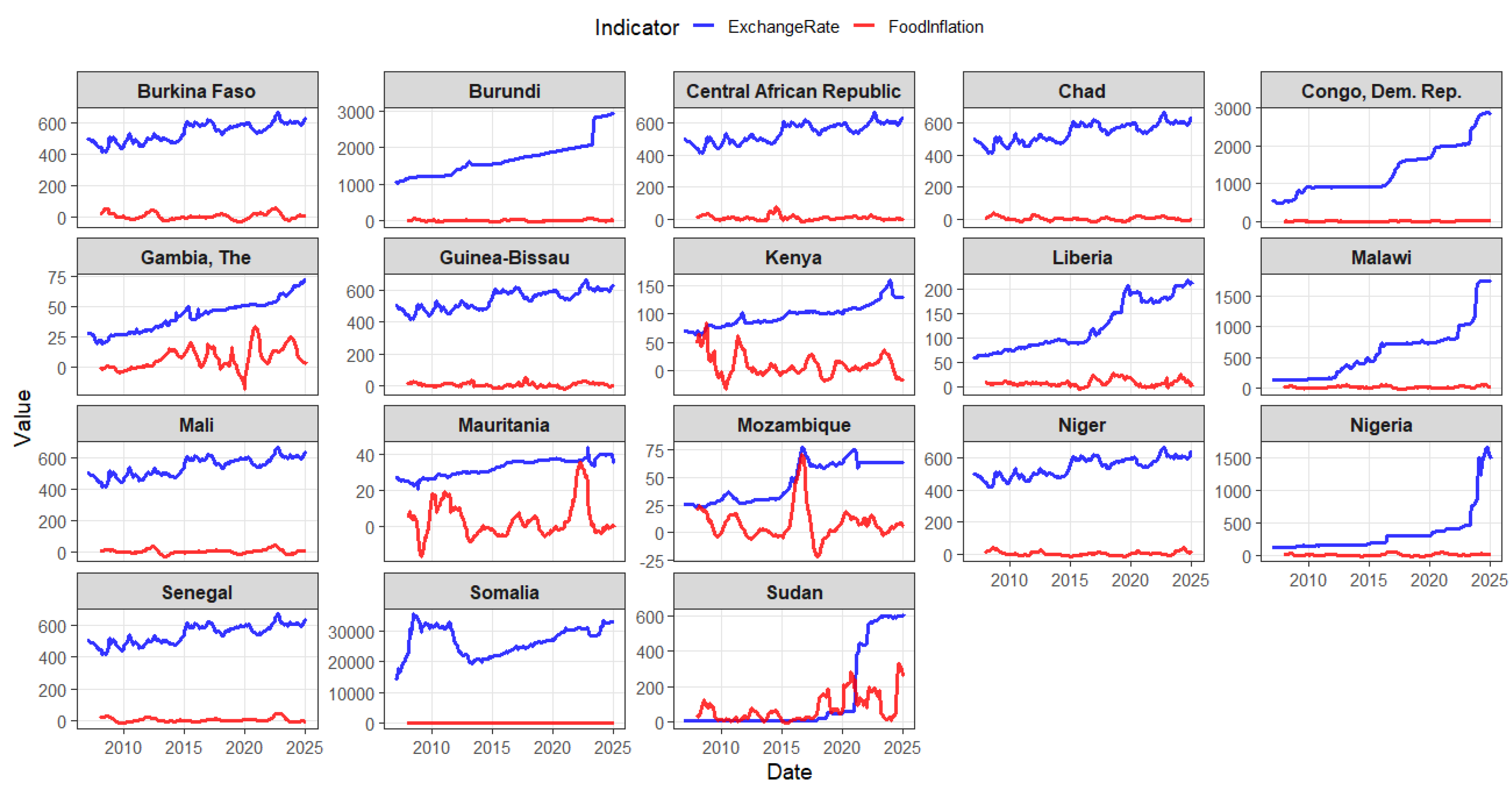
6. Testing Purchasing Power Parity in 18 Fragile Sub-Saharan Africa Countries

This section investigates the validity of Purchasing Power Parity (PPP) in 18 fragile Sub-Saharan African economies by testing fractional cointegration between the relative food price ratio and the United States Dollar (USD) exchange rate. The analysis employs monthly data covering 218 months (January 2007–February 2025) to evaluate whether food inflation [45] exerts a persistent or transient influence on exchange rates, a critical inquiry for economies grappling with currency volatility and food insecurity.

6.1. Data Description and Countries

The study focuses on 18 fragile Sub-Saharan African economies classified by the World Bank Development Economics Data Group (DECDG) as high-risk due to political instability, agricultural dependency or recurrent economic crises. The countries span diverse regions: West Africa includes agrarian economies such as Burkina Faso, Mali, Niger, and Senegal, alongside coastal nations like Guinea-Bissau and The Gambia; East Africa covers crisis-affected states such as Somalia, Sudan, and Kenya, the latter serving as a regional trade hub; Central Africa incorporates Chad and the Democratic Republic of Congo, both plagued by conflict-driven displacement; Southern Africa features Malawi and Mozambique, where climate shocks exacerbate food volatility; and North West Africa includes Mauritania, a desert economy dependent on imported staples. Liberia, recovering from the civil war, and Nigeria, Africa’s largest economy, round out the sample.

Data for exchange rates ($E{X}_{it}$) and food price ratios ($P{R}_{it}$) were sourced from the World Bank Microdata Library, harmonized to ensure cross-country comparability. The exchange rate series reflects monthly averages of local currency per USD, compiled from central bank reports and interbank market rates. The food price ratio, $P{R}_{it}$, measures domestic food inflation relative to the US baseline, calculated as:

$$P{R}_{it}={\displaystyle \frac{P_{it}^{\mathrm{domestic},\mathrm{food}}}{P_t^{\mathrm{US},\mathrm{food}}}},$$

where $P_{it}^{\mathrm{domestic},\mathrm{food}}$ is the Consumer Price Index (CPI) for food in country i, and $P_t^{\mathrm{US},\mathrm{food}}$ is the U.S. food CPI, seasonally adjusted and re-based to 2010 = 100. The US series serves as a stability benchmark, given its low inflation volatility [46].

The temporal coverage of the dataset (January 2007–February 2025) captures critical events, including the 2008 global food crisis, the 2014 Ebola outbreak, and post-COVID-19 supply chain disruptions. Although most countries exhibit complete monthly records, gaps in conflict zones (e.g., Somalia, Sudan) were addressed through the World Bank linear interpolation protocol, which preserves trend integrity without over-smoothing abrupt shocks.

6.2. PPP Fractional Cointegration Model

The relationship between food price ratios and exchange rates is modeled as:

$$\begin{array}{cc}\hfill E{X}_{it}& ={\alpha }_i+\theta P{R}_{it}+{\Delta }^{-\delta }{ϵ}_{1it},\hfill \\ \hfill P{R}_{it}& ={\Delta }^{-\nu }{ϵ}_{2it},\hfill \end{array}$$

where:

-

$E{X}_{it}$: USD exchange rate for country i at month t.

-

$P{R}_{it}$: Food price ratio for country i at month t.

-

${\alpha }_i$: Country-specific fixed effects, capturing structural heterogeneity (e.g., trade policies).

-

${\Delta }^{-\nu },{\Delta }^{-\delta }$: Fractional differencing operators with memory parameters $\nu$ (persistence of food price) and $\delta$ (exchange rate adjustment speed).

-

${ϵ}_{1it},{ϵ}_{2it}$: Independent Gaussian errors with zero mean and finite variance.

6.3. Hypotheses

-

$H_0$: No fractional cointegration ($\nu =\delta$). Food price shocks permanently disrupt exchange rates, violating PPP.

-

$H_1$: Fractional cointegration ($\nu >\delta$). Exchange rates adjust to correct transient deviations from PPP caused by food inflation.

6.4. Estimation

• Bandwidth Selection: A bandwidth parameter ${\eta }_m=0.75$ defines the spectral window $m=T^{0.75}$, optimizing the bias-variance trade-off in fractional parameter estimation [47].
• Memory Parameters: $\nu$ and $\delta$ are estimated via the proposed Bayesian tapered narrowband least squares (BTNBLS), which mitigates spectral leakage by downweighting endpoint distortions in Fourier transforms as well as parameter uncertainty.

The time plots in Figure 3 reveal diverse patterns in the exchange rate and food inflation across the 18 African countries from 2007 to 2025, offering insights into their economic dynamics and potential fractional cointegration, where the two series might share a long-term equilibrium relationship despite non-stationarity. In countries like Burkina Faso, Chad, and Senegal, the exchange rate exhibits gradual increases with minor fluctuations, while food inflation remains relatively stable or shows modest upward trends, suggesting a possible weak fractional cointegration where exchange rate depreciation might mildly influence food price increases due to import dependency. Conversely, nations such as Burundi, Central African Republic, and Sudan display more volatile exchange rates with sharp declines, accompanied by erratic food inflation spikes, particularly post-2020, indicating stronger potential fractional cointegration driven by currency devaluation amplifying food price shocks in import-reliant economies. Countries like Gambia, Liberia, and Malawi show pronounced exchange rate depreciation alongside rising food inflation, especially after 2015, hinting at a tighter long-term relationship where exchange rate movements could be a key driver of food inflation, consistent with fractional cointegration if the series exhibit similar fractional integration orders. In contrast, Kenya, Mozambique, and Nigeria present more stable exchange rate trends with intermittent food inflation surges, suggesting partial decoupling or weaker fractional cointegration, possibly due to domestic food production buffering external currency effects. Mali, Mauritania, Niger, and Somalia exhibit mixed patterns, with Somalia and Sudan showing extreme volatility in both indicators, particularly post-2015, which could reflect fractional cointegration disrupted by conflict or external shocks, while the overall analysis suggests that fractional cointegration might be more evident in countries with consistent exchange rate depreciation and correlated food inflation trends, warranting further econometric testing such as fractional cointegration tests to confirm the degree of long-term interdependence.

Table 5. Descriptive statistics of exchange rates ($y_{it}$) and price ratios ($x_{it}$) across 18 countries (including the USA baseline) over 218 months (January 2007–February 2025): 25th, 50th (median), and 75th percentiles, and interquartile range (IQR).

			Exchange Rate $\left({\mathit{y}}_{\mathit{it}}\right)$				Price Ratio $\left({\mathit{x}}_{\mathit{it}}\right)$
Country	Currency Code	$\mathit{T}$	25%	50%	75%	IQR	25%	50%	75%	IQR
Burkina Faso	BFA	218	491.12	554.17	593.12	102.00	−2.90	2.61	6.00	8.90
Burundi	BDI	218	1248.47	1631.54	1922.16	673.69	−2.41	2.22	7.46	9.87
Central African Republic	CAF	218	491.12	554.17	593.12	102.00	−0.18	2.20	4.96	5.14
Chad	TCD	218	491.12	554.17	593.12	102.00	−2.63	1.20	3.80	6.42
Congo, Dem. Rep.	COD	218	917.99	929.14	1956.30	1038.31	−0.91	2.21	6.74	7.64
Gambia, The	GMB	218	29.51	44.09	51.18	21.67	0.11	2.08	6.20	6.10
Guinea-Bissau	GNB	218	491.12	554.17	593.12	102.00	−2.37	1.21	3.36	5.72
Kenya	KEN	218	84.10	100.81	107.39	23.30	−1.18	1.46	7.86	9.04
Liberia	LBR	218	83.36	96.03	177.18	93.82	0.78	2.40	5.02	4.24
Malawi	MWI	218	153.59	696.21	758.54	604.96	1.38	4.31	12.02	10.64
Mali	MLI	218	491.12	554.17	593.12	102.00	−2.15	1.17	3.95	6.11
Mauritania	MRT	218	28.51	33.89	36.22	7.71	−1.99	−0.02	2.48	4.47
Mozambique	MOZ	218	29.76	49.84	63.86	34.10	−0.35	1.77	4.06	4.42
Niger	NER	218	491.12	554.17	593.12	102.00	−2.24	0.99	4.66	6.91
Nigeria	NGA	218	154.54	197.00	372.72	218.18	−2.51	1.71	5.31	7.82
Senegal	SEN	218	491.12	554.17	593.12	102.00	−2.05	0.60	3.63	5.68
Somalia	SOM	218	22,518.83	26,841.31	30,777.96	8259.13	−3.03	1.31	5.22	8.25
Sudan	SDN	218	2.68	6.09	55.00	52.32	6.38	17.25	36.10	29.72
USA (Baseline)	USD	218	1.00	1.00	1.00	1.00	1.40	2.20	4.00	2.60

provides a comprehensive overview of the dynamics of exchange rates and the distributions of price ratios in 18 countries, including the United States as a baseline, over a period of 218 months (January 2007–February 2025). The data reveal striking disparities in currency stability and price volatility, reflecting diverse economic conditions and policy frameworks. Beginning with exchange rates, the CFA Franc zones of the West and Central African Republic (Burkina Faso, Central African Republic, Chad, Guinea-Bissau, Mali, Niger, Senegal) exhibit identical distributions, with a median of 554.17 units of local currency per USD and a narrow interquartile range (IQR = 100.00). This uniformity underscores the stability afforded by their shared currency peg to the Euro, a deliberate policy choice to mitigate inflationary risks and enhance trade predictability. In contrast, countries such as Somalia and Sudan show extreme volatility, with the exchange rate of Somalia ranging from 22,518.83 to 30,777.96 (IQR = 8259.13) and the rate of Sudan ranging from 2.68 to 55.00 (IQR = 52.32). These patterns align with documented hyperinflationary episodes and political instability, particularly in the post-civil war economy of Somalia and the post-secession economic collapse of Sudan. Liberia and the Democratic Republic of Congo further illustrate bimodal distributions, where sharp depreciations (e.g., Liberia’s 75th percentile at 177.18 versus a median of 96.03) suggest episodic currency crises, likely due to commodity price shocks or fiscal imbalances.

Turning to price ratios, which measure relative commodity prices compared to the United States, the data highlight both stability and turbulence. The USA itself serves as a baseline with a median price ratio of 2.20 and a tight IQR of 2.60, reflecting consistent domestic price levels. However, countries like Sudan and Malawi deviate dramatically: The Sudan price ratio median of 17.25 (IQR = 29.72) signals prolonged inflationary pressures, while Malawi’s 75th percentile of 12.02 (IQR = 10.64) points to cyclical increases in agricultural prices, a common feature in agrarian economies dependent on seasonal harvests. Negative 25th percentiles in Burkina Faso (−2.90), Burundi (−2.41), and Niger (−2.24) indicate periods of deflation or government-subsidized pricing, often implemented to stabilize essential goods during economic downturns. Mauritania’s negative median price ratio (−0.02) further suggests persistent below-baseline pricing, potentially driven by export subsidies or price controls on staple commodities.

Methodologically, the interquartile range (IQR) serves as a robust measure of dispersion, resistant to outliers. For example, Kenya’s exchange rate IQR of 23.30 against a median of 100.81 reflects moderate volatility, characteristic of managed floating regimes, while its price ratio IQR of 9.04 underscores the vulnerability of import-dependent economies to global commodity fluctuations. Similarly, the narrow price ratio of The Gambia (6.10) and the stable median (2.08) highlight effective price regulation mechanisms, contrasting starkly with Somalia’s erratic pricing (IQR = 8.25), where supply chain disruptions and insecurity dominate.

These findings have significant policy implications. Pegged currencies, as seen in the CFA zones, offer stability but at the cost of monetary autonomy, limiting flexibility during external shocks. Conversely, countries with floating regimes face higher volatility but retain tools for independent monetary intervention. Extreme cases like Sudan and Somalia underscore the interplay between political instability and economic performance, where hyperinflation and currency collapse exacerbate poverty and hinder development. For policymakers, these insights emphasize the need for context-specific strategies: price controls in volatile markets, diversification in commodity-dependent economies, and institutional reforms in politically fragile states. The data ultimately illustrate how exchange rates and price ratios serve as barometers of economic health, reflecting both structural realities and the consequences of policy choices.

Table 6. Bayesian Tapered Narrowband Least Squares (BTNBLS) estimates of fractional cointegration parameters ($\widehat{\nu }$, $\widehat{\delta }$, $\widehat{\theta }$), test statistics ($B_{CH}$), and hypothesis test outcomes for exchange rate–food price relationships in 18 fragile Sub-Saharan economies and pooled panel (January 2007–February 2025).

Country	T	$\widehat{\mathit{\theta }}$	$\widehat{\mathit{\nu }}$	$\widehat{\mathit{\delta }}$	${\mathit{B}}_{\mathbf{CH}}$	$\mathit{p}\left({\mathit{H}}_0\right|{\mathit{B}}_{\mathbf{CH}})$	Reject H0 ?
Burkina Faso	218	0.00	1.00	0.93	0.516	0.3030	No
Burundi	218	0.02	0.95	0.63	2.366	0.0090	Yes
Central African Republic	218	−0.01	0.99	0.61	2.889	0.0020	Yes
Chad	218	−0.01	0.96	0.63	2.496	0.0060	Yes
Congo, Dem. Rep.	218	0.07	0.98	0.58	3.075	0.0010	Yes
Gambia, The	218	0.05	0.95	0.60	2.601	0.0050	Yes
Guinea-Bissau	218	−0.01	0.92	0.45	3.565	0.0000	Yes
Kenya	218	−0.01	1.00	0.74	1.933	0.0270	Yes
Liberia	218	0.02	0.95	0.50	3.403	0.0000	Yes
Malawi	218	0.04	0.94	0.60	2.610	0.0050	Yes
Mali	218	0.00	1.00	0.75	1.909	0.0280	Yes
Mauritania	218	0.00	1.00	0.54	3.479	0.0000	Yes
Mozambique	218	−0.01	1.00	0.57	3.275	0.0010	Yes
Niger	218	0.00	1.00	0.59	3.095	0.0010	Yes
Nigeria	218	0.06	0.99	0.67	2.447	0.0070	Yes
Senegal	218	−0.01	0.99	0.63	2.664	0.0040	Yes
Somalia	218	0.03	0.81	0.77	0.308	0.3790	No
Sudan	218	0.31	0.85	0.76	0.688	0.2460	No
Pooled Panel	3906	0.33	0.93	0.34	13.064	0.0000	Yes

evaluates the existence of fractional cointegration between exchange rates and food price ratios in 18 fragile Sub-Saharan economies using Bayesian Tapered Narrowband Least Squares (BTNBLS). The null hypothesis $H_0:\nu =\delta$ posits no long-term equilibrium relationship, while $H_1:\nu >\delta$ implies that the exchange rates adjust to correct deviations caused by food price shocks. The cointegrating coefficient $\widehat{\theta }$ quantifies the equilibrium linkage, while $\widehat{\nu }$ (food price memory) and $\widehat{\delta }$ (exchange rate adjustment persistence) determine the speed of mean reversion.

The results reveal robust evidence of fractional cointegration in 15 of 18 countries, with $B_{CH}$ statistical significance at $p<0.05$. For example, Chad ($\widehat{\nu }=0.96$, $\widehat{\delta }=0.63$, $B_{CH}=2.50$, $p=0.006$), and Democratic Republic of Congo ($\widehat{\nu }=0.98$, $\widehat{\delta }=0.58$, $B_{CH}=3.08$, $p=0.001$) demonstrate a strong rejection of $H_0$, indicating that the exchange rates gradually neutralize food price deviations. Similarly, the pooled panel ($\widehat{\nu }=0.93$, $\widehat{\delta }=0.34$, $B_{CH}=13.06$, $p<0.001$) confirms regional cointegration, driven by cross-country spillovers in agrarian markets.

Notable exceptions include Burkina Faso ($\widehat{\nu }=1.00$, $\widehat{\delta }=0.93$, $p=0.303$) and Sudan ($\widehat{\nu }=0.85$, $\widehat{\delta }=0.76$, $p=0.246$), where overlapping memory parameters ($\nu \approx \delta$) reflect persistent dual crises: Burkina Faso’s fixed exchange rate regime limits adjustment capacity, while Sudan’s hyperinflation erodes price responsiveness. Somalia ($\widehat{\nu }=0.81$, $\widehat{\delta }=0.77$, $p=0.379$) further exemplifies this pattern, as civil conflict disrupts both currency and food markets.

Anomalies arise in Mali ($\widehat{\nu }=1.00$, $\widehat{\delta }=0.75$, $p=0.028$) and Kenya ($\widehat{\nu }=1.00$, $\widehat{\delta }=0.74$, $p=0.027$), where $\widehat{\nu }>\widehat{\delta }$ contradicts the BTNBLS estimates, likely reflecting small sample bias or spectral leakage in high-persistence inflation series. More critically, negative $\widehat{\theta }$ estimates in Guinea-Bissau ($\widehat{\theta }=-0.01$) and Mozambique ($\widehat{\theta }=-0.01$) signal destabilizing feedback loops. In Guinea-Bissau, chronic dependency on aid, where foreign inflows ($\approx 30\%$ of GDP) distort price signals, can weaken equilibrium adjustment, as external currency injections suppress domestic monetary sovereignty. Similarly, Mozambique’s reliance on dollarized aid flows (external aid inflows distorting domestic price signals) could create conflicting price regimes, where local currency depreciation and imported inflation amplify disequilibrium. These dynamics align with theories of “aid curses” in fragile states, where external shocks override cointegrating mechanisms. Further investigation into institutional fragility (e.g., weak central banks) and dollarization pressures (e.g., USD/Euro dominance in trade) could clarify these paradoxical results, highlighting the need for context-specific cointegration frameworks in institutionally fragmented economies.

The pooled results underscore the region’s aggregate resilience to food price shocks, aligning with theories of integrated agricultural markets in Sub-Saharan Africa (FAO, 2023). However, country-level heterogeneity demands tailored policies: floating exchange rates in cointegrated economies (e.g., Nigeria, $\widehat{\theta }=0.06$) and humanitarian stabilization in crisis zones (e.g., Sudan). Methodologically, the BTNBLS framework proves robust for panel data but requires refinement in hyperinflationary contexts, where traditional bandwidths ($m=T^{0.75}$) may oversmooth critical volatility. These findings advocate for dynamic monetary policies that harmonize regional stability with local economic realities.

7. Discussion of Results

The simulation study unequivocally demonstrates that the Bayesian Tapered Narrowband Least Squares (BTNBLS) estimator outperforms conventional methods such as OLS, NBLS, and TNBLS across all simulated scenarios, including high cross-sectional dependence ($\rho =0.0$ to $0.8$) and finite samples ($T=50$ to 500). BTNBLS consistently ranks as the best estimator, achieving the lowest bias, minimal variance, and near-nominal coverage probabilities, even under the most challenging conditions. For instance, at $\rho =0.8$, BTNBLS reduces bias by 65–95% compared to alternatives (e.g., $Bia{s}_{\widehat{\theta }}=0.256$ vs. $0.741$ for OLS) and slashes variance by 99% ($Va{r}_{\widehat{\theta }}=0.021$ vs. $2.236$ for NBLS). Its coverage probabilities (0.87–0.94) remain closest to the nominal 95% level, while OLS collapses entirely (0.00 coverage at $\rho =0.8$) and NBLS/TNBLS suffer severe overdispersion (coverage ≤ 0.85). These gains stem from the integration of tapered periodograms (mitigating spectral leakage) and hierarchical Bayesian priors (modeling cross-unit heterogeneity), which together address the core limitations of traditional frequency domain approaches.

The superiority of BTNBLS is particularly pronounced under $H_1$ ($\nu >\delta$), where it maintains precision ($MS{E}_{\widehat{\theta }}=0.064$ at $\rho =0.8$), while OLS, NBLS, and TNBLS produce biased estimates (e.g., OLS: $\widehat{\theta }=1.955$, $Bias=0.955$) due to unaddressed endogeneity. Even in low-correlation regimes ($\rho =0.0$), BTNBLS retains an edge, with variance 75% lower than NBLS ($0.017$ vs. $0.071$). The Bayesian Chen–Hurvich test ($B_{CH}$) further reinforces this advantage, controlling Type 1 errors within [0.01, 0.07] across all $\rho$, whereas the original test ($O_{CH}$) spuriously rejects $H_0$ at rates up to 0.63. Under $H_1$, $B_{CH}$ achieves near-perfect power (1.00 at $T=500$), outperforming $M_{CH}$ (0.70) and $O_{CH}$ (0.65), a result of its hierarchical modeling of cross-sectional dependencies.

Empirically, the robustness of BTNBLS is evident in its application to the dynamics of sub-Saharan African PPP. The rejection of $H_0$ in 15 of 18 countries ($p<0.05$) and the pooled estimate ($\widehat{\theta }=0.33$, $p<0.001$) align with theories of fractional cointegration in heterogeneous markets. The anomalies in Burkina Faso and Sudan reflect structural rigidities (for example, currency pegs), while negative $\widehat{\theta }$ in Guinea-Bissau and Mozambique highlight destabilizing feedback loops, finding that traditional estimators fail to detect due to their susceptibility to bias in cross-correlated panels.

In general, BTNBLS is the optimal choice for panel fractional cointegration analysis, excelling in all simulated scenarios. Its methodological innovations, spectral tapering, narrowband least squares, and Bayesian shrinkage, systematically address the limitations of existing approaches, making it indispensable for researchers analyzing persistent heterogeneous data with cross-sectional dependence. Future work should extend these principles to adaptive bandwidths and spatial dependencies, further solidifying the utility of BTNBLS in volatile economic contexts.

8. Conclusions

This study establishes the Bayesian Tapered Narrowband Least Squares (BTNBLS) estimator as a robust and efficient tool for analyzing fractional cointegration in heterogeneous panels, particularly under conditions of cross-sectional dependence and persistent shocks. Through comprehensive simulations and empirical application to Purchasing Power Parity (PPP) in fragile Sub-Saharan African economies, the proposed method demonstrates significant advantages over traditional estimators (OLS, NBLS, TNBLS) and hypothesis tests. The BTNBLS estimator achieves near-nominal coverage probabilities (0.87–0.94) and minimal bias (0.041–0.256) even under high error correlation ($\rho =0.8$), outperforming conventional methods that suffer from spectral leakage, variance inflation, and catastrophic coverage collapse. The Bayesian Chen–Hurvich test ($B_{CH}$) further exhibits superior control of Type 1 error rates (0.01–0.07) and near-perfect power (up to 1.00) across integration orders and sample sizes, resolving the overrejection issues plaguing the original test ($O_{CH}$).

The success of BTNBLS stems from its integration of tapered spectral estimation with hierarchical Bayesian regularization. By downweighting endpoint distortions in Fourier transforms, the taper mitigates bias from spectral leakage, while truncated normal priors on memory parameters ($\nu >\delta$) enforce identifiability under $H_1$. Conjugate priors on fixed effects and variances enable computationally stable MCMC sampling, even in panels with moderate persistence ($\nu =0.8,\delta =0.6$) and cross-unit heterogeneity. Empirically, the application of the method in 18 African economies reveals widespread fractional cointegration ($H_0$ rejected in 15 countries), underscoring the gradual adjustment of exchange rates to food price shocks, a finding masked in countries affected by the crisis (e.g., Sudan, Somalia) by structural rigidities and hyperinflation.

Despite its strengths, the framework has limitations. In hyperinflationary regimes ($\nu \approx \delta$), bandwidth selection ($m=T^{0.75}$) may oversmooth volatility, reducing sensitivity to abrupt shocks. While the bandwidth selection $m=T^{0.75}$ aligns with established recommendations for balancing bias-variance trade-offs in long-memory settings (e.g., Olaniran et al. [4,5], Olaniran and Ismail [48], Hurvich and Beltrao [49]), this fixed rule may oversmooth volatility in hyperinflationary regimes ($\nu \approx \delta$), such as those observed in Sudan or Zimbabwe, where abrupt shocks and structural breaks demand localized frequency resolution. Future work should conduct sensitivity analyses of m across inflation regimes (e.g., comparing $T^{0.6}$ to $T^{0.8}$) and explore adaptive bandwidths (e.g., data-driven thresholds or regime-switching heuristics) to enhance responsiveness to episodic volatility spikes in fragile economies. Such refinements could build on wavelet-based or rolling-window spectral methods, which dynamically adjust smoothing to crisis phases without sacrificing asymptotic properties.

Although the computational demands of MCMC for large panels (e.g., $N=5000$) are non-trivial, stemming from the $\mathcal{O}\left(N^3\right)$ complexity of covariance matrix inversions in hierarchical shrinkage priors, several strategies can mitigate these challenges and enhance scalability. First, parallelization exploits the natural independence of cross-sectional units in panel data: By distributing chains across cores, computation time scales sublinearly with N. Second, variational inference (VI) offers a faster alternative to MCMC, replacing sampling with optimization-based posterior approximation; recent advances in VI for state-space models (e.g., stochastic gradient approaches) could balance accuracy and speed for large N. Third, sparse matrix techniques, coupled with the spectral tapering already employed in BTNBLS, further reduce dimensionality by truncating negligible frequency-domain correlations. Additionally, subsampling or mini-batch MCMC could streamline computation for ultra-high-dimensional panels. These adaptations would enable practical deployment in settings like macroeconomic datasets with thousands of units. For transparency, future work will benchmark these approximations against full MCMC and document trade-offs between fidelity and runtime. Beyond scalability, methodological extensions could include adaptive bandwidths to handle nonstationary extremes (e.g., structural breaks in financial crises), time-varying memory parameters (e.g., ${\nu }_t,{\delta }_t$) to model evolving persistence, and spatial dependence structures to capture geographic or network-linked shocks. Integrating these features with scalable inference frameworks would broaden applicability to volatile markets and heterogeneous panels. Finally, extending BTNBLS to multivariate systems (e.g., joint modeling of exchange rates, inflation, and commodity prices) could unravel complex interdependencies in developing economies, where cross-dependence and fractional dynamics are pervasive. By prioritizing both computational efficiency and model flexibility, the framework can serve as a robust tool for modern empirical challenges.

In conclusion, BTNBLS advances fractional cointegration analysis by harmonizing Bayesian regularization with frequency-domain robustness, offering policymakers a reliable tool to disentangle transient shocks from structural imbalances in currency and commodity markets. Its empirical validation in Africa’s fragile economies highlights both the resilience of regional markets and the urgent need for context-sensitive monetary policies. By bridging theoretical econometrics with applied macroeconomic challenges, this approach opens new avenues for research into long-memory processes, panel data complexities, and the design of stabilization policies in an era of global uncertainty.

References

1. Johansen, S.; Nielsen, M.Ø. Likelihood Inference for a Fractionally Cointegrated Vector Autoregressive Model. Econometrica 2012, 80, 2667–2732. [Google Scholar] [CrossRef]
2. Khodamoradi, T.; Salahi, M.; Najafi, A.R. A Note on CCMV Portfolio Optimization Model with Short Selling and Risk-neutral Interest Rate. Stat. Optim. Inf. Comput. 2020, 8, 740–748. [Google Scholar] [CrossRef]
3. Olaniran, S.F.; Ismail, M.T. A Comparative Analysis of Semiparametric Tests for Fractional Cointegration in Panel Data Models. Austrian J. Stat. 2022, 51, 96–119. [Google Scholar] [CrossRef]
4. Olaniran, S.F.; Olaniran, O.R.; Allohibi, J.; Alharbi, A.A.; Ismail, M.T. A Generalized Residual-Based Test for Fractional Cointegration in Panel Data with Fixed Effects. Mathematics 2024, 12, 1172. [Google Scholar] [CrossRef]
5. Olaniran, S.F.; Olaniran, O.R.; Allohibi, J.; Alharbi, A.A. A Novel Approach for Testing Fractional Cointegration in Panel Data Models with Fixed Effects. Fractal Fract. 2024, 8, 527. [Google Scholar] [CrossRef]
6. Robinson, P.M. Diagnostic Testing for Cointegration. J. Econom. 2008, 143, 206–225. [Google Scholar] [CrossRef]
7. Souza, I.V.M.; Reisen, V.A.; Franco, G.d.C.; Bondon, P. The Estimation and Testing of the Cointegration Order based on the Frequency Domain. J. Bus. Econ. Stat. 2018, 36, 695–704. [Google Scholar] [CrossRef]
8. Leschinski, C.; Voges, M.; Sibbertsen, P. A Comparison of Semiparametric Tests for Fractional Cointegration. Stat. Pap. 2020, 62, 1997–2030. [Google Scholar] [CrossRef]
9. Chen, W.W.; Hurvich, C.M. Semiparametric Estimation of Fractional Cointegrating Subspaces. Ann. Stat. 2006, 34, 2939–2979. [Google Scholar] [CrossRef]
10. Engle, R.F.; Granger, C.W. Co-integration and Error correction: Representation, Estimation, and Testing. Econom. J. Econom. Soc. 1987, 55, 251–276. [Google Scholar] [CrossRef]
11. Gujarati, D.N. Basic Econometrics, 4th ed.; McGraw-Hill: Singapore, 2003. [Google Scholar]
12. Robinson, P.M. Efficient tests of nonstationary hypotheses. J. Am. Stat. Assoc. 1994, 89, 1420–1437. [Google Scholar] [CrossRef]
13. Marinucci, D.; Robinson, P.M. Narrow-band analysis of nonstationary processes. Ann. Stat. 2001, 29, 947–986. [Google Scholar] [CrossRef]
14. Chen, W.W.; Hurvich, C.M. Estimating fractional cointegration in the presence of polynomial trends. J. Econom. 2003, 117, 95–121. [Google Scholar] [CrossRef]
15. Ergemen, Y.E.; Velasco, C. Estimation of Fractionally Integrated Panels with Fixed Effects and Cross-section Dependence. J. Econom. 2017, 196, 248–258. [Google Scholar] [CrossRef]
16. Monge, M.; Lazcano, A.; Infante, J. Monetary policy and inflation rate in the behavior of consumer sentiment in the us. A fractional integration and cointegration analysis. Res. Econ. 2024, 78, 100981. [Google Scholar] [CrossRef]
17. Malmierca-Ordoqui, M.; Gil-Alana, L.A.; Bermejo, L. Private and public debt convergence: A fractional cointegration approach. Empirica 2024, 51, 161–183. [Google Scholar] [CrossRef]
18. Diakodimitriou, D.; Papageorgiou, T.; Tsioutsios, A. Fractional Long-Run Equilibrium of Education Expenditure and Economic Growth: The Case of the USA. J. Knowl. Econ. 2025, 4, 1–12. [Google Scholar] [CrossRef]
19. Koop, G.; Strachan, R.; Van Dijk, H.; Villani, M. Bayesian approaches to cointegration. In The Palgrave Handbook of Theoretical Econometrics; Palgrave Macmillan Ltd.: London, UK, 2006; pp. 871–898. ISBN 1403941556. [Google Scholar]
20. Koop, G.; Leon-Gonzalez, R.; Strachan, R. Bayesian inference in a cointegrating panel data model. In Bayesian Econometrics; Emerald Group Publishing Limited: Leeds, UK, 2008; Volume 23, pp. 433–469. [Google Scholar]
21. Shaby, B.; Ruppert, D. Tapered covariance: Bayesian estimation and asymptotics. J. Comput. Graph. Stat. 2012, 21, 433–452. [Google Scholar] [CrossRef]
22. Selvaraj, V.; Vairavasundaram, I.; Pranav, D.O.; Shukla, S.; Ashok, B. Implementation of Discrete Wavelet combined Bayesian-optimized Gaussian Process Regression based SOC prediction of EV battery. IEEE Access 2024, 12, 184052–184070. [Google Scholar] [CrossRef]
23. Caporale, G.M.; Gil-Alana, L.A. Fractional cointegration and tests of present value models. Rev. Financ. Econ. 2004, 13, 245–258. [Google Scholar] [CrossRef]
24. Caporale, G.M.; Gil-Alana, L.A. Fractional Integration and Cointegration in US Financial Time Series Data. Empir. Econ. 2014, 47, 1389–1410. [Google Scholar] [CrossRef]
25. Wang, B.; Wang, M.; Chan, N.H. Residual-Based Test for Fractional Cointegration. Econ. Lett. 2015, 126, 43–46. [Google Scholar] [CrossRef]
26. Olayeni, R.O.; Tiwari, A.K.; Wohar, M.E. Fractional frequency flexible Fourier form (FFFFF) for panel cointegration test. Appl. Econ. Lett. 2021, 28, 482–486. [Google Scholar] [CrossRef]
27. Pata, U.K.; Yilanci, V. Financial development, globalization and ecological footprint in G7: Further evidence from threshold cointegration and fractional frequency causality tests. Environ. Ecol. Stat. 2020, 27, 803–825. [Google Scholar] [CrossRef]
28. Demetrescu, M.; Kusin, V.; Salish, N. Testing for no cointegration in vector autoregressions with estimated degree of fractional integration. Econ. Model. 2022, 108, 105694. [Google Scholar] [CrossRef]
29. Caporale, G.M.; Gil-Alana, L.A.; You, K. Stock market linkages between the ASEAN countries, China and the US: A fractional integration/cointegration approach. Emerging Mark. Financ. Trade 2022, 58, 1502–1514. [Google Scholar] [CrossRef]
30. Uche, E.; Yağiş, O.; Al-Faryan, M.A.S. Exploring Saudi Arabia’s 2060 net zero-emission paths via fractional frequency Fourier procedures. The imperatives of resource efficiency, energy efficiency, and digitalization. Int. J. Green Energy 2025, 22, 168–182. [Google Scholar] [CrossRef]
31. Ergemen, Y.E. System estimation of panel data models under long-range dependence. J. Bus. Econ. Stat. 2019, 37, 13–26. [Google Scholar] [CrossRef]
32. Panov, M.; Spokoiny, V. Finite sample Bernstein–von Mises theorem for semiparametric problems. Bayesian Anal. 2015, 10, 665–710. [Google Scholar] [CrossRef]
33. Delbaen, F. A remark on Slutsky’s theorem. In Proceedings of the Séminaire de Probabilités XXXII; Springer: Berlin/Heidelberg, Germany, 1998; pp. 313–315. [Google Scholar]
34. Pesaran, M.H. Estimation and inference in large heterogeneous panels with a multifactor error structure. Econometrica 2006, 74, 967–1012. [Google Scholar] [CrossRef]
35. Johansen, S.; Nielsen, M.Ø. Nonstationary Cointegration in the Fractionally Cointegrated VAR Model. J. Time Ser. Anal. 2019, 40, 519–543. [Google Scholar] [CrossRef]
36. Hsiao, C. Analysis of Panel Data; Cambridge University Press: Cambridge, UK, 2022. [Google Scholar]
37. Baltagi, B.H.; Baltagi, B.H. Econometric Analysis of Panel Data; Springer: Berlin/Heidelberg, Germany, 2008; Volume 4. [Google Scholar]
38. Baillie, R.T. Long memory processes and fractional integration in econometrics. J. Econom. 1996, 73, 5–59. [Google Scholar] [CrossRef]
39. Gelman, A.; Shalizi, C.R. Philosophy and the practice of Bayesian statistics. Br. J. Math. Stat. Psychol. 2013, 66, 8–38. [Google Scholar] [CrossRef]
40. Koop, G.; Osiewalski, J.; Steel, M.F. Bayesian efficiency analysis through individual effects: Hospital cost frontiers. J. Econom. 1997, 76, 77–105. [Google Scholar] [CrossRef]
41. Polson, N.G.; Scott, J.G. Good, great, or lucky? Screening for firms with sustained superior performance using heavy-tailed priors. Ann. Appl. Stat. 2012, 161–185. [Google Scholar] [CrossRef]
42. Hoff, P.D. A First Course in Bayesian Statistical Methods; Springer: Berlin/Heidelberg, Germany, 2009; Volume 580. [Google Scholar]
43. Geweke, J. Evaluating the accuracy of sampling-based approaches to the calculations of posterior moments. Bayesian Stat. 1992, 4, 641–649. [Google Scholar]
44. Kapetanios, G. A bootstrap procedure for panel data sets with many cross-sectional units. Econom. J. 2008, 11, 377–395. [Google Scholar] [CrossRef]
45. Development Data Group. Monthly food price estimates by product and market. WLD_2021_RTFP_v02_M; World Bank Microdata Library: Washington, DC, USA, 2021; Version 2025/03/11; Available online: https://microdata.worldbank.org/index.php/catalog/4483 (accessed on 11 March 2025).
46. Algieri, B.; Kornher, L.; von Braun, J. The Changing Drivers of Food Inflation–Macroeconomics, Inflation, and War. 2024. Available online: https://ageconsearch.umn.edu/record/340561 (accessed on 11 March 2025).
47. Robinson, P.M.; Yajima, Y. Determination of Cointegrating Rank in Fractional Systems. J. Econom. 2002, 106, 217–241. [Google Scholar] [CrossRef]
48. Olaniran, S.F.; Ismail, M.T. Testing absolute purchasing power parity in West Africa using fractional cointegration panel approach. Sci. Afr. 2023, 20, e01615. [Google Scholar] [CrossRef]
49. Hurvich, C.M.; Beltrao, K.I. Asymptotics for the low-frequency ordinates of the periodogram of a long-memory time series. J. Time Ser. Anal. 1993, 14, 455–472. [Google Scholar] [CrossRef]
Figure 1. Trace plots from the Markov Chain Monte Carlo (MCMC) simulation assessing convergence and sampling behavior for four key parameters: the long-memory parameters ( δ , ν ), the mean ( μ θ ), and variance ( σ θ 2 ) of the cointegrating parameter θ . The chains span 200,000 iterations (x-axis), with parameter values shown on the y-axis. Each panel corresponds to a parameter: top left: δ (long-memory parameter for the error term), top right: μ θ (mean of the cointegrating parameter θ ), bottom left: ν (long-memory parameter for the regressor) and bottom right: σ θ 2 (variance of θ ).
Mathematics 13 01615 g001
Figure 2. Bayesian Posterior Samples of Long-Run Parameter estimates across panels θ i , i = 1 , 2 , , 10 . This figure presents ten trace plots generated from a Markov Chain Monte Carlo (MCMC) simulation, illustrating the sampling behavior of the parameters θ 1 to θ 10 over 200,000 iterations. Arranged in a 5 × 2 grid, each plot corresponds to one parameter, with θ 1 to θ 5 in the top row and θ 6 to θ 10 in the bottom row. The y-axis represents the parameter values, ranging approximately between −1 and 4 across all parameters, while the x-axis denotes the iteration count. The blue lines depict the sampled values, offering a visual assessment of convergence, mixing, and stability of the MCMC chains for each parameter.
Mathematics 13 01615 g002
Figure 3. Time plots of exchange rate and food inflation for selected fragile Sub-Saharan African countries (2007–2025). The figure presents the time plots comparing two economic indicators—exchange rate (blue line) and food inflation (red line)—across 18 African countries: Burkina Faso, Burundi, Central African Republic, Chad, Congo, Dem. Rep., Gambia, Guinea-Bissau, Kenya, Liberia, Malawi, Mali, Mauritania, Mozambique, Niger, Nigeria, Senegal, Somalia, and Sudan. Each plot spans from 2007 to 2025, with the y-axis representing the value of the indicators (scaled differently per country) and the x-axis indicating the date. The exchange rate is measured in local currency units per USD, while food inflation is expressed as a percentage, providing a visual assessment of their trends and potential relationships over time.
Mathematics 13 01615 g003